2. Stochastic model

The purpose of this Section is to introduce the stochastic model that forms the basis for our analysis.

For $i\in \{1,\ldots, m\}$ and $k\in \{1,\ldots, n\}$ , let $S_{i,k}$ denote the incremental claims of accident year i in the development year k (payments or incurred amounts). We assume that the random variables $S_{i,k}$ are observable up to the calendar year p (i.e., for $i+k\le p+1$ ) for a p with $\max(m,n)\le p \lt m+n-1$ . Let $\mathcal{A}\,:\!=\,\{1,\ldots,m\}\times\{1,\ldots,n\}$ denote the set of all pairs of accident and development years and let $\mathcal{O}\,:\!=\,\{(i,k)\in\mathcal{A}\,|\, i+k\le p+1\}$ be the subset containing the indices of the observable increments. The goal of a reserving method is to predict the increments $S_{i,k}$ with $(i,k)\in \mathcal{P}\,:\!=\,\mathcal{A}\setminus\mathcal{O}$ . We define

\begin{align*}I(k)\,:\!=\,\min\{p-k+1,m\}\quad\text{and}\quad K(i)\,:\!=\,\min\{p-i+1,n\}, \end{align*}

such that $S_{1,k},\ldots,S_{I(k),k}$ are the observable increments from development year k and $S_{i,1},\ldots,S_{i,K(i)}$ are the observable increments from accident year i.

We assume that ‘correct’ volumes exist, which are not known, and model them as random variables $V_1,\ldots,V_m$ . Similarly to Riegel (Reference Riegel2018), we can w.l.o.g. assume $V_m=v_m$ . Then there are random errors $E_1,\ldots,E_{m-1}$ such that

(2.1) \begin{align} V_i\,:\!=\,(1+E_i+\ldots + E_{m-1})\cdot v_i\end{align}

for $i=1,\ldots, m-1$ . Let $\mathscr{V}\,:\!=\,\sigma(V_1,\ldots,V_m)=\sigma(E_1,\ldots,E_{m-1})$ be the sigma algebra generated by $V_1,\ldots,V_m$ . Our stochastic model is given by the following three assumptions.

Model Assumption 2. There are a parameter $\varepsilon \gt 0$ and known factors $\lambda_1,\ldots,\lambda_{m-1} \gt 0$ such that $E_i$ is normally distributed with

\begin{align*}\mathrm{E}(E_i)=0 \quad\text{and} \quad \mathrm{Var}(E_i)=\lambda_i^2\varepsilon^2\,=\!:\,\varepsilon_i^2. \end{align*}

Model Assumption 3. Conditionally, given $\mathscr{V}$ , the increments $S_{i,k}$ , $(i,k)\in \mathcal{A}$ , are normally distributed. There are parameters $\mu_1,\ldots, \mu_n$ and $\sigma_1,\ldots,\sigma_n \gt 0$ such that

\begin{align*}\mathrm{E}(S_{i,k}|\mathscr{V})=V_i\mu_k \quad\text{and}\quad \mathrm{Var}(S_{i,k}|\mathscr{V})=v_i\sigma_k^2. \end{align*}

Remark 2.2. In Model Assumption 1, we require the errors $E_i$ to be independent. In reality, there is potential for systematic errors in indexation. For instance, loss indexation can be based on an officially published index, which might systematically under- or overestimate the real claims inflation. In our framework, a simple way to account for such a systematic error is to replace the assumption $V_i\,:\!=\,(1+E_i+\ldots + E_{m-1})\cdot v_i$ with the more complex assumption:

\begin{align*} V_i\,:\!=\,(1+E_i+\ldots + E_{m-1}+(m-i)F)\cdot v_i \end{align*}

with an additional random error $F\sim \mathrm{Norm}(0,\varphi^2)$ that is independent of $(E_1,\ldots,E_{m-1})$ . The EM algorithm still works with this extension, but we are reluctant to further increase the complexity of the model.

Remark 2.3. If the errors $E_i$ are small (i.e., $|E_i|\ll 1$ ), then the assumption $V_i=(1+E_i+\ldots + E_{m-1})\cdot v_i$ implies

\begin{align*} \frac{1}{v_i} =\frac{1+E_i+\ldots + E_{m-1}}{V_i}\approx \frac{1}{V_i}\cdot (1+E_i)\cdots (1+E_{m-1}). \end{align*}

The corresponding model assumption in Riegel (Reference Riegel2018) is

\begin{align*} \frac{1}{\widehat{v}_i} = \frac{1}{v_i}\cdot f_i\cdots f_{m-1} \end{align*}

with lognormally distributed factors $f_i$ that satisfy $\mathrm{E}(f_i)=1$ and $\mathrm{Var}(f_i)=\varepsilon_i^2$ . For small coefficients of variation, the $f_i-1$ are approximately normally distributed, which shows the similarity of the two assumptions. Note that the parameters $\varepsilon_i$ have a similar meaning in both models. Comparing the two formulas, we also see the main difference in the approaches. In Riegel (Reference Riegel2018), the ‘correct’ volumes are interpreted as unknown parameters, which are denoted by $v_i$ and the available volumes are modeled as observable random variables $\widehat{v}_i$ . In this paper, the available volumes are interpreted as known parameters $v_i$ and the ‘correct’ volumes are modeled as non-observable random variables $V_i$ .

Remarks 2.3 and 2.4 show that our model is actually an approximation of the generalized additive model in Riegel (Reference Riegel2018). The approximation is quite good for small $\varepsilon_i$ and has the big advantage that parameter estimation can be conducted with the EM algorithm, which is an established statistical approach that leads to simple iteration formulas in our situation. It should be noted that pricing actuaries generally only take volumes into account if they consider the quality to be appropriate. In this situation, there is a good chance that the $\varepsilon_i$ are small.

Remark 2.5. In the limiting case $\varepsilon \to 0$ , we have $V_i=v_i$ , that is, the $S_{i,k}$ are unconditionally independent,

\begin{align*} \mathrm{E}(S_{i,k})=\mathrm{E}(S_{i,k}|\mathscr{V})=v_i\mu_k\qquad \text{and}\qquad \mathrm{Var}(S_{i,k})=\mathrm{Var}(S_{i,k}|\mathscr{V})=v_i\sigma_k^2. \end{align*}

This means that for $\varepsilon\to 0$ , we obtain the classical additive model with the additional assumption that the increments $S_{i,k}$ are normally distributed.

3. Parameter estimation

In this section, we apply the EM algorithm to calculate the maximum likelihood estimators for the unknown parameters. The EM algorithm (see Dempster et al., Reference Dempster, Laird and Rubin1977) provides a generic iteration to find (local) maxima of the log-likelihood when there are so-called latent variables, that is, random variables that are not observable. In our case, we treat the unknown volumes $V_i$ (or equivalently the errors $E_i$ ) as latent variables. We assume $I(n) \gt 1$ to avoid problems with the estimation of $\sigma_n$ . A pragmatic solution for the case $I(n)=1$ is provided in Remark 3.2.

Let $S\,:\!=\,(S_{i,k})_{(i,k)\in \mathcal{O}}$ denote the vector of the observable incremental losses and let $E\,:\!=\,(E_1,\ldots,E_{m-1})$ be the vector containing the estimation errors for the volumes. In the following, we derive the EM iteration for the estimation of $m_k$ , $\sigma_k$ and $\varepsilon$ . As mentioned in Remark 2.1, it often makes sense to use an external estimator $\widehat{\varepsilon}^{\mathrm{ext}}$ instead of the maximum likelihood estimator for $\varepsilon$ . The necessary modification to the iteration is described in Remark 3.3.

Let $\Theta \,:\!=\,(\mu,\sigma,\varepsilon)\,:\!=\,(\mu_1,\ldots, \mu_n, \sigma_1,\ldots, \sigma_n,\varepsilon)$ . The density $p_{(E,S)}(\,\cdot\, ;\,\Theta)$ of (E,S) has a simple form:

\begin{align*}& p_{(E, S)} (e, s;\,\Theta)=p_{(E, S)} ((e_i)_{i=1,\ldots,m-1}, (s_{i,k})_{(i,k)\in \mathcal{O}};\, \Theta) =\\ & \phantom{aaaaaaaaa}=\prod_{i=1}^{m-1}\frac{1}{\sqrt {2\pi\lambda_i^2\varepsilon^2}}\exp\!\left(-\frac{e_i^2}{2\lambda_i^2\varepsilon^2} \right) \\ & \phantom{aaaaaaaaaaaaa} \cdot \prod_{(i,k)\in \mathcal{O}}\frac{1}{\sqrt {2\pi v_i \sigma_k^2}}\exp\!\left(-\frac{(s_{i,k}-(1+e_i+\ldots+e_{m-1})\cdot v_i \mu_k)^2}{2v_i\sigma_k^2} \right).\end{align*}

The log-likelihood of the observable data S is given by:

(3.1) \begin{align} l_S(\Theta)=\log p_S(S;\,\Theta)=\log \int_{\unicode{x211D}^{m-1}}p_{(E,S)}(e, S;\,\Theta)\, de,\end{align}

which is not as simple as the log-likelihood $l_{(E,S)}(\Theta)=\log\!(p_{(E,S)}(E,S;\,\Theta))$ of the complete data (E,S). The EM algorithm is designed to iteratively find (local) maxima of the observable log-likelihood in such situations.

The EM iteration alternates between performing an expectation step (E step), which calculates the expected log-likelihood function using the current estimates for the parameters, and a maximization step (M step), which computes new estimates for the parameters, maximizing the expected log-likelihood found in the E step. These updated parameter estimates are then used to determine the distribution of the latent variables in the next E step. In our case, we define

\begin{align*}Q(\Theta|\Theta^{\prime})\,:\!=\,\mathrm{E}_{E|S;\,\Theta^{\prime}}\big(\log\!(p_{(E,S)}(E,S;\,\Theta))\big)=\mathrm{E}_{E|S;\,\Theta^{\prime}}\big(l_{(E,S)}(\Theta)\big) \end{align*}

and start with an initial parameter vector $\widehat{\Theta}^{(0)}$ . Given $\widehat{\Theta}^{(\nu)}$ , we calculate $Q(\Theta|\widehat{\Theta}^{(\nu)})$ in the E step and in the M step we choose $\widehat{\Theta}^{(\nu+1)}$ to be a value that maximizes $Q(\,\cdot\,|\widehat{\Theta}^{(\nu)})$ .

Proposition 3.1 provides the conditional distribution of the latent variable vector E, given S and $\Theta$ , which is needed in the calculation of the expected log-likelihood in the E step. We define

\begin{align*} G(\Theta)\,:\!=\,\left( \begin{array}{c@{\quad}c@{\quad}c} g_{1,1}(\Theta) & \cdots & g_{1,m-1}(\Theta) \\ \vdots & & \vdots \\ g_{m-1,1}(\Theta) & \cdots & g_{m-1,m-1}(\Theta) \end{array}\right)\quad \text{and}\quad h(\Theta)\,:\!=\,\left(\begin{array}{c} h_1(\Theta) \\ \vdots \\ h_{m-1}(\Theta) \end{array} \right) \end{align*}

by

\begin{align*} g_{i,j}(\Theta)\,:\!=\,\delta_{i,j}\frac{1}{\lambda_i^2\varepsilon^2}+ \sum_{\nu=1}^{\min(i,j)}\sum_{k=1}^{K(\nu)}\frac{v_\nu \mu_k^2}{\sigma_k^2}\quad \text{and}\quad h_i(\Theta)\,:\!=\,\sum_{\nu=1}^{i}\sum_{k=1}^{K(\nu)}\frac{s_{\nu,k} \mu_k-v_{\nu} \mu_k^2}{\sigma_k^2} \end{align*}

for $1\le i,j\le m-1$ , where $\delta_{i,j}$ denotes the Kronecker symbol. According to Lemma E.1 in Riegel (Reference Riegel2015), the matrix $G(\Theta)$ is invertible. Let

\begin{align*} A(\Theta)\,:\!=\,\left( \begin{array}{c@{\quad}c@{\quad}c} a_{1,1}(\Theta) & \cdots & a_{1,m-1}(\Theta) \\ \vdots & & \vdots \\ a_{m-1,1}(\Theta) & \cdots & a_{m-1,m-1}(\Theta) \end{array} \right)\,:\!=\,G(\Theta)^{-1}\quad \end{align*}

and

\begin{align*} b(\Theta)\,:\!=\,\left(\begin{array}{c} b_1(\Theta) \\ \vdots \\ b_{m-1}(\Theta) \end{array} \right)\,:\!=\,A(\Theta)h(\Theta). \end{align*}

Proof. With $e\,:\!=\,(e_1,\ldots,e_{m-1})^t$ , we have

\begin{align*}-\sum_{i=1}^{m-1} \frac{e_i^2}{2\lambda_i^2\varepsilon^2} - \sum_{(i,k)\in \mathcal{O}} & \frac{\left(s_{i,k}-(1+e_i+\ldots+e_{m-1})\cdot v_i \mu_k \right)^2}{2v_i \sigma_k^2}+c_1 \\ & \phantom{aaaa} =-\frac{1}{2} \sum_{i=1}^{m-1}\sum_{j=1}^{m-1}g_{i,j}(\Theta)e_ie_j+\sum_{i=1}^{m-1}h_{i}(\Theta)e_i+c_2 \\& \phantom{aaaa} = -\frac{1}{2} e^tG(\Theta)e+e^th(\Theta) +c_2 \\& \phantom{aaaa} =-\frac{1}{2} e^tA(\Theta)^{-1}e+e^tA(\Theta)^{-1} b(\Theta) +c_2\\ & \phantom{aaaa} = -\frac{1}{2}(e-b(\Theta))^t A(\Theta)^{-1}(e-b(\Theta)) +c_3, \end{align*}

where $c_1$ , $c_2$ , and $c_3$ do not depend on e.

Before we derive the formulas for the EM iteration, we need some additional notation. Let

\begin{align*}\kappa_{i,j}\,:\!=\,\begin{cases} 0 & \text{ for }j \lt i \\ 1 & \text{ for }j\ge i\end{cases} \end{align*}

and

\begin{align*}\kappa_i\,:\!=\,(\kappa_{i,1},\ldots, \kappa_{i,m-1})^t\in \unicode{x211D}^{m-1}. \end{align*}

Then we define for $i=1,\ldots,m$

\begin{align*}d_i(\Theta)\,:\!=\,\mathrm{E}(1+E_i+\ldots+E_{m-1} | S,\Theta)=1+\kappa_i^t b(\Theta) \end{align*}

and for $i,j=1,\ldots,m$

\begin{align*}c_{i,j}(\Theta)\,:\!=\,\mathrm{Cov}(1+E_i+\ldots+E_{m-1}, 1+E_j+\ldots+E_{m-1}| S,\Theta)=\kappa_i^t A(\Theta)\kappa_j. \end{align*}

Note that $\kappa_m=0\in \unicode{x211D}^{m-1}$ , $d_m(\Theta)=1$ and $c_{i,j}\,:\!=\,0$ for $\max(i,j)=m$ .

Given an estimate $\widehat{\Theta}^{(\nu)}$ , we can use Proposition 3.1 to perform the E step:

\begin{align*} Q( & \Theta|\widehat{\Theta}^{(\nu)}) =\mathrm{E}_{E|S;\widehat{\Theta}^{(\nu)}}\Big(l_{(E,S)}(\Theta)\vphantom{\sum_{q=1}^{p}}\Big) \\ & = \mathrm{E}_{E|S;\widehat{\Theta}^{(\nu)}} \left(\sum_{i=1}^{m-1} \left(-\log\!(\varepsilon) - \frac{E_i^2}{2\lambda_i^2\varepsilon^2} \right)\right)\end{align*}

\begin{align*} & \phantom{aa} + \mathrm{E}_{E|S;\widehat{\Theta}^{(\nu)}}\left(\sum_{(i,k)\in\mathcal{O}}\left(-\log\!(\sigma_k)-\frac{(S_{i,k}-(1+E_i+\ldots+E_{m-1})\cdot v_i \mu_k)^2}{2v_i \sigma_k^2 } \right)\right)+c\\ & = \sum_{i=1}^{m-1} \left( -\log\!(\varepsilon) - \frac{a_{i,i}(\widehat{\Theta}^{(\nu)}) + b_i(\widehat{\Theta}^{(\nu)})^2}{2\lambda_i^2\varepsilon^2} \right) \\ & \phantom{aa} + \sum_{(i,k)\in \mathcal{O}}\left(-\log\!(\sigma_k)-\frac{v_i^2 \mu_k^2c_{i,i}(\widehat{\Theta}^{(\nu)}) + (S_{i,k}-d_{i}(\widehat{\Theta}^{(\nu)})v_i\mu_k)^2}{2v_i \sigma_k^2} \right)+c\end{align*}

with a suitable constant c. We have

\begin{align*} \frac{\partial}{\partial \mu_k}Q(\Theta|\widehat{\Theta}^{(\nu)}) & =\sum_{i=1}^{I(k)}\frac{d_{i}(\widehat{\Theta}^{(\nu)})S_{i,k}-(c_{i,i}(\widehat{\Theta}^{(\nu)})+d_{i}(\widehat{\Theta}^{(\nu)})^2) v_i \mu_k}{\sigma_k^2}, \\ \frac{\partial}{\partial \sigma_k}Q(\Theta|\widehat{\Theta}^{(\nu)}) & =\sum_{i=1}^{I(k)}-\frac{1}{\sigma_k}+ \frac{(S_{i,k}-d_{i}(\widehat{\Theta}^{(\nu)})v_i\mu_k)^2 + v_i^2 \mu_k^2 c_{i,i}(\widehat{\Theta}^{(\nu)}) }{v_i\sigma_k^3},\quad \text{and}\\\frac{\partial}{\partial \varepsilon}Q(\Theta|\widehat{\Theta}^{(\nu)}) & =\sum_{i=1}^{m-1}\left(-\frac{1}{\varepsilon}+\frac{a_{i,i}(\widehat{\Theta}^{(\nu)})+b_{i}(\widehat{\Theta}^{(\nu)})^2 }{\lambda_i^2\varepsilon^3}\right).\end{align*}

In the M step, we have to set these partial derivations to zero to calculate $\widehat{\Theta}^{(\nu+1)}$ . Using the notation $\widehat{\Theta}^{(\nu)}\,:\!=\,(\widehat{\mu}_1^{(\nu)},\ldots,\widehat{\mu}_n^{(\nu)}, \widehat{\sigma}^{(\nu)}_1,\ldots, \widehat{\sigma}^{(\nu)}_n,\widehat{\varepsilon}^{(\nu)})$ , we obtain the following iteration.

Iteration for parameter estimation: We select an initial vector $\widehat{\Theta}^{(0)}$ . For instance, we can use the the maximum likelihood estimators in the classical additive model (with the assumption of normal distributions), that is,

\begin{align*}\widehat{\mu}_k^{(0)}\,:\!=\,\widehat{\mu}_k^{\mathrm{MLE}}\,:\!=\,\frac{\sum_{i=1}^{I(k)}S_{i,k}}{\sum_{i=1}^{I(k)} v_i} \quad \text{and} \quad (\widehat{\sigma}^{(0)}_k)^2\,:\!=\,(\widehat{\sigma}^{\mathrm{MLE}}_k)^2\,:\!=\,\frac{1}{I(k)}\sum_{i=1}^{I(k)}v_i\left(\frac{S_{i,k}}{v_i}-\widehat{\mu}_k^{(0)}\right)^2 \end{align*}

and select a reasonable initial value $\widehat{\varepsilon}^{(0)}$ . Given $\widehat{\Theta}^{(\nu)}$ , we calculate $\widehat{\Theta}^{(\nu+1)}$ with

\begin{align*} \widehat{\mu}_k^{(\nu+1)} & \,:\!=\, \frac{\sum_{i=1}^{I(k)} d_{i}(\widehat{\Theta}^{(\nu)})S_{i,k} }{\sum_{i=1}^{I(k)} (c_{i,i}(\widehat{\Theta}^{(\nu)})+d_{i}(\widehat{\Theta}^{(\nu)})^2) v_i }, \\ (\widehat{\sigma}^{(\nu+1)}_k)^2 & \,:\!=\,\frac{1}{I(k)}\sum_{i=1}^{I(k)}\left[v_i\cdot\left(\frac{S_{i,k}}{v_i}-d_{i}(\widehat{\Theta}^{(\nu)})\cdot \widehat{\mu}_k^{(\nu+1)}\right)^2+v_i\cdot (\widehat{\mu}_k^{(\nu+1)})^2\cdot c_{i,i}(\widehat{\Theta}^{(\nu)})\right],\quad \text{and}\\(\widehat{\varepsilon}^{(\nu+1)})^2 & \,:\!=\,\frac{1}{m-1}\sum_{i=1}^{m-1}\frac{a_{i,i}(\widehat{\Theta}^{(\nu)})+b_{i}(\widehat{\Theta}^{(\nu)})^2 }{\lambda_i^2}.\end{align*}

If the algorithm converges, we define

\begin{align*}\widehat{\mu}_k^{(\infty)}\,:\!=\,\lim_{\nu\to\infty}\widehat{\mu}_k^{(\nu)},\quad \widehat{\sigma}^{(\infty)}_k\,:\!=\,\lim_{\nu\to\infty}\widehat{\sigma}^{(\nu)}_k, \quad \widehat{\varepsilon}^{(\infty)}\,:\!=\,\lim_{\nu\to\infty}\widehat{\varepsilon}^{(\nu)} \quad\text{and}\quad \widehat{\Theta}^{(\infty)}\,:\!=\,\lim_{\nu\to\infty}\widehat{\Theta}^{(\nu)}. \end{align*}

Moreover,

\begin{align*}\widehat{e}_i^{(\nu)}\,:\!=\,b_{i}(\widehat{\Theta}^{(\nu)})=\mathrm{E}(E_i|S;\widehat{\Theta}^{(\nu)}),\quad \widehat{v}_i^{(\nu)}\,:\!=\,d_i(\widehat{\Theta}^{(\nu)})\cdot v_i=\mathrm{E}(V_i|S;\widehat{\Theta}^{(\nu)}) \end{align*}

and

\begin{align*}\widehat{e}_i^{(\infty)}\,:\!=\,\lim_{\nu\to\infty}\widehat{e}_i^{(\nu)}, \quad \widehat{v}_i^{(\infty)}\,:\!=\,\lim_{\nu\to\infty}\widehat{v}_i^{(\nu)}. \end{align*}

For $(i,k)\in \mathcal{P}$ , we then have

\begin{align*}\mathrm{E}(S_{i,k}\,|\, S;\widehat{\Theta}^{(\infty)})=\widehat{v}_i^{(\infty)}\cdot \widehat{\mu}_{k}^{(\infty)}, \end{align*}

leading to the following reserving method.

Reserving method (‘MLE Approach’): For $(i,k)\in \mathcal{P}$ , we predict the future incremental claims $S_{i,k}$ by:

\begin{align*}\widehat{S}_{i,k}^{(\infty)}\,:\!=\,\widehat{v}_i^{(\infty)}\cdot \widehat{\mu}_{k}^{(\infty)}. \end{align*}

Remark 3.2. For the application of the EM algorithm, we have assumed $I(n) \gt 1$ . If $I(n)=1$ , we use the formulas provided in the iteration for $\widehat{\mu}^{(\nu+1)}_1, \ldots,\widehat{\mu}^{(\nu+1)}_n$ , for $\widehat{\sigma}_1^{(\nu+1)}, \ldots,\widehat{\sigma}_{n-1}^{(\nu+1)}$ and for $\widehat{\varepsilon}^{(\nu+1)}$ . For $\widehat{\sigma}_{n}^{(\nu+1)}$ , we use the extrapolation

\begin{align*} \widehat{\sigma}_{n}^{(\nu+1)}\,:\!=\,\min(\widehat{\sigma}_{n-1}^{(\nu+1)},(\widehat{\sigma}_{n-1}^{(\nu+1)})^2/\widehat{\sigma}_{n-2}^{(\nu+1)}). \end{align*}

4. Mean sqared error of prediction

In this section, we provide an estimator for the conditional MSEP of the MLE approach introduced in Section 3. For $i=I(n)+1,\ldots,m$ let $\alpha_{i}\in\{0,1\}$ . Let $\alpha\,:\!=\,(\alpha_{I(n)+1},\ldots, \alpha_m)$ ,

\begin{align*}R_\alpha \,:\!=\, \sum_{(i,k)\in \mathcal{P}} \alpha_iS_{i,k} \quad \text{and}\quad \widehat{R}_\alpha^{(\infty)} \,:\!=\, \sum_{(i,k)\in \mathcal{P}} \alpha_i\widehat{v}_i^{(\infty)}\widehat{\mu}_k^{(\infty)}. \end{align*}

If $\alpha_i=1$ for all i, then $R_\alpha$ is the total reserve of all accident years. If $\alpha_i=\delta_{i,j}$ , then $R_\alpha$ is the reserve of accident year j. $\widehat{R}_\alpha^{(\infty)}$ is the prediction of our reserving method for $R_\alpha$ .

Let $\mathscr{D}$ be the $\sigma$ -algebra generated by the observable loss data $\{S_{i,k}\,|\,(i,k)\in \mathcal{O}\}$ . We are interested in the conditional MSEP

\begin{align*}\mathrm{msep}_{R_\alpha|\mathscr{D}}( \widehat{R}_\alpha^{(\infty)}): = \mathrm{E}\left( (R_\alpha -\widehat{R}_\alpha^{(\infty)})^2 \,|\, \mathscr{D} \right)= \mathrm{Var}(R_\alpha| \mathscr{D}) + (\widehat{R}_\alpha^{(\infty)}-\mathrm{E}(R_\alpha| \mathscr{D}))^2. \end{align*}

Since it is not possible to calculate $(\widehat{R}_\alpha^{(\infty)}-\mathrm{E}(R_\alpha|\mathscr{D}))^2$ , we use the approximation

\begin{align*}(\widehat{R}_\alpha^{(\infty)}-\mathrm{E}(R_\alpha|\mathscr{D}))^2\approx \mathrm{E}\left((\widehat{R}_\alpha^{(\infty)}-\mathrm{E}(\widehat{R}_\alpha^{(\infty)}))^2\right)= \mathrm{Var}(\widehat{R}_\alpha^{(\infty)}), \end{align*}

which leads to

\begin{align*}\mathrm{msep}_{R_\alpha|\mathscr{D}}( \widehat{R}_\alpha^{(\infty)})\approx \mathrm{Var}(R_\alpha|\mathscr{D}) + \mathrm{Var}(\widehat{R}_\alpha^{(\infty)}) \end{align*}

with the process variance $\mathrm{Var}(R_\alpha|\mathscr{D})$ and the squared estimation error $\mathrm{Var}(\widehat{R}_\alpha^{(\infty)})$ .

Proposition 4.1. For the process variance, we have

\begin{align*} \mathrm{Var}(R_\alpha|\mathscr{D})=\sum_{(i,k)\in \mathcal{P}} \alpha_i^2v_i\sigma_k^2 + \sum_{(i,k)\in \mathcal{P}}\sum_{(j,l)\in \mathcal{P}} \alpha_i\alpha_jv_iv_jc_{i,j}(\Theta)\mu_k\mu_l. \end{align*}

Proof. We have

\begin{align*} \mathrm{Var}(R_\alpha|\mathscr{D}) & =\mathrm{E}(\mathrm{Var}(R_\alpha|\mathscr{V},\mathscr{D})|\mathscr{D})+\mathrm{Var}(\mathrm{E}(R_\alpha|\mathscr{V},\mathscr{D})|\mathscr{D})\\ & =\sum_{(i,k)\in \mathcal{P}} \alpha_i^2\mathrm{E}(\mathrm{Var}(S_{i,k}|\mathscr{V},\mathscr{D})|\mathscr{D}) + \mathrm{Var}(\sum_{(i,k)\in \mathcal{P}} \alpha_i V_i\mu_k|\mathscr{D}) \\ & =\sum_{(i,k)\in \mathcal{P}} \alpha_i^2\mathrm{E}(v_i\sigma_k^2|\mathscr{D}) +\sum_{(i,k)\in \mathcal{P}}\sum_{(j,l)\in \mathcal{P}} \alpha_i\alpha_j\mu_k\mu_l\mathrm{Cov}(V_i,V_j|\mathscr{D}) \\ & =\sum_{(i,k)\in \mathcal{P}} \alpha_i^2v_i\sigma_k^2 + \sum_{(i,k)\in \mathcal{P}}\sum_{(j,l)\in \mathcal{P}} \alpha_i\alpha_j\mu_k\mu_lv_iv_jc_{i,j}(\Theta) .\end{align*}

In order to estimate the variance of $\widehat{R}_\alpha^{(\infty)}$ , we need the quantities:

\begin{align*}\widehat{\mathfrak{a}}^{(\mu)}_{i,j,l} \,:\!=\, & \frac{\partial a_{i,j}}{\partial\mu_l}(\widehat{\Theta}^{(\infty)}), & \widehat{\mathfrak{b}}^{(\mu)}_{i,l} \,:\!=\, & \frac{\partial b_{i}}{\partial\mu_l}(\widehat{\Theta}^{(\infty)}), &\widehat{\mathfrak{c}}^{(\mu)}_{i,j,l} \,:\!=\, & \frac{\partial c_{i,j}}{\partial\mu_l}(\widehat{\Theta}^{(\infty)}), & \widehat{\mathfrak{d}}^{(\mu)}_{i,l} \,:\!=\, & \frac{\partial d_{i}}{\partial\mu_l}(\widehat{\Theta}^{(\infty)}), \\\widehat{\mathfrak{a}}^{(\sigma)}_{i,j,l} \,:\!=\, & \frac{\partial a_{i,j}}{\partial\sigma_l}(\widehat{\Theta}^{(\infty)}), & \widehat{\mathfrak{b}}^{(\sigma)}_{i,l} \,:\!=\, & \frac{\partial b_{i}}{\partial\sigma_l}(\widehat{\Theta}^{(\infty)}), &\widehat{\mathfrak{c}}^{(\sigma)}_{i,j,l} \,:\!=\, & \frac{\partial c_{i,j}}{\partial\sigma_l}(\widehat{\Theta}^{(\infty)}), & \widehat{\mathfrak{d}}^{(\sigma)}_{i,l} \,:\!=\, & \frac{\partial d_{i}}{\partial\sigma_l}(\widehat{\Theta}^{(\infty)}), \\\widehat{\mathfrak{a}}^{(\varepsilon)}_{i,j} \,:\!=\, & \frac{\partial a_{i,j}}{\partial\varepsilon}(\widehat{\Theta}^{(\infty)}), & \widehat{\mathfrak{b}}^{(\varepsilon)}_{i} \,:\!=\, & \frac{\partial b_{i}}{\partial\varepsilon}(\widehat{\Theta}^{(\infty)}), &\widehat{\mathfrak{c}}^{(\varepsilon)}_{i,j} \,:\!=\, & \frac{\partial c_{i,j}}{\partial\varepsilon}(\widehat{\Theta}^{(\infty)}), & \widehat{\mathfrak{d}}^{(\varepsilon)}_{i} \,:\!=\, & \frac{\partial d_{i}}{\partial\varepsilon}(\widehat{\Theta}^{(\infty)}),\end{align*}

which can be calculated with sufficient accuracy using numerical differentiation. Moreover, let

\begin{align*}\widehat{a}_{i,k}\,:\!=\,a_{i,k}(\widehat{\Theta}^{(\infty)}),\quad \widehat{b}_{i}\,:\!=\,b_i(\widehat{\Theta}^{(\infty)}),\quad \widehat{c}_{i,k}\,:\!=\,c_{i,k}(\widehat{\Theta}^{(\infty)}),\quad \widehat{d}_{i}\,:\!=\,d_i(\widehat{\Theta}^{(\infty)}). \end{align*}

We define the symmetric matrix

\begin{align*}\mathcal{I}(\widehat{\Theta}^{(\infty)})\,:\!=\,(\widehat{\iota}^{(\infty)}_{k,l})\in \unicode{x211D}^{(2n+1)\times(2n+1)} \end{align*}

by

\begin{align*}\widehat{\iota}^{(\infty)}_{k,l}\,:\!=\,&\delta_{k,l}\sum_{i=1}^{I(k)}\frac{(\widehat{c}_{i,i}+\widehat{d}_{i}^2) v_i}{(\widehat{\sigma}_k^{(\infty)})^2} - \sum_{i=1}^{I(k)}\frac{\widehat{\mathfrak{d}}_{i,l}^{(\mu)}S_{i,k} - (\widehat{\mathfrak{c}}^{(\mu)}_{i,i,l}+2\widehat{d}_{i}\widehat{\mathfrak{d}}^{(\mu)}_{i,l})v_i\widehat{\mu}_k^{(\infty)} }{(\widehat{\sigma}_k^{(\infty)})^2}, \\\widehat{\iota}^{(\infty)}_{n+k,n+l}\,:\!=\,& \delta_{k,l}\sum_{i=1}^{I(k)}\left(-\frac{1}{(\widehat{\sigma}_k^{(\infty)})^2}+3 \frac{v_i^2 (\widehat{\mu}_k^{(\infty)})^2\widehat{c}_{i,i} + (S_{i,k}-\widehat{d}_{i}v_i\widehat{\mu}_k^{(\infty)})^2 }{v_i(\widehat{\sigma}_k^{(\infty)})^4}\right) \\& - \sum_{i=1}^{I(k)} \frac{\widehat{\mathfrak{c}}^{(\sigma)}_{i,i,l} v_i (\widehat{\mu}_k^{(\infty)})^2 - 2S_{i,k}\widehat{\mathfrak{d}}^{(\sigma)}_{i,l} \widehat{\mu}_k^{(\infty)} +2 \widehat{d}_{i}\widehat{\mathfrak{d}}^{(\sigma)}_{i,l}v_i(\widehat{\mu}_k^{(\infty)})^2 }{(\widehat{\sigma}_k^{(\infty)})^3}, \\\widehat{\iota}^{(\infty)}_{2n+1,2n+1}\,:\!=\,&-\sum_{i=1}^{m-1}\left(\frac{1}{(\widehat{\varepsilon}^{(\infty)})^2}-3\frac{\widehat{a}_{i,i}+\widehat{b}_{i}^2}{\lambda_i^2(\widehat{\varepsilon}^{(\infty)})^4}\right) - \sum_{i=1}^{m-1}\frac{\widehat{\mathfrak{a}}_{i,i}^{(\varepsilon)}+2\widehat{b}_{i}\widehat{\mathfrak{b}}_{i}^{(\varepsilon)} }{\lambda_i^2(\widehat{\varepsilon}^{(\infty)})^3}, \\\widehat{\iota}^{(\infty)}_{n+k,l}\,:\!=\,& \delta_{k,l}\cdot2\sum_{i=1}^{I(k)}\frac{\widehat{d}_{i}S_{i,k}-(\widehat{c}_{i,i}+\widehat{d}_{i}^2) v_i \widehat{\mu}_k^{(\infty)}}{(\widehat{\sigma}_k^{(\infty)})^3} \\& -\sum_{i=1}^{I(k)} \frac{\widehat{\mathfrak{c}}^{(\mu)}_{i,i,l}v_i (\widehat{\mu}_k^{(\infty)})^2 - 2S_{i,k}\widehat{\mathfrak{d}}^{(\mu)}_{i,l}\widehat{\mu}_k^{(\infty)} +2 \widehat{d}_{i}\widehat{\mathfrak{d}}^{(\mu)}_{i,l}v_i(\widehat{\mu}_k^{(\infty)})^2 }{(\widehat{\sigma}_k^{(\infty)})^3}, \\\widehat{\iota}^{(\infty)}_{2n+1,l}\,:\!=\,& -\sum_{i=1}^{m-1}\frac{\widehat{\mathfrak{a}}_{i,i,l}^{(\mu)}+2\widehat{b}_{i}\widehat{\mathfrak{b}}_{i,l}^{(\mu)} }{\lambda_i^2(\widehat{\varepsilon}^{(\infty)})^3},\\\widehat{\iota}^{(\infty)}_{2n+1,n+l}\,:\!=\,& -\sum_{i=1}^{m-1}\frac{\widehat{\mathfrak{a}}_{i,i,l}^{(\sigma)}+2\widehat{b}_{i}\widehat{\mathfrak{b}}_{i,l}^{(\sigma)} }{\lambda_i^2(\widehat{\varepsilon}^{(\infty)})^3}\end{align*}

for $k,l=1,\ldots, n$ .

The proof of Proposition 4.2 uses a result from Oakes (Reference Oakes1999) and is provided in Appendix A.

We define $T_\alpha\colon \unicode{x211D}^n\times (0,\infty)^{n+1}\to \unicode{x211D}$ by

\begin{align*}T_\alpha(\Theta)\,:\!=\,\sum_{(i,k)\in\mathcal{P}}\alpha_id_i(\Theta)v_i\mu_k. \end{align*}

Then we have $T_\alpha(\widehat{\Theta}^{(\infty)})=\widehat{R}_\alpha $ ,

\begin{align*}\frac{\partial T_\alpha}{\partial \mu_l}(\widehat{\Theta}^{(\infty)}) & =\sum_{(i,k)\in\mathcal{P}}\left[\delta_{k,l}\alpha_iv_i d_i(\Theta)+\alpha_iv_i\mu_k\frac{\partial}{\partial \mu_l} d_i(\Theta)\right]_{\Theta=\widehat{\Theta}^{(\infty)}} \\& =\sum_{i=1}^{I(l)}\alpha_i v_i \widehat{d}_i+\sum_{(i,k)\in\mathcal{P}}\alpha_iv_i\widehat{\mu}_k^{(\infty)} \widehat{\mathfrak{d}}_{i,l}^{(\mu)}, \\\frac{\partial T_\alpha}{\partial \sigma_l}(\widehat{\Theta}^{(\infty)}) & =\sum_{(i,k)\in\mathcal{P}}\left[\alpha_i v_i \mu_k\frac{\partial}{\partial \sigma_l} d_i(\Theta)\right]_{\Theta=\widehat{\Theta}^{(\infty)}}=\sum_{(i,k)\in\mathcal{P}}\alpha_i v_i \widehat{\mu}_k^{(\infty)}\widehat{\mathfrak{d}}_{i,l}^{(\sigma)}\quad\text{and} \\\frac{\partial T_\alpha}{\partial \varepsilon}(\widehat{\Theta}^{(\infty)}) & =\sum_{(i,k)\in\mathcal{P}}\left[\alpha_i v_i \mu_l\frac{\partial}{\partial \varepsilon}d_i(\Theta)\right]_{\Theta=\widehat{\Theta}^{(\infty)}}=\sum_{(i,k)\in\mathcal{P}}\alpha_i v_i \widehat{\mu}_k^{(\infty)}\widehat{\mathfrak{d}}_{i}^{(\varepsilon)}. \end{align*}

Let

\begin{align*}J_{T_\alpha}(\widehat{\Theta}^{(\infty)})\,:\!=\,\left(\frac{\partial T_\alpha}{\partial \mu_1}(\widehat{\Theta}^{(\infty)}),\ldots, \frac{\partial T_\alpha}{\partial \mu_n}(\widehat{\Theta}^{(\infty)}),\frac{\partial T_\alpha}{\partial \sigma_1}(\widehat{\Theta}^{(\infty)}),\ldots, \frac{\partial T_\alpha}{\partial \sigma_n}(\widehat{\Theta}^{(\infty)}), \frac{\partial T_\alpha}{\partial \varepsilon}(\widehat{\Theta}^{(\infty)}) \right) \end{align*}

be the Jacobian matrix of $T_\alpha$ at $\widehat{\Theta}^{(\infty)}$ . If the EM algorithm converges to a global maximum and if the information matrix $\mathcal{I}(\widehat{\Theta}^{(\infty)})$ is invertible, then the covariance matrix of the maximum likelihood estimators $\widehat{\Theta}^{(\infty)}$ is asymptotically given by $\mathcal{I}(\widehat{\Theta}^{(\infty)})^{-1}$ . According to a result that goes back to Cramér, the asymptotic variance of $\widehat{R}_\alpha =T_\alpha(\widehat{\Theta}^{(\infty)})$ is obtained by:

\begin{align*}J_{T_\alpha}(\widehat{\Theta}^{(\infty)}) \mathcal{I}(\widehat{\Theta}^{(\infty)})^{-1} J_{T_\alpha}(\widehat{\Theta}^{(\infty)})^{t} \end{align*}

(see Witting and Müller-Funk, Reference Witting and Müller-Funk1985, Satz, 5.107). Together with Proposition 4.1, this leads to the following estimator for the conditional MSEP.

Estimator 4.3. We estimate the conditional mean squared error of prediction $\mathrm{msep}_{R_\alpha|\mathscr{D}}( \widehat{R}_\alpha^{(\infty)})$ by

\begin{align*}\widehat{\mathrm{msep}}_{R_\alpha|\mathscr{D}}( \widehat{R}_\alpha^{(\infty)})\,:\!=\,\widehat{\mathrm{Var}}(R_\alpha|\mathscr{D})+\widehat{\mathrm{Var}}(\widehat{R}_\alpha^{(\infty)}) \end{align*}

with

\begin{align*} \widehat{\mathrm{Var}}(R_\alpha|\mathscr{D})=\sum_{(i,k)\in \mathcal{P}} \alpha_i^2v_i(\widehat{\sigma}_k^{(\infty)})^2 + \sum_{(i,k)\in \mathcal{P}}\sum_{(j,l)\in \mathcal{P}} \alpha_i\alpha_j v_iv_j\widehat{c}_{i,j}\widehat{\mu}^{(\infty)}_k\widehat{\mu}^{(\infty)}_l \end{align*}

and

\begin{align*}\widehat{\mathrm{Var}}(\widehat{R}_\alpha^{(\infty)})\,:\!=\,J_{T_\alpha}(\widehat{\Theta}^{(\infty)}) \mathcal{I}(\widehat{\Theta}^{(\infty)})^{-1} J_{T_\alpha}(\widehat{\Theta}^{(\infty)})^{t}. \end{align*}

5. Variance functions and distorted ODP variance structure

Compared to the classical additive model, which uses the parameters $\mu_1,\ldots,\mu_n,\sigma_1,\ldots,\sigma_n$ , our stochastic model introduces only one additional parameter, $\varepsilon$ . However, overparameterization becomes a more critical issue because, unlike the loss ratio method, the predictions in our MLE approach are influenced by the estimators of the variance parameters $\sigma_k$ . To improve the robustness of the model, it is therefore desirable to reduce the number of parameters. A natural approach is to incorporate variance functions, akin to those used in generalized linear models (GLMs).

Renshaw and Verrall (Reference Renshaw and Verrall1998) implemented the standard GLM techniques in loss reserving. GLMs play an important role in this context, because they provide a framework to calculate MSEP estimates in several problems with maximum likelihood estimation. Good overviews are provided by England and Verrall (Reference England and Verrall2002, Reference England and Verrall2006) and Wüthrich and Merz (Reference Wüthrich and Merz2008). Particular noteworthy is the ODP model, as it produces the same predictions as the deterministic standard chain ladder technique. Let

\begin{align*}\psi\colon (0,\infty)\to (0,\infty) \end{align*}

be a differentiable and increasing function.

Additional assumption: The increments $S_{i,k}$ , $(i,k)\in \mathcal{A}$ , are positive and there is a parameter $\sigma_0 \gt 0$ , such that

\begin{align*}\sigma_k^2=\psi(\mu_k)\sigma_0^2 \end{align*}

for $k=1,\ldots, n$ .

With this additional assumption, we have a shorter parameter vector $\Psi\,:\!=\,(\mu_1,\ldots,\mu_n,\sigma_0,\varepsilon)$ . If the available volumes $v_i$ are reasonable, then we have $v_i/V_i\approx 1$ and the assumption implies

\begin{align*} \mathrm{Var}\left(\frac{S_{i,k}}{V_i}\Big|\mathscr{V}\right)=\frac{v_i\sigma_k^2}{V_i^2} =\frac{v_i\psi(\mu_k)\sigma_0^2}{V_i^2} =\frac{v_i}{V_i}\cdot\frac{\sigma_0^2}{ V_i}\cdot\psi\left(\mathrm{E}\left(\frac{S_{i,k}}{V_i}\Big|\mathscr{V}\right)\right)\approx \frac{\sigma_0^2}{ V_i}\cdot\psi\left(\mathrm{E}\left(\frac{S_{i,k}}{V_i}\Big|\mathscr{V}\right)\right), \end{align*}

meaning that, apart from the distortion by the factors $v_i/V_i$ , $\psi$ has the same interpretation as a variance function in a GLM.

We focus on the case $\psi(x)=x$ , that is, $\sigma_k^2=\mu_k\sigma_0^2$ and refer to this as distorted overdispersed Poisson (dODP) model. Appendix B provides an adjusted EM iteration for the dODP variance structure. An iteration is needed in each M step to find a maximum of the expected log-likelihood Q. Convergence of the iteration for the M step can be demonstrated under certain conditions (see Proposition B.1). However, convergence of the resulting EM iteration seems to be challenging to prove.

A similar iteration for the M step can be derived for the distorted Gamma variance structure $\psi(x)=x^2$ . The Gaussian variance structure $\psi(x)=1$ can be handled with a simple adjustment of the EM iteration from Section 3 and is a special case of the approach described in Section 6. For other variance functions, the maximization in the M step is difficult and requires mathematical programming.

The use of a variance function requires some changes to the formulas for estimating the MSEP in Section 4. These adjustments are provided in Appendix C.

At first glance, the dODP variance structure appears very appealing, as one might expect it to produce predictions similar to the chain ladder result when $\varepsilon$ becomes very large (making the volume measure almost useless due to its uncertainty). However, it is important to note that the ODP variance structure is applied with a ‘wrong’ distributional assumption. A model assuming normal distributions combined with an ODP variance structure does not fit into the GLM framework. Notably, the parameters $\mu_1,\ldots,\mu_n$ cannot be estimated independently of the ‘dispersion parameter’ $\sigma_0^2$ .

As a result, the predictions of the dODP model are not necessarily similar to those of the ODP GLM as $\varepsilon\to \infty$ . This is not a significant issue, since $\varepsilon$ is typically rather small. More critical, however, is the fact that the predictions do not converge to those of the loss ratio method as $\varepsilon\to 0$ , which can lead to counterintuitive results.

The following Section introduces an alternative approach to reducing the number of parameters, which aligns with the loss ratio method as $\varepsilon \to 0$ and offers additional advantages.

6. Fixed relativities between variance parameters

An alternative, pragmatic but very effective way to stabilize the calculation is to fix the ratios between the variance parameters $\sigma_1,\ldots,\sigma_n$ , that is, to assume

\begin{align*}\sigma_k=\eta_k\cdot \sigma_0 \end{align*}

for all k, with a known vector $\eta=(\eta_1,\ldots,\eta_n)$ with $\eta_k \gt 0$ and an unknown parameter $\sigma_0$ . Like in the previous section, we then have the parameter vector $\Psi\,:\!=\,(\mu_1,\ldots,\mu_n,\sigma_0,\varepsilon)$ . Below, we will describe the adjustments to the EM iteration, that are required to take this additional assumption into account.

We will select the vector $\eta$ —before starting the EM algorithm—based on the maximum likelihood estimators from the additive model with normal distributions, that is,

\begin{align*}\widehat{\mu}_k^{\mathrm{MLE}}=\frac{\sum_{i=1}^{I(k)}S_{i,k}}{\sum_{i=1}^{I(k)}v_i}\quad\text{and}\quad (\widehat{\sigma}_k^{\mathrm{MLE}})^2=\frac{1}{I(k)}\sum_{i=1}^{I(k)}v_i\left(\frac{S_{i,k}}{v_i}-\widehat{\mu}_k^{\mathrm{MLE}}\right)^2 \end{align*}

(and appropriate extrapolation for $\sigma_n$ in the case $I(n)=1$ ).

One possibility is to select $\eta_k\,:\!=\,\widehat{\sigma}_k^{\mathrm{MLE}}$ . In our numerical examples, this works reasonably (see Section 7 and Online Supplementary Material). However, we do not effectively reduce the number of parameters with this selection, as the estimators for the variance parameters are still used as an input. The resulting approach will be referred to as fixed relativities full (FRF) method.

Alternatively, we can choose a function $\psi\colon \unicode{x211D}\to (0,\infty)$ and use

\begin{align*} \eta_k^2\,:\!=\,\psi(\widehat{\mu}_k^{\mathrm{MLE}}). \end{align*}

If the adjusted EM iteration converges and the relative deviation between $\smash{\widehat{\mu}_k^{(\infty)}}$ and $\smash{\widehat{\mu}_k^{\mathrm{MLE}}}$ is small (which is often the case in practical examples), then we have

(6.1) \begin{align} (\widehat{\sigma}_k^{(\infty)})^2\,:\!=\,\eta_k^2\cdot (\widehat{\sigma}_0^{(\infty)})^2 \approx \psi(\widehat{\mu}_k^{(\infty)})\cdot (\widehat{\sigma}_0^{(\infty)})^2.\end{align}

We therefore speak of the FR method with variance function $\psi$ . This approach has several advantages:

• - By using the ‘variance function’ $\psi$ , we effectively reduce the number of parameters by $n-1$ .

• - If the approximation (6.1) is sufficiently accurate and the increments $S_{i,k}$ are all positive, $\psi$ retains a role similar to that of a variance function in a GLM. A solution for cases where the approximation is not sufficiently accurate is provided in Remark 6.5.

• - The approach allows to use arbitrary variance functions $\psi$ without additional effort.

• - For $\varepsilon\to 0$ , we obtain the predictions of the loss ratio method (see Remark 6.1).

• - If an external estimator for $\varepsilon$ is used, then a maximum likelihood estimator exists and the EM algorithm has favorable convergence properties (see Proposition 6.3).

The case $\psi(x)=1$ obviously leads to the Gaussian variance structure from Section 5. The cases $\psi(x)=x$ and $\psi(x)=x^2$ for $x \gt \delta \gt 0$ will be referred to as FR ODP method and FR Gamma method, respectively.

The corresponding parameter vector of the original model can be obtained from $\Psi$ with the map $\iota\colon \unicode{x211D}^n\times (0,\infty)^{2}\to \unicode{x211D}^n\times (0,\infty)^{n+1}$ ,

\begin{align*}\iota(\mu_1,\ldots,\mu_n,\sigma_0,\varepsilon) \,:\!=\,(\mu_1,\ldots,\mu_n,\eta_1\sigma_0,\ldots,\eta_n\sigma_0,\varepsilon). \end{align*}

In the M step, we then have to maximize

\begin{align*} Q(\Psi|\widehat{\Psi}^{(\nu)}) & = \sum_{i=1}^{m-1} \left( -\log\!(\varepsilon) - \frac{a_{i,i}(\widehat{\Psi}^{(\nu)}) + b_i(\widehat{\Psi}^{(\nu)})^2}{2\lambda_i^2\varepsilon^2} \right) \\ & \phantom{aaaa} + \sum_{(i,k)\in \mathcal{O}}\left(-\log\!(\eta_k\sigma_0)-\frac{v_i^2 \mu_k^2c_{i,i}(\widehat{\Psi}^{(\nu)}) + (S_{i,k}-d_{i}(\widehat{\Psi}^{(\nu)})v_i\mu_k)^2}{2v_i \eta_k^2\sigma_0^2} \right)+c\end{align*}

(with a constant c). It is straightforward to see that this leads to the formulas

\begin{align*} \widehat{\mu}_k^{(\nu+1)} & \,:\!=\, \frac{\sum_{i=1}^{I(k)} d_{i}(\widehat{\Psi}^{(\nu)})S_{i,k} }{\sum_{i=1}^{I(k)} (c_{i,i}(\widehat{\Psi}^{(\nu)})+d_{i}(\widehat{\Psi}^{(\nu)})^2) v_i }, \\ (\widehat{\sigma}^{(\nu+1)}_k)^2 & \,:\!=\,\frac{1}{|\mathcal{O}|}\sum_{(i,k)\in \mathcal{O}}\frac{1}{\eta_k^2}\left[v_i\cdot\left(\frac{S_{i,k}}{v_i}-d_{i}(\widehat{\Psi}^{(\nu)})\cdot \widehat{\mu}_k^{(\nu+1)}\right)^2+v_i\cdot (\widehat{\mu}_k^{(\nu+1)})^2\cdot c_{i,i}(\widehat{\Psi}^{(\nu)})\right],\\(\widehat{\varepsilon}^{(\nu+1)})^2 & \,:\!=\,\frac{1}{m-1}\sum_{i=1}^{m-1}\frac{a_{i,i}(\widehat{\Psi}^{(\nu)})+b_{i}(\widehat{\Psi}^{(\nu)})^2 }{\lambda_i^2}\end{align*}

in the iteration for parameter estimation. In the case $I(n)=1$ , the last column of the triangle contains only one observation and should therefore not be used for the estimation of the variance parameter $\sigma_0$ . In this case, we recommend to replace the above formula for $(\widehat{\sigma}^{(\nu+1)}_k)^2$ by

\begin{align*}(\widehat{\sigma}^{(\nu+1)}_k)^2 \,:\!=\,\frac{1}{|\mathcal{O}^*|}\sum_{(i,k)\in \mathcal{O}^*}\frac{1}{\eta_k^2}\left[v_i\cdot\left(\frac{S_{i,k}}{v_i}-d_{i}(\widehat{\Psi}^{(\nu)})\cdot \widehat{\mu}_k^{(\nu+1)}\right)^2+v_i\cdot (\widehat{\mu}_k^{(\nu+1)})^2\cdot c_{i,i}(\widehat{\Psi}^{(\nu)})\right] \end{align*}

with $\mathcal{O}^*\,:\!=\,\mathcal{O} \setminus \{(1,n)\}$ . The necessary adjustments to the formulas for the estimation of the MSEP in Section 4 are provided in Appendix C.

Let us now assume that an external estimator $\widehat{\varepsilon}^{\mathrm{ext}}$ for the parameter $\varepsilon$ is used and interpret the log-likelihood $l_S$ of the observable data (see Equation (3.1)) as a function of the parameter vector $\Psi=(\mu_1,\ldots, \mu_n,\sigma_0)\in \unicode{x211D}^n\times(0,\infty)$ in the obvious way.

Definition 6.2. We say that the observed triangle is singular if there exist $w_1,\ldots,w_m$ and $\mu_1,\ldots,\mu_n$ such that

\begin{align*} S_{i,k}=w_i\cdot \mu_k \end{align*}

for all $(i,k)\in \mathcal{O}$ .

In Appendix D, we use the main result of Vaida (Reference Vaida2005) to prove the following result for non-singular triangles.

7. Numerical example

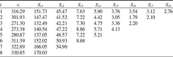
In this section, we apply the MLE approach from Section 3 and the variants from Sections 5 and 6 to the numerical example from Riegel (Reference Riegel2018). Table 1 contains the available volumes (premiums) $v_i$ and the incremental payments $S_{i,k}$ . All figures have been trended to a fixed calendar year. The data are from a large German motor quota share, where claims volatility is low and uncertainty in premium trending is relatively high. In this situation, the premiums provide valuable information about the expected ultimate losses, but the uncertainty in the available volumes should not be ignored.

Table 1.

Premiums and incremental loss triangle.

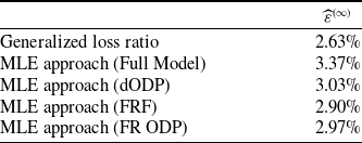
We compare the results of the generalized loss ratio method from Riegel (Reference Riegel2018) with the full MLE approach from Section 3 (Full Model), the distorted dODP from Section 5, and two variants with fixed relativities (FRF and FR ODP) from Section 6. For all approaches, we assume $\lambda_1=\ldots=\lambda_{m-1}=1$ . Table 2 presents the estimators for $\varepsilon$ for all five methods. Note that while the parameter $\varepsilon$ in the generalized loss ratio method has a similar meaning to that in the MLE approaches, it is not identical. Estimating $\varepsilon$ from the data is only reasonable for low-volatility triangles, as in this example.

Table 2.

Estimators for $\varepsilon$ for the generalized loss ratio method and various MLE approaches.

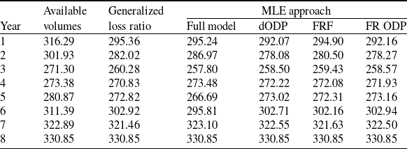
Table 3 shows the premiums $v_i$ , the revised volume estimates $\smash{\widehat{v}_i^{(\infty)}}$ from the generalized loss ratio method and the posterior means $\smash{\widehat{v}_i^{(\infty)}}$ of the latent variables $V_i$ from the MLE approaches.

Table 3.

Available volumes $v_i$ , revised volume estimates $\widehat{v}_i^{(\infty)}$ for the generalized loss ratio method, and posterior means $\widehat{v}_i^{(\infty)}$ of the $V_i$ for various MLE approaches.

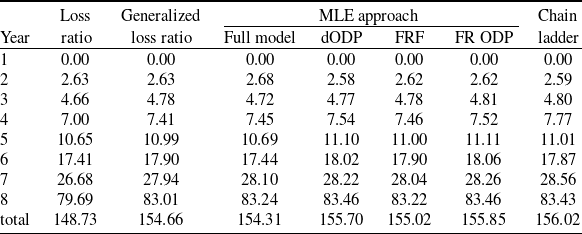
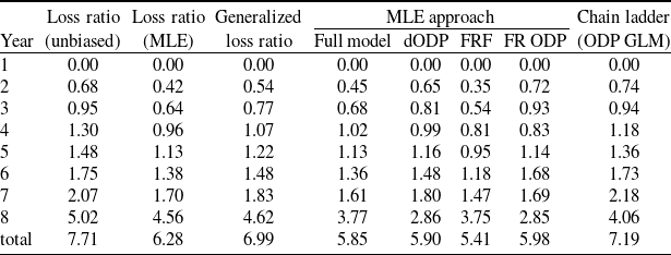
Table 4 compares the predictions of the MLE approaches with the predictions of the classical loss ratio method and the standard chain ladder method. We observe that the predictions of the MLE approach (Full Model) and the FRF approach are quite similar to the predictions of the generalized loss ratio method. The predictions of the dODP and the FR ODP method are slightly closer to the chain ladder results.

Table 4.

Predicted reserves of the considered reserving approaches.

Table 5 provides the standard errors (i.e., the square roots of the MSEP estimates) of the predictions from Table 4.

Table 5.

Standard errors of the considered reserving approaches.

The estimators in the column Loss Ratio (Unbiased) were calculated using the unbiased estimators for $\sigma_k^2$ from Mack (Reference Mack2002), whereas the maximum likelihood estimators $(\widehat{\sigma}^{\mathrm{MLE}}_k)^2$ were used for the column Loss Ratio (MLE). We see that the different estimation principles are the main reason, why the estimated standard errors for the MLE approaches are lower than those of the generalized loss ratio method. The standard errors for the chain ladder method were calculated within the framework of the ODP GLM, using the R package ChainLadder (see Gesmann et al. Reference Gesmann, Murphy, Zhang, Carrato, Wüthrich, Concina and Dal Moro2024).

Additional examples with more volatile datasets are available in the Online Supplementary Material.

8. Conclusions

This paper extends the additive reserving model to address a critical issue in claims reserving when accurate volume measures are unavailable. By proposing a statistical model with latent variables, it provides a practical and computationally efficient alternative to the generalized loss ratio method introduced by Riegel (Reference Riegel2018).

Compared to the classical additive model, the proposed model requires only one additional parameter, $\varepsilon$ , describing the uncertainty of the available volumes. Nevertheless, overparametrization is a critical topic, since, in contrast to the loss ratio method, the predictions are influenced by the estimators of the variance parameters. To address this, two strategies for reducing the number of parameters were explored.

The first strategy employs variance functions, similar to those used in GLMs. While the (distorted) ODP variance structure appeared promising initially, its behavior for $\varepsilon\to 0$ is sometimes counterintuitive, with results that may deviate substantially from the predictions of the additive method.

The second strategy assumes fixed and known relativities between the variance parameters. Variance functions can be used in selecting these relativities, enabling the implementation of different variance structures. This approach aligns with the loss ratio method for $\varepsilon\to 0$ . Additionally, we demonstrated that the corresponding EM iteration has favorable convergence properties for non-singular triangles.

Finally, we applied the methods to a low-volatility Motor example in Section 7. The results closely align with the generalized loss ratio method proposed by Riegel (Reference Riegel2018). Additional examples with higher volatility were considered in the Online Supplementary Material. In the examples, we tested various initial vectors for the EM iteration and did not encounter any convergency issues. In particular, the fixed relativities (FR) variants with variance functions produced stable and intuitive results, even for highly volatile triangles.