

Introduction
Resilience is defined as a positive or successful adaptation in the context of adverse individual, familial or environmental circumstances (see, for example, Rutter, Reference Rutter, Shonkoff and Meissels2000 and Reference Rutter, Clarke-Stewart and Dunn2006; Luthar et al., Reference Luthar, Cicchetti and Becker2000; Masten and Coatsworth, Reference Masten and Coatsworth1998). In other words, resilient individuals have managed to avoid negative outcomes despite (a) being categorised as part of a high risk group, (b) having experienced chronic stress or (c) having been exposed to trauma (Masten et al., Reference Masten, Best and Garmezy1990). Thus resilience moderates (or alters) the response to adversity. As researchers we are interested in identifying those qualities and factors that promote resilience; that enable people to resist and recover from the otherwise negative consequences of adversities.
Regression analyses have been used to uncover patterns of resilience in two different ways. First, resilient factors are sometimes identified and tested by limiting the sample to a high-risk group and identifying those factors that are protective. For example, researchers interested in understanding how children who experienced parental neglect managed to show good psychological adjustment in subsequent years might explore within a sample of neglected children, those factors that are likely to be associated with positive adjustment. When analysing data from a representative sample drawn from the general population, resilient factors can be identified and tested by introducing interaction terms so that adverse risk factors are interacted with factors that may be ameliorative (Roosa, Reference Roosa2000). The researcher could introduce an indicator for parental neglect as a main effect and then interact that variable with another variable, such as an indicator for having good problem solving abilities, that the researcher thinks is likely to be protective.
It is often difficult to resolve whether to regard an observed difference in response to adversity for a measured factor as being indicative of resilience, which identifies the advantaged group, or as a further risk factor, which typically identifies the less advantaged group. Thus, to anticipate our results, we find that those children who had experienced being in care and who were more aggressive (or externalising) were more likely (in combination with other factors) to have no qualifications by age 30. Should we interpret higher aggression as being a risk factor or lower aggression as being a resilience factor? How might we make this distinction? Our view is that such labelling or interpretation is often a matter of the researcher's preference, though sometimes claimed to be for theoretical reasons (i.e. a factor is defined as being a resilience one rather than a risk one). What we see as a key lesson from the resilience approach is a much greater emphasis on the interplays (or interactions) of a range of measures than is usually the case in standard regression models: it is this concept of moderation or the combination of factors that is key.
Parametric approaches like the ones outlined above are good for testing hypotheses about patterns of resilience amongst a select set of variables. However, parametric regression techniques often meet with data constraints on the extent and order of interaction terms. When the number of explanatory variables is large and/or the sample size is not large, researchers interested in studying resilience must choose a priori which interactions to include and test. For many outcomes of interest, the literature can guide researchers in their choice of high-risk groups and factors likely to promote resilience. When this is not the case, researchers may want to apply a method such a Classification and Regression Trees (CART) that can identify interactions directly, either as an end in itself or as a means of choosing amongst different interaction terms to include in regression models.Footnote 1
In this paper, we present the CART method as a means of identifying relationships of resilience and discuss its strengths and weaknesses. To illustrate the method, we use data drawn from the British Cohort Study (BCS70) to construct a classification tree. We use the tree to examine the way in which a variety of childhood risk factors, constructed as summaries of information collected at different childhood waves, are associated with having no academic qualifications at age 30 amongst a group at high risk of social exclusion – those who spent some time in foster care when they were children. Relative to their peers, men and women who have spent time in the care system during childhood fare poorer on a range of outcomes during adulthood, including poor educational achievement (Jackson, Reference Jackson1994). About 26 per cent of our full sample reported having no academic qualifications at age 30, while, amongst those who had been in care, 36 per cent had no qualifications. Poor educational outcomes can lead to poor employment prospects and a higher risk of unemployment and social exclusion (Hobcraft, Reference Hobcraft2000). Indeed, evidence suggests that adults who spent time in care are more likely to be unemployed (Chueng and Heath, Reference Chueng and Anthony1994) and to have experienced homelessness in adulthood (Sigle-Rushton, Reference Sigle-Rushton2004).
Data description
The British Cohort Study (BCS70) is a longitudinal study that attempted to follow the lives of around 16,000 people born during one week in April 1970. The BCS70 conducted interviews shortly after birth, at ages five, ten and 16 during childhood and at ages 26 (a limited postal enquiry), 30 and 34 in adulthood. The sample that we analyse comprises those individuals who had experienced some time in foster care when they were children and for whom our outcome variable, academic qualifications at age 30, is available – a total of 440 individuals.
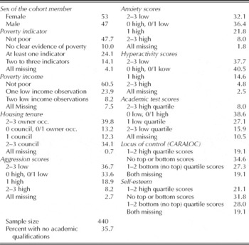
We include a control for the sex of the cohort member. The remaining explanatory variables are, in most cases, constructed as summaries of information collected at more than one childhood wave. However, many cohort members were not interviewed at all ages, and even amongst those who were interviewed there is often a good deal of missing information. Because attrition and non-response appear to be non-random (see Hobcraft, Reference Hobcraft1998; Sigle-Rushton, Reference Sigle-Rushton2004), restricting our sample to those cohort members with complete information could result in serious sample selection issues. We explicitly code missing values for each explanatory variable. Because most of our explanatory variables summarise information collected at various points in time and because we wanted to exploit as much real information as possible, for each summary variable, only those individuals with no information on the characteristic in all of the childhood waves were classified as missing. Those with at least some information were coded into categories that were constructed with some allowance for missing information. This makes use of any information on advantage or disadvantage (even when missing at one or two of the waves) and also permits some measure of intensity, such as depth of childhood poverty. The summary measures of most of the childhood experience variables are documented and more fully described by Sigle-Rushton (Reference Sigle-Rushton2004) following methods developed in Hobcraft (Reference Hobcraft1998, Reference Hobcraft2000). The usual categories were: a group with clear evidence of disadvantage at two or three waves; a group with one piece of evidence of disadvantage, but possibly some information missing at one or two waves; those with no evidence of disadvantage, but with fewer than two indications of advantage; those with two or three indications of advantage; and all information missing. Because information on income, locus of control, and self-esteem was only collected at two childhood waves, there are some minor variations in the categorisation of these measures, as will be apparent from Table 1.
Sample distribution by categories of childhood antecedents for females with information on educational qualifications at age 30 in BCS70

Summary measures of the variables are presented in Table 1. These take comparable inputs at each of the three childhood ages unless otherwise indicated, covering:
• childhood poverty (indicators), as measured by: receipt of free school meals at age ten, receipt of income support or unemployment benefits at age ten and self-assessed financial hardship at age 16;
• childhood poverty (income) using banded family income at ages ten and 16;
• housing tenure, distinguishing renting from local authority (or public housing), owner-occupier and other;
• behavioural measures based on several scale items, taken to represent
aggression,
anxiety, and
restlessness or hyperactivity;
• educational test scores, distinguishing lower and upper quartile scores from intermediate ones;
• locus of control, distinguishing those with at least one bottom quartile or high quartile score (indicating a more internal locus) on the CAROLOC inventory at ages ten and 16;
• and self-esteem, distinguishing those with at least one bottom quartile or high quartile score on the LAWSEQ inventory at ages ten and 16.
These measures provide information on the material resources available during childhood, possible neighbourhood effects, and individual characteristics, some of which have been shown in previous research to be protective (Masten et al., Reference Masten, Best and Garmezy1990; Jackson and Martin, Reference Jackson1994).
Method
The CART method involves repeatedly partitioning the sample into more homogenous groups based on an outcome variable of interest. The results are displayed graphically in tree form and real groups of people in different risk groups can be described and classified. Our summary of the method draws largely from work by Zhang and colleagues (Zhang and Singer, Reference Zhang and Singer1999; Zhang and Bracken, Reference Zhang and Bracken1995). As we describe the way in which trees are constructed and presented, readers might find it useful to refer to Figure 1.
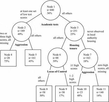
Tree drawn using the BCS70 sample of children who had been in care, pruned to significance level 0.005, showing number of cases, and proportion having no academic qualifications at age 30.

To construct a classification and regression tree, we start with a random outcome variable Y, and a set of p fixed explanatory variables, x 1,x 2,. . .,xp. In what follows, we assume that Y is a dichotomous variable and that some of the x’s contain missing information.Footnote 2 We are interested in identifying the relationship between Y and the x’s so that we can predict Y based on the value of the x’s. Essentially, we want to estimate the probability of the random variable Y conditional on the x’s:

The analysis begins with the unique root node of the tree which is represented by a circle at the top of the tree diagram containing all observations in the sample. At each subsequent layer of the tree, a node can be internal, meaning that additional nodes lie below it, or the node can be terminal, meaning no additional nodes lie below it. Internal nodes are represented with circles and terminal nodes with boxes.
The partitioning technique is applied layer by layer beginning with the root node which is divided into two mutually exclusive left and right ‘daughter’ nodes. We attempt to find a split for each of the two daughter nodes using the same partitioning method, and then their four daughter nodes, on through each layer of the tree. The goal, for each partition, is to locate a binary split that results in two homogeneous, or pure, daughter nodes. Because no split is likely to achieve total purity, we base our choice on a goodness of split measure that weighs the impurities of the resulting daughter nodes. For our estimation, we use the entropy impurity functionFootnote 3 which for node τL is

where p is the proportion of observations with Y = 1 in τL. In order to split a given parent node τ into left and right daughter nodes τL and τR respectively, the goodness of split, s, of node τ is given by

where P{τL} and P{τR} are the probabilities that an observation in the data falls within nodes τL and τR, respectively. We first use the goodness of split measure set out in equation (3) to identify the best split for each predictor variable. The variable with the largest value is chosen to partition that node.
In our application, we utilise the ‘missings together’ approach suggested by Zhang and Singer (Reference Zhang and Singer1999), which for nominal variables treats the missing cases as a single category and for ordinal variables treats those cases with missing information as having either the lowest or the highest value of the variable for which they have missing information. In either case, all of the missing cases are assigned to either τL or τR – possibly as a category by themselves. The ‘missings together’ approach deals nicely with our situation where there is a good deal of missing information in the control variables.
We continue splitting each layer of nodes until the tree is saturated; no offspring nodes can be split any further. Saturated trees are of limited use, statistically, because the terminal nodes are usually very small, and the trees are often so large that interpreting them can be intractable.
In our application, which uses the RTREE software (Zhang et al., Reference Zhang, Holford and Bracken1996),Footnote 4 we make the trees easier to interpret by applying a second step called ‘pruning’. First, we grow the tree until it is saturated. Beginning with the bottom nodes of this tree we begin to prune upwards. To prune the tree, we first calculate a statistic for each internal node from the bottom up. This statistic is the studentized log relative risk of the split to that node, which, for a dichotomous outcome, is the log relative risk that Y = 1 in the two daughter nodes divided by its standard deviation. Next, for each internal node, we compare its statistic with those calculated for all of its offspring nodes. If any offspring node has a higher statistic than its ancestor, we replace the statistic of the ancestor with that higher value. Finally, we examine the size of the statistics for each node. Any node whose statistic falls below some threshold (say 1.96 if we are interested in pruning to a 0.05 significance level) is changed to a terminal node. In practice, this statistic is biased upward, so we use what would normally be a stringent level of significance (0.005) when we prune. The results from the pruned tree identify relationships of resilience when a group of people who are relatively disadvantaged in one domain are (i) split into two groups according to another variable and (ii) those who are less disadvantaged with respect to the splitting variable have a lower risk of experiencing an adverse outcome.
Results
As an illustration of the CART method, we construct a classification tree and use it to explore, amongst those who experienced time in the care system during childhood, relationships between the childhood background factors listed in Table 1 and the outcome of having no academic qualifications at age 30. The tree-based method, pruned to a significance level of 0.005, was applied to our sample (n = 440), the results of which are displayed in Figure 1. In what follows, we describe and discuss this tree with an emphasis on the patterns of resilience it identifies.
At the top of Figure 1, we see that the variable summarising academic test scores was used to split the entire sample (the root node). Two subpopulations result from this split, and comparing nodes 2 and 3, we see that amongst children who had been in care, those who had no low academic test scores were less likely to be unqualified at age 30. The ‘missings together’ approach places those 46 individuals with no test scores at any of the three childhood waves into this lower risk group.
Node 2 is further split via the aggression variable. Amongst those with at least one set of low test scores, those with 2–3 high aggression scores or three missing aggression scores form an extremely high risk group, nearly three-quarters do not have any academic qualifications at age 30. Those with less evidence of aggression are still at heightened risk relative to the root node (45 per cent) but much smaller than that of the left daughter node. Neither of these nodes can be further split and they thus become terminal nodes. Even amongst those with relatively poor educational test scores, a lack of externalising behavioural problems appears to promote resilience possibly by reducing the risk of exclusion from school – a strong correlate of poor educational outcomes (Jackson and Martin, Reference Jackson and Martin1998). Of course the preceding can equally be rephrased as: ‘amongst those with poor educational test scores those who showed clear externalising behavioural problems were at greater risk of lacking qualifications. . .’ .
Node 3 was partitioned using the housing tenure variable, and then subsequently by the locus of control and aggression scores, as can be seen in Figure 1. Amongst those with no low test scores, those who were never observed living in local authority housing during childhood form the lower risk group (node 7) and those with at least one observation in local authority housing as well as those with no information on housing tenure at any of the three childhood waves form the higher risk group, with over double the chances of having no qualification (node 6). In the next layer of the tree, node 6 is further split using the summary of locus of control at ages ten and 16. Amongst those with no low test scores and some experience of living in council housing, having at least one top quartile score on the locus of control inventory is associated with a substantial reduction in the risk of having no academic qualifications. In this node, about 17 per cent of individuals failed to obtain any academic qualifications by age 30. All others are assigned to the higher risk right daughter node, where about half of the individuals failed to do so, three times the risk. Node 7, which contains the most advantaged subset of the sample (those with no low test scores and no evidence of having lived in local authority housing), is further split via childhood aggression. Those with 1–3 high scores form a higher risk left daughter node, and those with no high scores (or all missing) are assigned to the lowest risk group in the tree. For the 140 individuals assigned to this terminal node – about 32 per cent of the sample – only 14 per cent failed to obtain any academic qualification by age 30.
Taken together, the results presented in Figure 1 suggest that amongst those adults who had spent some time in foster care during childhood – a group with a heightened risk of having no qualifications at age 30 – it is possible to identify certain groups that could be labelled as resilient or alternatively their converses which might be labelled high risk. Amongst the group who had any low quartile score (n = 189), the majority (n = 161) have no indications of sustained externalising behaviour problems. About 45 per cent of these cohort members did not obtain an educational qualification by age 30; however, those with lower test scores and repeated externalising problems (n = 28) are at much higher risk of not gaining qualifications, with 75 per cent failing to do so.
The other main split identifies those in our sample who had no indication of a bottom quartile test score. Within this group, two combinations of childhood measures identify groups at low risk of failing to obtain educational qualifications, who might be conceptualized as being resilient: amongst those who did not live in social housing, the larger group (n = 140) with no indication of high aggression (or externalising behaviour problems) were least likely to be unqualified (14 per cent); and amongst those who had any indication of living in social housing, or had no measures of housing tenure, the smaller group (n = 30) who had at least one high quartile indication on the locus of control were also at low risk of being unqualified (17 per cent). The other two groups identified amongst the sample members with no bottom quartile test score were both at considerably higher risk of lacking qualifications and in both cases slightly more likely to lack qualifications than the large group (n = 161) with any bottom quartile test score combined with no severe externalising behaviour (45 per cent): amongst those who had not lived in social housing but had any indication of high childhood aggression (n = 23), 48 per cent lacked qualifications; and amongst those who had lived in social housing, or had tenure missing, but lacked a high quartile measure on the locus of control (n = 58), 50 per cent lacked qualifications. Thus, we effectively pick out three clusters with different propensities to lack qualifications: node 4 identifies a very high risk group (75 per cent); nodes 5, 8, and 10 identify three fairly high risk groups (45 to 50 per cent) and nodes 9 and 11 identify two low risk or resilient groups (14 to 17 per cent).
In order to explore how well the trees identify significant profiles of more and less resilient cohort members, we estimate stepwise logistic models using the same set of explanatory variables and following Hobcraft (Reference Hobcraft1998, Reference Hobcraft2000), entering each as a series of hierarchically defined dummy variables. Taking the most advantaged category as a reference and creating a dummy for the missing value category, we then created a series of dummy variables. The first was set equal to 1 for all categories other than the reference and the missing category. This variable identifies those cohort members for whom there is any possibility of disadvantage as we define it for that variable. The next dummy is set equal to 1 for those members with at least some evidence of disadvantage. A final dummy variable is set equal to 1 only for those with the clearest evidence of disadvantage. This coding strategy allows us to identify splits that are similar to those resulting from the partitioning procedure applied to the nodes of our tree. The only real difference is that our coding strategy treats those with all missing values as a separate category. This deviates to some extent from the ‘missings together’ approach we used when constructing our tree. When the missing category is dropped from the regression, it is implicitly grouped ‘together’ with the reference group. However, when the missing category differs from the reference group, it is treated as a separate variable with a separate parameter and not combined with any dummy variables that are retained.
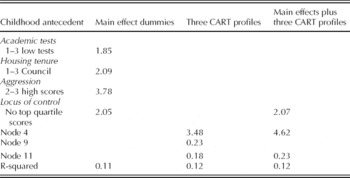
We begin by first estimating a stepwise logistic regression, with backwards elimination and possible re-entry, entering all childhood antecedent dummies as possible covariates. We then re-estimate another model including two indicators for the ‘resilient’ groups (nodes 9 and 11) and the highest risk group (node 4) identified using the CART method.Footnote 5 Finally, we estimate a final stepwise model introducing both sets of covariates. All models are selected using a p-value threshold of 0.01.Footnote 6Table 2 presents results in summary form, showing only the odds ratios for those dummies that were retained in each of the models. In the first column we see that the dummies retained are similar to those used to construct the tree in Figure 1: test scores, aggression, housing tenure and locus of control. In column 2, when the three profiles identified in Figure 1 are introduced as potential covariates all three are retained. The R-squared is similarly sized, suggesting that the tree model summarises the data well, and the profiles identified in Figure 1 do seem to predict a failure to obtain academic qualifications at least as well as models that only allow for main effects amongst the childhood antecedents. Finally in column 3, we find that when both the main effects and the CART profiles are introduced, two of the three node variables are retained (node 4 and node 11) and the locus of control is retained as a main effect. In this particular application, the CART method has revealed combinations of risk or protective factors, or resilience profiles, that would have been difficult to identify using regression methods alone. Elsewhere we have explored further the potential benefits of combining results from classification trees with those from regression models (see Hobcraft and Sigle-Rushton, Reference Hobcraft and Sigle-Rushton2005; also see Zhang and Singer, Reference Zhang and Singer1999).
Odds ratios for significant childhood antecedents of no academic qualifications amongst cohort members who experienced a spell of foster care during childhood (backwards stepwise elimination, p = 0.01)

Discussion and conclusion
In this paper we have presented a method that might help researchers with smaller data sets and a large number of variables to identify patterns of resilience, or at least important combinations of measures associated with differing incidence of outcomes.
Based on our experience with the method, there are two areas (at least) where we have concerns, both of which suggest that this is a method that is best utilised with smaller data sets. First, the binary nature of the splitting leads to quite complex interactions very rapidly. In our illustration, we used a sample with fewer than 500 observations, and nonetheless identified rather complex interaction patterns involving up to three different variables. With larger samples, the pruned trees are often far more complex and become difficult to interpret at even the most stringent levels of significance available with the RTREE software (i.e. 0.0001). Secondly, with larger data sets, we often found only small differences in the impurity and goodness of fit measures, particularly when splitting nodes that lie in the first layers of the tree. As a consequence, nearly every candidate variable provides a competitive split. Even with our smaller data set when splitting the root node, all of the explanatory variables provide competitive splits in the sense that the 95 per cent confidence interval for the relative risk does not contain one. The impurity measures for these variables range from 0.622 to 0.650, suggesting that, given random noise in the data, the choice of best split via this measure might not be as clear-cut as we would like. For this reason, the entire tree may be plagued by high levels of uncertainty. Moreover, small changes in how variables are coded, which could result in small changes in their impurity measures, might nonetheless have large implications for the findings. On the other hand, the option to control the splitting process is useful, however clumsy and limited, and can provide interesting insights into measures that are close competitors and can help researchers to identify relationships between variables that they might not have otherwise considered (Hobcraft and Sigle-Rushton, Reference Hobcraft and Sigle-Rushton2005). The software used, RTREE, does not permit examination of alternative splits within the same variable though and this has posed particular problems when, in the past, we included nominal as well as ordinal variables. However, more sophisticated extensions to so-called ‘random forests’, which consider the likelihood of a variety of trees, have proved successful in the study of tumours when the same subset of predictors appeared in multiple well-fitting trees but sometimes in different orders (Zhang et al., Reference Zhang, Yu and Singer2003).
Despite these caveats, there is considerable advantage to the variables being considered for splitting one at a time which means the option exists to include all sorts of collinear versions of the covariates in a recursive tree analysis. For example, our summary measures of childhood experience regarding each antecedent typically take observations at each of two or three childhood waves and combine them. There is nothing to prevent us including the component measures at each of the three childhood ages as well as the combination in order to explore whether the combination actually does perform better or whether experience at a particular age matters more: for example there is a growing literature that emphasises the importance of early childhood development (e.g. Shonkoff and Phillips, Reference Shonkoff and Phillips2000 and Knudsen et al., Reference Knudsen, Heckman, Cameron and Shonkoff2006). Similarly, the ‘missings together’ approach can be very useful when dealing with the situation we usually face, where the categories for childhood disadvantage on most antecedents are strictly ordered with the exception of those for whom all information is missing; the option to group these in either part of the hierarchy is thus useful.
Although the method is not without problems and appears to be more suitable for some applications than for others, it does offer researchers a flexible and non-parametric way of exploring their data and identifying patterns of resilience (as well as other combinations of measures) that would be difficult to ‘stumble upon’ in the course of estimating regression models. For this reason, CART is a potentially useful methodological tool for researchers who are interested in studying patterns of resilience either as an end in itself or as a preliminary stage and input to more traditional linear regression analyses.