1. Introduction
Since Diamond (Reference Diamond1965), the overlapping generations (OLG) paradigm has become one of the most powerful approaches in the theoretical and applied literature to investigate dynamic economic issues. The OLG model has been used to study several questions regarding economic growth and development (Galor and Ryder, Reference Galor and Ryder1989), population economics (Ehrlich and Lui, Reference Ehrlich and Lui1991; Galor and Weil, Reference Galor and Weil.1996), and infectious diseases (Chakraborty et al. Reference Chakraborty, Papageorgiou and Sebastián2010, Reference Chakraborty, Papageorgiou and Sebastián2016).
Regarding environmental concerns, since John and Pecchenino’s (Reference John and Pecchenino1994) seminal work, which first introduce the interconnection existing between economic activity and environmental quality in an OLG context, many papers have analyzed environmental issues in this setting (e.g., Seegmuller and Verchère, Reference Seegmuller and Verchère2004, Reference Seegmuller and Verchère2007; Antoci and Sodini, Reference Antoci and Sodini2009; Antoci et al. Reference Antoci, Gori and Sodini2016). The success of modeling environmental problems through the OLG model naturally emerges, among other things, from the fact that agents make decisions within a finite lifetime horizon. In this sense, generations do not coordinate themselves, and the presence of a public good (environmental quality) generates problems of private under-investment in the maintenance and/or improvement of the environment. In other words, each generation does not consider the effects of its decisions on the environment that will be inherited by future generations. The line of research referred to in our paper considers environmental quality as a public good that generates a direct flow of welfare to consumers. Typical examples of the benefits of high environmental quality are clean water and clean air (Antoci and Bartolini, Reference Antoci and Bartolini2004). When these resources are degraded due to human activity, their benefits must be replaced by private goods. Textbook examples of this include air filters and water treatment facilities, bottled water, soundproofing, such as double-glazed windows, to mitigate noise pollution from urban traffic, and medications for pollution-related ailments (e.g., asthma and skin conditions). In these instances, individuals are now compelled to purchase goods that were once freely accessible (such as clean air, clean water, quiet surroundings, etc.); by consuming these goods, they endeavor to regain the satisfaction they previously derived from a pristine environment in its original state (i.e., before environmental degradation occurred). This phenomenon of substitution – originally outlined in a seminal work by Hirsch (Reference Hirsch1976) who introduced the notion of “defensive consumption” – extends beyond these textbook examples and has become so prevalent in modern societies that it may contribute to a significant portion of the GDP.
A further feature of these phenomena is that they are characterised by strongly nonlinear relationships, which can give rise to oscillatory dynamics that do not converge to steady states. On this issue, in a relevant paper considering a Cobb-Douglas specification of the John and Pecchenino (Reference John and Pecchenino1994)’s model, Zhang (Reference Zhang1999) showed that the equilibrium dynamics are described by a logistic map, allowing the economy to have a rich spectrum of dynamic outcomes. Similar results have also been obtained in OLG models with a different modeling setting in which agents do not directly invest in environment maintenance but only incur defensive expenditures (Seegmuller and Verchère, Reference Seegmuller and Verchère2007; Antoci and Sodini, Reference Antoci and Sodini2009; Raffin and Seegmuller, Reference Raffin and Seegmuller2014; Antoci et al. Reference Antoci, Gori and Sodini2016).
In addition to the topics just discussed, another issue debated for just over two decades in the OLG context concerns the endogenous choice of technology, which represents a central theme in the theory of economic growth and business cycles. These choices allow for the modeling of how economies can transition between different growth regimes, fall into middle-income or poverty traps, or experience persistent endogenous fluctuations, even of a chaotic nature. Various theoretical contributions have explored this mechanism, highlighting how the nonlinearity introduced by technology selection can generate a rich variety of macroeconomic dynamics. The work of Iwaisako (Reference Iwaisako2002) demonstrated, within an OLG model, how the choice between technologies with different returns to scale can lead to multiple growth trajectories, including endogenous cycles and poverty traps. Subsequently, Matsuyama (Reference Matsuyama2007) introduced financial imperfections and minimum investment sizes, further broadening the spectrum of possible dynamic outcomes. A significant contribution was made by Umezuki and Yokoo (Reference Umezuki and Yokoo2019), who showed that in an OLG model with Cobb-Douglas technologies and log-linear utility, the dynamics reduce to a piecewise linear map on the unit interval. This allows for the rigorous characterization of the existence of periodic cycles of any period, while also demonstrating that non-periodic (chaotic) fluctuations are a “pathological” phenomenon – that is, they occur only for a parameter set of measure zero. However, Asano et al. (Reference Asano, Shibata and Yokoo2024) show that by introducing production externalities (capital externalities), the model can generate observable chaos within a middle-income trap, even with Cobb-Douglas technologies. This occurs when at least one technology exhibits increasing marginal returns, thereby breaking the regularity of the model without externalities. Finally, Asano et al. (Reference Asano, Shibata and Yokoo2023) extend the analysis to the case of CES (Constant Elasticity of Substitution) technologies, demonstrating how the sigmoid shape of the wage function can lead to an even richer variety of development patterns, including chaotic transients and the so-called “pinball effect”, whereby economies with similar initial conditions can diverge towards either high-income or poverty trajectories in an apparently random manner. Collectively, these studies highlight how endogenous technology choice, combined with realistic assumptions such as externalities and nonlinear functional forms, can provide a unified explanation for the coexistence of poverty traps, middle-income traps, perpetual growth, and the complex fluctuations observed in international data.
This paper investigates the role of technological choices on environmental dynamics in an OLG model à la John and Pecchenino (Reference John and Pecchenino1994), following Umezuki and Yokoo (Reference Umezuki and Yokoo2019), and Prieur and Bréchet (Reference Prieur and Bréchet2013), who analyzed an OLG model with physical and (publicly-driven) human capital accumulation. More specifically, the article considers technological choices made in every period by the generation of the firm owners, i.e., the currently living old. Mixing environmental issues (John and Pecchenino, Reference John and Pecchenino1994), physical and human capital dynamics (Prieur and Bréchet, Reference Prieur and Bréchet2013), and rational technology choices (Umezuki and Yokoo, Reference Umezuki and Yokoo2019), which spill over onto the environmental quality and human capital of subsequent generations, cause several macro-dynamics phenomena, in addition to the classic non-coordination problem related to consumption choices and environmental expenditure. From a dynamic point of view, there exist several features that differentiate the present model with models where there is only physical capital accumulation. This is essentially due to the switching between the a physical capital-oriented to a human capital-oriented technology.
The main results of the model show that the interaction between endogenous technological choice and environmental protection decisions generates rich and complex macroeconomic dynamics. Specifically, the model is capable of reproducing a multiplicity of dynamic phenomena, including: (a) the existence of multiple steady-state attractive equilibria (for instance, a “clean” equilibrium with low physical capital intensity and a “polluting” one with high intensity) implying path dependence; (b) the emergence of persistent endogenous fluctuations, including high-period and chaotic dynamics, whether transient or persistent; and (c) border collision bifurcation mechanisms caused by the piecewise nature of the dynamic map, triggered by variations in technological (
 $\alpha _{i}$
) or environmental (
 $ \beta _{i}$
) parameters. These results underscore how the intergenerational conflict and the misalignment of incentives between firm owners (the old) and young workers can lead to suboptimal growth trajectories and significant fluctuations in capital accumulation and environmental quality, highlighting the inefficiency of a purely laissez-faire approach.
From a technical point of view, this work is part of a line of research that has focused on the study of models characterized by the presence of forms of non-derivability or discontinuity in the maps describing their dynamics. In this respect, we recall these characteristics occur in the study of (1) the functioning of financial markets (Tramontana and Westerhoff, Reference Tramontana and Westerhoff2016; Gardini et al. Reference Gardini, Radi, Schmitt, Sushko and Westerhoff2022; Sushko and Tramontana, Reference Sushko and Tramontana2024), (2) the evolutionary dynamics in oligopoly models with bounded rationality (Buccella et al. Reference Buccella, Fanti and Gori2024), (3) the growth cycles in OLG models with perfect foresight (Matsuyama, Reference Matsuyama2007; Asano et al. Reference Asano, Kunieda and Shibata2012, Reference Asano, Shibata and Yokoo2022, Reference Asano, Shibata and Yokoo2023; Asano and Yokoo, Reference Asano and Yokoo2019; Umezuki and Yokoo, Reference Umezuki and Yokoo2019).
The remainder of the article proceeds as follows. Section 2 shows the main features of the model (environmental dynamics, consumers, firms and market-clearing condition). Section 3 analyses the dynamic system emerging when agents select different technologies based on the marginal return. Section 4 concludes the article. Appendix A presents important analytical details of the model. Appendix B considers a brief sketch the optimal policy that a benevolent planner can implement by choosing the tax rate to maximize a social welfare function over time.
2. The model
Building upon the foundational OLG model of environmental economics by John and Pecchenino (Reference John and Pecchenino1994), this paper employs a framework that incorporates public investment in human capital (Glomm and Ravikumar, Reference Glomm and Ravikumar1997), as proposed by Prieur and Bréchet (Reference Prieur and Bréchet2013), and a mechanism of endogenous technological choice (Umezuki and Yokoo, Reference Umezuki and Yokoo2019).
The representative individual born at time
 $t$
has preferences defined over consumption and environmental quality at
 $t+1$
(old age), respectively denoted by
 $C_{t+1}$
and
 $E_{t+1}$
. Preferences are captured by the utility function (see John and Pecchenino, Reference John and Pecchenino1994):
 \begin{equation} U(C_{t+1},E_{t+1})=\ln C{_{t+1}}+\eta \ln {E_{t+1},} \end{equation}
where
 $\eta \gt 0$
measures the relative weight the individual gives to environmental quality against consumption. During the youth, the agent supplies inelastically his time endowment (which is normalized to
 $1$
) to the productive sector receiving a wage per unit of human capital
 $w_{t}$
that he will divide between saving,
 $s_{t}$
(to finance his consumption when old), and investment in environmental maintenance,
 $m_{t}$
(for improving the environmental quality in the future).
Environmental quality is assumed to evolve according to
 \begin{equation} E_{t+1}=(1-b)E_{t}-\beta _{i}C_{t}+\gamma m_{t}, \end{equation}
which strictly follows the environmental dynamic equation introduced by John and Pecchenino (Reference John and Pecchenino1994), where
 $b\in (0,1)$
measures the speed of reversion of the environmental quality to
 $0$
and
 $C_{t}$
is consumption of the generation born at time
 $t-1$
. As in John and Pecchenino (Reference John and Pecchenino1994), the term
 $\beta _{i}C_{t}$
describes the degradation of the environment generated by the consumption activity by the old of the previous generation, where
 $\beta _{i}$
is the time-varying index measuring its impact, which depends on the adopted technology
 $i$
(that will be specified later), and
 $\gamma m_{t}$
measures the environmental improvement chosen by the young of the current generation (those born at time
 $t$
).
The question of whether the environmental index
 $E_{t}$
in this kind of models can represent major, slow-moving natural systems like climate or biodiversity is central to interpreting our results. Based on the structure of our model, which follows the seminal work of John and Pecchenino (Reference John and Pecchenino1994), we argue that the variable
 $E_{t}$
is best interpreted as a measure of environmental quality and ecosystem services rather than a direct proxy for climate or biodiversity. This interpretation is motivated by three key features of the model’s specification.
The law of motion for
 $E_{t}$
, as given by the expression in (2). The parameter
 $b$
measures the speed of reversion to a natural level. A high value of
 $b$
implies a fast regeneration rate. This formulation can characterize environmental goods (e.g., air and water quality, ecosystem health) that can degrade and regenerate relatively quickly due to human activity (
 $C_{t}$
) and investment (
 $m_{t}$
). Climate or biodiversity typically exhibit much longer time lays, higher inertia, and may be subject to tipping points not captured by this linear, mean-reverting process.
The concept of defensive expenditures. As outlined in the introduction, our model builds on the concept of “defensive consumption” (Hirsch, Reference Hirsch1976). The examples provided – such as purchasing air filters, bottled water, soundproofing, and medication for pollution-related ailments – are all reactions to a degradation of immediate environmental conditions. The utility agents derive from
 $E_{t+1}$
represents the enjoyment of these direct, tangible services. This aligns well with environmental quality but is a less direct fit for the more abstract, long-term threats posed by climate change or biodiversity loss, which may not be fully perceptible or compensable through private goods within a single generation’s lifetime.
The generational structure and myopia. A fundamental tenet of the OLG framework applied to the environment (John and Pecchenino, Reference John and Pecchenino1994) is that agents do not internalize the full long-term consequences of their actions on future generations. This myopia is a plausible assumption for environmental problems where the cause and effect are relatively close in time.
Therefore, while our model successfully captures the nonlinear dynamics arising from the interplay between technology choice, economic growth, and environmental protection, the variable
 $E_{t}$
is conceptually and mathematically designed to represent a flow of local environmental services. It is a powerful abstraction for environmental goods that are rival, excludable to some degree, and whose quality can be directly influenced by the defensive actions of a generation within its lifetime.Footnote
1
Going back to the problem, agents supply their savings
 $s_{t}$
to firms earning the expected interest factor
 $R_{t+1}^{e}=1+r_{t+1}^{e}$
, where
 $r_{t+1}^{e}$
is the expected interest rate or the expected return on saving. The representative individual faces the following budget constraints over periods
 $t$
and
 $t+1$
:
 \begin{equation} C_{t+1}=R_{t+1}^{e}s_{t}, \end{equation}
 \begin{equation} (1-\tau )w_{t}H_{t}=s_{t}+m_{t}, \end{equation}
 \begin{equation} C_{t+1},m_{t},s_{t}\geq 0, \end{equation}
where the left-hand side of (4) represents the disposable income of the representative individual when young,
 $H_{t}$
is the level of human capital at time
 $t$
,Footnote
2
i.e., the human capital endowment of the young agent born in period
 $t$
, and
 $0\leq \tau \lt 1$
is the labor income tax rate to finance the activities promoting human capital accumulation.
Substituting the expression in (3) into the utility function for
 $C_{t+1}$
, the representative individual of generation
 $t$
maximizes
 $U$
with respect to
 $s_{t}$
and
 $m_{t}$
, subject to the constraints specified by the expressions in (4), the environmental quality dynamics summarized in (2) and considering the non-negativity constraints in (5).
The constrained utility maximization gives the first order conditions:
 \begin{equation} \frac {R_{t+1}^{e}}{C_{t+1}}=\frac {\gamma \eta }{E_{t+1}}, \end{equation}
that can be rewritten, by using the old-aged budget constraint, as
 \begin{equation} s_{t}=\frac {E_{t+1}}{\gamma \eta }. \end{equation}
From the first-order conditions (which are sufficient due to the concavity of the utility function and linearity of the constraints), one obtains the optimal values of saving and investment in environmental maintenance:
 \begin{equation} s_{t}=\min \left \{ \frac {(1-b)E_{t}-\beta _{i}C_{t}+\gamma (1-\tau )w_{t}H_{t}}{\gamma (1+\eta )},(1-\tau )w_{t}H_{t}\right \} , \end{equation}
and
 \begin{equation} m_{t}=\max \left \{ 0,\frac {\eta (1-\tau )w_{t}H_{t}}{1+\eta }-\frac { (1-b)E_{t}-\beta _{i}C_{t}}{\gamma (1+\eta )}\right \} . \end{equation}
Regarding the supply side, profits of the representative firm at time
 $t$
are defined as
 $\Pi _{t}=Y_{t}-(r_{t}+\delta )K_{t}-w_{t}L_{t}H_{t}$
, where
 $\delta \in \lbrack 0,1]$
is the depreciation rate of capital,
 $r_{t}$
is the real interest rate,
 $w_{t}$
is the wage rate,
 $Y_{t}$
is output and
 $K_{t}$
is the capital input and
 $L_{t}=L=1$
is the labor input. On the production side, unlike the common OLG models, we assume that there are two different Cobb–Douglas technologies with constant returns to scale.
The production function is
 $Y_{t}=\widehat {F}(K_{t},H_{t},L_{t})=AK_{t}^{ \alpha _{i}}(H_{t}L_{t})^{1-\alpha _{i}}=AK_{t}^{\alpha _{i}}H_{t}^{1-\alpha _{i}}, i=\{h,\ell \}$
, which in per worker terms can be written as:
 \begin{equation} y_{t}=\frac {AK_{t}^{\alpha _{i}}H_{t}^{1-\alpha _{i}}}{H_{t}}=Ak_{t}^{\alpha _{i}}, \end{equation}
where
 $A\gt 0$
is the total factor productivity and
 $\alpha _{i}\in (0,1)$
is the capital share of the production of technology,
 $y_{t}=Y_{t}/H_{t}$
(output to human capital ratio) and
 $k_{t}=K_{t}/H_{t}$
(physical to human capital ratio). Let us assume, without loss of generality, that
 $\alpha _{h}\gt \alpha _{\ell }$
. We note that recent empirical literature (Rognlie, Reference Rognlie2015) has shown that the capital share in income has significant variations and oscillations over time, whereas Seegmuller and Verchère (Reference Seegmuller and Verchère2004), in a theoretical model, have found that the capital share in income affects the stationary state equilibria of an overlapping generations model. Based on the capital intensity parameter,
 $\alpha _{i}$
, technology of type
 $h$
represents a traditional, physical capital-intensive production process. A clear example is conventional fossil-fuel-based energy generation, such as a coal-fired power plant. This technology requires a massive initial investment in physical infrastructure (turbines, boilers, generators – high
 $K$
) and is relatively less reliant on a highly specialized workforce for its core operation (lower human capital intensity). As indicated in the introduction, such technologies are typically associated with higher environmental degradation, hence we assign it a higher pollution parameter (
 $ \beta _{h}$
). In contrast, technology of type
 $\ell$
represents a modern, human capital-intensive technology. An example is a renewable energy operation, such as a firm managing a large-scale solar or wind farm. While it still requires significant physical capital (solar panels, wind turbines, land –
 $K$
), its efficiency, innovation, maintenance, and grid integration depend critically on a highly skilled workforce of engineers, data analysts, and technicians (high
 $H$
). This makes it less physically capital-intensive relative to its human capital input. Consistent with the narrative that technological advancement reduces environmental impact, this cleaner technology is associated with a lower pollution parameter (
 $\beta _{\ell }$
). This distinction captures the trade-off of this model. The old generation (firm owners) chooses the technology that maximizes their immediate return on capital,
 $r_{t}$
. This choice has a spillover effect, locking in a specific level of environmental impact for the next period, which affects the utility of the subsequent generation. This intergenerational externality is a core mechanism of the model.
We stress that young agents at time
 $t$
must decide how to allocate their income between savings and environmental maintenance expenditure. These decisions are based on expectations regarding the future interest rate and future environmental quality. However, the choice of production technology for period
 $t$
is made at the beginning of period
 $t$
by firm owners (the elderly of that period) and is not known to young worker agents at time
 $t$
. Specifically: young agents at time
 $t$
know the structural parameters of the model (such as
 $b$
,
 $\gamma$
,
 $\eta$
, etc.), including the
 $\beta _{i}$
value associated with each technology, which is taken as given by agents (consumers) of generation
 $t$
. They form expectations about the interest factor at time
 $t+1$
by assuming that the technological and environmental parameters (
 $\alpha _{i}$
and
 $\beta _{i}$
) remain those of the current period and the production function is given. On the other hand, the technological choice by firm owners (the current period’s elderly) is based on the process of maximizing the return on capital in the current period, thus without internalizing the environmental impact
 $\beta _{i}$
of this choice on future generations. All this captures an intergenerational conflict: the young invest in future environmental quality without having control over the technology that will determine pollution, while the elderly choose technology based on capital returns without concern for environmental externalities.
Profit maximization leads to the following equilibrium conditions (expressed in terms of
 $k_{t}$
):
 \begin{equation} r_{t}=f^{\prime }(k_{t})-\delta =\alpha _{i}Ak_{t}^{\alpha _{i}-1}-\delta , \end{equation}
that equates the gross real interest rate to the marginal productivity of capital, and
 \begin{equation} w_{t}=f(k_{t})-f^{\prime }(k_{t})k_{t}=(1-\alpha _{i})Ak_{t}^{\alpha _{i}}, \end{equation}
that equates the wage rate to the marginal productivity of human capital based labor.
We assume that, at the beginning of every period, firm owners (i.e., the old born at the beginning of the previous period) consider a discrete-choice problem regarding technology selection (Umezuki and Yokoo, Reference Umezuki and Yokoo2019) by choosing the technology leading to the highest return at time
 $t$
(as it is expressed in Eq. (11)).Footnote
3
Given the production function defined in (10), owners will choose the technology with a lower (resp. higher) value of
 $ \alpha$
if
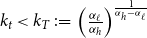 $k_{t}\lt k_{T}\;:\!=\;\left ( \frac {\alpha _{\ell }}{\alpha _{h}}\right ) ^{\frac {1}{\alpha _{h}-\alpha _{\ell }}}$
(resp.
 $k_{t}\gt k_{T}$
), where
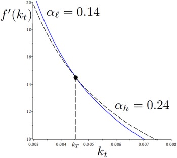
 $k_{T}$
represents a threshold value of
 $k_{t}$
where the two technologies have the same marginal returns (see Figure 1). The figure shows marginal return on capital associated to
 $\alpha _{\ell }$
and
 $\alpha _{h}$
, i.e.,
 $ f^{\prime }(k_{t})=\alpha _{\ell }Ak_{t}^{\alpha _{\ell }-1}$
and
 $f^{\prime }(k_{t})=\alpha _{h}Ak_{t}^{\alpha _{h}-1}$
, respectively, when
 $k_{t}$
varies. The former is represented by the solid blue line in and the latter by the black dashed line.
These choices have an impact on the environment and its dynamics. We note that
 $\beta _{i}$
is not internalized by the currently living old agents as its level will affect the utility of the next generation.
In this regard, we stress that we are implicitly considering modern economies in which technological advancement (and higher human capital accumulation) leads to a reduction in environmental impact, as opposed to what might have been observed in earlier historical phases.
Marginal returns on capital for two different levels of
 $\alpha _{i}$
. The solid blue line refers to
 $\alpha _{\ell }$
. The black dashed line refers to
 $\alpha _{h}$
.

To simplify the analysis, we assume education services are provided by public facilities and financed through labor income taxes levied on consumers, as in Glomm and Ravikumar (Reference Glomm and Ravikumar1997). This is to avoid adding an additional control variable on the individual side about private choices in education. Then, as in Prieur and Bréchet (Reference Prieur and Bréchet2013), we consider the following law of motion of human capital accumulation:
 \begin{equation} H_{t+1}=H_{t}\cdot g(x_{t}), \end{equation}
where
 $g(\!\cdot\!)$
is a function of
 $x_{t}\;:\!=\;X_{t}/H_{t}\geq 0$
representing the public-financed expenditure in education to human capital ratio at time
 $ t$
. The total public expenditure
 $x_{t}H_{t}$
is financed at balanced budget in each period. Then, the budget constraint of the government at time
 $t$
is given by:
 \begin{equation} x_{t}H_{t}=\tau H_{t}w_{t}\Longrightarrow x_{t}=\tau w_{t}. \end{equation}
We define the function
 $g$
as follows
 \begin{equation} g(x_{t})=(z+x_{t})^{\phi }, \end{equation}
with
 $\phi \in (0,1)$
and
 $z\geq 0$
is a constant. We note that (15) satisfies some of the properties in Assumption 2 of Prieur and Bréchet (Reference Prieur and Bréchet2013, p. 1139), that is the function is increasing and concave in
 $x_{t}$
,
 $x_{t}\geq 0$
. Unlike Prieur and Bréchet (Reference Prieur and Bréchet2013), however, we do not impose
 $g(0)=0$
, but we have that when
 $z\gt 0$
then
 $g(0)\gt 0$
. Using Eqs. (13)–(15), the human capital accumulation equation can be re-written as follows:
 \begin{equation} H_{t+1}=H_{t}\cdot \lbrack z+\tau (1-\alpha _{i})Ak_{t}^{\alpha _{i}}]^{\phi }. \end{equation}
Let us now examine in detail the role of
 $z$
introduced in (15) in the dynamics of human capital accumulation. If
 $z=0$
, in the absence of the public expenditure in education the stock of human capital goes to zero in one period from which production becomes null (as in Prieur and Bréchet, Reference Prieur and Bréchet2013). If
 $z\in (0,1)$
, the stock of human capital tends to zero without public expenditure unless there is a sufficiently high amount of investment in education. If
 $z=1$
, human capital remains constant if public expenditure is zero. If
 $z\gt 1$
, there exists an exogenous process that increases human capital regardless of public spending.
The market-clearing condition in the physical capital market requires
 $ K_{t+1}=s_{t}$
, which can be rewritten as
 \begin{equation} k_{t+1}H_{t+1}=s_{t}. \end{equation}
Considering the relationship between the state variables from the consumer’s problem (interior solution), (7), and Eq. (17), one obtains:
 \begin{equation} E_{t+1}=\gamma \eta k_{t+1}H_{t+1}. \end{equation}
So, at a stationary state of the variable
 $k$
, the states
 $E$
and
 $H$
grow at the same rate. Given the definition of
 $k$
, the level of physical capital also grows at the same rate as the other two state variables.
The following expressions hold at the interior optimum:
 \begin{equation} C_{t}=(1+\alpha _{i}Ak_{t}^{\alpha _{i}-1}-\delta )k_{t}H_{t}, \end{equation}
and
 \begin{equation} m_{t}=(1-\tau )(1-\alpha _{i})Ak_{t}^{\alpha _{i}}H_{t}-k_{t+1}H_{t+1}. \end{equation}
Substituting (18) and (19) into (8) we get the following one-dimensional piecewise continuous dynamic system:
 \begin{equation} k_{t+1}=T(k_{t})\;:\!=\;\left \{ \begin{array}{c} p_{1}(k_{t})=\frac {[(1-\alpha _{\ell })(1-\tau )\gamma -\beta _{\ell }\alpha _{\ell }]Ak_{t}^{\alpha _{\ell }}-\left [ \beta _{\ell }(1-\delta )-(1-b)\gamma \eta \right ] k_{t}}{\gamma (1+\eta )[z+A\tau (1-\alpha _{\ell })k_{t}^{\alpha _{\ell }}]^{\phi }}\text{ if }k_{t}\lt k_{T} \\ p_{2}(k_{t})=\frac {[(1-\alpha _{h})(1-\tau )\gamma -\beta _{h}\alpha _{h}]Ak_{t}^{\alpha _{h}}-\left [ \beta _{h}(1-\delta )-(1-b)\gamma \eta \right ] k_{t}}{\gamma (1+\eta )[z+A\tau (1-\alpha _{h})k_{t}^{\alpha _{h}}]^{\phi }}\text{ if }k_{t}\gt k_{T} \end{array} \right . . \end{equation}
If
 $\phi =0$
, our model reduces to Zhang’s model by appropriately rescaling the parameters. Once the dynamics of
 $k$
are defined, the dynamics of
 $H$
can be calculated from Eq. (16) whereas the dynamics of
 $E$
easily follows from the expression in (18).
To simplify the exposition, let us introduce two new parameters:
 $\widetilde { A}=[(1-\alpha _{i})(1-\tau )\gamma -\beta _{i}\alpha _{i}]A$
and
 $\widetilde { B}=\beta _{i}(1-\delta )-(1-b)\gamma \eta$
. On the one hand,
 $\widetilde {A}$
captures the relationships between the elements that determine the impacts of agents’ decisions on environmental dynamics (
 $\beta _{i}$
and
 $\gamma$
) and technological parameters (
 $A$
and
 $\alpha _{i}$
), as well as the “weight” of public intervention (
 $\tau$
). Given its definition,
 $\widetilde {A}$
can be either positive or negative. In particular,
 $\widetilde {A}\gt 0$
(resp.
 $\lt 0$
) is favored by sufficiently low (resp. high) values of
 $\alpha _{i}$
,
 $\beta _{i}$
and
 $\tau$
and high (resp. low) values of
 $\gamma$
. On the other hand,
 $\widetilde {B}$
captures relationships between the elements that define environmental dynamics (
 $ \beta _{i}$
,
 $\gamma$
and
 $b$
) and the parameters that define the individual decisions of the agents (
 $\delta$
and
 $\eta$
). Also, the parameter
 $\widetilde {B}$
can be positive or negative and a positive (resp. negative) value is favored by high (resp. low) values of
 $\beta _{i}$
and
 $ b$
and low (resp. high) values of
 $\delta$
,
 $\gamma$
, and
 $\eta$
.
Importantly, by changing
 $\alpha _{i}$
,
 $\tau$
, and
 $A$
in
 $\widetilde {A}$
(parameters that do not appear in
 $\widetilde {B}$
), we have that
 $\widetilde { A}$
can vary in the interval
 $(\!-\!\infty ,\infty )$
leaving the value of
 $\widetilde {B}$
unchanged. Unlike this,
 $\widetilde {B}$
can vary in the interval
 $ (\!-\!\infty ,\beta _{i}(1-\delta ))$
through the parameter
 $\eta$
leaving the value of
 $\widetilde {A}$
unchanged.
3. Dynamics of the model
Before analyzing the endogenous choice of
 $\alpha _{i}$
and
 $\beta _{i}$
, let us consider some basic properties of the model with constant values of these parameters.
3.1 The model with no endogenous technological choice
Let us first consider the case
 $\widetilde {A}\gt 0$
. Then, the following propositions hold.
Proposition 1.
Let
 $\alpha _{i}=\alpha$
,
 $\ \beta _{i}=\beta$
,
 $ i=\{h,\ell \}$
and
 $\widetilde {A}\gt 0$
. Then, map
 $T(k_{t})$
always admits a positive fixed point,
 $k^{\ast }$
.
Proof.
Dividing both sides of (21) by
 $k$
the search for fixed points is equivalent to finding positive solutions to the equation
 \begin{equation} 1=n(k)\;:\!=\;\frac {\widetilde {A}k^{\alpha -1}-\widetilde {B}}{\gamma (1+\eta )[z+A\tau (1-\alpha )k^{\alpha }]^{\phi }}, \end{equation}
that is, the value of
 $k\gt 0$
where the graph of the function
 $q=n(k)$
intersects the horizontal line
 $q=1$
. This intersection must occur for a value of
 $k$
in which the numerator of
 $n(k)$
is positive. Differentiating
 $ n(k)$
we obtain the following expression:
 \begin{equation} n^{\prime }(k)=\frac {-A\tau \phi (1-\alpha )\alpha k^{\alpha -1}(\widetilde {A }k^{\alpha -1}-\widetilde {B})[z+A\tau (1-\alpha )k^{\alpha }]^{-1}- \widetilde {A}(1-\alpha )k^{\alpha -2}}{\gamma (1+\eta )[z+A\tau (1-\alpha )k^{\alpha }]^{\phi }}, \end{equation}
which is negative for all
 $k$
where the numerator of
 $n(k)$
is positive. Notice that if
 $\widetilde {B}\gt 0$
then
 $\left . n(k)\right \vert _{k=( \widetilde {A}/\widetilde {B})^{1/(1-\alpha )}}=0$
, while if
 $\widetilde {B}\lt 0$
then
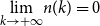 $\underset {k\rightarrow +\infty }{\lim }n(k)=0$
. As
 $n$
is monotonically decreasing and
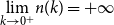 $\underset {k\rightarrow 0^{+}}{\lim } n(k)=+\infty$
and
 $\left . n(k)\right \vert _{k=(\widetilde {A}/\widetilde {B} )^{1/(1-\alpha )}}=0$
, a positive fixed point exists and it is unique.
Proposition 2.
Let
 $\alpha _{i}=\alpha$
and
 $\beta _{i}=\beta$
,
 $ i=\{h,\ell \}$
. If
 $\widetilde {A}\gt 0$
and
 $\widetilde {B}\lt 0$
then map
 $T(k_{t})$
is monotonically increasing and the dynamics with
 $k_{0}\gt 0$
are monotonic and converging towards the unique positive fixed point.
Proof.
As
 $\widetilde {A}\gt 0$
the interior equilibrium exists and is unique. The result is obtained by considering the first derivative of (21), that is:
 \begin{equation} T^{\prime }(k_{t})=\frac {-\widetilde {B}k_{t}[z+A\tau (1-\alpha )(1-\alpha \phi )k_{t}^{\alpha }]+\widetilde {A}A\tau \alpha (1-\alpha )(1-\phi )k_{t}^{2 \alpha }+z\widetilde {A}\alpha k_{t}^{\alpha }}{\gamma (1+\eta )k_{t}[z+A\tau (1-\alpha )k_{t}^{\alpha }]^{1+\phi }}. \end{equation}
For
 $\widetilde {A}\gt 0$
, the following results hold at the fixed point
 $ k^{\ast }$
, regardless of the sign of
 $\widetilde {B}$
.
Proposition 3.
Let
 $\widetilde {A}\gt 0$
,
 $\alpha _{i}=\alpha$
,
 $ \beta _{i}=\beta$
,
 $i=\{h,\ell \}$
hold, and
 $k^{\ast }=k^{\ast }(\alpha ,\beta ,\gamma ,\delta ,\eta ,\tau ,\phi ,A,b)$
. We have the following results.
 $\frac {\partial k^{\ast }}{\partial \beta }\lt 0$
,
 $\frac {\partial k^{\ast }}{ \partial \gamma }\gt 0$
,
 $\frac {\partial k^{\ast }}{\partial \delta }\gt 0$
,
 $\frac { \partial k^{\ast }}{\partial \eta }\gt 0$
,
 $\frac {\partial k^{\ast }}{\partial \tau } \lt 0$
,
 $\left . \frac {\partial k^{\ast }}{\partial \phi }\right \vert _{z\geq 1}\lt 0$
,
 $\frac {\partial k^{\ast }}{\partial A}\gt 0$
and
 $\frac {\partial k^{\ast }}{ \partial b}\lt 0$
.
Proof.
The results can be verified by applying the implicit function theorem to the stationary condition
 $T(k)=k$
.
The role of
 $\phi$
and
 $z$
on
 $k^{\ast }$
is ambiguous. These results are not merely mathematical curiosities but stem from the model’s core structure. The ambiguity arises from the dual, and often opposing, effects these parameters have on the production function and the human capital accumulation function at different levels of development. The ambiguous effect of the human capital elasticity (
 $\phi$
) is contingent on the autonomous growth factor (
 $z$
). A higher
 $\phi$
makes human capital more responsive to public investment. If
 $z\geq 1$
, the economy has a strong baseline human capital growth. In this case, further enhancing the returns to education spending (a higher
 $\phi$
) can lead to a relative abundance of human capital (
 $H_{t}$
) compared to physical capital (
 $K_{t}$
), thus reducing the physical to human capital ratio
 $k^{\ast }$
. However, if
 $z\lt 1$
, the system is more fragile and reliant on public investment. Here, a higher
 $ \phi$
can powerfully stimulate human capital accumulation, but it may also require a parallel accumulation of physical capital to equip the more highly skilled workforce, potentially increasing
 $k^{\ast }$
. The net effect is ambiguous and depends on the specific parameter constellation. Similarly, a higher capital share (
 $\alpha$
) has two countervailing effects. On the one hand, it directly increases the marginal product of capital, incentivising greater capital accumulation, which tends to increase
 $k^{\ast }$
. On the other hand, a higher
 $\alpha$
implies a lower labor share, which reduces wage income. Since wages fund the savings that become next period’s capital, this can suppress capital accumulation. Furthermore, lower wages mean lower tax revenues for public education (
 $x_{t}=\tau w_{t}$
), potentially slowing human capital (
 $H_{t}$
) growth, which would mechanically increase the ratio
 $ k_{t}=K_{t}/H_{t}$
. The ultimate impact on the steady-state ratio
 $k^{\ast }$
is therefore a complex balance of these direct and indirect, positive and negative, channels. This interaction underscores that the relationship between policy levers (like investment in education, which influences
 $\phi$
and
 $z$
indirectly) and economic outcomes is highly context-dependent, varying with the economy’s existing capital structure and institutional setup.
Regarding the growth rate of human capital, in correspondence of
 $k^{\ast }$
, denoted by
 $g_{H}(k^{\ast })$
, it is positively affected by
 $\gamma$
,
 $ \delta$
,
 $\eta$
and
 $A$
and negatively by
 $\beta$
. A change in the other parameters can either increase or decrease
 $g_{H}(k^{\ast })$
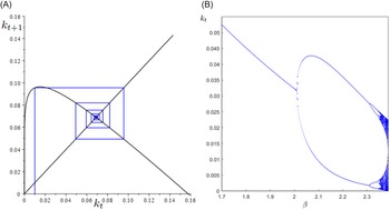
. It is important to note that, also in the absence of technology switches, the model dynamics can be non-monotonic. Temporary (Figure 2A) or persistent (Figure 2B) oscillations occur only if
 $\widetilde {A}\gt 0$
and
 $\widetilde {B}\gt 0$
. As in this case the map is not monotonic, to ensure well-defined dynamics for every initial condition, one must impose that at the maximum point
 $k_{\max }$
the image of this point is not greater than
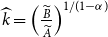 $\widehat {k}=\left ( \frac {\widetilde {B}}{{^{^{^{^{^{\!}}}}}}\widetilde {A}}\right ) ^{1/(1-\alpha )}$
, where the map
 $T$
is zero. Although an explicit expression for
 $k_{\max }$
cannot be obtained, it can be deduced, under the assumptions
 $\widetilde {A}\gt 0$
and
 $\widetilde {B}\gt 0$
, that such a point exists, is unique and
 $0\lt k_{\max }\lt \widehat {k}$
. The threshold
 $\widehat {k}$
also represents the upper bound for the initial condition of
 $k_{t}$
to have dynamics defined by an interior solution of the agent problem, i.e.
 $m_{t}\gt 0$
. Unlike models in which the dynamics of
 $K_{t}$
is directly considered, and thus it makes economic sense to account for an initial condition of
 $K_{t}$
less than the stationary value of
 $K$
, in the present model it can also be meaningful studying the dynamics of
 $k_{t}$
(which is the physical capital to human capital ratio) with initial conditions greater than
 $k^{\ast }$
. In this case, if
 $k_{0}\gt k^{\ast }$
and
 $k^{\ast }$
is an attractor with
 $ T^{\prime }(k^{\ast })\in (0,1)$
, the dynamics will converge to
 $k^{\ast }$
with decreasing
 $k_{t}$
. Thus, during the transition, the growth rate of human capital (
 $H$
) will be greater than the growth rate of physical capital (
 $K$
). About the stability conditions of
 $k^{\ast }$
we can infer, at least numerically, that starting from a stable situation an increase in
 $\beta$
can induce a destabilization of the equilibrium (as shown in Figure 2B). In addition, the role of
 $\alpha$
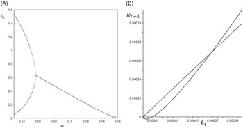
on stability is ambiguous, as shown in Figure 3A.
Parameter set:
 $A=1$
,
 $b=0.7$
,
 $\gamma =0.79$
,
 $\tau =0.41$
,
 $\eta =0.04$
,
 $\delta =0.4$
,
 $z=1$
,
 $\phi =0.5$
and
 $\alpha =0.144$
. (A) Damping oscillations (
 $\beta =1.5$
). (B) Bifurcation diagram for
 $\beta$
(ranging from
 $2.7$
to
 $2.4$
).

Considering now the case
 $\widetilde {A}\lt 0$
, if
 $\widetilde {B}\gt 0$
then the dynamics are unfeasible as the map implies
 $k_{1}\lt 0$
given any initial value of
 $k_{0}$
; if
 $\widetilde {B}\lt 0$
then the map can have zero or two fixed points (see Eq. (23)). When two fixed points exist,
 $k_{1}^{\ast }$
being the first between them, the initial value of
 $k$
must be greater than
 $k_{1}^{\ast }$
to ensure
 $m_{t}\gt 0$
(see Figure 3B). In terms of the corresponding level of the variables involved, this means that there must be a relative abundance of physical capital
 $K$
compared to human capital
 $H$
at the beginning of time.
(A) Bifurcation diagram for
 $\alpha$
. (B) Case
 $\widetilde {A}\lt 0$
and
 $\widetilde {B}\lt 0$
. Parameter set:
 $A=0.12$
,
 $ b=0.81$
,
 $\gamma =1.079$
,
 $\tau =0.91$
,
 $\eta =0.094$
,
 $\delta =0.9$
,
 $\phi =0.99$
,
 $\alpha =0.8$
,
 $\beta =0.04$
and
 $z=0.004$
.

3.2 The model with endogenous technological choice
Let us now consider the case in which technology decisions are endogenous. It can be verified that the change from the piece
 $p_{1}(k_{t})$
to the piece
 $p_{2}(k_{t})$
at
 $k_{T}$
can cause a downward or an upward jump in the map. During a phase of increasing
 $k_{t}$
, a switch from
 $p_{1}(k_{t})$
to
 $p_{2}(k_{t})$
causing an upward (resp. downward) jump implies an increase (resp. a decrease) in the difference between the growth rates of (the level of) physical capital (
 $K$
) and (the level of) human capital (
 $H$
). Similar considerations apply in a decreasing phase of
 $k_{t}$
when a switch from
 $p_{2}(k_{t})$
to
 $p_{1}(k_{t})$
occurs.
Parameter set:
 $A=0.12$
,
 $b=0.81$
,
 $\gamma =1.079$
,
 $\tau =0.91$
,
 $\eta =0.094$
,
 $\delta =0.9$
,
 $z=0.006$
,
 $\phi =0.99$
,
 $\beta _{h}=0.03$
,
 $\alpha _{h}=0.5$
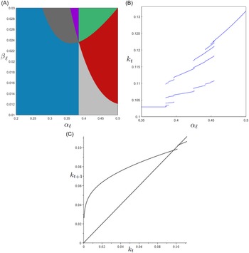
. (A) Geometrical portrait of the scenarios from Proposition 4. Blue: only one fixed point (in the second piece of the map) and downward jump. Light gray: no fixed point and downward jump. Dark gray: only one fixed point (in the second piece of the map) and upward jump. Violet: two fixed points, one per piece, and upward jump. Red: only one fixed point (in the first piece of the map) and downward jump. Green: only one fixed point (in the first piece of the map) and upward jump (
 $\alpha _{\ell }\in \lbrack 0.2,\alpha _{h}]$
and
 $\beta _{\ell }\in \lbrack 0.01,\beta _{h}]$
). (B) Bifurcation diagram for
 $ \alpha _{\ell }$
(
 $\alpha _{\ell }\in \lbrack 0.35,\alpha _{h}]$
and
 $\beta _{\ell }=0.014$
). (C) Multiple attracting fixed points (
 $\alpha _{\ell }=0.38$
and
 $\beta _{\ell }=0.029$
).

The analysis of the piecewise map
 $T(k_{t})$
, particularly how the two branches
 $p_{1}(k_{t})$
and
 $p_{2}(k_{t})$
behave at the threshold
 $k_{T}$
, allows us to study the direction and magnitude of the “jump” at
 $k_{T}$
(upward or downward), and the number and location of fixed points in each region (
 $k\lt k_{T}$
and
 $k\gt k_{T}$
). The results are summarized in the following proposition.
Proposition 4.
Let
 $T$
be the map defined in (
21
) and
 $(1-\alpha _{\ell })(1-\tau )\gamma -\beta _{\ell }\alpha _{\ell }\gt 0$
. The following scenarios hold. (a) If (a.1)
 $\ p_{1}(k_{T})\gt p_{2}(k_{T})\gt k_{T}$
or (a.2)
 $\ p_{2}(k_{T})\gt p_{1}(k_{T})\gt k_{T}$
then one positive fixed point
 $k^{\ast }$
exists and
 $k^{\ast }\gt k_{T}$
. (b) If
 $p_{1}(k_{T})\gt k_{T}\gt p_{2}(k_{T})$
and
 $ p_{2}(k_{T})\gt 0$
then no fixed points exist. (c) If
 $ p_{2}(k_{T})\gt k_{T}\gt p_{1}(k_{T})$
then two fixed points
 $k_{1}^{\ast }$
and
 $ k_{2}^{\ast }$
exist with
 $k_{1}^{\ast }\lt k_{T}\lt k_{2}^{\ast }$
. (d) If (d.1)
 $ \ k_{T}\gt p_{1}(k_{T})\gt p_{2}(k_{T})$
and
 $p_{2}(k_{T})\gt 0$
or (d.2)
 $\ k_{T}\gt p_{2}(k_{T})\gt p_{1}(k_{T})$
then one positive fixed point
 $k^{\ast }$
exists and
 $k^{\ast }\lt k_{T}$
.
Proof.
The proof follows from evaluating
 $p_{1}(k_{t})$
and
 $p_{2}(k_{T})$
at the extremes of their domain of definition.
Proposition 4 does not rule out cases in which
 $(1-\alpha _{h})(1-\tau )\gamma -\beta _{h}\alpha _{h}\lt 0$
. From an economic point of view, in an economy using physical capital intensive technology, this means that we cannot exclude that positive solutions for
 $m_{t}$
require a sufficiently high level of
 $K$
. Figure 4A illustrates a case where all scenarios characterized in Proposition 4 are possible, with
 $p_{1}(k_{t})$
and
 $p_{2}(k_{t})$
both increasing as
 $\alpha _{\ell }$
and
 $\beta _{\ell }$
change. These are the parameters representing the technological and environmental characteristics, respectively, when the more human capital-intensive technology is selected.Footnote
4
From Figure 4A, we observe that by varying
 $\alpha _{\ell }$
in the interval
 $(0.2,0.5)$
we move from a situation in which there is only one fixed point defined by the first piece of the map, which captures all initial conditions, to a case in which the dynamics converge to cycles of different periods born through border collision bifurcations (see Figure 4B) turning back, by increasing the value of
 $\alpha _{\ell }$
further, to a case in which the global attractor is a fixed point defined by the second piece of the map. More specifically, Figure 4A, classifies the dynamic regimes of the system in the
 $(\alpha _{\ell },\beta _{\ell })$
-space, based on Proposition 4. Each color corresponds to a distinct regime (e.g., one fixed point, two fixed points, etc.). Panels B and C illustrate specific dynamic behaviors along a slice of this parameter space. In Panel B, we fix
 $\beta _{\ell }=0.014$
and vary
 $\alpha _{\ell }\in \lbrack 0.35,0.5]$
. The bifurcation diagram shows how the system undergoes border collision bifurcations and transitions into chaotic regimes as
 $\alpha _{\ell }$
increases, corresponding to traversing the violet and dark gray regions in Panel A. In Panel C, for
 $\alpha _{\ell }=0.38$
and
 $\beta _{\ell }=0.029$
(violet region), two fixed points coexist, demonstrating path dependence. These examples highlight how the global dynamics emerge from the piecewise structure of the map and the endogenous technology choice.
Due to the optimizing process, the feedback from individual decisions on the evolution of environmental quality, and also the public funding of education expenditure, several other mechanisms may contribute to the emergence of cycles. In particular, as it is possible for both pieces of the map to have decreasing branches or to be uni-modal, cycles may be generated from the destabilization by a flip bifurcation of a fixed point in one of the two pieces of the map. Depending on the parameters of the model, oscillations may involve one or both pieces of the map. In addition, multiple high-period cycles or even chaotic attractors may coexist.
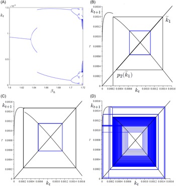
To illustrate some of the phenomena described so far, let us consider the bifurcation diagram in Figure 5A. The analysis shows that, starting from a situation where the dynamics are attracted to a fixed point defined by
 $p_{2}(k)=k$
(agents always select the most environmentally harmful technology), an increase in
 $\beta _{h}$
causes the dynamics to converge to a
 $2$
-period cycle
 $\bar {k}_{1}$
and
 $\bar {k}_{2}$
with
 $k_{T}\lt \bar {k} _{1}\lt \bar {k}_{2}$
(see Panel B of Figure 5). From the bifurcation diagram, we note a discontinuity at
 $\beta _{h}\cong 1.646$
and at
 $\beta _{h}\cong 1.714$
an abrupt enlargement of this attractor for
 $\beta _{h}=1.72$
. The comparison of Panels B–D of Figure 5 explains these mechanisms in detail. We begin by noting that for the selected parameter set and for
 $ \beta _{h}\in (1.6,1.72)$
,
 $p_{2}$
is always decreasing on the interval
 $ (k_{t},k_{f})$
, where
 $k_{f}$
is the positive value for which
 $ p_{2}(k_{f})=0$
. In addition,
 $p_{1}$
has a maximum at a point
 $\widehat {k} _{\max }$
where
 $0\lt \widehat {k}_{\max }\lt k_{T}$
.
For convenience, we introduce the following values:Footnote
5
 $\widetilde {k} _{1}\;:\!=\;p_{2}(k_{T}),$
and
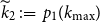 $\widetilde {k}_{2}\;:\!=\;p_{1}(k_{\max })$
. In Panel B of Figure 5, we have that (a)
 $\widetilde {k}_{1}\gt 0$
and
 $p_{2}(\widetilde {k} _{1})\gt k_{T}$
(see the black segment line depicted in bold in the center of the figure on the
 $45^\circ$
line), and (b) there exists
 $n\in \mathbb{N}$
sufficiently high such that
 $p_{1}^{n}(0,k_{f})\subset I=(p_{2}(\widetilde {k}_{1}),\widetilde {k}_{1})$
. This means that the segment
 $I\subset (k_{T},k_{f})$
is an absorbing interval, i.e. the forward dynamics of the map will sooner or later end up in
 $I$
and will not exit from there. Therefore, after a possible switching phase between the two technologies, the technology selected will be the one associated with
 $\alpha _{h}$
. Specifically in Figure 5, Panel B, the dynamics converge to a
 $2$
-period cycle (depicted in blue).
An increase in
 $\beta _{h}$
makes
 $k_{2}$
and its subsequent iterates no longer fall into
 $I$
, although
 $I$
remains an absorbing interval. In other words, there will exist a set of initial conditions belonging to
 $(0,k_{f})$
with different fate. At this stage, as shown in Panel C of Figure 5, two attractors coexist (depicted in black and blue). Thus, initial conditions can lead to trajectories with different environmental and economic features, even in the long term. The discontinuity in the bifurcation diagram occurs because the chosen initial condition
 $k_{0}\lt k_{T}$
is now in the basin of the attractor not contained in
 $I$
. Then, the discontinuity in the bifurcation diagram occurs because the initial condition
 $k_{0}\lt k_{T}$
is now in the basin of the attractor not in
 $I$
.
Due to the changes on
 $p_{2}$
induced by
 $\beta _{h}$
for
 $\beta _{h}\in (1.714,1.717)$
, the
 $2$
-period cycle on
 $I$
turns out to be the only attractor of the system after a contact between the basins of attraction of the two attractors. A further increase in
 $\beta _{h}$
shifts the point
 $ (p_{2}(\widetilde {k}_{1}))$
to the left until
 $p_{2}(\widetilde {k} _{1})\lt k_{T}$
. This makes the segment
 $I$
no longer forward invariant. Then, even the dynamics arising from
 $I$
will no longer be confined to
 $I$
, but will develop more generally on the set
 $(p_{1}(\widetilde {k}_{2}),\widetilde { k}_{2})$
(at least until
 $p_{1}(\widetilde {k}_{2})\gt 0$
), as illustrated in Panel D of Figure 5.
(A) Bifurcation diagram for
 $\beta _{h}$
.
 $ A=0.02$
,
 $b=0.29$
,
 $\gamma =0.78$
,
 $\tau =0.5$
,
 $\eta =0.06$
,
 $\delta =0.5$
,
 $\phi =0.5$
,
 $z=0.55$
,
 $\alpha _{h}=0.125$
,
 $\alpha _{\ell }=0.121,$
 $\beta _{\ell }=1.629$
and
 $1.6\lt \beta _{h}\lt 1.714$
. (B) Cobweb diagram for
 $ \beta _{h}=1.645$
: the unique attractor of the system (depicted in blue) and the absorbing set
 $I$
defined starting from the discontinuity point on the map and represented by the black bold segment line on the
 $45^\circ$
line. (C) Cobweb diagram for
 $\beta _{h}=1.65$
: two coexisting
 $2$
-period cycles (depicted in black and blue). (D) Cobweb diagram for
 $ \beta _{h}=1.7$
: the unique attractor of the system when
 $I$
is not longer absorbing.

The main aim of the paper is to construct an OLG model to analyze the complex interplay between economic growth, technological choice, and environmental quality. The core intuition stems from the non-coordinated decisions (inter-generational conflict) of two key groups (young and old agents) and the nonlinear feedback loops these decisions create. The young of generation
 $t$
care about their future consumption (
 $C_{t+1}$
) and the future level of environmental quality (
 $E_{t+1}$
). They split their income between savings (
 $s_{t}$
, for future consumption) and environmental maintenance (
 $m_{t}$
, to improve the future environment). This is a form of “defensive expenditure,” where they spend to compensate for a degraded environment. However, they do not internalize the full environmental impact of the economy’s production technology, as this is determined by firms; the old (firm owners) are retired and live off their savings. Their sole objective is to maximize the return on their capital. At the start of each period, they choose the production technology that offers the highest immediate return (
 $r_{t}$
). They are indifferent to the long-term environmental damage (
 $\beta _{i}$
) caused by this choice, as it will affect future generations. The model features two technologies and there is a technological trade-off: a physical capital-intensive one (high
 $\alpha _{h}$
) and a human capital-intensive one (low
 $\alpha _{\ell }$
). The capital-intensive technology typically offers a higher return on capital when the capital-to-human-capital ratio (
 $k_{t}$
) is high, making it attractive to firm owners. However, it is assumed to be more polluting (
 $ \beta _{h}\gt \beta _{\ell }$
). Conversely, the human capital-intensive technology is cleaner but may offer a lower return in certain economic conditions. Firm owners switch between technologies at a specific threshold
 $ k_{T}$
. This discrete, piecewise decision is the primary source of nonlinearity in the model. The interaction between these behaviors leads to several potential outcomes, including the emergence of complex dynamics, moving far beyond a simple, stable equilibrium. The economy can converge to different long-term states (
 $k^{\ast }$
) depending on initial conditions. One might be a “dirty equilibrium” with high physical capital, use of the polluting technology, and lower environmental quality. Another might be a “cleaner equilibrium” with a balanced capital mix and the greener technology. History and initial endowments matter significantly. Instead of settling into an equilibrium, the economy can enter permanent cycles. For instance, a period of high
 $k_{t}$
leads firm owners to choose the high-return, dirty technology. This degrades the environment significantly. The young, observing a poor environment, are incentivised to invest more in maintenance (
 $m_{t}$
) and less in savings (
 $s_{t}$
). Lower savings mean less capital accumulation next period, so
 $k_{t+1}$
falls. When
 $k_{t+1}$
falls below the threshold
 $k_{T}$
, firm owners switch to the cleaner technology. The cleaner technology improves environmental dynamics, leading the next generation of young to feel less pressure to invest in maintenance, so they save more. Higher savings increase
 $k_{t}$
again, and the cycle repeats. For the same parameter values, the model can have two (or more) possible long-run outcomes—e.g., a stable equilibrium and a cycle, or two different cycles. Which path the economy follows depends entirely on the initial condition (
 $k_{0}$
), a phenomenon known as “path dependence”. The model embeds the important role of human capital. In this regards, public investment in education (funded by the tax rate
 $\tau$
) drives human capital (
 $H_{t}$
) growth. This adds another layer of dynamics. A shift to a human capital-intensive technology can boost the growth rate of
 $H_{t}$
, which can further influence the capital ratio
 $k_{t}=K_{t}/H_{t}$
and thus future technology choices. The model’s results suggest that laissez-faire policies are insufficient due to the inherent myopia of agents and the coordination failures. Policy interventions are needed to steer the economy towards a sustainable path. Below, we suggest some possible interventions.
Pigouvian taxes/subsidies: the core problem is that firm owners do not face the cost of the environmental damage (
 $\beta _{i}$
) their technology choice imposes. Implementing a tax on the use of the polluting technology (or a subsidy for the clean one) can alter the relative returns. The tax should be set to make the social return (private return minus environmental cost) of the clean technology higher than the dirty one, aligning individual incentives with social goals.
Green technology standards: regulating or banning the most polluting technologies (
 $\beta _{h}$
) can directly prevent the old generation from making the most environmentally damaging choice, forcing a shift towards the human capital-intensive path.
Sustain public investment in education: as the human capital accumulation is a key driver of both growth and the attractiveness of the cleaner technology, ensuring stable and sufficient funding for education (a high enough
 $\tau$
) is critical. This is especially important if the autonomous growth factor
 $z$
is low. Policies should protect education budgets to avoid a vicious cycle of low
 $H_{t}$
leading to a reliance on the dirty technology.
Promote R&D in clean technology: policies that specifically boost the productivity factor
 $A$
for the human capital-intensive technology would make it more competitive against the physical capital-intensive one, encouraging firm owners to adopt it even without a high
 $k_{t}$
.
Environmental awareness campaigns: increasing the parameter
 $\eta$
(the weight individuals place on the environment in their utility function) through education and information can make the young generation willing to allocate a larger share of their income to environmental maintenance (
 $m_{t}$
), thus putting downward pressure on pollution levels.
Pensions linked to sustainability: creating a mechanism where the future pensions of the young are somehow linked to long-term environmental sustainability could help bridge the generational gap and internalize the future costs of today’s technology choices.
Coordination Policies: the presence of multiple equilibria and coexisting attractors implies that temporary policy interventions can have permanent effects. A sufficiently large policy push can move the economy from the basin of attraction of a “bad” equilibrium (e.g., a dirty, high-capital trap) into the basin of a “good” one (a sustainable growth path).
Policymakers must be aware that parameter changes (e.g., increasing a tax) might not lead to a smooth transition but could cause nonlinear shifts in economic dynamics (as seen in the bifurcation diagrams). Therefore, policies should be carefully designed and monitored for unintended cyclical consequences. In summary, the paper argues that the pursuit of sustainability is a complex, dynamic game between generations and technologies. Effective policy must therefore be multi-faceted, targeting the incentives of firm owners, the investment in human capital, and the preferences of the young, all while being mindful of the nonlinear and path-dependent nature of the economic system.
4. Conclusions
This paper analyzed a model with endogenous technology choices (Umezuki and Yokoo, Reference Umezuki and Yokoo2019) considering physical and human capital dynamics (Prieur and Bréchet, Reference Prieur and Bréchet2013). The main difference with the existing literature concerns the explicit consideration of the effects this choice has on environmental dynamics. This occurs in an OLG context à la John and Pecchenino (Reference John and Pecchenino1994). The paper shows how the interaction between the environmental protection choices of the young and the technology choices of firm owners (the old) can trigger the emergence of multiple equilibria and environmental dynamics that do not converge to a steady state. The model is capable of describing several nonlinear macro-dynamic phenomena related to the endogenous choice between a physical capital-oriented and a human capital-oriented technology and its relationship with environmental dynamics.
The key addition emphasizes that the emergence of multiple equilibria, persistent cycles, and path dependence is not merely a technical outcome but a fundamental economic feature with relevant implications.
The coexistence of a “clean” and a “polluting” steady state implies that an economy’s fate is not predetermined. Two otherwise identical economies can end up on different long-term paths based on their initial conditions or historical shocks. This underscores the potential for hysteresis: a temporary policy intervention (e.g., a substantial green subsidy or a large public investment in education) can provide the necessary “push” to move the economy from the basin of attraction of the undesirable, high-pollution trap into the basin of the sustainable equilibrium. The policy implication is that short-term, decisive actions can have permanent, positive effects, breaking a vicious cycle of environmental degradation. Also, the possibility of persistent, nonlinear oscillations translates into periods of environmental and economic instability. An economy might oscillate between phases of high growth/pollution and lower growth/cleanup without ever settling down. This represents a particularly challenging scenario for policymakers, as it leads to unpredictable variability in environmental quality and investment needs. Standard policy prescriptions designed for stable equilibria may prove ineffective or even destabilizing if they fail to account for this inherent cyclicality. For instance, a Pigouvian tax calibrated for a steady state might need to be adaptive or counter-cyclical to effectively smooth out these fluctuations. Finally, the sudden, discontinuous changes in dynamics (e.g., the existence of cycles shown in the bifurcation diagrams) highlight the non-marginal nature of the challenges faced. A small change in a key parameter – such as the effectiveness of environmental maintenance (
 $\gamma$
) or the pollution intensity of a technology (
 $\beta _{i}$
) – can trigger a dramatic regime shift. This suggests that environmental thresholds are critical. Policymakers must be aware that pushing an economic or environmental variable past a certain critical point can lead to qualitative, hard-to-reverse changes in the system’s behavior, reinforcing the need for precautionary measures.
In summary, the dynamic analysis shows that the relationship between technology, growth, and the environment is inherently non-linear. The policy conclusion is that laissez-faire approaches are highly likely to be suboptimal, leading either to convergence on a polluting equilibrium or to inefficient and unstable cycles. Effective policy must therefore be proactive, multi-faceted, and mindful of the potential for threshold effects and path dependence. It must aim not just to marginally improve outcomes within a given regime but to strategically shift the economy towards a more desirable dynamic regime altogether.
Acknowledgements
The authors gratefully acknowledge conference participants at the Macroeconomic Green Dynamics held in June 2024 at the University of Urbino (Italy) and NED 2025 held in June 2025 at the University of Naples “Federico II” (Italy). The authors are also grateful to two anonymous reviewers for valuable comments on an earlier draft of the manuscript. Mauro Sodini acknowledges the Czech Science Foundation (GACR) under the Project 23-06282S and SGS Research Project SP2025/003 of VSB Technical University of Ostrava for financial support of this work and the financial support of the European Union under the REFRESH – Research Excellence For REgion Sustainability and Hightech Industries project number CZ.10.03.01/00/22_003/0000048 via the Operational Programme JustTransition. Mauro Sodini and Francesco Purificato acknowledge support within the project “The Impact of Crises on Complex Spatial Economic Systems (ICCSES)”, Programma FRA 2022 - Università di Napoli “Federico II” (DR/2022/2055 del 17/05/2022). The usual disclaimer applies.
Competing interests
The authors declare that they have no conflict of interest.
Appendix A
In this appendix, we explore the problem of well-defined dynamics in depth, focusing for simplicity of notation on the case without endogenous technology choice. In order for the utility function, and therefore also the dynamics, to be well defined, the inequality
 $E_{t+1}\gt 0$
must hold
 $\forall t$
, where
 $E_{t+1}$
is defined by Eq. (2) in the main text, which is reported below for clarity:
 \begin{align*} E_{t+1}=(1-b)E_{t}-\beta C_{t}+\gamma m_{t}. \end{align*}
Assuming that for
 $t=0$
we have
 $C_{0}=0$
, i.e., the first generation has no negative externalities from the consumption of the previous generation, then for
 $t=1$
the problem is certainly well defined. Let us now consider what happens for a generic generation born in
 $t\geq 1$
. The consumption of the elderly at time
 $t$
is equal to
 \begin{align*} C_{t}=A\alpha K_{t}^{\alpha }H_{t}^{1-\alpha }+(1-\delta )K_{t}. \end{align*}
If
 $(1-b)E_{t}-\beta C_{t}\geq 0$
, we have
 $E_{t+1}\gt 0$
regardless of the decisions on
 $m_{t}$
. This case occurs if the following relationship between the state variables holds:
 \begin{equation} E_{t}\geq Q_{1}(K_{t},H_{t})\;:\!=\;\frac {\beta \lbrack A\alpha K_{t}^{\alpha }H_{t}^{1-\alpha }+(1-\delta )K_{t}]}{1-b}. \end{equation}
Furthermore, if the dynamics originate from a period
 $t-1$
in which the solution on
 $m_{t-1}$
was interior, then
 $\frac {K_{t}}{H_{t}}=k_{t}$
and
 $ \frac {E_{t}}{H_{t}}=\gamma \eta k_{t}$
, and we can write the previous inequality as
 \begin{equation} \beta A\alpha k_{t}^{\alpha }+\widetilde {B}k_{t}\leq 0. \end{equation}
The condition (26) cannot be verified if
 $\widetilde {B}\gt 0$
, whereas for
 $\widetilde {B}\lt 0$
, this case arises for a sufficiently large
 $k_{t}$
. However, if
 \begin{equation} E_{t}\lt Q_{1}(K_{t},H_{t}), \end{equation}
 $m_{t}\gt 0$
must be sufficiently large to have
 $E_{t+1}\gt 0$
. Let us consider the expression of
 $m_{t}$
in level variables once the equilibrium expressions of
 $C_{t}$
and
 $w_{t}$
have been substituted, that is
 \begin{align*} m_{t}=\frac {[\eta (1-\alpha )(1-\tau )\gamma +\beta \alpha ]AK_{t}^{\alpha }H_{t}{}^{1-\alpha }+K_{t}(1-\delta )\beta -(1-b)E_{t}}{(1+\eta )\gamma }. \end{align*}
Substituting this expression into
 $E_{t+1}$
, the following condition must hold:
 \begin{equation} E_{t}\gt Q_{2}(K_{t},H_{t})=\frac {-\widetilde {A}K_{t}^{\alpha }H_{t}{}^{1-\alpha }+\beta (1-\delta )K_{t}}{1-b}. \end{equation}
In sum, taking into account cases (25) and (27), the subsequent iteration is well defined if
 \begin{align*} E_{t}\geq Q_{1}(K_{t},H_{t})\vee \left \{ \begin{array}{c} E_{t}\lt Q_{1}(K_{t},H_{t}) \\ E_{t}\gt Q_{2}(K_{t},H_{t}) \end{array} \right . . \end{align*}
Putting the two conditions together, the following must hold:
 \begin{equation} E_{t}\gt Q_{2}(K_{t},H_{t}), \end{equation}
to have
 $E_{t+1}\gt 0$
starting from
 $E_{t}\gt 0$
. We note that (29) is trivially satisfied
 $\forall E_{t}\gt 0$
if
 $Q_{2}(K_{t},H_{t})\lt 0$
. The latter case occurs, given a certain level of
 $H_{t}$
, for a sufficiently high
 $K_{t}$
. The condition (29), on the other hand, defines a condition that is always non-trivial if
 $\widetilde {A}\lt 0$
. In fact, if
 $\widetilde {A}\lt 0$
,
 $E_{t}$
must always be sufficiently high for every
 $K_{t}$
and
 $H_{t}$
. However, if
 $\widetilde {A}\lt 0$
, we will show that every initial condition defines a trajectory that will be non-admissible or with continuous switches between
 $m_{t}=0$
and
 $m_{t}\gt 0$
.
The condition for the existence of the next iteration can also be reported in the variable
 $k_{t}$
if the dynamics come from an interior solution for
 $m_{t-1}$
. In fact, in this case, dividing (28) by
 $H_{t}$
and considering (26) (using also the relationships
 $\frac {K_{t}}{H_{t}}=k_{t}$
and
 $\frac {E_{t}}{H_{t}}=\gamma \eta k_{t}$
), we obtain that the next iteration is well defined if and only if
 \begin{equation} \left \{ \begin{array}{c} \widetilde {A}k_{t}^{\alpha }-\widetilde {B}k_{t}\gt 0 \\ \beta A\alpha k_{t}^{\alpha }+\widetilde {B}k_{t}\gt 0 \end{array} \vee \beta A\alpha k_{t}^{\alpha }+\widetilde {B}k_{t}\leq 0\right . . \end{equation}
The expression
 $\widetilde {A}k_{t}^{\alpha }-\widetilde {B}k_{t}$
has the same sign of
 $k_{t+1}$
when the dynamics are described by map
 $T$
in the main text.
The following cases therefore arise.
If
 $\widetilde {B}\gt 0$
and
 $\widetilde {A}\gt 0$
then
 $k_{t}\lt \left ( \frac {\widetilde {A}}{{^{^{^{^{^{\!}}}}}}\widetilde {B}}\right ) ^{\frac {1}{1-\alpha }}$
must be fulfilled;
If
 $\widetilde {B}\gt 0$
and
 $\widetilde {A}\lt 0$
, since
 $\beta A\alpha k_{t}^{\alpha }+\widetilde {B}k_{t}\leq 0$
, we would have
 $E_{t+1}\gt 0$
, but since
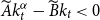 $\widetilde {A}k_{t}^{\alpha }-\widetilde {B}k_{t}\lt 0$
, this implies
 $ m_{t}=0$
. Therefore, after a finite number of iterations in which
 $ E_{t+1}=(1-b)E_{t}-\beta C_{t}$
, we would certainly have
 $m_{t}\gt 0$
, but this is not compatible with
 $m_{t}$
being definitely positive. Therefore, the dynamics either become non-admissible or oscillate between
 $m_{t}=0$
for a finite number of iterations and a single iteration with
 $m_{t}\gt 0$
.
If
 $\widetilde {B}\lt 0$
and
 $\widetilde {A}\gt 0$
, the next iteration is always feasible (with
 $m_{t}$
positive or zero).
If
 $\widetilde {B}\lt 0$
and
 $\widetilde {A}\lt 0$
, the next iteration is always feasible if
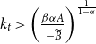 $k_{t}\gt \left ( \frac {\beta \alpha A}{{^{^{^{^{^{\!}}}}}}-\widetilde {B}}\right ) ^{ \frac {1}{1-\alpha }}$
. On the contrary, if
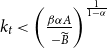 $k_{t}\lt \left ( \frac {\beta \alpha A }{{^{^{^{^{^{\!}}}}}}-\widetilde {B}}\right ) ^{\frac {1}{1-\alpha }}$
, the condition
 $ k_{t}\gt \left ( \frac {\widetilde {A}}{{^{^{^{^{^{\!}}}}}}\widetilde {B}}\right ) ^{\frac {1}{1-\alpha } }$
must hold.
To complete the study, we note that when
 $\beta A\alpha k_{t}^{\alpha }+ \widetilde {B}k_{t}\leq 0$
, it is possible to have an interior solution or a corner solution for
 $m_{t}$
. On the other hand, to have dynamics that, starting from
 $m_{t-1}\gt 0$
, define
 $m_{t}\gt 0$
– and therefore
 $k_{t+1}$
defined by map
 $T$
in the main text, the following conditions
 \begin{align*} \left \{ \begin{array}{c} \widetilde {A}k_{t}^{\alpha }-\widetilde {B}k_{t}\gt 0 \\ (\eta (1-\alpha )(1-\tau )\gamma +\beta \alpha )Ak_{t}^{\alpha }+\widetilde {B }k_{t}\gt 0 \end{array} \right .{\kern-.5pt}\! , \end{align*}
must hold. Therefore,
if
 $\widetilde {A}\gt 0$
and
 $\widetilde {B}\gt 0$
, then
 $k_{t}\lt \left ( \frac { \widetilde {A}}{{^{^{^{^{^{\!}}}}}}\widetilde {B}}\right ) ^{\frac {1}{1-\alpha }}$
must hold;
if
 $\widetilde {A}\gt 0$
and
 $\widetilde {B}\lt 0$
, then
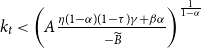 $k_{t}\lt \left ( A\frac {\eta (1-\alpha )(1-\tau )\gamma +\beta \alpha }{{^{^{^{^{^{\!}}}}}}-\widetilde {B}}\right ) ^{\frac {1}{ 1-\alpha }}$
must hold;
if
 $\widetilde {A}\lt 0$
and
 $\widetilde {B}\gt 0$
then interior solutions for
 $ m_{t}$
cannot exist;
if
 $\widetilde {A}\lt 0$
and
 $\widetilde {B}\lt 0$
, then
 $\left ( \frac {-\widetilde {A} }{{^{^{^{^{^{\!}}}}}}-\widetilde {B}}\right ) ^{\frac {1}{1-\alpha }}\lt k_{t}\lt \left ( A\frac {\eta (1-\alpha )(1-\tau )\gamma +\beta \alpha }{{^{^{^{^{^{\!}}}}}}-\widetilde {B}}\right ) ^{\frac {1}{ 1-\alpha }}$
must hold.
Appendix B
This appendix considers the problem of a social planner aiming to optimize social welfare given the optimal choices of consumers and firms. The problem can be formalized as follows:
 \begin{align*} & \max _{(K_{t},E_{t},H_{t},\tau _{t})}\sum \limits _{t=0}^{+\infty }\rho ^{t}[\!\ln (C_{t+1}^{\ast })+\eta \ln (E_{t+1})] \\ & s.t. \\ K_{t+1}& =w_{t}^{\ast }H_{t}(1-\tau _{t})-m_{t}^{\ast }, \\ E_{t+1}& =(1-b)E_{t}-\beta _{i}C_{t}^{\ast }+\gamma m_{t}^{\ast }, \\ H_{t+1}& =H_{t}(\tau _{t}w_{t}^{\ast }+z)^{\phi }, \\ C_{t}^{\ast }& =A\alpha K_{t}^{\alpha _{t}^{\ast }}H_{t}^{1-\alpha _{t}^{\ast }}+(1-\delta )K_{t}, \\ w_{t}^{\ast }& =(1-\alpha _{t}^{\ast })AK_{t}^{\alpha _{t}^{\ast }}H_{t}^{-\alpha _{t}^{\ast }}, \\ m_{t}^{\ast }& =\frac {AK_{t}^{\alpha _{t}^{\ast }}H_{t}^{1-\alpha _{t}^{\ast }}[(1-\alpha _{t}^{\ast })(1-\tau _{t})\gamma \eta +\beta _{t}]-(1-b)E_{t}+(1-\delta )K_{t}}{\gamma (1+\eta )}, \\ \alpha _{t}^{\ast }& =\underset {\alpha _{t}\in \left \{ \alpha _{L},\alpha _{H}\right \} }{\arg \max }\left ( A\alpha _{t}K_{t}^{\alpha _{t}-1}H_{t}^{1-\alpha _{t}}\right ) , \\ \beta _{t}& =\beta _{L}\text{ if }\alpha _{t}^{\ast }=\alpha _{L}\text{ and } \beta _{t}=\beta _{H}\text{ if }\alpha _{t}^{\ast }=\alpha _{H}, \\ & K_{0},\ E_{0},\ H_{0},\ C_{0}\ \text{given}, \end{align*}
where
 $\rho \gt 0$
is the inter-temporal discount factor of the planner. The necessary conditions for optimality can be derived from the Lagrangian function:
 \begin{align*} L& =\sum \limits _{t=0}^{+\infty }\rho ^{t+1}\left \{ \left ( \ln (C_{t+1}^{\ast })+\eta \ln ((1-b)E_{t}-\beta C_{t}^{\ast }+\gamma m_{t}^{\ast })\right ) +\ldots \right . \\ & \quad +\lambda _{t+1}^{1}\left [ w_{t}^{\ast }H_{t}(1-\tau _{t})-m_{t}^{\ast }-K_{t+1}\right ] +\ldots \\ & \quad +\lambda _{t+1}^{2}\left [ (1-b)E_{t}-\beta C_{t}^{\ast }+\gamma m_{t}^{\ast }-E_{t+1}\right ] +\ldots \\ & \quad +\left . \lambda _{t+1}^{3}\left [ H_{t}(\tau _{t}w_{t}^{\ast }+z)^{\phi }-H_{t+1}\right ] \right \} , \end{align*}
but given the complexity of the problem’s formulation, they are difficult to interpret. Indeed, to the best of our knowledge, no one has explicitly studied a similar issue in an OLG context like those considered in this work, with the exception of Yoshida (Reference Yoshida1998), who in a simpler context than ours, characterises the first-best solution chosen by a planner and compares it with the laissez-faire economy. More specifically, Yoshida (Reference Yoshida1998) analyses the role of a consumption tax to correct for the negative environmental externality of consumption and the positive externality of environmental good provision. A short-lived government (aiming to maximize welfare of the current generation) wants to set the optimal tax rate to internalize only the intra-generational externality and this tax rate is lower than the first-best tax rate. A long-lived government (aiming to maximize the discounted welfare of all current and future generations) can achieve the first-best optimum path by setting a consumption tax rate that internalizes both intra- and inter-generational externalities. This optimal tax rate is precisely equal to the first-best rate derived from the social planner’s problem. The main message of Yoshida (Reference Yoshida1998)’s findings is that the following. The laissez-faire economy can be stagnant, growing, or collapsing. A government’s ability to correct these outcomes via tax policy depends crucially on its time horizon. While a short-sighted government can improve upon the Nash equilibrium, only a government concerned with future generations can implement the first-best policy that fully corrects for all environmental externalities.
In our model, the presence of three types of capital (environmental, physical, and human) makes the implementation of the optimal policy even more intricate.