2. Methods: experimental set-up

The experimental apparatus is sketched in figure 1. Laboratory experiments were performed in a water channel 8.00 m in length, L _y = 0.40 m in width, with a water depth of H _w = 0.50 m, already employed for urban canyon studies (Garau et al. Reference Garau, Badas, Ferrari, Seoni and Querzoli2018). A constant flow rate was imposed by a closed loop, and water depth was tuned by means of a sharp-crested weir downstream of the channel. A 0.10 m-thick honeycomb acted as a flow straightener at the inlet of the channel. It was followed by irregularly distributed pebbles (≈5 mm in diameter) along 2 m of the bottom of the channel to promote the development of a fully turbulent boundary layer upstream of the array of panels (Badas et al. Reference Badas, Ferrari, Garau, Seoni and Querzoli2020). The model farm consisted of an array of 20 equidistant and transparent polycarbonate rectangular panels, 1.5 mm thick and L = 30.0 mm wide, spanning the whole channel width. To minimise undesired light diffusion, the panels were painted black except in the vicinity of the mid-section of the channel, where they were transparent, to allow the whole area around the panels to be illuminated. Furthermore, they were glued to steel shafts (≈2 mm in diameter), hinged at their lateral ends at a height h = 25 mm. Set screws allowed the panels’ pitch to be locked at the prescribed angle. We denote the streamwise and vertical directions by x and z, respectively, with their origin at the ground in the middle of the space between the two panels delimiting the investigated periodic unit. The uniform panel orientation was guaranteed via specific templates, removed after locking the screw before the experiment. With the flow from left to right, the panel tilt angle, α, is defined as positive when rotation is clockwise, and negative when rotation is counterclockwise. We considered two spacing distances d between the panels, yielding inter-panel aspect ratios of AR = d/L = 5/3 ≈ 1.67 and AR = 10/3 ≈ 3.33. The first mimics a classical photovoltaic farm with packed panels (dense configuration), whereas the second mimics an agrivoltaic farm with a larger distance to allow for agricultural activities (sparse configuration).

Figure 1.

(a) Horizontal incoming mean velocity profile along the centreline, in inner variables: experiments with uncertainty (red dots) and logarithmic fit in the region 100 < z ⁺ < 300 (black line). The uncertainty bar width is two standard deviations. (b) Sketch of a periodic unit of the canopy framed in grey with its geometrical parameters. (c) Water channel with elements of the experimental apparatus.

Figure 1 Long description

Panel A: A scatter plot depicts the horizontal incoming mean velocity profile along the centerline in inner variables. The x-axis represents U+ and ranges from 10 to 20. The y-axis represents z+ and ranges from 10^2 to 10^3. Red dots indicate experimental data with uncertainty bars representing two standard deviations, and a black line shows the logarithmic fit in the region 100 < z+ < 300. Panel B: A schematic diagram illustrates a periodic unit of the canopy framed in grey, showing its geometrical parameters. The diagram includes labels for height (Hc), distance (d), angle (α), height (h), and length (L). The wind direction is indicated by a blue arrow. Panel C: A diagram of a water channel with elements of the experimental apparatus. The flow direction is indicated by a blue arrow. The setup includes turbulence generators, panels, a honeycomb section, a laser sheet, a free-surface suppression optical plate, and a measurement window centered around the 17th panel. The channel dimensions are labeled, including a 2-meter section for turbulence generators, a 5-meter section for panels, and an 8-meter section for the measurement window. The sharp-crested weir has a height of 0.5 meters.

In the present geometry, the canopy height H _c = h + L/2 sin( $\alpha$ ) is approximately 30 mm. The logarithmic fit of the incoming boundary-layer profile in figure 1a was performed in inner variables, i.e., U ⁺ = ln(z ⁺ )/κ + B (with U ⁺ = U/u _* ,U the streamwise velocity, κ = 0.41, z ⁺ = z u _*/ν, and B an additive constant), at each streamwise location over the range 100 < z ⁺ < 300, i.e., where the log law is typically assumed to be valid. The analysis yields u _* = 11.4 ± 0.4 mm s⁻¹, where the uncertainty denotes the standard deviation across streamwise locations. The corresponding roughness length, evaluated through z ₀ = (ν/u _*) exp(−κB), is z ₀ = 20 × 10^-3 ± 5 × 10^-3 mm $,$ i.e., z ₀ ≈ 10⁻³ H _c , in line with previous studies (Badas et al. Reference Badas, Ferrari, Garau, Seoni and Querzoli2020). The difference between data and logarithmic fit remains within 2.5% within the whole investigated height range (z ⁺ < 1300). Furthermore, the ratios between canopy height and channel length scales H _c /H _w ≈ 0.06 and H _c /L _y ≈ 0.075 are comparable to previous water-channel studies of two-dimensional obstacle arrays, suggesting that blockage effects in the investigated region are limited. Based on figure 1a, the incoming inner boundary-layer thickness is approximately δ ≈ 0.1 m, so that H _c  ≈ 0.3δ. Therefore the canopy is fully embedded within the incoming boundary layer, and the measurement focus is on the roughness-sublayer region (Di Bernardino et al. Reference Di Bernardino, Monti, Leuzzi and Querzoli2015). These fluid dynamic and geometrical conditions are in line with other previous studies (Badas et al. Reference Badas, Ferrari, Garau, Seoni and Querzoli2020; Di Bernardino et al. Reference Di Bernardino, Monti, Leuzzi and Querzoli2015; Garau et al. Reference Garau, Badas, Ferrari, Seoni and Querzoli2018).

We exploited the geometrical symmetry of the system, analysing the flow in the vertical channel mid-plane (x–z) (Badas et al. Reference Badas, Ferrari, Garau, Seoni and Querzoli2020). Non-buoyant particles (pine pollen) dispersed in water were illuminated on the measuring plane by a 2 mm-thick light sheet, generated by a diode laser and projected from above through a transparent optically rectified glass carefully placed just at the water surface above the investigation region. The plate was 1.5 m long, equipped with a smooth leading edge and carefully held aligned with the free surface, so as not to generate disturbances in the subcritical flume either upstream or downstream. Consequently, in the measurement region, the depth was constant, and the flow above the canopy was not open channel. A high-speed camera (2240 × 1740 pixels in resolution), placed perpendicular to the interrogation area, recorded 330 frames per second on a SSD disk array without compression. Following previous water-channel studies of periodic two-dimensional obstacle arrays, the measurement region was located at the 17th periodic unit, allowing the boundary layer and the canopy-top shear layer to fully develop over the sixteen upstream panels, as observed in similar canopy flows, see e.g. Badas et al. (Reference Badas, Ferrari, Garau, Seoni and Querzoli2020). Images were analysed via a feature-tracking velocimetry technique. Seeding particles were identified via the Harris corner detection algorithm. Displacements between successive frames were computed by comparison of interrogation windows (17 × 17 pixels) and by minimising the dissimilarity measured by a Lorentzian estimator (Besalduch et al. Reference Besalduch, Badas, Ferrari and Querzoli2013). Particle velocities were obtained by dividing the displacements by the corresponding interframe time interval. Velocities were made non-dimensional with the average free-stream velocity, U ≈ 0.24 m s⁻¹, of each experiment. The Reynolds number based on the panel length, L, Re = UL/ν, is approximately 7,000 (ν = 10⁻⁶ m² s⁻¹ indicates the kinematic viscosity of the water). Conversely, using the incoming mean velocity at canopy height, U(H _c ), we obtain Re _Hc = UH _c /ν ≈ 7,000, while the friction Reynolds number is Re _τ = u _* H _c /ν ≈ 342. These values place the flow in a turbulent regime typically considered for experimental water-channel studies in urban-canopy flows, where Reynolds number effects have been reported to be small enough so that the main flow features are captured (Badas et al. Reference Badas, Ferrari, Garau, Seoni and Querzoli2020; Britter & Hanna Reference Britter and Hanna2003; Di Bernardino et al. Reference Di Bernardino, Monti, Leuzzi and Querzoli2015, Reference Di Bernardino, Monti, Leuzzi and Querzoli2020 a; Uehara et al. Reference Uehara, Wakamatsu and Ooka2003). Furthermore, Uehara et al. (Reference Uehara, Wakamatsu and Ooka2003) proposed also to verify that the region in which z ⁺ < 20 was limited, in our case, z < 1.8 mm ≈ 0.1 $H_{c}$ . We then evaluated the mean velocity field and the turbulence statistics by averaging instantaneous sparse velocity samples obtained from 10,000 velocity fields, corresponding to approximately 30 s, i.e. approximately 240 advective time scales (L/U), on a 97 × 131 regular grid. Convergence of second-order statistics was checked by comparing turbulent kinetic energy (TKE) and Reynolds-stress profiles obtained from progressively increasing subsets of the ensemble. The profiles were found to be stable for the full set of 10 000 fields, with residual statistical non-dimensional uncertainty below 10⁻³ in all of the cases.

3. Mean-flow general structure

Figure 2 shows the streamlines and magnitude of the mean velocity field for the dense array of panels (AR = 5/3). We begin with the positive incidence cases. At a small incidence (α = 20°, figure 2a), the velocity field shows the typical characteristics of the flow around a flat plate (Smith et al. Reference Smith, Pisetta and Viola2021). The streamlines follow the panel, with a small recirculation on the upper surface, close to the leading edge (denoted as a in figure 2). The flow is accelerated in the convergent space between the panel and the ground, reaching its highest velocity where the gap is the narrowest (so-called vena contracta). Downstream of it, the flow decelerates and deflects upwards to impinge on the lower surface of the following panel, close to the leading edge, as is typical of the flow around flat airfoils. Subsequently, an intense, continuous streamwise flow also develops below the panels. At the vena contracta, velocities comparable to the external flow are reached. At higher incidence angles (α = 40° and 55°, figures 2c and 2e), two additional vortical structures appear. The first, labelled b, develops at the trailing edge as the flow separates from the panel. The second, labelled c, is located downstream of the vena contracta, where the flow decelerates and is redirected upwards. This adverse-pressure-gradient region is strong enough to trigger separation from the ground. Above that structure, high-velocity fluid from the upper flow is redirected toward the lower surface of the downwind panel. The lower surface is therefore exposed to larger velocities compared with the upper surface, which may enhance advective heat exchange. The vortex a is still present and increases in size. In summary, at α = 20°, two intense continuous streams develop both above and below the panels. Conversely, at α = 40° and α = 55°, the inter-panel regions are dominated by recirculating structures, suggesting lower ventilation in the canopy layer.

Figure 2.

Dense case (AR = 5/3): streamlines of the mean velocity field overlaid with colour maps of the mean velocity magnitude, for (a, c, e) positive and (b, d, f) negative incidence.

We now focus on figures 2b, 2d and 2f, where the incidence is negative. Overall, low-velocity recirculations dominate close to the ground. Regardless of the tilt angle, the flow topologies are rather different from those in the positive incidence case. Specifically, two main vortical structures dominate: the first is a clockwise recirculating vortex (denoted as d) generated by the separation at the trailing edge of the panel, in the upper part of the canyon; the second vortex (denoted as e) is a counterclockwise-rotating recirculation generated by the counter-streamwise flow developing below the panels. As the incidence increases, the recirculating structure d grows and progressively invades the entire canyon, while the vortex e weakens accordingly (figures 2d and 2f). Flow structures described in figures 2b, 2d and 2f) are reminiscent of the skimming flow that develops in urban canyons. Specifically, for negative incidence angles, large portions of the ground surface are exposed to counter-streamwise flow, while canyons are dominated by recirculation structures, suggesting a weak contribution of the mean flow to the canopy layer ventilation. However, the case α = −55° shows the highest velocity near the ground and panel upper surface due to the increased strength of the vortex d, suggesting the persistence of flow asymmetry due to the incidence angle.

Figure 3 shows the sparse panel configuration case (AR = 10/3). Overall, compared with the dense configuration, higher velocities are observed within the canopy. For moderate positive incidence (α = 20° and α = 40°, figures 3a and 3c), the velocity field structures are similar to those observed in figure 2a. A continuous streamwise flow develops below the panels, which accelerates through the convergent gap below the panels and, again, impinges close to the leading edge of the downwind panel. However, the recirculation at the ground developing at α = 40° (c in figure 3c) is smaller and velocities through the panel–ground gaps are of the same order as the external flow. The same phenomenon is anticipated and enhanced at the largest positive incidence, resulting in a recirculation occupying all the space left by the vortices at the upper surface of the upwind panel. Irrespective of the tilt angle, the recirculation region covers the entire upper surface of the panels even for α = 40° and α = 55°, the separation occurs both at the leading and trailing edge, generating two counter-rotating vortices (figures 3c and 3e). This flow structure is reminiscent of the wake interference regime observed in urban canopies (Hunter et al. Reference Hunter, Watson and Johnson1990). For α < 0, similarly to the dense case, the flow within the canyon is dominated by a counterclockwise vortex (labelled as e) leeward of the panels and a clockwise vortex at the ground just upwind of the panels (labelled as d).

Figure 3.

Large distance case (AR = 10/3): streamlines of the mean velocity field overlaid with colour maps of the mean velocity magnitude, for (a, c, e) positive and (b, d, f) negative incidence.

The analysis of the structures dominating the velocity field is leveraged to draw insights into the contribution of the mean flow to heat-exchange and transport processes occurring between the photovoltaic canopy and the overlying external flow. Low incidence angles result in the formation of a continuous streamwise flow under the panels, periodically accelerating and decelerating at velocity magnitudes comparable to those of the external flow. For positive incidence angles, the flow accelerates through the narrow gap beneath the panel and then decelerates, producing pressure recovery and upward deflection toward the lower surface of the following panel. For negative incidence, by contrast, the lower panel surface is mainly reached by fluid recirculating within the canopy, leading to weaker direct impingement and reduced mean-flow exchange. For large positive incidence (α = 40° or α = 55°), the development of multiple recirculation bubbles induces strong vertical velocities that enhance fluid exchange across the canopy, thereby improving photovoltaic canopy ventilation and promoting the dispersion of scalars toward the outer flow that might otherwise be simply advected downstream near the ground. In contrast, large negative incidence angles (α = –40° or α = –55°) lead to large recirculation regions within the canopy, with a limited exchange with the external roughness layer, and a general structure reminiscent of the skimming-flow regime, associated with little exchange between the canopy and the overlying layer (Oke Reference Oke1988). This suggests a more intense advective mixing for positive than for negative incidence angles. Eventually, it is worth noting that the resulting mean velocity fields align with two-dimensional Reynolds Averaged Navier-Stokes (RANS) simulations of panel arrays at real scale (Ledda et al. Reference Ledda, Angius, Badas and Querzoli2024).

4. Mixing and transport through turbulent statistics and integral indices

We next present the mechanisms of advection by the mean flow, mixing and dispersion that result from the interaction between photovoltaic roughness and the atmospheric boundary layer. These are the key elements to be considered in the design of an agrivoltaic farm to optimise the microclimate for agricultural and energy production.

4.1. Turbulent kinetic energy

The in-plane TKE, measured in the centreline vertical plane of the water channel under consideration, is TKE = 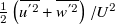$\frac{1}{2} \left(\overline{u^{'2}}+\overline{w^{'2}} \right)/U^{2}$ , where the overbar denotes the time average. The TKE plays a crucial role in dispersing scalars within and above the canopy. Figure 4 presents the TKE distributions for two large positive and negative incidence angles at both AR values. Notably, much higher TKE values within the canopy and roughness layers are observed when the incidence angle is positive. A closer look shows that, for positive incidence angles, relatively high TKE values are observed on the lower panel surfaces and in the decelerating flow downstream of the vena contracta. Conversely, for negative incidence, the skimming-like flow allows the penetration of relatively high TKE only in the downwind portion of the upper canyon interface, a region that linearly expands with the streamwise distance because of the developing instability of the shear layer.

Figure 4.

Streamlines of the mean velocity overlaid with colour maps of the non-dimensional TKE. Left column (a, c): dense distribution case and α = ±40°. Right column (b, d) sparse distribution case and α = ±55°. Spatial coordinates are made non-dimensional by the panel length, L.

The present results highlight the role played by the panels that interact with the incoming flow as flat airfoils actively deflecting the flow, rather than behaving as bluff bodies such as buildings or vegetation. Therefore, the canopy-top shear-layer dynamics is deeply affected by the incidence angle. For positive incidence angles, the interaction between the high-momentum outer flow and the low-momentum fluid from the canopy, ejected just upstream of the leading edge of the panel, promotes turbulence production and explains the elevated TKE observed in the overlying roughness sublayer and, in the sparse case, also within the canopy. The high-TKE regions observed in the sparse configuration downstream of the under-panel gap and near the lower panel surfaces are associated with flow upward deflection. For negative incidence angles, instead, the TKE maps depict a skimming-like regime dominated by large recirculation structures within the canopy. In this case, turbulence penetration is reduced, and high TKE remains mainly confined to the upper downwind portion of the canopy, with reduced interaction between canopy and outer flow.

4.2. Horizontally averaged vertical profiles

We now summarise the above results into vertical profiles by horizontally averaging the quantities over a periodic unit. Figures 5a and 5b report the vertical profiles of the non-dimensional average horizontal velocity, U _m , which give an indication of both the streamwise advection driven by the mean flow and how the panels affect the structure of the atmospheric boundary layer. For α = 20°, a significant positive horizontal average velocity is observed in the lower canopy layer (z < 0.5H _c ), and velocities attain values of approximately U _m ≅ 0.3 for 0.1H _c < z < 0.3H _c , independently of the panel distance. Nearly negligible positive velocities are observed for z < 0.2H _c , in the cases α = 40° and α = 55°. For negative incidence (α = −40°, −55°), the velocity is negative in the lower half of the canopy, suggesting a moderate upwind overall transport below the panels. However, at a height of approximately 0.7H _c , the average horizontal velocity becomes positive, with a logarithmic increase. This height marks the transition between the lower recirculating region and the overlying streamwise flow (Di Bernardino et al. Reference Di Bernardino, Monti, Leuzzi and Querzoli2020 a).

Figure 5.

Vertical profiles of the nondimensional horizontal velocity component horizontally averaged over the periodic unit, U _m , in the (a) dense and (b) sparse cases, and non-dimensional TKE for (c) dense and (d) sparse cases. Colour indicates the incidence angle according to the scale on the right.

Figure 5 Long description

The image contains four line graphs comparing vertical profiles of nondimensional horizontal velocity and turbulent kinetic energy in dense and sparse photovoltaic panel arrays. Panel A: A line graph shows the nondimensional horizontal velocity component (U_m) for a dense array. The x-axis represents U_m, ranging from -0.5 to 1, and the y-axis represents the normalized height (z/H_c), ranging from 0 to 2. Different colored lines indicate varying incidence angles. Panel B: A line graph shows the nondimensional horizontal velocity component (U_m) for a sparse array. The x-axis represents U_m, ranging from -0.5 to 1, and the y-axis represents the normalized height (z/H_c), ranging from 0 to 2. Different colored lines indicate varying incidence angles. Panel C: A line graph shows the nondimensional turbulent kinetic energy (TKE) for a dense array. The x-axis represents TKE, ranging from 0 to 0.4, and the y-axis represents the normalized height (z/H_c), ranging from 0 to 3. Different colored lines indicate varying incidence angles. Panel D: A line graph shows the nondimensional turbulent kinetic energy (TKE) for a sparse array. The x-axis represents TKE, ranging from 0 to 0.4, and the y-axis represents the normalized height (z/H_c), ranging from 0 to 3. Different colored lines indicate varying incidence angles. The color scale on the right indicates the incidence angle, ranging from -55 to 55.

Figures 5c and 5d show the non-dimensional TKE horizontally averaged over the periodic unit for the dense and sparse panel cases. A positive incidence yields significantly high turbulence values that strongly depend on the incidence itself, whilst negative incidence is associated with a much lower TKE and correspondingly lower dependence on α, in agreement with figure 4. Specifically, irrespective of the panel spacing, negative incidence cases are characterised by low TKE values, which are almost negligible for z < 0.7H _c . Conversely, positive α is associated with a more turbulent flow, with the TKE being maximum at z ≃ 0.8 H _c , where the interfacial shear layer develops. Similarly, in the dense case (figure 5c), a marked TKE peak occurs within the canopy at approximately z = 0.8H _c . This peak intensity diminishes markedly as the (positive) incidence increases. Increasing the distance (figure 5d) leads to very similar TKE values, although the turbulence propagates more above the canopy, in the roughness layer, for large and positive incidence. In these cases, reminiscent of the wake interference regime, the peak is no longer as marked as in the dense case.

In summary, the incidence has a notable effect on the TKE distribution across and above the canopy, not only on its spatial distribution, but also on its magnitude, due to the different interaction between the flow and the panels depending on the sign of the incidence. For negative incidence, the main flow above the canyon tends to skim over the canopy without deeply penetrating it, thus resulting in a dominant recirculating vortex confined within the canyon. Consequently, the interfacial velocity gradient is mitigated, preventing the development of a sharp shear layer. In this condition, the exchange between the canyon and the overlying flow is largely limited, consistently with the observed low TKE values. In contrast, for positive incidence, the recirculation vortices on the upper surface of the panels enhance the shear-layer intensity and the exchange between the near ground and the upper interface of the canopy and above the roughness layer, promoting the flow instability and increased turbulence.

Eventually, figure 6 shows the mean profiles of Reynolds stresses ( $\tau _{R}= -\overline{u'w'}/U^{2}$ ), which quantify the momentum transfer driven by turbulent fluctuations and, specifically, the vertical transport of horizontal momentum (Di Bernardino et al. Reference Di Bernardino, Monti, Leuzzi and Querzoli2020 b). The plots confirm the peculiar role played by the panels, which interact with the incoming flow more like flat airfoil profiles rather than bluff bodies, thereby modifying the structure of the roughness sublayer, Reynolds stresses’ magnitude and their vertical distribution, depending on the angle of incidence. There is a clear distinction between positive and negative incidence angles: with α > 0, the values of τ_R are consistently higher, compared with the α < 0 case, and are generally increasing with height up to z > 2H _c . The increase extends over the investigated region (which does not include the full outer boundary layer) in the case α = +20° both in the dense and sparse panel arrangement. In this framework, the turbulent momentum flux is not confined to the immediate canopy interface, as in urban canopies, but extends upward as coherent structures generated at the canopy top grow and interact with the overlying flow (Finnigan Reference Finnigan2000; Ghisalberti & Nepf Reference Ghisalberti and Nepf2002; Raupach et al. Reference Raupach, Finnigan and Brunei1996). In summary, the Reynolds-stress profiles complement the TKE analysis by showing that the enhanced turbulence in the positive incidence cases is associated with an effective vertical transport of streamwise momentum. Conversely, for negative incidence, the weaker canopy-top interaction and the dominance of in-canopy recirculation reduce both turbulence magnitude and momentum exchange.

Figure 6.

Vertical profiles of the non-dimensional Reynolds stress τ_R , horizontally averaged over the periodic unit for the (a) dense and (b) sparse cases and for varying incidence angle according to the colour scale.

This analysis suggests that the turbulent momentum transport is more intense when the incidence is positive, correlating with the highest values of TKE, in these conditions. Consequently, the overlying roughness layer experiences a greater degree of vertical mixing and momentum exchange as well as significantly larger TKE in the positive incidence configuration, which can have significant implications for processes such as scalar dispersion, canopy ventilation and energy distribution within the flow. These results are in line with the perspective of Glick et al. (Reference Glick, Ali, Bossuyt, Calaf and Cal2020 a), where a marked increase in the heat transfer coefficient was observed for large positive incidence. Furthermore, for very large negative incidence, flow structures are similar to those observed in idealised canyons with slender buildings (Badas et al. Reference Badas, Ferrari, Garau, Seoni and Querzoli2020). In the following, we investigate how the instantaneous flow affects ventilation and dispersion and relate it to the turbulent indices here described.

4.3. Canopy ventilation

To quantify ventilation, i.e., the vertical exchange of fluid across the depth of the photovoltaic canopy, we compute the exchange rate

\begin{equation*} \varphi _{e}\left(z\right)=\frac{1}{2Ud}\overline{\int _{\ell(z)}\left| w\left(x,z,t\right)\right| \mathrm{d}x}, \end{equation*}

where ℓ(z) is a horizontal line (of length d) across the periodic photovoltaic unit at height z, and the overbar, as usual, denotes time averaging. This non-dimensional index, widely used in urban and planetary boundary-layer studies, quantifies the volume of fluid exchanged across a horizontal surface per unit surface and time at a given height (Badas et al. Reference Badas, Ferrari, Garau and Querzoli2017, Reference Badas, Ferrari, Garau, Seoni and Querzoli2020; Garau et al. Reference Garau, Badas, Ferrari, Seoni and Querzoli2018). It should be noted that this is the most significant flux in the balance of the periodic photovoltaic unit, since the net flow along the horizontal direction is negligible, provided it is reasonable to assume a well-developed canopy layer since we focus on the 17th downwind periodic unit of the array (Badas et al. Reference Badas, Ferrari, Garau, Seoni and Querzoli2020). Therefore, the upwind flux equals the downwind flux. Evaluating the mass exchange at different heights z is relevant as it can be seen as a measure of the vertical transport within the canopy (Perret et al. Reference Perret, Blackman, Fernandes and Savory2017). Additionally, we computed the sole contribution of the mean flow (figure 7) to ventilation through $\varphi _{em}\left(z\right)=\frac{1}{2Ud}\int _{\ell\left(z\right)}| \overline{w}\left(x,z\right)| \mathrm{d}x$ (Garau et al. Reference Garau, Badas, Ferrari, Seoni and Querzoli2018). First, we analyse the values of $\varphi$ _e at z = H _c , which represents the overall net exchange between the canopy and the overlying roughness layer (table 1).

Table 1.

Exchange rate, $\varphi$ _e , and contribution of the mean flow, $\varphi$ _em , at the canopy top (z = H _c ), representing the net exchange between the canopy and outer flow

Table 1 Long description

A table comparing exchange rates and mean flow contributions at the canopy top for different angles. The table has 6 columns and 4 rows, including headers. The columns are labeled with angles: -55, -40, -20, +20, +40, and +55. The rows are labeled with different aspect ratios (AR) and variables: φe (Hc) for AR = 5/3, φe (Hc) for AR = 10/3, φem (Hc) for AR = 5/3, and φem (Hc) for AR = 10/3. Each cell contains a numerical value representing the exchange rate or mean flow contribution at the specified angle and aspect ratio. Row 1: φe (Hc) AR = 5/3, 0.0346, 0.0337, 0.0321, 0.0774, 0.0608, 0.0546. Row 2: φe (Hc) AR = 10/3, 0.0445, 0.0080, 0.0372, 0.0799, 0.0811, 0.0673. Row 3: φem (Hc) AR = 5/3, 0.0052, 0.0066, 0.0040, 0.0274, 0.0061, 0.0005. Row 4: φem (Hc) AR = 10/3, 0.0082, 0.0087, 0.0089, 0.0391, 0.0195, 0.0224.

Figure 7.

Streamlines of the mean velocity field overlaid with colour maps of the mean vertical velocity, for the dense case with α = +20° (a) and −20° (b).

In the dense panel configuration (AR = 5/3) and negative incidence, the exchange rate is low, and its value is $\varphi$ _e ≈ 0.03, regardless of the angle. Conversely, for positive incidence, $\varphi$ _e is higher, and decreases from approximately twice to one and a half times the exchange given by the negative incidence, as α increases. This difference agrees with the mean vertical velocity maps shown in figure 7 at $\alpha =\pm 20^{\circ }$ . For positive incidence (figure 7a), the flow exhibits an intense vertical motion across the canopy top, with large positive velocities spanning from the ground to the canopy top and extending into the overlying layer, in the inter-panel gaps. This structure, completely absent with negative α (figure 7b), indicates an active mean contribution to vertical exchange of momentum. In the sparse case (AR = 10/3), the exchange rates $\varphi$ _e (H _c ) are higher than in the dense configuration, except for the negative incidence angle α = –40°, which gives the lowest exchange rate among the investigated configurations. The highest value of the sparse case ( $\varphi$ _e ≈ 0.08) is attained at moderate positive angles (α = 20° and α = 40°), a value similar to that of the dense case. Figure 8 presents the vertical profiles of $\varphi$ _e and $\varphi$ _em as functions of z/H _c . In both cases, negative incidence angles lead to lower exchange rates compared with positive angles. Profiles of the exchange rates qualitatively vary both with incidence and AR: $\varphi$ _e is only weakly dependent on the incidence, when positive in the lower canopy layer (z < 0.6H _c ), although a slightly higher dependence is observed for the sparse configuration. The fluid exchange is higher with positive incidence, irrespective of the angle and AR. As concerns $\varphi$ _em , in the AR = 10/3 configuration, a large positive incidence promotes exchange between layers, whereas negative incidence yields profiles similar to those observed in urban canyons, characterised by a maximum at mid-height and a decay at the canopy top (Garau et al. Reference Garau, Badas, Ferrari, Seoni and Querzoli2018). In the dense case, all negative angles converge to very similar values at the top, in agreement with the skimming-flow characteristics. The difference between $\varphi$ _e and $\varphi$ _em increases for the sparse case, highlighting a higher contribution of turbulence to the exchange rate. Eventually, focusing again on $\varphi$ _e, in the dense case and negative angle, $\varphi$ _e shows an increasing trend, with higher values close to the canopy top. These trends are analogous to those observed in urban canyons (Garau et al. Reference Garau, Badas, Ferrari, Seoni and Querzoli2018).

Figure 8.

Vertical profiles of the exchange rate for the two distances and for varying incidence according to the colour scale on the right.

In summary, in the sparse case and for positive incidence, the periodic flow expansions between the panels and the ground generate high-momentum, continuous vertical turbulent transport throughout the canopy. The high TKE levels observed in these cases agree with the large differences between $\varphi$ _e and $\varphi$ _em , the signature of a primary role of turbulent fluctuations in the air exchange. Conversely, in the dense configuration and for large incidence (both positive and negative), a skimming flow with reduced mixing at the canopy top develops. These findings indicate that even small positive incidence angles can transform the canopy into an actively ventilated space, driven by continuous, panel-induced vertical turbulent transport. In contrast, a negative incidence establishes the weaker exchange between the canopy and the overlying boundary layer typical of skimming flows (Badas et al. Reference Badas, Ferrari, Garau, Seoni and Querzoli2020, Reference Badas, Garau and Querzoli2021). Even a modest positive incidence can substantially enhance exchange efficiency, promote moisture dispersion and improve thermal regulation in photovoltaic farms. It should be noted that $\varphi$ _e does not account for flow topology or trapping within recirculation regions, aspects that are accounted for in Section 5 by a Lagrangian analysis, specifically aimed at describing renewal and residence effects within the photovoltaic canopy.

5. Lagrangian dispersion of synthetic particles and turbulent dispersion coefficient

We perform a Lagrangian analysis of dispersion designed to describe the mixing of a passive tracer released close to the ground. To this end, for each experiment, we tracked 50 instantaneous releases of 10,000 synthetic particles, initially homogeneously distributed along a horizontal line at a height of z _s = h/4 and passively advected by integrating the instantaneous velocity field using a predictor–corrector algorithm. This choice is intended to be representative of a near-ground source of heat, moisture, pollen or other scalars, released by the soil or vegetation (Moretta et al. Reference Moretta, Moriondo, Rossi, Carvalho, Padovan, Dal Prà, Palchetti, Argenti, Staglianò, Balingit and Leolini2025; Suttie Reference Suttie2000). The region of interest is centred on a panel, with periodic boundary conditions imposed at the boundaries of the periodic unit. The particle and release number was verified to be high enough to attain statistical convergence. Similarly, to obtain statistically meaningful results, the simulation was advanced for 15,000 frames corresponding to 364 L/U (with L/U = 0.125 s), for each release. To this aim, the measured instantaneous velocity fields have been used cyclically in time during the integration. The time interval between the releases was heuristically set, after some preliminary tests, to 2.4 L/U to fully capture the sensitivity to initial conditions of the particle trajectories that characterise the turbulent flows, from a Lagrangian perspective. Figure 9 shows particles at non-dimensional times t ^* = 0, 2, 4, 6, with t ^* = t U/L at incidence angle α = ± 40° for both the investigated panel spacings.

Figure 9.

Synthetic particle (green dots) dispersion in the cases of incidence angles α = ±40° at non-dimensional times t ^*= 0, 2, 4, 6. Particle trajectories are obtained by integrating instantaneous velocity fields starting from a horizontal homogeneous distribution at z = 0.25h.

The differences in the dispersion, mainly between the cases with positive and negative angles, are apparent, and can be appreciated more in the Supplementary Videos 1–4. To quantify the exchanges between the photovoltaic canopy and the overlying boundary layer, we then compute the fraction of particles remaining beneath the panels (z < H _c ) as a function of time, averaged over all releases, N _b ^*(t ^*) (figure 10). For negative incidence angles and both panel spacings, this decay is monotonic. In contrast, large positive incidence cases exhibit non-monotonic behaviours, where an initial decay is followed by one or more reinjections of particles below the panels, highlighting the key role of large-scale coherent structures in the dispersion process. The characteristic time of this reinjection is larger (t ^* ≈ 175) for the dense configuration compared with the sparse configuration (t ^* ≈ 150). The sparse case also exhibits a narrower peak, a signature of a more definite characteristic time. Both the above-mentioned times are too long compared with the advective time across the periodic unit (1.67 L/U and 3.33 L/U, for the dense and sparse configurations, respectively) to be ascribed to the downward periodical deflection of the flow by the panels, also because the latter interpretation would contrast with the characteristic time decrease with AR.

Figure 10.

(a, b) Evolution of the average fraction of particles below the canopy as a function of non-dimensional time. The shaded areas span one standard deviation. (c) Non-dimensional half-life of N _b ^*(t ^*), T _h ^*, as a function of the incidence angle, α, for the dense and sparse spacings according to the legend.

From figures 10a and 10b, we compute the time taken for half of the particles to leave the canopy (i.e., the half-life of N _b ^*(t ^*)) rescaled by the advective time scale L/U, which will be denoted as T _h ^*. In the well-mixed box idealisation, T _h ^* is a proxy of the mean residence time of the particles within the canopy. Results are shown in figure 10c as a function of the incidence angle for the two panel spacings. In agreement with the previous results, negative incidence angles yield longer T _h ^*. The dependence on the sign of α is more intense in the dense spacing case, which gives the longest half-life for α < 0. In summary, a positive incidence substantially reduces particle residence times beneath the canopy, enhancing ventilation and mixing, while negative incidence cases trap particles for longer periods.

The dispersion from a source close to the ground is described by the statistics of the particle height as a function of time from the release. Specifically, we report the mean particle height, $\overline{z}$ (t*)/h, and its standard deviation σ _z (t ^*)/h (figure 11). The analysis is limited to t ^* = 15 to avoid biases due to particles exceeding the maximum investigated height. Subsequently, we describe only the initial stage of the dispersion, when the process is dominated by the small-scale turbulence within the canopy. Generally, the behaviour agrees with the above description, with the higher the increase in the average height, the higher the standard deviation (figure 11b). The highest and lowest σ _z curves are given by the dense spacing with α = ±20°. After an initial linear transient of faster growth due to Lagrangian correlation along particle trajectories, most of the σ _z curves present a square-root behaviour, in agreement with Taylor theory.

Figure 11.

Mean (a) and standard deviation (b) of synthetic particle height made non-dimensional by h, as functions of non-dimensional time. The colour indicates the incidence angle according to the colour scale on the right. Continuous lines: dense configurations (AR = 5/3); dashed lines: sparse configurations (AR = 10/3).

Fitting this interval of the non-dimensional standard deviation σ _z (t ^*)/h with the function $f(t^{\mathrm{*}})=at^{\mathrm{*}1/2}+b$ , (being b an arbitrary time shift that accounts for the initial, non-Gaussian, dispersion) allows the non-dimensional turbulent dispersion coefficient within the canopy (i.e., the inverse turbulent Péclet number) to be estimated as D _T /(LU) = $(a h / L)^2 / 2$ . Table 2 reports the inferred values for the investigated cases. For negative incidence, we observe moderate values that monotonically increase as the negative incidence angle increases, with a weak dependence on the distance. For positive incidence, the dispersion coefficients are much higher, with a greater dependence on the distance. In that case, high values are observed for α = 20°, regardless of the distance, whereas they decrease for α = 40° to increase again at α = 55°. For comparison, in water-channel urban-canopy experiments, Di Bernardino et al. (Reference Di Bernardino, Monti, Leuzzi and Querzoli2018) obtained D _T /(LU) ∼ 10^–3 – 10^–1. The present values, D _T /(LU)= 4 × 10⁻³ – 8 × 10⁻² fall within the same non-dimensional range, with negative incidence corresponding to the lower, skimming-like limit and positive incidence to the upper, shear-layer-dominated limit.

Table 2.

Non-dimensional turbulent dispersion coefficient for the investigated cases

Table 2 Long description

A table comparing non-dimensional turbulent dispersion coefficients for various cases. The table has 2 rows and 6 columns. The columns are labeled with incidence angles in degrees: -55, -40, -20, 20, 40, and 55. The rows are labeled with ‘Dense’ and ‘Sparse’. The values in the table are as follows: Row 1 (Dense): -55: 0.0147, -40: 0.0112, -20: 0.0040, 20: 0.0801, 40: 0.0285, 55: 0.0330. Row 2 (Sparse): -55: 0.0133, -40: 0.0146, -20: 0.0052, 20: 0.0569, 40: 0.0192, 55: 0.0579. The table shows that for negative incidence angles, the values are moderate and increase as the angle becomes more negative. For positive incidence angles, the values are higher and show a greater dependence on the distance, with notable peaks at 20 and 55 degrees.