1 Introduction
Streamwise-aligned riblets as a means of passively controlling wall-bounded turbulent flows have been well studied. Their ability to reduce the skin-friction drag has been reported by numerous researchers (Choi Reference Choi1989; Walsh Reference Walsh1990; Bechert et al.
Reference Bechert, Bruse, Hage, der Hoeven and Hoppe1997; Bechert, Bruse & Hage Reference Bechert, Bruse and Hage2000; García-Mayoral & Jiménez Reference García-Mayoral and Jiménez2011, to name a few), and the ribs’ near-wall stabilising mechanisms are discussed by Bechert & Bartenwerfer (Reference Bechert and Bartenwerfer1989), Choi (Reference Choi1989), Luchini, Manzo & Pozzi (Reference Luchini, Manzo and Pozzi1991). A bio-inspired riblet alignment was later introduced by Koeltzsch, Dinkelacker & Grundmann (Reference Koeltzsch, Dinkelacker and Grundmann2002), where the ribs are arranged in a converging and diverging (hereafter abbreviated as C–D) pattern. A converging texture is often observed upstream of sensory receptors on fast swimming sharks, and diverging texture is commonly observed around the lateral-line organs. This C–D pattern was tested by Koeltzsch et al. (Reference Koeltzsch, Dinkelacker and Grundmann2002) in a fully turbulent pipe flow, where one half of the inner surface of the pipe was covered with ribs which were yawed at
 $-45^{\circ }$
to the axial direction, and the other half at
 $+45^{\circ }$
. From their hot-wire experiments, Koeltzsch et al. (Reference Koeltzsch, Dinkelacker and Grundmann2002) observed a large azimuthal variation in the flow statistics. Above the line of flow convergence, the local mean axial velocity was lower, coupled with an increase in turbulence intensity. Above the region of flow divergence however, the opposite scenarios occurred. The C–D riblet pattern was later implemented in a turbulent boundary layer by Nugroho, Hutchins & Monty (Reference Nugroho, Hutchins and Monty2013), where they found higher/lower streamwise momentum deficit (hence a thicker/thinner local boundary layer) over the converging/diverging region respectively. They also characterised several parameters which affect the magnitude of this spanwise flow variation. From their mean-flow mapping using a hot-wire probe, they show that the rib’s yaw angle, viscous-scaled rib height and the flow development length over the C–D surface, affect the extent of boundary layer modification. A follow up study by Nugroho et al. (Reference Nugroho, Gnanamanickam, Monty and Hutchins2014) later indicated that this spanwise periodicity is also accompanied by time-average
 $\unicode[STIX]{x1D6FF}$
-scale streamwise roll modes. Relying on the spectrogram of streamwise velocity fluctuations, it was speculated that the C–D pattern might preferentially arrange the naturally occurring very-large-scale motions that are prevalent in wall-bounded turbulence (Kim & Adrian Reference Kim and Adrian1999; Adrian, Meinhart & Tomkins Reference Adrian, Meinhart and Tomkins2000b
; del Álamo et al.
Reference del Álamo, Jiménez, Zandonade and Moser2006; Hutchins & Marusic Reference Hutchins and Marusic2007; Monty et al.
Reference Monty, Stewart, Williams and Chong2007).
Time-average streamwise roll modes, commonly referred as the mean secondary flows, have also been identified in many recent studies over various surface roughness and topographies. To give a few examples, they are observed in open water channel flows over spanwise alternating smooth and rough bedforms (Wang & Cheng Reference Wang and Cheng2006), in turbulent boundary layers over spanwise-periodic obstacles aligned in the flow direction (Vanderwel & Ganapathisubramani Reference Vanderwel and Ganapathisubramani2015), over complex realistic roughness replicated from a damaged turbine blade (Barros & Christensen Reference Barros and Christensen2014) and also over spanwise alternating regions of wall drag (large-eddy simulation study by Willingham et al. Reference Willingham, Anderson, Christensen and Barros2014). It is a challenge to explain the physical mechanisms of how these time-average secondary flows arise. Anderson et al. (Reference Anderson, Barros, Christensen and Awasthi2015) analyse the aforementioned simulation results as well as the experiment over the complex turbine roughness, and attribute the occurrence of the time-average secondary flow to the uneven distribution of Reynolds stresses (following the turbulence kinetic energy balance approach of Hinze (Reference Hinze1967)).
The aim of the current study is to investigate how the turbulence structures behave under the deliberately triggered secondary flow over the C–D riblets, based on instantaneous particle image velocimetry (PIV) fields in the orthogonal cross-stream plane. The large field-of-view (FOV) measurement is designed to capture the full extent of the largest-scale modified structures. The single-point velocity statistics will also be discussed briefly to support and complement previous observations of Nugroho et al. (Reference Nugroho, Hutchins and Monty2013). The PIV snapshots offer a more detailed view of the instantaneous events that give rise to the time-average secondary flows previously observed over this herringbone pattern. Here the axis system
 $x$
,
 $y$
and
 $z$
refer to the streamwise, spanwise and wall-normal directions, with
 $u$
,
 $v$
and
 $w$
indicating the respective total velocity components.
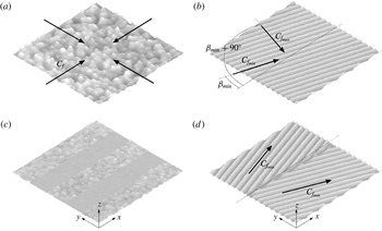
Comparison between surface topography with locally isotropic/anisotropic
 $C_{f}$
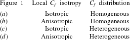
, in spanwise homogeneous/heterogeneous distribution. Refer to table 1 for the surface category.

Type of surface roughness categorised in figure 1.

2 Surface roughness
2.1 Surface roughness classification
There are endless rough surface topographies and arrangements that are present in nature and engineering. To date, the focus has been on the local roughness distributions and their effects on the flow. One convenient way to characterise roughness geometry is by its equivalent sand grain roughness height
 $k_{s}$
(Perry, Schofield & Joubert Reference Perry, Schofield and Joubert1969; Jiménez Reference Jiménez2004), which is effectively a measure of the roughness’ influence on the flow. Many physical attributes of the surface topography have been suggested to influence
 $k_{s}$
including (but not limited to) solidity, effective slope, skewness and average height (Acharya, Bornstein & Escudier Reference Acharya, Bornstein and Escudier1986; Napoli, Armenio & Marchis Reference Napoli, Armenio and Marchis2008; Flack & Schultz Reference Flack and Schultz2010; Chan et al.
Reference Chan, MacDonald, Chung, Hutchins and Ooi2015). Perhaps the most relevant roughness characterisation to this study is the ability of certain surfaces to induce large-scale secondary motions to the base flow, as is commonly observed over spanwise heterogeneous roughness (Hinze Reference Hinze1967; Wang & Cheng Reference Wang and Cheng2006; Vermaas, Uijttewaal & Hoitink Reference Vermaas, Uijttewaal and Hoitink2011; Mejia-Alvarez & Christensen Reference Mejia-Alvarez and Christensen2013; Barros & Christensen Reference Barros and Christensen2014; Willingham et al.
Reference Willingham, Anderson, Christensen and Barros2014; Vanderwel & Ganapathisubramani Reference Vanderwel and Ganapathisubramani2015). However, it is important to recognise that the surface that we are studying here differs to those listed above, in the sense that it exhibits both large-scale spanwise heterogeneity (roughness characteristics that vary as a function of
 $y$
) and directionality or anisotropy (a wall drag that depends on flow direction). To illustrate this distinction, figure 1 and the accompanying table show examples of surfaces under varying states of homogeneity and isotropy. To be clear, when we refer to heterogeneity or anisotropy, we refer to variations or directionality in roughness properties occurring over a wall-parallel length-scale that is
 $\gg k_{s}$
and some appreciable proportion of the layer thickness.
Figure 1(a) shows an example of an isotropic-homogeneous roughness which is represented by a sandpaper surface. A change in the instantaneous flow direction over this locally isotropic roughness causes no definite change in the skin-friction coefficient
 $C_{f}$
. In addition, the wall-drag distribution is homogeneous over this surface (i.e. is not a function of
 $x$
and
 $y$
location). To date, most engineering and meteorological surfaces are assumed to fall within this category, and indeed it is only for this roughness category that current tools permit full-scale predictions. This is usually obtained via the Moody chart for fully developed pipe flow (Moody Reference Moody1944; Shockling, Allen & Smits Reference Shockling, Allen and Smits2006) or developments for the zero-pressure-gradient flat plate turbulent boundary layer (Prandtl & Schlichting Reference Prandtl and Schlichting1955; Granville Reference Granville1958). Figure 1(b) displays an example of an anisotropic (directional)-homogeneous roughness which is represented by a standard riblets profile. As illustrated by this figure, a different instantaneous flow direction
 $\unicode[STIX]{x1D6FD}$
will yield a different value of
 $C_{f}$
. The minimum
 $C_{f}$
over the riblets will be obtained where the local flow direction is parallel with the grooves, and it will increase systematically with the yaw angle, to reach a maximum value when the motion is perpendicular to the grooves. The minimum/maximum resistance was examined by Luchini et al. (Reference Luchini, Manzo and Pozzi1991) using Stokes flow analysis, where they show the deeper/shallower protrusion heights for flow parallel/across the grooves. The anisotropy in skin-friction coefficient was also demonstrated by Walsh (Reference Walsh1990) who studied the dependence of riblets drag reduction with yaw angle. Similar to figure 1(a), the wall-drag distribution for this grooved surface is homogeneous though for a given flow direction. Transverse bars studied by Volino, Schultz & Flack (Reference Volino, Schultz and Flack2009), honed pipes investigated by Shockling et al. (Reference Shockling, Allen and Smits2006) or even wind over the ocean waves will also fit within this category.
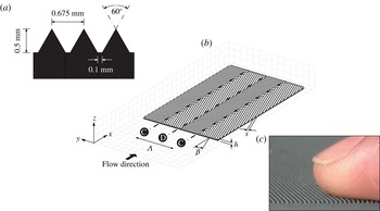
(a) Ribs cross-section. (b) Schematic drawing of the C–D riblets, showing several key parameters. (c) Picture of the actual riblet grooves.

Figure 1(c) gives an example of a surface with spanwise heterogeneity. The roughness is arranged in spanwise-alternating strips of varying roughness height. For flow in the
 $x$
direction, this surface is known to give rise to secondary flows centred about the step change of the wall drag (Hinze Reference Hinze1967; Wang & Cheng Reference Wang and Cheng2006; Willingham et al.
Reference Willingham, Anderson, Christensen and Barros2014). Note that although this surface has a degree of directionality (in the sense that it will perform quite differently when the flow is in the
 $y$
direction, hence it becomes a streamwise heterogeneous roughness), the individual roughness patches are locally isotropic. This is because the surface shown in figure 1(c) is comprised of sandpaper-type roughness. Therefore, we classify this surface as isotropic heterogeneous. Rivet rows on an aircraft fuselage that are commonly streamwise-aligned, spanwise-alternating river bedforms such as those studied by Wang & Cheng (Reference Wang and Cheng2006), and even the edges of forests under the atmospheric surface layer are examples of this surface type. Note that this isotropic-heterogeneous arrangement can also be formed in a more irregular manner than the example given in figure 1(c). This is demonstrated by the turbine blade roughness studied by Barros & Christensen (Reference Barros and Christensen2014) that produces distinct mean streamwise vortices above the surface, which are attributed to the large-scale (spanwise) topography variation that is present within the roughness complexity. Finally, figure 1(d) shows an anisotropic surface that also has a large-scale heterogeneity in the form of a spanwise-varying directional roughness. This surface closely resembles the pattern surrounding the sharks’ lateral-line organ (Koeltzsch et al.
Reference Koeltzsch, Dinkelacker and Grundmann2002) and also that found on the feathers of birds (Chen et al.
Reference Chen, Rao, Shang, Zhang and Hagiwara2014). Note that the minimum-
 $C_{f}$
vectors drawn represent the local direction of least resistance on this anisotropic surface. However, the study of Nugroho et al. (Reference Nugroho, Hutchins and Monty2013) over a similar pattern indicates that the mean streamwise wall drag is a complex function of spanwise location
 $y$
. Furthermore, large-scale secondary motion following a highly modified boundary layer is observed. In this paper we will further investigate how this anisotropic-heterogeneous surface produces such profound modifications to the turbulent boundary layer, despite having a small
 $k/\unicode[STIX]{x1D6FF}$
.
2.2 Converging–diverging riblets
The directional-heterogeneous roughness under study is a converging–diverging riblet arrangement similar to that originally fabricated and studied by Nugroho et al. (Reference Nugroho, Hutchins and Monty2013). It consists of a repeating pattern of alternating converging and diverging grooves arranged in a ‘herringbone-type’ pattern. Figure 2 is a schematic drawing of the riblet surface defining several key parameters. The height of each rib
 $h=0.5$
mm and the spacing
 $s=0.68$
mm, giving
 $h^{+}=hU_{\unicode[STIX]{x1D70F}s}/\unicode[STIX]{x1D708}\approx 18$
and
 $s^{+}=sU_{\unicode[STIX]{x1D70F}s}/\unicode[STIX]{x1D708}\approx 24$
(where
 $U_{\unicode[STIX]{x1D70F}s}$
is the smooth-wall friction velocity at the same inflow condition). At the present streamwise location, the rib height yields a blockage ratio of
 $h/\unicode[STIX]{x1D6FF}_{s}\approx 0.005$
(where
 $\unicode[STIX]{x1D6FF}_{s}$
is the smooth-wall boundary layer thickness). As shown in figure 2(a), the cross-section of the ribs represents a trapezoidal profile. This shape is the consequence of the 0.1 mm flat-chamfered tip of the
 $60^{\circ }$
cutter that was used to groove the surface. The ribs are yawed at an angle
 $\unicode[STIX]{x1D6FD}=\pm 20^{\circ }$
from the main flow direction to create regions of convergence and divergence. The width of each converging/diverging region is 73.75 mm, giving a repeating C–D wavelength of
 $\unicode[STIX]{x1D6EC}=147.5$
mm (or
 $\unicode[STIX]{x1D6EC}/\unicode[STIX]{x1D6FF}_{s}\approx 1.5$
). Note that the schematic drawing of figure 2(b) is not drawn to scale, where in reality one complete C–D wavelength
 $\unicode[STIX]{x1D6EC}$
consists of more than 200 yawed ribs. Figure 2(c) gives a sense of the actual rib dimensions.
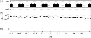
Comparison of the spanwise-profile surface topographies (about their mean elevation height) averaged over
 $\unicode[STIX]{x1D6FF}$
-long streamwise fetch, between the study of (a) Vanderwel & Ganapathisubramani (Reference Vanderwel and Ganapathisubramani2015), (b) Barros & Christensen (Reference Barros and Christensen2014) and (c) current study.

2.3 Does spanwise variation of wall drag cause the boundary layer modification over the converging–diverging riblets?
As previously discussed, a spanwise
 $C_{f}$
heterogeneity has been shown to give rise to secondary motions in the boundary layer. A recent paper by Anderson et al. (Reference Anderson, Barros, Christensen and Awasthi2015) addresses the qualitative flow similarity between the simulation by Willingham et al. (Reference Willingham, Anderson, Christensen and Barros2014) and the flow observed over the surface of Barros & Christensen (Reference Barros and Christensen2014). In all cases, they suggest that the wall-drag variation gives rise to the generation of the observed secondary flows, by creating an imbalance in the Reynolds stress distribution. A study by Vanderwel & Ganapathisubramani (Reference Vanderwel and Ganapathisubramani2015) also concludes that large-scale variation in surface elevation, which translates to varying aerodynamic wall drag, is able to produce a mean secondary flow (although it is noted that their mean secondary flows turn in an opposite sense to those listed above, with common flow up over the elevated regions). Over the C–D riblets studied here, spanwise variations of wall drag are also observed accompanying a highly modified boundary layer (see Nugroho et al.
Reference Nugroho, Hutchins and Monty2013). However, it is wise to be cautious in aligning the C–D riblet surface to the spanwise heterogeneous roughness listed above. Figure 3 puts this issue into perspective. It compares the spanwise surface profiles of (a) Vanderwel & Ganapathisubramani (Reference Vanderwel and Ganapathisubramani2015), (b) Barros & Christensen (Reference Barros and Christensen2014) and (c) the current study, averaged over a
 $\unicode[STIX]{x1D6FF}$
-long streamwise fetch. This streamwise averaging of surface topography was previously used by Barros & Christensen (Reference Barros and Christensen2014) to provide a qualitative representation of the imposed aerodynamic drag. In other words, the wall drag is higher when the profile is protruding, and is lower when the profile is recessed. Looking at figure 3(a,b), we can clearly see the variation in the surface height characterised as a spanwise heterogeneous surface. Over the C–D riblets however, there is no variation in the elevation over this streamwise-averaged profile, or
 $h\neq f(y)$
. Even if we do not streamwise average the C–D riblet topography, the cross-sectional profile will simply look like a regular rib (e.g. sawtooth/blade/trapezoidal) texture. The only thing that varies over the spanwise wavelength of the C–D pattern is the direction of the minimum/maximum flow resistance (Luchini et al.
Reference Luchini, Manzo and Pozzi1991). Hence, it would appear that the anisotropy or directionality in the C–D riblets may play a key role. Therefore, we should remain open to the possibility that different driving mechanisms might be responsible for generating the mean secondary flow in the C–D riblet case.
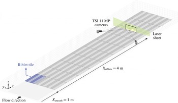
Schematic drawing of the stereoscopic PIV set-up, showing the surface configuration, laser sheet direction and camera arrangement.

3 Stereoscopic PIV experiments
The cross-stream plane stereoscopic PIV (sPIV) experiments are conducted in an open return suction-type wind tunnel at the University of Illinois at Urbana-Champaign. The wind tunnel has a working section of
 $6\times 0.91\times 0.46$
m. The characteristics of this tunnel have been documented in many past studies (Adrian et al.
Reference Adrian, Meinhart and Tomkins2000b
; Tomkins & Adrian Reference Tomkins and Adrian2003; Wu & Christensen Reference Wu and Christensen2010). Both the riblets and smooth-wall base-case experiments are conducted at a streamwise location of
 $x=5$
m at nominal free-stream velocity of
 $17.0~\text{ms}^{-1}$
. Both cases are performed under zero-pressure-gradient conditions. Figure 4 presents a schematic drawing of the sPIV set-up. For the riblet measurement, the boundary layer is first developed over a smooth wall for 1 m, then transitioned (with the crest of the riblets levels with the upstream smooth wall) and developed over the C–D riblets for 4 m. The C–D riblets were manufactured as a set of textured tiles made from polyurethane cast, with each tile having the dimension of
 $515\times 300$
mm. The readers are referred to Nugroho et al. (Reference Nugroho, Hutchins and Monty2013) for full details of the manufacturing technique. Additionally, the riblet surface is dyed black at the measurement location using polymeric colourant to reduce background reflection in the PIV images. A total of 30 riblet tiles are used to cover the floor of the wind tunnel working section, covering the entire spanwise width with three tiles, equivalent to six complete C–D wavelengths
 $\unicode[STIX]{x1D6EC}$
.
The flow is seeded with
 $1~\unicode[STIX]{x03BC}\text{m}$
olive oil droplets generated using 15 Laskin nozzle arrays, and illuminated with a 2 mm thick laser sheet generated by a dual-cavity 190 mJ per pulse Nd:YAG laser (Quantel) and a series of cylindrical lenses. The laser sheet enters the plane of interest from the side of the tunnel, which further minimises the frontal light reflection issuing from the riblet surface. The imaging system is two TSI 11MP cameras (
 $4000\times 2672$
pixels, 12-bit frame-straddled CCD) equipped with Sigma 180 mm macro lenses. The cameras view the cross-flow plane through optical-grade glass side walls at an upstream angle of
 $\pm 45^{\circ }$
from the streamwise direction. Uniform image focus is obtained across the entire FOV by satisfying the Scheimpflug condition. To observe the full extent of the largest-scale modified structures, a wide FOV in spanwise-wall-normal domain of
 $3.1\times 1.5\unicode[STIX]{x1D6FF}_{s}$
is captured, which spans approximately two complete C–D wavelengths. The stereoscopic calibration images are taken using a single-plane target (covering
 $2.8\times 1.5\unicode[STIX]{x1D6FF}_{s}$
) taken at five
 $x$
-locations with
 $250~\unicode[STIX]{x03BC}\text{m}$
separation. The mapping functions from the two-dimensional image space to the three-dimensional real space are computed using a least-squares polynomial with cubic dependence in the in-plane directions and linear in the out-of-plane direction. The derivatives of these mapping functions are used to reconstruct the three velocity components from the particle pixel displacements (which are computed in the warped image) based on the method proposed by Soloff, Adrian & Liu (Reference Soloff, Adrian and Liu1997). The pixel displacements are processed using an in-house PIV package, where the details of the processing algorithm are available in de Silva et al. (Reference de Silva, Gnanamanickam, Atkinson, Buchmann, Hutchins, Soria and Marusic2014). A final interrogation window size of
 $16\times 16$
pixel with 50 % overlap is employed. Since the velocity vectors are computed with a fixed interrogation window size throughout the entire image, the variation in the camera magnification due to perspective view results in the gradation of the spatial resolution, with the range of
 $93~\unicode[STIX]{x03BC}\text{m}~\text{pixel}^{-1}$
 $\pm 15\,\%$
in spanwise direction and
 $66~\unicode[STIX]{x03BC}\text{m}~\text{pixel}^{-1}$
 $\pm 10\,\%$
in wall-normal direction. Together with the laser-sheet thickness, these values yield a mean (viscous-scaled) interrogation spot size of
 $\unicode[STIX]{x0394}x^{+}\times \unicode[STIX]{x0394}y^{+}\times \unicode[STIX]{x0394}z^{+}=77\times 57\times 40$
for the smooth-wall base-case flow. Seven thousand three-component instantaneous velocity realisations are taken for the riblets case and 2500 for the smooth-wall case. An acquisition rate of 0.5 Hz is employed to ensure statistical independence, which is equivalent to approximately 350 boundary layer turn over times between consecutive snapshots.
To assess the quality of the experiments, a smooth-wall boundary layer measurement at lower Reynolds number of
 $Re_{\unicode[STIX]{x1D70F}}=2560$
(at the same streamwise location, with lower free-stream velocity of
 $U_{\infty }=10.9~\text{m}~\text{s}^{-1}$
) is also performed. This dataset allows a direct comparison to the existing boundary layer simulation of Eitel-Amor, Örlü & Schlatter (Reference Eitel-Amor, Örlü and Schlatter2014) at comparable Reynolds number of
 $Re_{\unicode[STIX]{x1D70F}}=2479$
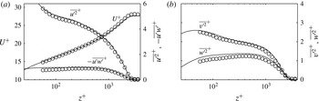
. Figure 5(a) shows the viscous-scaled mean streamwise velocity profile for the validation case. For clarity of presentation, the data points are down sampled to 30 wall-normal locations spaced logarithmically. A good collapse with the reference profile of Eitel-Amor et al. (Reference Eitel-Amor, Örlü and Schlatter2014) is clearly evident throughout the boundary layer. Figure 5(a,b) also presents the Reynolds stress profiles. Note that these second-order statistics have been corrected using a method proposed by Lee et al. (Reference Lee, Monty and Hutchins2016), to account for the spatial attenuation due to volume averaging inherent in PIV interrogation. This method essentially approximates the reduction in turbulence intensity profiles due to small-scale unresolved energy, simply given the finite interrogation volume size in viscous units. Despite the slight underestimation that remains in these fluctuation statistics, which may result from the spatial-resolution variation across the wide FOV, the facility and measurement system clearly yield the expected velocity statistics at this moderate Reynolds number.
Validation of sPIV statistics performed on the smooth wall at
 $Re_{\unicode[STIX]{x1D70F}}=2560$
. The second-order statistics are corrected using the method proposed by Lee et al. (Reference Lee, Monty and Hutchins2016) to account for the spatial attenuation due to finite PIV interrogation volume. Solid lines are reference statistics taken from simulation data of Eitel-Amor et al. (Reference Eitel-Amor, Örlü and Schlatter2014) at
 $Re_{\unicode[STIX]{x1D70F}}=2479$
.

Experimental parameters of the current sPIV experiments.

The experimental conditions as well as the PIV parameters are summarised in table 2. Note that for the C–D riblets case, since parameters such as
 $\unicode[STIX]{x1D6FF}$
and
 $\unicode[STIX]{x1D703}$
(hence
 $Re_{\unicode[STIX]{x1D703}}$
) are functions of spanwise location
 $y$
, the values presented in the table correspond to the spanwise-averaged value over one complete C–D wavelength
 $\langle \cdot \rangle _{\unicode[STIX]{x1D6EC}}$
. Here
 $\unicode[STIX]{x1D6FF}$
or
 $\unicode[STIX]{x1D6FF}(y)$
corresponds to the wall distance where the mean streamwise velocity reaches 99 % of the free-stream velocity. To highlight the physical modifications caused by the C–D riblets with respect to the smooth-wall base case, the ordinate of the velocity maps are normalised by the smooth-wall boundary layer thickness
 $\unicode[STIX]{x1D6FF}_{s}$
throughout this paper. The abscissa however, are normalised by the C–D wavelength
 $\unicode[STIX]{x1D6EC}$
while maintaining the physical aspect ratio. Here the diverging region is located at
 $y/\unicode[STIX]{x1D6EC}=0$
and converging region at
 $y/\unicode[STIX]{x1D6EC}=\pm 0.5$
(indicated by the


 $U_{\infty }$
. The flow direction in all the velocity maps presented is out of the page.
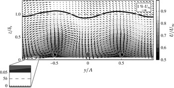
Contours of time-average streamwise velocity normalised by the free-stream velocity
 $U/U_{\infty }$
over the C–D riblets. The time-average in-plane velocity vectors
 $V$
and
 $W$
are superimposed. Solid line: local boundary layer thickness
 $\unicode[STIX]{x1D6FF}$
; dashed line: spanwise-averaged boundary layer thickness
 $\langle \unicode[STIX]{x1D6FF}\rangle _{\unicode[STIX]{x1D6EC}}$
. Inset highlights the rib height.

4 Velocity statistics and decomposition
4.1 Mean velocity field
Figure 6 shows contours of time (ensemble)-averaged streamwise velocity over the C–D riblets. Thick black contour line indicates the local boundary layer thickness
 $\unicode[STIX]{x1D6FF}(y)$
, and its spanwise-averaged value
 $\langle \unicode[STIX]{x1D6FF}\rangle _{\unicode[STIX]{x1D6EC}}$
is shown by the dashed line. Despite having groove heights of
 $h/\unicode[STIX]{x1D6FF}_{s}\approx 0.005$
as indicated by the inset, pronounced spanwise periodicity induced by the C–D pattern is clearly displayed in figure 6. The mean streamwise velocity is much lower near the converging region compared to the diverging at a given wall height. This variation in momentum defect extends up to the edge of the boundary layer resulting in a periodicity in the local
 $\unicode[STIX]{x1D6FF}$
, which is approximately
 $\pm 8\,\%$
of its spanwise-averaged value
 $\langle \unicode[STIX]{x1D6FF}\rangle _{\unicode[STIX]{x1D6EC}}$
. In some sense, this observation challenges the classical-roughness assumption which states that the roughness height needs to be at least of order
 $h/\unicode[STIX]{x1D6FF}\approx 1/40$
before its influence extends across the entire layer (Jiménez Reference Jiménez2004). However, it is important to recognise that the present surface exhibits anisotropy as well as spanwise
 $C_{f}$
heterogeneity. Spanwise heterogeneity in roughness height (figure 1
c) could also cause a similar scenario. In both cases, the wavelength of the heterogeneity seems to play a strong role in how far the three-dimensionality observed in the flow extends from the wall (see for example coarse- and fine-spaced results from Vanderwel & Ganapathisubramani Reference Vanderwel and Ganapathisubramani2015).
Similar mean streamwise velocity behaviour was previously shown by Nugroho et al. (Reference Nugroho, Hutchins and Monty2013) from the hot-wire flow mapping over the same type of riblets. They also attempted to approximate the wall drag over the line of convergence and divergence using the local velocity profiles. From both the modified-Clauser (Perry & Li Reference Perry and Li1990) as well as the momentum-integral method (Anders Reference Anders1990), they found that the converging pattern increases the wall drag (with respect to the smooth-wall comparison) whilst the diverging pattern reduces the drag. In this experiment, we found a similar wall-drag behaviour from three different estimation methods, namely modified-Clauser, momentum-integral and the total-shear-stress method (Flack, Schultz & Shapiro Reference Flack, Schultz and Shapiro2005). From these methods we tentatively estimate the drag increase over the converging region to be
 ${\sim}30\,\%$
and the drag decrease over the diverging to be
 ${\sim}20\,\%$
. Furthermore, recent pipe flow experiments by Chen et al. (Reference Chen, Rao, Shang, Zhang and Hagiwara2014) obtained significant total drag reductions over similar herringbone riblets (based on the changes in the pressure gradient), by replacing the converging regions with strips of smooth surface. This strategy works perhaps by negating the drag increase induced by the converging region, while still exploiting the drag reducing property of diverging riblet pattern. Therefore, in the absence of a direct wall-drag measure, we label the converging/diverging region as the region of higher/lower wall drag respectively, based on the aforementioned approximation techniques and consistent with the results of Chen et al. (Reference Chen, Rao, Shang, Zhang and Hagiwara2014).
The accompanying time-averaged in-plane velocity vectors
 $V$
and
 $W$
are also visualised in figure 6. The plot shows the existence of
 $\unicode[STIX]{x1D6FF}$
-filling counter-rotating roll modes in the mean field centred at
 $z/\unicode[STIX]{x1D6FF}_{s}\approx 0.3$
. The maximum mean vertical motion captured within this field of view is
 $W\approx 1.5\,\%$
of
 $U_{\infty }$
. The vectors also confirm that the mean common flow up occurs above the converging (higher wall-drag) region and mean common flow down occurs above the diverging (lower wall-drag) region. Periodic mean secondary flows are also observed over spanwise heterogeneous roughness tested by Wang & Cheng (Reference Wang and Cheng2006) and in simulation results analysed by Anderson et al. (Reference Anderson, Barros, Christensen and Awasthi2015). Interestingly, the sign of their streamwise vortices is the opposite of the one shown in the present study. They observed a mean common flow down over the higher drag region. It was noted by Hinze (Reference Hinze1973) however, that the rotational direction over this type of heterogeneous drag/roughness patches are not imperative. Depending on the roughness configuration, either common flow up or down can occur over the rougher patch. For the case of secondary flow observed by Vanderwel & Ganapathisubramani (Reference Vanderwel and Ganapathisubramani2015), the rotational sense seems to be similar to the current study (upward motion over the higher drag region). However, the results of Vanderwel & Ganapathisubramani (Reference Vanderwel and Ganapathisubramani2015) could be viewed more as spanwise changes in surface elevation rather than heterogeneous roughness. All these differences suggest that different driving mechanisms might be responsible for generating the mean secondary flow in each case. The orientation of the currently observed mean roll modes can be determined from a consideration of the direct influence of the ribs to the shear flow above them. The yawed riblets impose lesser/greater flow resistance in the direction parallel/misaligned to the grooves (Luchini et al.
Reference Luchini, Manzo and Pozzi1991), or alternatively, modify the forward mobility tensor as proposed by Kamrin, Bazant & Stone (Reference Kamrin, Bazant and Stone2010).
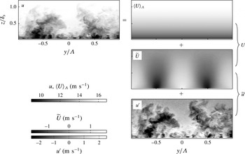
Example of total streamwise velocity field
 $u$
over the C–D riblets, triply decomposed into the global mean
 $\langle U\rangle _{\unicode[STIX]{x1D6EC}}$
, non-convecting spatial variation
 $\widetilde{U}$
and temporal/convecting fluctuation
 $u^{\prime }$
.

4.2 Velocity decomposition
Due to the spanwise periodicity present in the boundary layer, there is an opportunity to apply a triple decomposition to the velocity results. The total velocity in the cross-stream plane can be decomposed into,
 $$\begin{eqnarray}\displaystyle u_{i}(y,z,t) & = & \displaystyle U_{i}(y,z)+u_{i}^{\prime }(y,z,t)\end{eqnarray}$$
 $$\begin{eqnarray}\displaystyle & = & \displaystyle \langle U_{i}\rangle _{\unicode[STIX]{x1D6EC}}(z)+\widetilde{U}_{i}(y,z)+u_{i}^{\prime }(y,z,t)\end{eqnarray}$$
 $$\begin{eqnarray}\displaystyle & = & \displaystyle \langle U_{i}\rangle _{\unicode[STIX]{x1D6EC}}(z)+\widetilde{u}_{i}^{\prime }(y,z,t).\end{eqnarray}$$
 $u_{i}$
can be temporally/Reynolds decomposed into
 $U_{i}$
, which is the time-averaged mean velocity (also known as the local mean) and
 $u_{i}^{\prime }$
which is the turbulence (convecting) fluctuations about the time-averaged values. For the present surface,
 $U_{i}$
will be a function of
 $y$
and
 $z$
, reflecting the spanwise variation observed in figure 6.
 $\langle U_{i}\rangle _{\unicode[STIX]{x1D6EC}}$
is the spatially and temporally averaged mean velocity (also known as the global mean) taken by averaging
 $U_{i}$
over one complete C–D wavelength.
 $\widetilde{U}_{i}=U_{i}-\langle U_{i}\rangle _{\unicode[STIX]{x1D6EC}}$
is the spanwise variation of the time-averaged velocity. This term represents the spatial time-invariant variation of the flow, due to the more frequent occurrence of lower-/higher-speed fluid over the converging/diverging part of the riblets respectively. The non-zero values of this term add dispersive stress components
 $\langle \widetilde{U}_{i}\widetilde{U}_{i}\rangle _{\unicode[STIX]{x1D6EC}}$
to the stress tensor, which represent the additional transport of momentum by spatial flow variation in the spanwise direction (Coceal et al.
Reference Coceal, Thomas, Castro and Belcher2006). From (4.1c
),
 $\widetilde{u}^{\prime }$
is the combination of the non-convecting spatial variation
 $\widetilde{U}$
and the convecting turbulence fluctuation
 $u^{\prime }$
. Therefore, under this spatio-temporal decomposition, the converging region will most likely have negative
 $\widetilde{u}^{\prime }$
values close to the surface where the amplitude of the alternating positive/negative
 $\widetilde{U}$
is most pronounced.
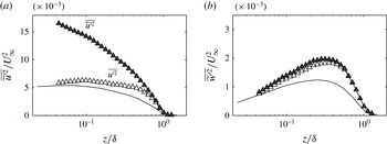
Streamwise (a) and wall-normal (b) turbulence intensity profile over the converging (symbols) region and smooth-wall reference (
 $-$
). ▵: Profile computed from Reynolds (convecting) fluctuation
 $u^{\prime }$
; and ▴: from spatio-temporal fluctuation
 $\widetilde{u}^{\prime }$
. Spatial-resolution correction is not applied in this figure.

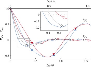
Spanwise slices through fluctuations self-correlation points at
 $z_{ref}/\unicode[STIX]{x1D6FF}=0.15$
over converging region (▴, blue and ▵, blue), diverging region (▾, red and ▿, red), and smooth wall (○). Open symbols: profiles computed using temporal fluctuations
 $R_{u^{\prime }u^{\prime }}$
. Closed symbols: profiles computed using spatio-temporal fluctuation
 $R_{\widetilde{u}^{\prime }\widetilde{u}^{\prime }}$
.

The difference between the two decomposition methods (4.1b
) and (4.1c
), also appears in the single-point velocity statistics. Figure 8(a,b) compares the streamwise and wall-normal turbulence intensities computed using both temporal fluctuation
 $u_{i}^{\prime }$
(open symbol) and spatio-temporal fluctuation
 $\widetilde{u}_{i}^{\prime }$
(closed symbols). These profiles are taken above the converging line at
 $y/\unicode[STIX]{x1D6EC}=0.5$
. The smooth-wall profiles are also included as the solid lines for comparisons. The abscissa of this figure are normalised by the local boundary layer thickness
 $\unicode[STIX]{x1D6FF}$
for scaling purposes, and the ordinate by the corresponding
 $U_{\infty }$
. Figure 8(a) clearly shows that the variance computed about the global mean
 $\overline{\widetilde{u}^{\prime 2}}$
is higher, with an intensity of more than three times of
 $\overline{u^{\prime 2}}$
at the measurement point closest to the surface. For the wall-normal velocity component however, since the time-averaged spatial variation
 $\widetilde{W}$
is very weak (and zero for
 $\widetilde{V}$
due to symmetry), the additional energy contribution from this time-invariant mode is insignificant. This is indicated by the minor difference in the wall-normal variances computed using the two different fluctuations. The effect of subtracting global/local mean also appears in spatial statistics such as the two-point velocity correlation. Figure 9 presents the correlation coefficient of streamwise velocity fluctuation, where all the profiles are computed about
 $z_{ref}/\unicode[STIX]{x1D6FF}(y)=0.15$
over the converging, diverging and the smooth-wall reference case. When the correlation is calculated using the fluctuations about the global mean
 $\widetilde{u}^{\prime }$
, a clear ringing effect with the wavelength corresponding to
 $\unicode[STIX]{x1D6EC}$
is observed in
 $R_{\widetilde{u}^{\prime }\widetilde{u}^{\prime }}$
. This is expected due to the occurrence of the positive/negative
 $\widetilde{u}^{\prime }$
over the riblets. When only considering the convecting turbulence
 $u^{\prime }$
however, the
 $R_{u^{\prime }u^{\prime }}$
profiles more closely resemble the accepted smooth-wall result. Nonetheless, no collapse is observed between any of the compared profiles. The average width of the streamwise turbulent events are noticeably narrower over the converging than the diverging region at this locally normalised wall height. From this observation we can see that the C–D riblets alter the instantaneous flow coherence beyond simply imposing a spanwise periodicity. We will further highlight this structural flow modification in § 5 from an instantaneous flow example. For the remainder of this paper, we will only consider the fluctuation about the local mean
 $u_{i}^{\prime }$
to analyse how the convecting turbulence has been altered by the C–D riblets.
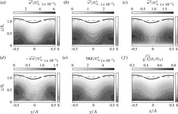
Contours of (a–c) streamwise, spanwise and wall-normal Reynolds stresses; (d,e) Reynolds shear-stress and turbulence kinetic energy; (f) root mean square of swirling strength over the C–D riblets. The smooth-wall profiles are included as narrow column axes for comparison.

4.3 Reynolds stresses and turbulence kinetic energy distribution
The distributions of Reynolds normal stresses for the current experiment are displayed in figure 10(a–c). The corresponding profiles for the smooth-wall base case are also displayed to the immediate right of each axis, labelled ‘S’. The pronounced spanwise variation is clearly apparent in all Reynolds stress components, where the converging (higher wall-drag) region experiences much stronger Reynolds fluctuations compared to the diverging region and the smooth-wall base case. The same behaviour was previously shown by Nugroho et al. (Reference Nugroho, Hutchins and Monty2013) over the same type of riblets for the streamwise fluctuating component. The increased magnitude in all turbulence intensities over the converging region clearly suggests that more energetic turbulent events occur in these regions. Figures 10(d) and 10(e) display the distribution of Reynolds shear stress (RSS)
 $-\overline{u^{\prime }w^{\prime }}$
and the turbulence kinetic energy (TKE) respectively, where TKE
 $=(\overline{u^{\prime 2}}+\overline{v^{\prime 2}}+\overline{w^{\prime 2}})/2$
. The spanwise periodicity in both statistics is certainly expected. Both RSS and TKE are much higher over the converging region (higher wall drag) throughout the boundary layer, compared to over the diverging (lower wall-drag) region. Regions of elevated RSS and TKE are also observed experimentally by Barros & Christensen (Reference Barros and Christensen2014) over complex heterogeneous roughness, where the most energetic locations coincide with the regions of lowered mean streamwise velocity, similar to what occurs over the C–D riblets. Finally, the root mean square of two-dimensional swirling strength
 $\unicode[STIX]{x1D706}_{ci}$
(described in Adrian, Christensen & Liu Reference Adrian, Christensen and Liu2000a
) is displayed in figure 10(f). This figure highlights the more frequent occurrence of intense small-scale turbulence over the converging region, which might indicate that the very-large-scale low-speed events that carry these small-scale vortical motions are preferentially arranged over the converging region.
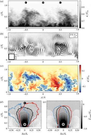
Representative example of instantaneous flow over the C–D riblets. (a) Total streamwise velocity
 $u$
. (b) The filtered in-plane total velocity
 $v_{f}$
and
 $w_{f}$
, marker
 $\otimes$
indicates the centre of the streamwise vortices. (c) Streamwise Reynolds fluctuation
 $u^{\prime }$
, black contour lines indicate
 $u^{\prime }=0.1U_{\infty }$
. (d) Conditional-average field over converging line and (e) smooth-wall.
 $+$
symbols indicate the reference point at
 $z_{ref}/\unicode[STIX]{x1D6FF}_{s}=0.15$
. Solid lines indicate contour of
 $\overline{u^{\prime }}_{cond}=-0.05U_{\unicode[STIX]{x1D70F}s}$
. No spanwise fluctuation
 $v^{\prime }$
condition (
 $-$
);
 $v^{\prime }<0$
(
 $-$
, blue);
 $v^{\prime }>0$
(
 $-$
, red).

5 Instantaneous flow structures
Figure 11(a) shows an example instantaneous streamwise velocity field
 $u$
over the C–D riblets. The figure highlights the most prominent feature in the
 $u$
fields, which is the tall eruption of low-speed fluid over the converging regions. Since this distinct event is observed in almost all instantaneous fields, it results in a strong periodicity in the mean streamwise velocity
 $U$
. There are rare instances where these eruption events exceed the wall-normal domain of the current measurement, but these events do not affect the single-point statistic results presented in the previous sections. Further visual inspection of the
 $u$
snapshots reveals that these
 $z$
-extended regions of low streamwise momentum tend to be tipped over transversely in the outer layer, which is also evidenced in figure 7.
The corresponding large-scale (filtered) in-plane velocities
 $v_{f}$
and
 $w_{f}$
are plotted in figure 11(b). These vectors are filtered using a Gaussian kernel with the size of
 $0.25\times 0.25\unicode[STIX]{x1D6FF}_{s}$
and standard deviation of 2. The vector grid has also been down-sampled for clarity of presentation. Several large-scale vortical motions can be distinguished in the figure, and the centre of several events are marked by the
 $\otimes$
symbols (markers are also drawn in figure 11
c). Note that these streamwise vortices are not the hairpin vortex signatures which are the typical small-scale features as mentioned by Adrian et al. (Reference Adrian, Meinhart and Tomkins2000b
), Tomkins & Adrian (Reference Tomkins and Adrian2003), Hutchins, Hambleton & Marusic (Reference Hutchins, Hambleton and Marusic2005). The large-scale filter kernel employed here would have attenuated these small swirling events, leaving only any residual large-scale tendency. Groups of the same sign swirling events however, can still manifest in these larger-scale rotations. These large-scale streamwise vortices can also be observed instantaneously in the smooth-wall flow fields as naturally occurring unstable motions, but with less magnitude and no preferred spanwise location. However, the directional pattern over the C–D riblets seems to have enhanced the frequency and magnitude of this motion so that it appears in many realisations with a preferred orientation. At
 $z/\unicode[STIX]{x1D6FF}=0.5$
for example, positive large swirling motions that occur in the region
 $0<y/\unicode[STIX]{x1D6EC}<0.5$
are statistically
 ${\sim}16\,\%$
stronger than those over the smooth wall. When comparing these instantaneous roll modes to the mean counter-rotating secondary flow shown in figure 6, one can deduce several major differences. Firstly, the diameters of the instantaneous motions are on average smaller than those found in the mean secondary flow that fills the entire boundary layer. Secondly, the centres of these motions do not always occur at
 $z/\unicode[STIX]{x1D6FF}_{s}\approx 0.3$
where the centres of the mean secondary flow appears, and they also tend to wander in the transverse direction. Furthermore, in many instances larger streamwise vortices appear to be one sided within adjacent converging regions. This non-symmetrical behaviour will be further described in § 6. Hence, contrary to the view afforded from the mean statistics (Nugroho et al.
Reference Nugroho, Hutchins and Monty2013), it can be concluded that these secondary flows happen intermittently with a multitude of length scales, frequencies and magnitudes, such that the
 $\unicode[STIX]{x1D6FF}$
-filling roll modes only exist in a time-average sense and are in fact a superposition of stronger individual streamwise vortices. Accordingly, the weakness of the mean roll modes could be somewhat misleading, since instantaneously the picture is one of much stronger individual events induced by the C–D texture.
The turbulence/temporal fluctuation
 $u^{\prime }$
of the same instance is displayed in figure 11(c). In the cross-stream view, the dominant features in these fields are the large plumes of low streamwise momentum ejecting from the wall, as observed previously by Hutchins et al. (Reference Hutchins, Hambleton and Marusic2005) in their sPIV measurement in inclined planes (
 $45^{\circ }$
and
 $135^{\circ }$
from
 $x$
-axis) over the smooth wall. As mentioned in § 4.2, removing the local
 $U$
from this spanwise periodic flow reduces the magnitude of the fluctuations (i.e. the values become less negative near the converging, and less positive near the diverging) especially closer to the riblets surface. Therefore, the negative
 $u^{\prime }$
structures can sometimes be seen to be detached from the wall as depicted by the structure at
 $y/\unicode[STIX]{x1D6EC}=-0.5$
. In non-homogeneous flows, subtracting the local mean from the total velocity essentially eliminates the stationary (time-average) spatial variation from the field. Therefore, for flows with less intense spatial heterogeneity such as over the realistic roughness analysed by Barros & Christensen (Reference Barros and Christensen2014), the instantaneous Reynolds fluctuation field
 $u^{\prime }$
will closely resemble the smooth-wall fluctuation field. Over the C–D riblets however, interesting features emerge from careful examination of the flow structures. The ejected low-momentum regions are typically ‘curled’ either clockwise or anticlockwise depending on their relative spanwise position over the riblets. This behaviour is highlighted by the contour lines of
 $u^{\prime }=-0.1U_{\infty }$
above the converging regions in figure 11(c). This large-scale curving behaviour can happen simultaneously in both directions similar to the feature above
 $y/\unicode[STIX]{x1D6EC}=-0.5$
, or more frequently as a one-sided tendency similar to the feature above
 $y/\unicode[STIX]{x1D6EC}\approx 0.5$
(another example can be seen in figure 7). The markers
 $\otimes$
also highlight the association between these inclined plumes to the large-scale instantaneous streamwise vortices.
To statistically assess the behaviour of these deformed low-momentum eruptions, we perform conditional averaging over the converging lines at
 $z_{ref}/\unicode[STIX]{x1D6FF}_{s}=0.15$
. The condition is based on the large-scale (filtered) streamwise velocity fluctuation
 $u_{f}^{\prime }$
, which is obtained by convolving the
 $u^{\prime }$
field with the same Gaussian kernel used in figure 11(b). The unfiltered
 $u^{\prime }$
fields are then averaged when
 $u_{f}^{\prime }(\text{converging},z_{ref})<-U_{\unicode[STIX]{x1D70F}s}$
. Here the filter size and the velocity threshold are arbitrarily chosen to represent a large-scale event with considerable energy, and the key results presented are not greatly altered by changes to these values. The result of this conditional averaging is shown in figure 11(d), where the grey background colour shows the averaged streamwise fluctuation
 $\overline{u^{\prime }}_{cond}$
and the black contour line indicates
 $\overline{u^{\prime }}_{cond}=-0.05U_{\unicode[STIX]{x1D70F}s}$
. The conditional-average field over the smooth wall is also compared in figure 11(e). Note that the smooth-wall average structure attains slightly better convergence since the samples can be taken across the entire homogeneous spanwise domain, whereas over the riblets we condition it above the converging lines at
 $y/\unicode[STIX]{x1D6EC}=\pm 0.5$
. Similar to cross-stream observations by Hutchins et al. (Reference Hutchins, Hambleton and Marusic2005), the average low-momentum region (darker colour) over the smooth wall is flanked by high-momentum regions (lighter colour). The superimposed in-plane conditional vectors also indicate the mean vortical motion that accompanies the low-speed upwash event. These naturally occurring behaviours are also observed in the conditional field over the converging region. Comparing the width of the contour however (see the black lines), reveals the narrower structure closer to the wall but noticeably wider further from the wall. Extra caution needs to be taken while interpreting the appearance of an average structure, since the observed shape can simply be the resultant statistical shape due to the superposition of several different events. To overcome this issue, we further divide the above conditional fields using the sign of the large-scale spanwise velocity fluctuation
 $v_{f}^{\prime }$
at the condition point. The same sorting is also done on the smooth-wall field for comparison. The red contour line in figure 11(d,e) indicates the
 $\overline{u^{\prime }}_{cond}=-0.05U_{\unicode[STIX]{x1D70F}s}$
contour that has positive spanwise velocity
 $+v^{\prime }$
, and the blue contour indicates the other half that has
 $-v^{\prime }$
. By sorting in this manner, the average structures over the C–D riblets clearly resemble the left/right leaning low-momentum features observed instantaneously in figure 11(b), highlighting their dominance within the flow field. Though this left/right leaning tendency is also weakly observed for the smooth-wall conditional averages in figure 11(e), it is much less pronounced than that above the riblets.
The corresponding filtered wall-normal velocity field
 $w_{f}$
of the example displayed in figure 11. The hatched regions show the area where
 $w_{f}$
is averaged to determine the instantaneous common flow direction within one C–D wavelength.

6 A closer look at the time-average secondary flow
It appears from figure 11 that the low-momentum regions above the converging part of the riblets undergo a lateral instability accompanied by predominantly one-sided arrangements of large-scale vortical motions. This suggests that the counter-rotating mode observed in the time-average view of figure 6 is not representative of the instantaneous vortex arrangement induced by the surface texture. Here we attempt to quantify this time-variant behaviour. Again, we will utilise conditional-averaging technique to establish the fractional time when the flow instantaneously exhibits a large counter-rotating motion within one C–D wavelength. Note that conditional averaging will essentially enforce a flow pattern that we are querying. Hence, careful interpretation is necessary, and our emphasis is on the proportion of snapshots that resemble the conditional features.
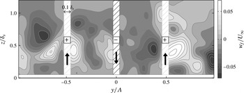
The velocity frames are sorted based on the instantaneous vertical velocity above the C–D-C regions. This process is illustrated in figure 12, where it shows the filtered wall-normal velocity
 $w_{f}$
corresponding to the example given in figure 11. This filtered component
 $w_{f}$
is averaged within a spanwise width of
 $0.1\unicode[STIX]{x1D6FF}_{s}$
(hatched region), to determine the instantaneous sign of the vertical flow in these three regions. In this particular example, the result is up-down-up since the resulting average is
 $+,-,+$
. All frames are then sorted based on this three-sign combination, giving
 $2^{3}$
possibilities. From this, conditionally averaged views of the cross-flow vectors
 $v$
and
 $w$
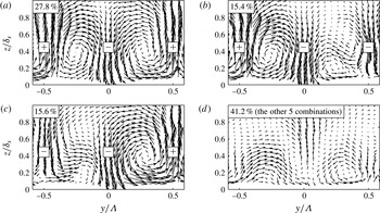
can be produced for each combination. Note that if all combinations are included, the conditional average will return the time-average secondary flow shown by the vectors in figure 6. Figure 13(a) displays the average in-plane velocities when the vertical signs over
 $y/\unicode[STIX]{x1D6EC}=-0.5,0,0.5$
are
 $+,-,+$
respectively. One can quickly notice that this pattern resembles the mean secondary flow, with the left side (
 $-0.5<y/\unicode[STIX]{x1D6EC}<0$
) exhibiting a
 $\unicode[STIX]{x1D6FF}$
-filling negative streamwise vortex and the right side (
 $0<y/\unicode[STIX]{x1D6EC}<0.5$
) showing the positive. Interestingly, this pattern is observed only for 27.8 % of the seven thousand acquired realisations. Figures 13(b) and 13(c), where the average
 $w_{f}$
are
 $+,-,-$
and
 $-,-,+$
respectively, also confirm that one-sided large-scale rotational motions occur more frequently (31 % of realisations) compared to the counter-rotating case shown in figure 13(a).
Conditional-average velocity vectors, sorted based on the sign (direction) of the vertical common flow above
 $y/\unicode[STIX]{x1D6EC}=-0.5,0,0.5$
. (a) Conditional vectors when average-
 $w_{f}$
are
 $+,-,+$
. (b,c) Conditional vectors when average-
 $w_{f}$
are
 $+,-,-$
and
 $-,-,+$
respectively. (d) Conditional vectors for the rest of the combinations. Figure is drawn to scale with figure 6.

Due to the forced condition, figure 13(a–c) displays at least one large-scale streamwise roll modes with the expected rotational sense. Figure 13(d) however, contains the other five combinations (i.e.
 $+,+,+$
;
 $-,-,-$
;
 $-,+,-$
;
 $-,+,+$
;
 $+,+,-$
). These lower percentage patterns are not individually plotted here for brevity. The average vortex pattern in these other combinations will either show the large-scale motions that turn the opposite to the time-average secondary flow, or consist of smaller rotational events. Again, these patterns are certainly enforced by the given condition events. However, it is definitely striking that these other five combinations (where each of the conditionally averaged field in no way resembles the time-averaged secondary flow) comprise 41.5 % of the total snapshots. The overall conclusion here would be that the large vortical events that give rise to the time-average secondary flow are to some extent intermittent in time (possibly also in the
 $x$
-direction), and that the time-averaging process has masked the often much stronger instantaneous large-scale roll modes that are induced by the surface texture.
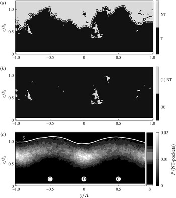
(a) Example of instantaneous field separated into turbulent/non-turbulent regions, with the interface outline superimposed. (b) The corresponding binary field of the non-turbulent pockets (assigned to be 1) and the rest of the field (assigned to be 0). (c) Probability of the non-turbulent pockets occurrence. The smooth-wall profile is included as a column axis.

7 The effect of C–D riblets in the intermittent flow region
Over the diverging part of the riblets (where the mean common flow down occurs), regions of fast moving fluid with a streamwise velocity approximately equal to the free-stream value are often observed deep within the boundary layer. These regions occur below the turbulent/non-turbulent (T/NT) ‘interface outline’ defined by Chauhan et al. (Reference Chauhan, Philip, de Silva, Hutchins and Marusic2014), and typically reside underneath the leaning low-momentum eruptions described in § 5. To illustrate this observation, figure 14(a) presents a realisation where the field has been separated into the turbulent (darker colour) and non-turbulent/free-stream (lighter colour) regions. These T/NT regions are identified using the kinetic-energy criteria of Chauhan et al. (Reference Chauhan, Philip, de Silva, Hutchins and Marusic2014), and the aforementioned interface outline is also highlighted. In this example, many ‘pockets’ of non-turbulent fluid (i.e. patches of small non-turbulent area which are fully encapsulated within the turbulent region) are present in the field of view. These pockets represent the potential flow regions that are perhaps drawn into the boundary layer by the large instantaneous motion discussed in § 5. The binary figure 14(b) highlights the occurrence of these NT pockets, where they are assigned the value 1 and the rest of the field are assigned 0. Viewing through multiple realisations, one can see a clear trend that patches of NT fluid often occur nominally above the diverging part of the riblets, although their locations vary slightly from frame to frame. This observation is then confirmed statistically by looking at the spatial probability
 $P$
of the NT-pocket occurrence, which is presented in figure 14(c). The probability is calculated by ensemble averaging the binary images of figure 14(b), and the result reveals a strong spanwise periodicity over the C–D riblets. The distribution of the smooth-wall base case is also included as the narrow axis immediately to the right, and labelled ‘S’. Over the converging region, the NT pockets seem to occur with similar frequency to the smooth-wall case. Over the diverging region however, this phenomena occurs twice as often. The observed large-scale engulfment of free-stream flow by the modified boundary layer might suggest that a certain degree of ‘forced mixing’ (Schubauer & Spangenberg Reference Schubauer and Spangenberg1960) has been imposed. This process will extract free-stream momentum towards the wall and facilitate the movement of the less energetic fluids. This possible mixing property opens a potential of using C–D riblets as a tool to delay boundary layer separation and to increase heat transfer without adding a significant amount of parasitic form drag.
8 Summary
A stereoscopic PIV experiment has been performed in a turbulent boundary layer over a converging–diverging riblet surface. The results and relevant discussions presented in this paper are summarised as follows,
-
(i) We categorise surface roughness based on their local
 $C_{f}$
isotropy and their drag homogeneity. The herringbone pattern discussed here is considered anisotropic (directional)-heterogeneous roughness. Although time-averaged secondary flows are present for both the isotropic and anisotropic spanwise heterogeneous categories, several noted differences (such as the surface characteristics and the secondary flow orientation) suggest that different mechanisms may be responsible for their generation.
-
(ii) The spanwise periodicity over the C–D riblets is pronounced, to the extent that the boundary layer thickness is locally altered. Accompanying this periodicity are mean counter-rotating roll modes. The orientation of these cellular roll modes can be inferred from assumption that upward/downward motions occur above region of flow convergence/divergence respectively. Strong spanwise variations are also observed in all Reynolds stress and the turbulence kinetic energy fields, where increased quantities are always observed above the converging regions. All second-order statistics are lower over the diverging region compared to the converging and the smooth-wall case.
-
(iii) Instantaneous analysis on the streamwise velocity fields reveal the consistent occurrence low momentum eruptions above the converging regions, as suggested by the time-average field. These large-scale events however, are often observed to be leaning in the transverse direction, and accompanied by large scale often asymmetric rotational motions. The conditional-average results reveal the dominance of these leaning structures in the flow field. This suggests that the large-scale low momentum regions that occur over the converging regions undergo a lateral instability that is stronger than that observed on the naturally occurring low momentum regions.
-
(iv) By employing a conditional sorting technique, we show that the instantaneous in-plane rotational motions resemble their time-average in-plane vectors for only 28 % of the fractional time. This observation perhaps offer an explanation regarding why this fully modified boundary layer is only accompanied by a very weak time-averaged ‘residual’ secondary flow. The present results suggest that the time-averaged
$V$
and
$W$
interpreted as mean secondary flows are perhaps an artefact of the averaging process arising from superpositions of much stronger turbulent events. -
(v) Large-scale free-stream engulfing behaviour is often observed associated with the common flow down tendency of the secondary flows. These motions cause a more frequent occurrence of free-stream pockets above the diverging region compared to the smooth-wall flow (without noticeable changes over the converging region). This observation might indicate an increase in flow mixing over the converging–diverging riblets.


Acknowledgements
The authors wish to thank the Australian Research Council for the financial support of this research. K.T.C., J. B. and G.P. gratefully acknowledge the support of the Air Force Office of Scientific Research under grant nos FA9550-10-1-0372 and FA9550-14-1-0101 (Dr D. Smith, Program Manager).