


The partisan primary system, which favors more ideologically pure candidates, has contributed to the election of more extreme officeholders and increased political polarization. It has become a menace to governing.
— Sen. Charles Schumer (D-NY)Footnote 1
The divergence between candidates and legislators from the two major parties is an enduring feature of the American political landscape (Ansolabehere, Snyder, and Stewart Reference Ansolabehere, Snyder and Stewart2001; Bonica Reference Bonica2013; Poole and Rosenthal Reference Poole and Rosenthal1984, Reference Poole and Rosenthal1997), and the fact that polarization is at historically high levels is a significant concern for scholars and observers of democratic governance, representation, and public policy (Hacker and Pierson Reference Hacker and Pierson2006; Mann and Ornstein Reference Mann and Ornstein2013; McCarty, Poole, and Rosenthal Reference McCarty, Poole and Rosenthal2006, Reference McCarty, Poole and Rosenthal2013). Indeed, politicians and the popular press often lay much of the blame for this phenomenon on partisan primary elections, typically employing a simple, intuitively appealing argument: Candidates take extreme positions because they must appeal to partisan primary voters, whose preferences are more extreme than those of voters in the general election.
Political scientists have tested this argument, finding that while there is some evidence to suggest that primary elections promote extremism, the empirical record is mixed. Extremists are more likely to win congressional primaries than moderates (Brady, Han, and Pope Reference Brady, Han and Pope2007), and legislators elected under closed primaries take more extreme positions than legislators elected under open primaries (Gerber and Morton Reference Gerber and Morton1998). But other analyses find that polarization is largely unrelated to the introduction of direct primaries (Hirano et al. Reference Hirano, Snyder, Ansolabehere and Hansen2010) and to the variation in the openness of primaries across states (McGhee et al. Reference McGhee, Masket, Shor, Rogers and McCarty2014). At best, primaries may cause polarization under limited circumstances (Bullock and Clinton Reference Bullock and Clinton2011), and despite the divergence of candidate positions, general elections nevertheless exert nontrivial pressure on candidates to moderate (Hall Reference Hall2015; Hirano et al. Reference Hirano, Snyder, Ansolabehere and Hansen2010). These findings seem puzzling in light of the basic theory of representation at the heart of this literature that the extremity of primary electorates should directly affect the extremity of party candidates.
How, then, should we understand the causal relationship between primary elections and candidate positioning? I examine the connection, both theoretically and experimentally, by comparing elections with and without primaries while holding other features of the electoral environment constant, including preferences and information. The analysis focuses on a particular aspect of primary elections—how the introduction of voters in the candidate selection process affects strategic competition between parties—while abstracting away from many other considerations that might also affect polarization.Footnote 2
The contribution of this paper is to develop a more nuanced theoretical understanding of the relationship between primaries and polarization than is portrayed in the existing literature. The key theoretical innovation is to move beyond preference-based explanations by treating beliefs as a primitive of the model in a way that is ruled out by standard equilibrium analysis in complete information environments. I show that primaries can cause polarization or moderation, depending on candidates’ beliefs about opposing voters’ strategic behavior—even when preferences are held constant. To generate this insight, I rely on ideas from behavioral game theory, which retains much of the theoretical apparatus from standard game theory while allowing for key departures (Camerer Reference Camerer2003). Specifically, I allow players to have “incorrect” or “nonequilibrium” beliefs about others’ actions (Crawford, Costa-Gomes, and Iriberri Reference Crawford, Costa-Gomes and Iriberri2013), but assume they are nevertheless strategic in the sense that they best respond to what they think other players do (Camerer, Ho, and Chong Reference Camerer, Ho and Chong2004; Nagel Reference Nagel1995; Stahl and Wilson Reference Stahl and Wilson1995). The analysis demonstrates that changes in preferences alone are not the only cause of polarization. Instead, beliefs and expectations about the strategic behavior of others play important roles in conditioning the effect of institutions.
I then turn to the laboratory and conduct a series of experiments to test the effects of primaries on candidate positions and to distinguish between behavioral assumptions. The chief advantage of the laboratory for theory testing is control (Aldrich and Lupia Reference Aldrich, Lupia, Druckman, Green, Kuklinski and Lupia2011; Falk and Heckman Reference Falk and Heckman2009; Morton and Williams Reference Morton and Williams2010), so we can be confident that the observed behavior occurs under the conditions specified by the theoretical model. Importantly, subjects face the same key tradeoff in the experiment as the actors do in the theoretical model between increasing the favorability of winning outcomes versus increasing the probability of winning. In the lab, theoretically relevant quantities of interest that are difficult to measure using observational data with any accuracy or without strong assumptions (in particular, preferences and positions) are also known exactly. Furthermore, experimental manipulations permit tests of mechanisms not possible using observational data. Thus, laboratory experiments are ideal for theory testing given their high internal validity.Footnote 3
The key finding from the experiment is that primaries appear to cause a kind of ideological purity rather than greater extremism. Regardless of whether there is a primary election or not, I find that subjects take positions that diverge significantly from the median voter’s position. This finding lends support for the behavioral theory. However, the extent to which primaries cause polarization is limited. Greater polarization only occurs without feedback such that candidates cannot learn about the behavior of others, and this polarization happens because voters tend to select extremists over moderates, even though candidate positions do not vary with the election format. More precisely, the analysis reveals that voters do not support party extremists or party moderates unconditionally. Instead, they select candidates with intermediate positions, consistent with their own subjective beliefs about optimal candidate positions, approximately halfway between the median voter and their own party’s ideal point. This behavior generates a greater concentration of candidate positions around an average that diverges from the median voter. Hence, greater ideological homogeneity reinforces, rather than exacerbates, polarization.
RELATED LITERATURE
My analysis follows a long tradition of using spatial voting models to understand elections. Although existing spatial models predict candidate divergence in elections with primaries, they do so in isolation and do not compare them explicitly to elections without primaries (Aronson and Ordeshook Reference Aronson, Ordeshook, Niemi and Weisberg1972; Coleman Reference Coleman, Niemi and Weisberg1972; Owen and Grofman Reference Owen and Grofman2006).Footnote 4 These models also assume that general election outcomes are probabilistic, which is theoretically consequential because the mechanism they rely on to produce divergence is the combination of policy motivations and uncertainty about which candidate will win the general election—the same forces that generate incentives for candidate divergence in the absence of primaries (Calvert Reference Calvert1985; Wittman Reference Wittman1983). Thus, it is unclear from the literature whether polarization can be traced to any distinctive features of primaries per se, as electoral institutions. By explicitly comparing institutions, my analysis speaks directly to the connection between primaries and polarization.
Existing theoretical models of two-stage elections also typically maintain the assumption that all political actors, candidates as well as voters, are strategic and forward-looking (e.g., Owen and Grofman Reference Owen and Grofman2006). Several models consider the issue of raiding and crossover voting in open primaries (Cho and Kang Reference Cho and Kang2014; Chen and Yang Reference Chen and Yang2002; Oak Reference Oak2006), which requires a fairly high degree of strategic sophistication, but this kind of behavior is outside the scope of my analysis. My results also differ from Adams and Merrill (Reference Adams and Merrill2014), who find that strategic versus expressive voting both generate divergence, but in their model candidates are office-motivated and vary in their campaign skills. In contrast to the preponderance of existing formal models, I take a behavioral (i.e., bounded rationality) approach advocated by Simon (Reference Simon1955), Ostrom (Reference Ostrom1998), Bendor (Reference Bendor2010), and others. I do so by explicitly allowing for sincere (myopic) voting as well as subjective beliefs that are inconsistent with observed behavior.
This paper is also related to two distinct literatures in experimental political science. The experimental literature on candidate positioning in two-party elections finds a strong tendency for candidates and election outcomes to converge to the median voter’s position and, more generally, to the Condorcet winner under a variety of conditions, including incomplete information (Collier et al. Reference Collier, McKelvey, Ordeshook and Williams1987; McKelvey and Ordeshook Reference McKelvey and Ordeshook1982, Reference McKelvey and Ordeshook1985). An exception is Morton (Reference Morton1993), in which candidates are ideological and voting is probabilistic. The other related literature, on strategic voting, generally finds little (at best, mixed) evidence for voter sophistication in the early stages of a multistage voting agenda or election contest (Cherry and Kroll Reference Cherry and Kroll2003; Eckel and Holt Reference Eckel and Holt1989; Herzberg and Wilson Reference Herzberg and Wilson1988; McCuen and Morton Reference McCuen and Morton2010; Plott and Levine Reference Plott and Levine1978; Van der Straeten et al. Reference Van der Straeten, Laslier, Sauger and Blais2010).Footnote 5 Taken together, these previous studies raise doubts that voters will be highly strategic (even if candidates are), calling into question theories predicated on voter rationality and strategic sophistication.
THEORETICAL FRAMEWORK AND ANALYSIS
I consider an environment with two parties, Party L and Party R, competing to win a single office. Candidates choose positions in a one-dimensional policy space, and the winning candidate’s position is implemented as the policy outcome. In the electorate, there are an equal number of voters in each party and a set of independent, nonpartisan “swing” voters. Candidates and voters alike are entirely policy-motivated, caring only about the location of the policy outcome w  $\ \in \mathbb {R}$. The incentive to win office is therefore purely instrumental in this model, which departs from the usual Downsian office motivations. Parties are completely homogeneous, as candidates and voters belonging to the same party both care about policy and have the same ideal point. Thus, there are three ideal points in the model: θL for members of Party L, θR for members of Party R, and θM for the electorate’s median voter, where θL < θM < θR. I assume that preferences are symmetric and single-peaked. Specifically, in the experimental implementation, all actors have linear loss utility functions, u i(w) = K − |w − θi|, for i ∈ {L, M, R} and some constant K > 0. Preferences are also common knowledge, so the election takes place under conditions of complete information.
There are two types of elections. In one-stage elections (1S), each party has one candidate and their positions are c L and c R, respectively, and there is one round of majority rule voting to select the winning candidate. In two-stage elections (2S), each party has two candidates (denoted c L1 and c L2 for Party L, c R1 and c R2 for Party R) who first compete in intraparty elections (the primaries). The candidates who win their respective party primaries then compete in a second-round election (the general election) to select the winning policy w. In other words, the parties hold simultaneous “closed” primaries in which the voter with ideal point θL chooses c L ∈ {c L1, c L2} for Party L while the voter with ideal point θR chooses c R ∈ {c R1, c R2} for Party R. In the general election, the median voter with ideal point θM chooses the election outcome from the two candidates selected by the parties’ respective median voters, w ∈ {c L, c R}.
To generate predictions about candidate positioning and to identify the effects of the election format, I consider a variety of alternative behavioral assumptions. I begin with standard game theoretic analysis, applying Nash equilibrium as the solution concept. Since I am interested in making behavioral predictions, the interpretation of Nash equilibrium is worth a brief discussion. One way to interpret Nash equilibrium is to think of it as an idealized set of assumptions such that actors are not only fully rational but also that their rationality is common knowledge (Aumann and Brandenburger Reference Aumann and Brandenburger1995). In this interpretation, we can think of political actors as forming beliefs about others’ current and future behavior (as well as beliefs about beliefs and rationality, and so on) that are fully consistent with players’ actual strategies and behavior. Alternatively, Nash equilibrium can be interpreted as merely representing a stable outcome in which strategies are mutual best responses, without necessarily invoking an epistemic or belief-based justification of how individuals make decisions in games. The latter approach, however, does not make clear cut predictions about how games are played before an equilibrium state is reached. Nevertheless, under a wide variety of learning models, experience can lead play to converge to Nash equilibrium (Fudenberg and Levine Reference Fudenberg and Levine1998), and the role of experience can be investigated experimentally.
Relaxing the Nash assumption of the mutual consistency of beliefs and actions generates an interesting variety of behavioral possibilities. In my analysis, I first explore the implications of voter sophistication for candidate positioning while holding candidate rationality constant. If voting is “sincere,” then primary elections produce more polarized candidates than voting that follows an equilibrium strategy. I then consider another departure from standard assumptions: beliefs that some players make mistakes in choosing their positions. They might do so for any number of reasons, such as miscalculating the optimal position, misjudging or underestimating the rationality of others, or having preferences over outcomes of the game that are not fully captured by their material payoffs. Strategically sophisticated players, recognizing that there are other players who make mistakes, will then choose positions that differ from the Nash predictions—in the direction of their parties’ ideal points—but that are optimal given their own beliefs about the distribution of opponents’ positions. Introducing noise or the possibility of mistakes generates divergence in both one-stage and two-stage elections, despite complete information about preferences.
With noise, the effect of introducing a primary election is more nuanced. Similar to the case in which candidates do not make mistakes, the optimal positions depend critically on the behavior of primary voters. If voters choose moderate primary candidates, then two-stage elections will generate greater convergence of candidate positions than in one-stage elections. However, if voters choose extreme primary candidates, then candidates in two-stage elections will be more polarized than candidates in one-stage elections. There is also a third possibility: If voters form their own beliefs about the position most likely to maximize their expected utility and vote for candidates closest to this position, then the degree of candidate divergence in two-stage elections is increasing in what we might call voters’ belief-induced ideal points. Behavioral game theory thus establishes a critical link between candidates’ beliefs about opponents’ primary voting behavior and the effect of primaries.
Candidate Equilibrium with Fully Strategic Voters
Standard equilibrium analysis leads to identical predictions for both one-stage and two-stage elections. This is because, in any equilibrium, the winning candidate’s position is the median voter’s ideal point. In one-stage elections, the logic is straightforward. The median voter chooses the party candidate closest to his or her ideal point as the winning candidate, so if one candidate adopts θM as a campaign position, no other position can defeat it. In the unique equilibrium of the one-stage election game, both parties’ candidates must choose c L = c R = θM. If not, either the winning party’s candidate could do better by finding a position closer to her ideal point while still winning the election or the losing candidate can find a position that wins the election, thereby obtaining a better policy outcome for herself. Thus, w = θM is the unique equilibrium policy outcome.
In two-stage elections, the outcome is the same, but the equilibrium strategies of the primary voters must be specified. Given a set of candidate positions and voters’ expectations that the general election median voter will choose the more moderate of the parties’ candidates, a primary voter’s strategy is to choose the candidate closest to her ideal point as long as she believes the candidate will also win the general election (and in equilibrium, the voter’s beliefs about which candidate will win are correct). Because candidates and voters have the same preferences, the incentives guiding optimal candidate strategies in the one-stage election are similar to those that guide rational voting behavior in two-stage elections: if offered the same choices, candidates and voters would choose the same position (the only difference is that candidates can choose any position while primary voters’ choices are constrained).
In any equilibrium of the two-stage election game, there must be at least one candidate from each party located at θM, so primary voters will always be observed choosing the moderate candidate along the path of play. If so, both parties’ primary voters will select a candidate at the median voter’s ideal point and the policy outcome is therefore w = θM. Ruling out other possible outcomes then follows from the same logic as in the nonprimary election. Assuming fully strategic behavior from voters therefore predicts full convergence to the median voter’s position in both one-stage and two-stage elections.
Prediction 1. If voters and candidates are rational, forward-looking agents and form correct beliefs about others’ behavior, then (a) the moderate candidates from each party will adopt the median voter’s position and (b) primaries will have no effect on the polarization of candidates in the general election.
Candidate Equilibrium with Sincere Voters
I next consider the possibility that primary voters are myopic and vote “sincerely.”Footnote 6 I assume that sincere voters simply vote for the candidate closest to their ideal points, so they are myopic in the sense that they fail to recognize that the candidate’s chances of winning the general election affect the policy outcome (and hence their payoffs). With myopic voters, the two-stage election game has multiple equilibria in which candidates take divergent positions while the equilibrium of the one-stage election game remains the same (full convergence, since there are no primary voters).
In any equilibrium of the two-stage election game with sincere voters, candidates within each party must adopt the same position, and opposing party candidates must be equidistant from the median voter. Specifically, an equilibrium is characterized by the condition that c L1 = c L2 = θM − δ and c R1 = c R2 = θM + δ, where δ ≥ 0 denotes some amount of divergence between candidates. The median voter’s strategy is to select the candidate closest to her own ideal point, breaking ties in favor of each party with equal probability.Footnote 7 The result of the general election is therefore a lottery over w ∈ {θM − δ, θM + δ}, and the expected value of the outcome is the median voter’s position, E[w] = θM. Any candidate who adopts a more extreme position would, at best, be able to win their own primary but then would lose the general election with certainty. Moving to a more moderate position would not change the result of the primary and thus would not change the general election result either. Since no candidate can obtain a better policy outcome by unilaterally adopting a different position, campaign promises characterized by intraparty convergence and interparty symmetric divergence constitute an equilibrium of the primary election game with sincere voters. The basic intuition underlying this result is that due to the myopic behavior of sincere primary voters, intraparty competition limits any one candidate’s ability to moderate their party’s position in the general election. Thus, in contrast to full convergence in one-stage elections, any amount of divergence can be supported in two-stage elections.
Prediction 2. If candidates are rational and forward-looking but primary voters “sincerely” select candidates closest to their own ideal points, then (a) candidates from each party will take positions that diverge from the median voter by the same amount in two-stage elections, and (b) winning candidates will be weakly more polarized in two-stage elections than in one-stage elections, while candidates in the latter will converge to the median voter.
Candidate Best Responses to Out-of-Equilibrium Beliefs
The previous sections assumed that candidates correctly anticipate whether voters use either Nash or sincere voting strategies and that their beliefs about other candidates are consistent with those candidates’ actual behavior. That is, if candidate j chooses the platform c j, then candidate i must believe with certainty that c j must really be j’s position. However, this mutual consistency of candidates’ beliefs and actions might break down in a number of ways. Candidates are likely to face cognitive constraints, they may engage in incomplete strategic reasoning, or they may doubt the rationality of other candidates. In this section, I apply the notion of limited strategic sophistication motivated by level-k models in behavioral game theory (Crawford Reference Crawford2003; Nagel Reference Nagel1995; Stahl and Wilson Reference Stahl and Wilson1995), positing that candidates have some (possibly arbitrary) beliefs and analyze the best response to such beliefs.Footnote 8
To model this, let candidate i’s beliefs about the positions of candidates from the opposing party j ≠ i be given by the cumulative distribution F(c j). Importantly, these beliefs need not be accurate. For instance, if j’s true position is c j = 0, candidate i might believe that c j is uniformly distributed between −1 and 1. We can think of the distribution F(c j) as representing subjective beliefs that will typically not satisfy the equilibrium consistency requirement.Footnote 9
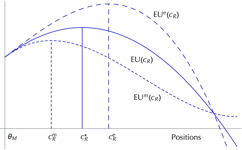
By relaxing the standard equilibrium assumption of belief consistency, an otherwise expected utility maximizing candidate will choose a position that diverges from the median voter’s ideal point. The reasoning is as follows. If a candidate believes there is some possibility that the opposing candidate’s position diverges from the median voter, then it cannot be optimal for a policy-motivated candidate to choose a platform exactly at the median voter’s ideal point. Instead, the candidate will choose a position that trades off some probability of winning against potential policy gains obtained from choosing a position closer to his or her own ideal point. To illustrate this concretely, suppose that θR = 1, the left party’s ideal point is θL = −1, the median is θM = 0, and F(c L) is a uniform random variable, c L ~ U[ − 1, 0]. With linear loss utility, the optimal position that balances this tradeoff is  $c_R^\ast = \frac{1}{3}$. This is illustrated by the solid line showing the expected utility function EU(c R) in Figure 1.Footnote 10 While this logic is similar to the tradeoff found in Calvert (Reference Calvert1985) and Wittman (Reference Wittman1983), the important distinction is that the source of uncertainty in this model is entirely about opponents’ behavior rather than about voters or preferences. Moreover, candidate positions are responsive to beliefs such that when a candidate is more likely to expect her opponent to be extreme (i.e., when F(c j) puts more weight on extreme positions), then she herself will take a position with greater divergence from the median voter in response.
Comparison of Candidate Expected Utility in One-Stage and Two-Stage Elections as a Function of Out-of-Equilibrium Beliefs and Opponents’ Primary Voting Behavior

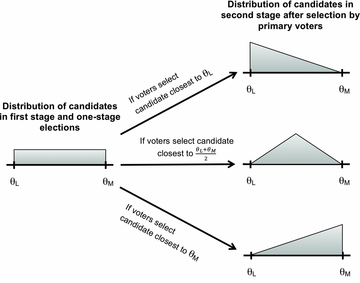
Next, I consider how these beliefs about opposing candidates’ positions interact with the type of election. The main result is that the effect of primaries will depend on the candidates’ beliefs about the opposing party’s primary voters. The baseline for comparison is a one-stage election with opponents drawn from the belief distribution F(c j). For the purposes of exposition, suppose that F(c j) is uniform as in the example just given and as shown in the left side of Figure 2, so the candidate’s best position is the one that maximizes the same expected utility function EU(c R) mentioned previously in Figure 1.
Comparison of Beliefs in One-Stage and Two-Stage Elections as a Function of Opponents’ Primary Voting Behavior

In a two-stage election, it is not the original distribution of candidates F(c j) that matters, but beliefs about which candidate will emerge from the primary election. Let G(c j) denote this latter set of beliefs about the candidate selected by the opposing party’s primary—the candidate that i expects to face in the general election. We can think of the primary election as a selection mechanism or filtering process that affects whether a party’s candidate is systematically more or less extreme than the party’s initial set of candidates.
More precisely, suppose that both of the opposing party’s candidates are independently drawn from F(c j). Now consider how primary voting behavior affects G(c j) and, in turn, candidates’ positions. If j’s primary voters unconditionally select the more extreme candidate (as they would if they voted sincerely), then party j’s candidate in the general election will be the more extreme of two independent draws from F(c j). This results in a distribution G(c j) that is skewed more toward j’s own ideal point than F(c j), as shown by the triangular distribution in the upper-right of Figure 2 when F(c j) is uniform.Footnote 11 When voters choose extremists, primaries generate incentives for greater extremism than in one-stage elections, as illustrated by the upper-dashed expected utility function EU e(c R) in Figure 1.
The flip-side of this is that if j’s primary voters select the more moderate candidate (as they would in equilibrium), they generate incentives for greater moderation than in one-stage elections. This is because party j’s general election candidate will be the more moderate of two independent draws from F(c j), resulting in a distribution of beliefs G(c j) that is skewed more toward the median voter than F(c j). This is shown in Figure 2 by the triangular distribution in the bottom right.Footnote 12 When the probability of facing an extremist opponent is lower, a candidate must moderate their position in response, which is shown by the lower-dashed expected utility function EU m(c R) in Figure 1.
These are not the only possibilities, as primary voters might also behave in other ways. For example, a fairly sophisticated voter might reason in the same way as a candidate and form the same beliefs G(c i) based on expectations about opposing primary voters. To generalize this idea, suppose that a voter has a belief-induced ideal point c*j and always votes for the candidate in the primary whose position is closest to c*j (sometimes this will be the moderate and sometimes the extremist). The result is a distribution of primary candidates G(c j) that has greater mass closer to c*j than F(c j) does. If c*j happens to be the midpoint between the voter’s ideal point and the median voter, G(c j) will be the symmetric triangular distribution in the middle-right of Figure 2. Note that while the mean of this distribution is the same as the original distribution F(c j), it has lower variance.Footnote 13 Primary elections may therefore also have the effect of reinforcing ideological purity (i.e., increasing homogeneity) within parties even when there is no discernible effect on average candidate positions (i.e., absent changes in polarization).
In contrast to standard equilibrium analysis, which predicts full convergence, a simple model with out-of-equilibrium beliefs generates divergence in candidate positions, even in the absence of primaries and with complete information about preferences. Moreover, the effect of primaries varies with candidates’ expectations about the opposing party’s voting behavior. Primaries can indeed cause greater polarization (but only if primary voters select sufficiently extreme candidates), cause greater moderation (if primary voters select moderates), or cause increased intraparty homogeneity (if voters select on the basis of intermediate belief-induced ideal points). Thus, the behavioral theory identifies how the effect of primaries depends on the connection between beliefs and behavior rather than on preferences alone.
Prediction 3. If candidates have out-of-equilibrium beliefs about the distribution of opposing candidates, then (a) candidate positions will diverge from the median voter’s ideal point in both one-stage and two-stage elections, (b) the direction of the effect of primary elections on candidate polarization depends on expectations about voting behavior, and (c) polarization in two-stage elections is increasing in the expected extremity of candidates selected by the opposing party’s primary voters.
EXPERIMENTAL ANALYSIS
The theoretical analysis generated a set of competing predictions about the effect of primaries as a function of alternative behavioral assumptions. If all players are fully strategic, then we should observe full convergence to the median voter’s position and primaries should have no effect (Prediction 1). If candidates are strategic but voters are not, then we should observe candidate divergence only in two-stage elections but not in one-stage elections (Prediction 2). If the behavioral theory has merit and candidates have subjective beliefs about their opponents’ positions, then polarization, moderation, or increased homogeneity are possible depending on voter behavior (Prediction 3). Which set of assumptions is a better reflection of how humans behave is ultimately an empirical question, and thus, I turn to the lab to distinguish between the competing theories.Footnote 14
Procedures
The experiment was conducted at the Pittsburgh Experimental Economics Laboratory and involved a total of 182 participants drawn primarily from the university’s undergraduate population. Each session involved 14 participants, and each subject participated in one session of either the 1S election treatment (six sessions) or the 2S election treatment (seven sessions). At the beginning of each session, following standard laboratory procedures, subjects gave informed consent, the instructions were read out loud to induce public knowledge, and subjects answered a set of questions about the rules on their computers to ensure comprehension.Footnote 15 The interface was computerized and programmed using the software z-Tree (Fischbacher Reference Fischbacher2007). Each session took about an hour and a half to complete, and subjects earned an average of $21.05 (including a $7 show-up fee).
Subjects participated in a total of 40 elections, and the instructions emphasized that each election was to be treated as a “separate decision task.” For each election, subjects were divided into two groups of seven participants, and every member of a group had the same payoff function and ideal point.Footnote 16 Throughout the experiment, the policy space was the set of integers from 1 to 200, and payoffs were given by the linear loss function 200 − |w − θi|.Footnote 17 The parties’ ideal points were located symmetrically from the median voter’s ideal point θM such that θL = θM − d, θR = θM + d, and d ∈ {50, 75}. The numerical value of θM varied from election to election, while the exact sequence of values was identical across sessions and treatments.Footnote 18 Payoffs were denominated in “points” and converted to cash by dividing by 10 and rounding to the nearest quarter. Given this conversion rate, the range of possible monetary payoffs for each election was between $0 and $20. The final payment was determined by randomly selecting one election to count from the entire session and then adding the show-up fee.
At the beginning of each election period, subjects first learned the position of every player’s ideal point. Every subject then chose a policy position (referred to as their “campaign promise”), and they were informed that if their campaign promise was selected as the winning position, it would affect every other subject’s payoff. After subjects chose their campaign promise, the computer then randomly selected candidates from each group: one candidate from each group in the 1S election and two candidates from each group in the 2S election, with each group member equally like to be selected and the selection of candidates independent across election periods. The rest of the subjects were assigned to the role of a voter in that election. Thus, at the beginning of each election, every subject was a potential candidate and did not know whether he or she was a candidate until after submitting a campaign promise.Footnote 19
Once the candidates were selected, the game proceeded to the voting stages. In the 2S election, voters first chose between one of their group’s two candidates by majority rule. Each primary (first stage) vote is held simultaneously, and neither party knew the positions of the other group’s candidates while voting. Abstentions were not allowed. After each group selected its nominee, a second round of voting took place to choose the winning policy from the two groups’ nominees. All voters participated in this second round, which was effectively the “general election.”Footnote 20 In contrast to the 2S election treatment, the 1S election treatment featured only one round of voting in which every voter participated.
The median voter in the general election in both the 1S and 2S election treatments was a computer voter who had a distinct ideal point and, as the instructions explained to subjects, similar to Morton (Reference Morton1993), was “like a robot programmed to always vote for the candidate whose campaign promise gives it the higher payoff value.” In the case of ties, the computer voted for each candidate with equal probability. The subjects were informed of the computer voter’s ideal point before every election.
The 40 elections within each session were divided into two parts, where each part varied the type of feedback subjects received. Part 1 consisted of ten elections without any feedback.Footnote 21 Part 2 consisted of 30 elections with feedback provided to subjects after each election. The information subjects received included the positions of the subjects who were selected as candidates, the number of votes for each candidate, the winning position, and the payoff from the final outcome. Within each part, I varied the distance between the groups’ ideal points by dividing each set of elections into two halves. In the first half, the left and right groups’ ideal points were 100 units apart (d = 50), while in the second half, they were 150 units apart (d = 75). Note that both of these within-subjects manipulations varied ancillary assumptions (feedback and distance between ideal points) and therefore serve as robustness checks. The experimental manipulation of theoretical interest is the between-subjects manipulation of the electoral institution.
Electoral Dynamics
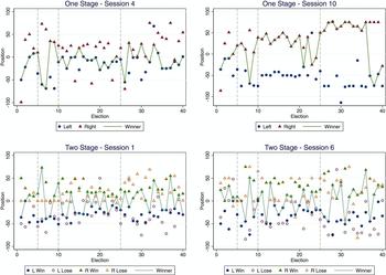
To get a sense of the kinds of promises candidates make and whether moderates or extremists win elections, Figure 3 presents the sequence of candidate positions and outcomes for selected sessions (two 1S sessions and two 2S sessions). The horizontal axis indicates the election, and the vertical axis indicates the promises of the subjects selected as the candidates. These positions are adjusted (centered) so that the general election median voter’s position is zero. The vertical lines indicate when the electoral conditions change in terms of feedback and the distance between the parties’ ideal points. General election candidates are depicted using solid shapes (candidates in 1S elections and the primary winners in 2S elections) while primary candidates who lost the first stage election are depicted with hollow shapes. The winning position of the general election is shown by the solid line. Although the dynamics of each session differ, these plots reveal several noteworthy patterns.
Sample Session Dynamics

First, the positions of candidates from the two parties clearly diverge from the median voter’s position. This is true for both 1S and 2S elections, and it appears to persist over the course of the experiment even after subjects gain considerable experience. In session ten (1S), for example, the candidates from each party choose positions close to their own ideal points, and polarization between the candidates’ positions increases when the underlying preference polarization increases. Along with divergence, there also appears to be substantial heterogeneity and fluctuation in candidate positions.Footnote 22
Second, while the general election candidate closer to the median voter’s position generally wins, it is rare for the winning candidate to be located exactly at the predicted equilibrium position. Even in session 4 (1S), in which the electoral outcome appears most frequently near the median voter’s position, the winning candidate is located at the median’s position in only three elections (in another eight elections, the winning candidate is ±1 from the median voter’s position). In session ten, the winning candidate usually appears to be just barely closer to the median voter than the losing candidate.
Third, primary voters are inconsistent in selecting either extreme or moderate candidates. Notably, there are several candidates in two-stage elections who locate at exactly the median voter’s position yet lose the primary. In session one, there were 12 out of 14 such candidates, and in session six, there were six out of ten. While this could suggest that primary voters prefer extremists, there are also many elections in which the more moderate candidate wins. For example, in election 11 of session six, the left party candidate at −30 defeated the candidate at −45, and the right party candidate at 20 defeated the candidate located at 50, with the right party candidate (who is closer to the median voter) winning the general election. Indeed, Figure 3 depicts losing candidates in primary elections on either side of the parties’ winning candidates (indicated by the fact that the hollow candidate markers appear both above and below the solid ones).
These sample dynamics suggest that standard game theoretic analysis poorly predicts candidate positions and voting behavior in the experiment. Whereas equilibrium predicts complete candidate convergence in both 1S and 2S elections, I find that candidates’ positions instead diverge. The considerable heterogeneity in candidate positions and the selection of extreme candidates by primary voters indicate that behavioral game theory and nonequilibrium analysis may be useful tools for understanding the consequences of electoral institutions. Of course, Figure 3 only provides a snapshot of experimental behavior. The remainder of the analysis demonstrates that many of the patterns described above generalize across subjects and sessions.
Candidate Positions
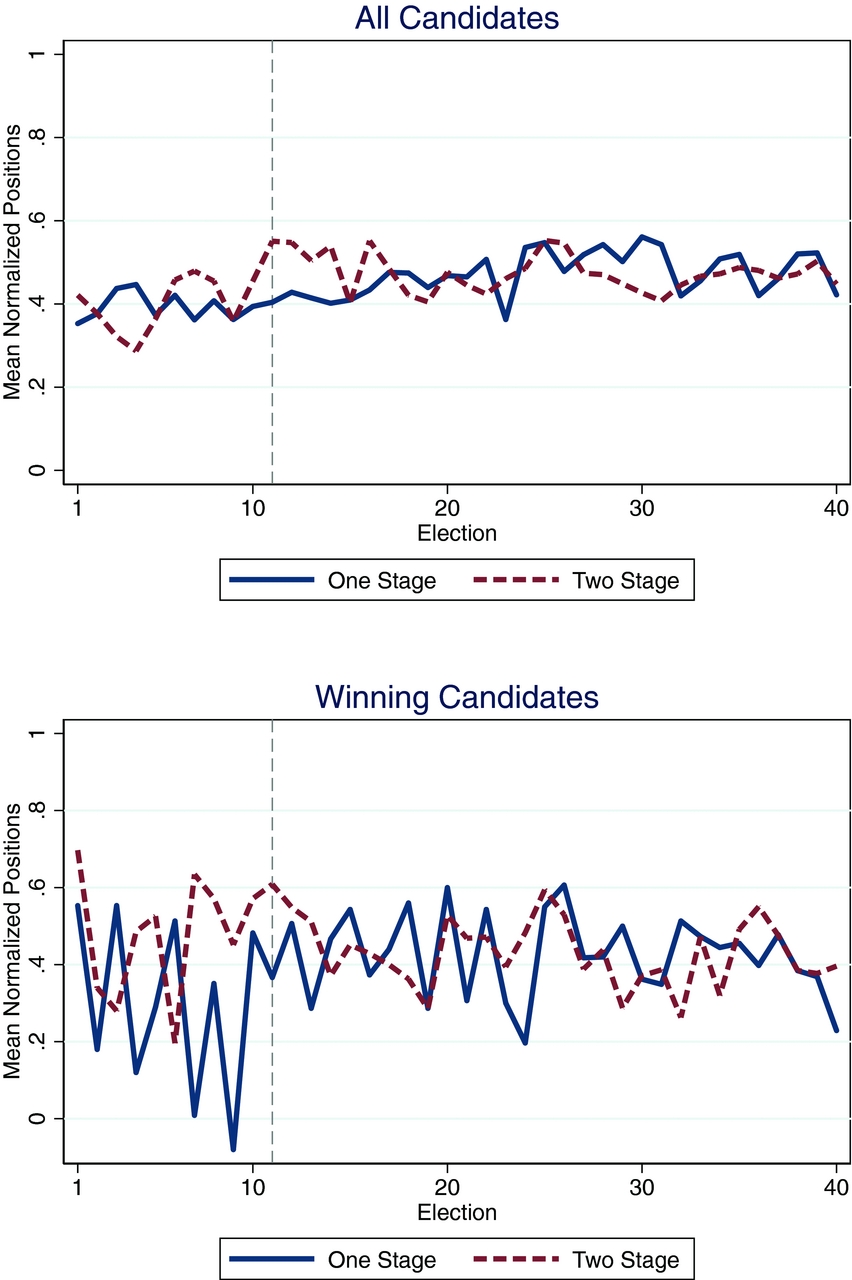
Figure 4 shows the average positions over time and by election format for all candidates (top panel) and for winning candidates (bottom panel). In the remainder of the analysis, I measure the extremity of a candidate’s position (vertical axis) by normalizing positions so that a subject’s own ideal point is one and the median voter’s ideal point is zero (so the opposing party’s ideal point is −1 on this transformed scale). The top panel of Figure 4 shows that candidate positions clearly diverge from the median voter’s position throughout the experiment regardless of the election format. This divergence also appears to persist over time and with no apparent effect of primary elections on polarization. The average normalized position across all rounds is 0.452 in the 1S condition and 0.456 in the 2S conditions. Subjects choose positions only slightly closer to the median voter than the midpoint between their group’s ideal point and the median voter’s ideal point. While the bottom panel shows less stability in the positions of winning candidates due to the fact that there are a small number of sessions per treatment, there are some differences across the feedback conditions. Without feedback, there is slight convergence of winning candidates to the median voter’s position in 1S elections and an increase in divergence once feedback is introduced. In 2S elections, however, the positions of winning candidates remain polarized throughout the experiment.
Average Positions and Outcomes

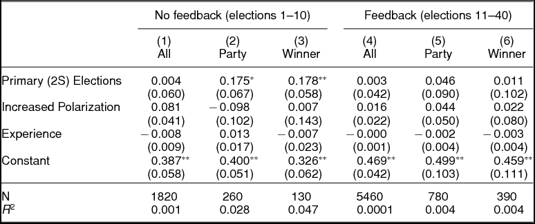
Table 1 presents a series of ordinary least squares regressions to measure the effect of primaries on candidate divergence while controlling for feedback and experience.Footnote 23 The estimates generally reinforce the visual interpretation of the data displayed in Figure 4. Positions diverge (as measured by the intercept) and do not change over time (as the coefficients on Experience are small and insignificant across the models). Although primary elections have no effect on the positions chosen by all candidates (column 1), they do have a statistically significant effect on the divergence between party candidates (those standing for election in the second voting stage, column 2) in the absence of feedback. In 1S elections, the divergence of party candidates from the median voter is 0.4 on the normalized scale (i.e., 40% of the distance between the median and the party ideal point) and increases by a fairly substantial 0.175 in 2S elections (to 57.5% of the distance between the median and party ideal point). The natural consequence of this divergence in party candidates is that election outcomes are more extreme in 2S elections than in 1S elections (column 3).
Regression Analysis of Candidate Positions

* p < .05 ** p < .01, OLS regressions with robust standard errors in parentheses, clustered by subjects in (1), (4) and sessions in (2), (3), (5), and (6).
The effect of primary elections disappears, however, when feedback is introduced, as none of the treatment effects in columns (4), (5), or (6) are statistically significant. Comparing the intercepts with and without feedback suggests that this is because candidates in 1S elections take more extreme positions once feedback is introduced.Footnote 24 Indeed, in 1S elections the average party candidate’s position is 0.400 without feedback and increases to 0.469 in elections with feedback. In 2S elections, feedback appears to have the opposite effect with average positions starting at 0.575 without feedback and decreasing to 0.545 with feedback. The effect of primaries on party candidate divergence thus disappears as the result of countervailing effects of feedback across institutions.Footnote 25
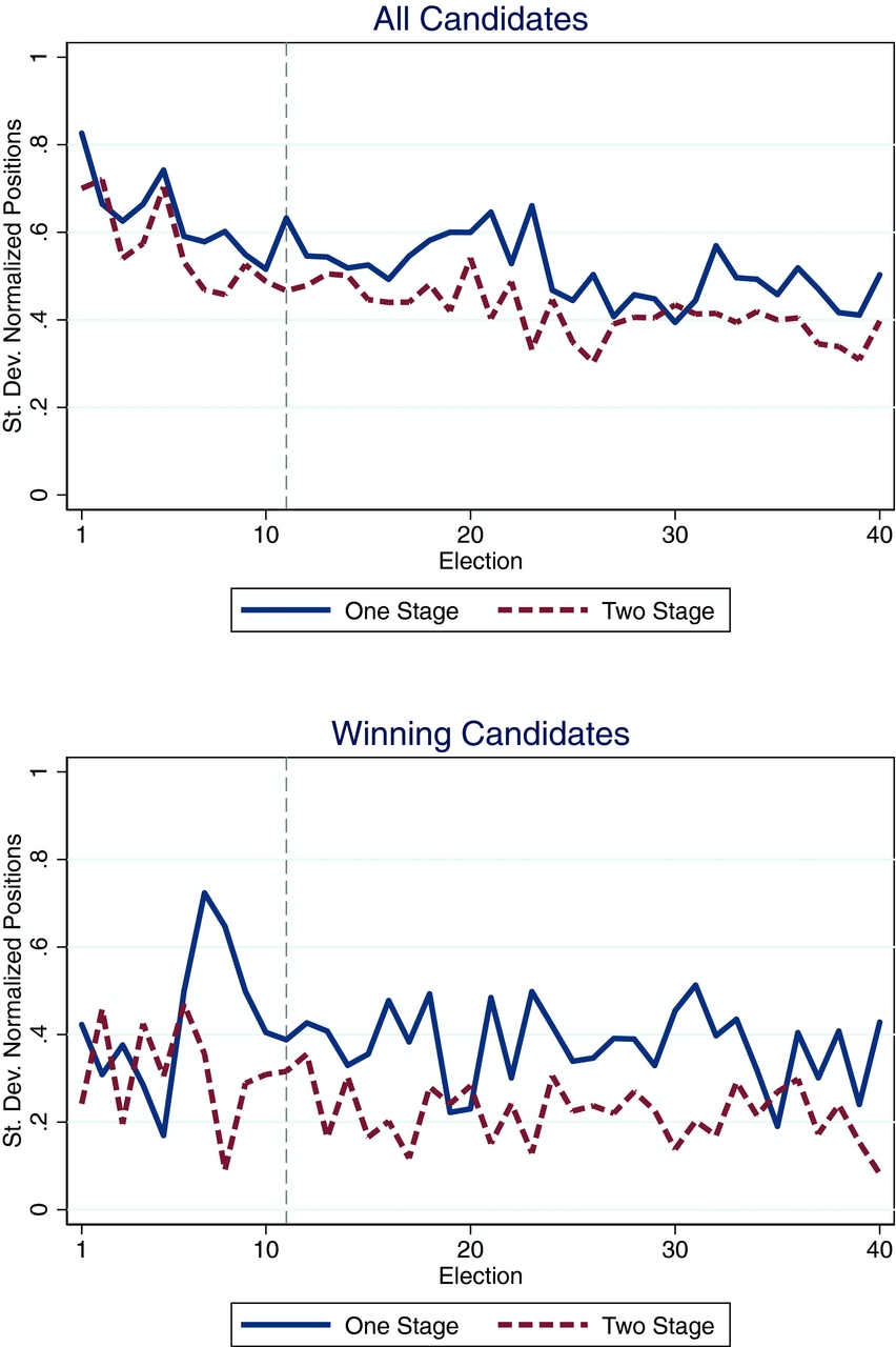
Looking only at average positions obscures the effects of primary elections on other characteristics of the distribution of candidate positions. Although the effect of primaries on average positions is limited to elections without feedback, I find that primaries cause candidate positions to become more tightly centered around the mean—that is, less dispersed. Figure 5 plots the standard deviation of candidate and winning positions over the course of the experiment. The graphs reveal two interesting patterns in candidate dispersion. First, in the upper plot, we see dispersion decreasing steadily over time for all candidates. This implies that because average positions remain unchanged, positions converge, not to the median voter’s position but to the mean position in both 1S and 2S elections. Second, we observe a clear effect of primary elections on dispersion. Variation in positions is consistently lower in 2S elections than in 1S elections for all candidates (upper plot) as well as for winning candidates (lower plot).Footnote 26 Primary elections therefore appear to reinforce candidate polarization by reducing intraparty heterogeneity.
Dispersion of Positions and Outcomes

Voting Behavior
The sample dynamics and analysis of candidate positions suggest that, rather than causing or increasing candidate divergence, primaries instead help to maintain polarization by playing a role in the selection of candidates, weeding out party candidates who are either too extreme or too moderate. In this section, I examine voting behavior in primaries by assessing the extent to which primary voters prefer moderates or extremists and by determining the behavioral rule that best fits the experimental data.
Voters tend to select the more extreme candidate, but it is not an overwhelming preference. Overall, voters sincerely choose the extremist in 56.7% of the elections in the data. When the moderate candidate’s position is closest to the median voter (between 0 and 0.2 on the normalized scale), voters overwhelmingly choose the extremist (69%), especially when both candidates are close to the median voter (90%). Yet, there is an asymmetry because when the extremist candidate’s position is extreme (when the extremist is closest to the voter’s own ideal point between 0.8 and 1 on the normalized scale), the choice between the moderate and extremist is essentially a coin flip (the extremist wins 51% of the time). The more moderate candidates do best when they locate near the midpoint between their party’s ideal point and the median voter and when the extremist is more extreme, but even then, the moderate does not do much better than a coin flip, winning elections at most 57% of the time (when the moderate is between 0.4 and 0.6 and the extremist is between 0.6 and 0.8).Footnote 27
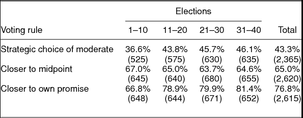
In Table 2, I characterize voting in each set of ten elections according to several possible behavioral rules. The first row shows the percentage of strategic voting for the moderate candidate.Footnote 28 Notice that fewer than half of such votes favor the moderate candidate, 36.6% in the first ten elections without feedback, increasing slightly to 43.8–46.1% in elections with feedback. The slight increase in voting for moderates appears to lend some support for the theoretical framework, as the change in positioning behavior when feedback is introduced is consistent with the change in voting behavior. Without feedback, more votes are cast for extremists than moderates (63.4% versus 36.6%). If candidates expected this, then their best responses would have been to take more extreme positions, which is consistent with the effect of primaries in elections 1–10. When feedback is introduced, there is an uptick in voting for moderate candidates, which would lead candidates to expect less extreme opponents and hence to moderate their own behavior.
Classification of Behavioral Rules for Primary Voting

Total number of votes cast in parentheses, excluding elections where the rule cannot distinguish between candidates.
It is clear, however, that primary voters do not express unconditional preferences for either moderate or extremist candidates in their parties. Table 2 therefore characterizes whether voting is consistent with two additional rules. The second row shows that a simple strategy where voters select the candidate closest to the midpoint between the median voter and their party’s position is a better description of behavior than either strategic or sincere voting. Roughly two-thirds of votes (overall 65.0%) are consistent with this rule, whereas 43.3% of votes are consistent with strategic voting for moderates and 57.7% of votes are consistent with myopically voting for extremists.
The third row of Table 2 suggests that voters behave as if they have heterogeneous “belief-induced ideal points.” This rule appears to be the most consistent with the data.Footnote 29 It assumes that each voter has an individual belief that a candidate located at v*i maximizes their expected utility and therefore votes for the candidate closest to v*i. In the experiment, subjects effectively express such belief-induced ideal points when they choose campaign promises at the beginning of each election, so I use a subject’s campaign promise as a measure of their belief-induced ideal point. Overall, this voting rule attains the highest rate of classification success (76.8%), and outperforms the simple midpoint rule in elections with feedback. By the last ten elections, 81.4% of votes are consistent with voting for the candidate closest to the belief-induced ideal point (one’s own promise earlier in the election), compared to 46.1% strategic voting for moderates, 53.9% sincere voting for extremists, and 64.6% for the midpoint. Because campaign promises and belief-induced ideal points diverge from the median voter’s position, this voting rule has the effect of reducing variance in candidate positions and reinforcing candidate polarization (as discussed in the theoretical analysis and consistent with the patterns shown in the middle triangular distribution in Figure 5).
A Direct Test of Beliefs and Behavior
The experimental finding that candidate positions diverge from the median voter’s position in both 1S and 2S elections supports the behavioral theory predicated on out-of-equilibrium beliefs (Prediction 3) over the competing predictions based on fully strategic candidate behavior with either forward-looking voters (Prediction 1) or myopic voters (Prediction 2). This inference is indirect, however, because beliefs are neither measured nor manipulated in the experiment. To generate a more direct test of the connection between beliefs and behavior, I conducted another version of the experiment in which beliefs are more carefully controlled and manipulated.Footnote 30 In this version of the experiment, subjects play as candidates in the 2S election game. Greater control over beliefs is achieved by having subjects play against computer opponents rather than other subjects. This ensures that the distribution of positions is known and exogenous. Variation in beliefs is induced by providing truthful information about whether the opposing party’s candidate is moderate or extreme.
I conducted three sessions of the modified experiment (54 participants, 18 subjects per session).Footnote 31 Each subject played 20 rounds of the 2S game (with feedback) against computer opponents.Footnote 32 The game was modified so that subjects were informed that the opposing candidate’s position in the general (second stage) election was stochastically determined by a two-part process. First, two opposing primary candidates’ positions were randomly drawn from a uniform distribution over the positions between the median voter’s ideal point and the opposing party’s ideal point. Second, the opposing party’s primary voter (also the computer) randomly selected one of the two positions with equal probability. Information about whether the opposing computer voter chose the moderate or extremist was then provided to the subject. The consequence of this two-part procedure is that candidates faced one of the right-triangular distributions shown in the top right and bottom right of Figure 2. When the opponent was known to be more moderate, the belief distribution should have skewed toward the median voter, and when the opponent was known to be more extreme, the distribution should have skewed toward the opposing party’s ideal point.
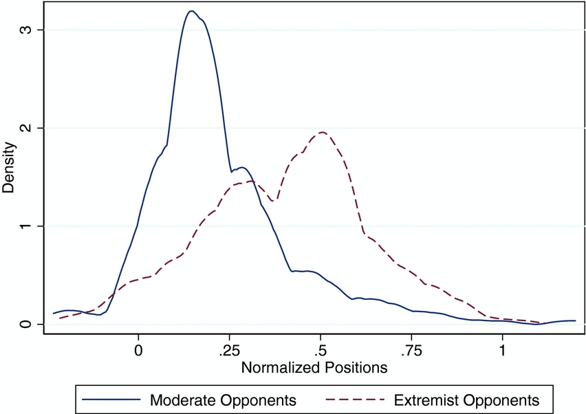
Figure 6 provides a comparison of the distributions that candidates took in response against moderates versus extremists, plotted as kernel densities. The results demonstrate that subjects clearly respond to information about the extremity of their opponents. When computers selected moderate opponents, human candidates took correspondingly moderate positions. Specifically, the majority of such positions (69.6%) fall between 0 and 0.25 on the normalized scale (that is, one-fourth of the distance from the median to their own party’s ideal point). When opponents were extreme, the distribution of positions shifted considerably toward their own party’s ideal point (67.3% of the distribution shifts to above 0.25). In addition, the mode increased sharply, from within the interval between 0 and 0.25 to 0.5 on the normalized scale. On average, positions shifted from 0.20 against moderates to 0.35 against extremists, and this difference is statistically significant (p < 0.01). These results provide direct evidence that candidates’ positions respond to exogenously induced changes in their beliefs, supporting the belief-based behavioral theory.
Candidate Positions against (Computer-Selected) Moderates versus Extremists

CONCLUSION
The theoretical and experimental models I investigate strip away many of the complexities of real-world elections to focus analytically on how introducing primary voters might affect candidate polarization. By drawing on ideas from behavioral game theory and comparing alternative behavioral assumptions, this approach generates new insights about mechanisms that link voter behavior to strategic expectations and, in turn, candidate positioning. Specifically, when candidates and voters have imperfect, out-of-equilibrium beliefs about the behavior of their electoral opponents, the extremity of the positions and candidates they choose depends on their expectations about the extremity of their opponents. Thus, my analysis suggests that the effect of primary elections should be understood to be conditioned by beliefs and strategic expectations and not simply the product of voter preferences.
Experimentally, I find that the need to win a partisan primary does not affect candidates’ positions—candidates’ positions diverge in elections with and without primaries. This is despite a stark setting in which actors are policy-motivated and have complete information. Thus, the experimental evidence lends support to the behavioral theory over more standard analytical approaches to studying strategic interaction that predict candidate divergence. Moreover, candidates are responsive to exogenous manipulations of opposing candidates’ positions, which provides more direct evidence for the mechanism posited by the theory. To the extent there is any polarization, it tends to occur through the behavior of voters rather than the strategic responses of candidates. The effect is relatively small and limited to settings in which participants cannot learn about the behavior of others from past experience.
Interestingly, the experimental data suggest that primaries have an effect, not by increasing candidate divergence, but by increasing the homogeneity of a party’s candidates. Primaries therefore contribute to “ideological purity” in a way that differs from what conventional wisdom would suggest. In the experiment, it is not because primary voters care about ideological purity per se, but because voters use the primary process to weed out candidates both too close to and too far away from the general election median voter’s position. Thus, voters in the lab seem to recognize the tension between centrist policies that yield few policy benefits and extreme positions that are unlikely to win the general election, resolving the tradeoff by generally splitting the difference. Candidates are responsive to this selective weeding out by voters and, as a consequence, take positions that are more homogeneous in elections with primaries than elections without them. This kind of responsiveness likely reinforces polarization in the long-run. Even though moderates are still more likely to win general elections (Hall Reference Hall2015), fewer moderates means that parties and candidates are less likely to learn this from experience, which then inhibits convergence through long-run adaptive electoral processes (e.g., Bendor, Mookherjee, and Ray Reference Bendor, Mookherjee and Ray2006; Kollman, Miller, and Page Reference Kollman, Miller and Page1992).
The behavioral theory helps to make sense of the fact that many people blame partisan primary elections for much of the polarization and dysfunction that afflicts the contemporary American political system but empirical research has not been able to provide compelling evidence to support the claim. For example, the theory is consistent with the findings that neither the introduction of direct primaries (Hirano et al. Reference Hirano, Snyder, Ansolabehere and Hansen2010) nor the format of primary elections (McGhee et al. Reference McGhee, Masket, Shor, Rogers and McCarty2014) has much to do with increasing polarization. It is also consistent with the fact that polarization has been increasing over time despite the absence of significant changes in electoral institutions.
Future observational research should explore the notion that strategic expectations about increasing polarization may be self-fulfilling. For example, the theory implies that partisans who increasingly perceive the opposing party’s candidates to be more extreme will be emboldened to support more extreme candidates of their own. This may explain Bernie Sanders’ popularity in the 2016 Democratic primary and the popularity of other self-proclaimed “Democratic Socialists” in the aftermath of the 2016 elections. With innovative and appropriate measurement techniques, this hypothesis could be tested both cross-sectionally and over time. It is entirely plausible to the extent that citizens infer extreme ideological positions from their dislike of the opposing party (Brady and Sniderman Reference Brady and Sniderman1985), given the steady rise of negative partisanship and affective polarization (Abramowitz and Webster Reference Abramowitz and Webster2016; Iyengar, Sood, and Lelkes Reference Iyengar, Sood and Lelkes2012).
SUPPLEMENTARY MATERIAL
To view supplementary material for this article, please visit https://doi.org/10.1017/S0003055418000515.
Replication files can be found on Dataverse at: https://doi.org/10.7910/DVN/YUNDMQ.





Comments
No Comments have been published for this article.