

Politics is who gets what, when, where, and how.
Harold Lasswell
Introduction
The American states fund myriad policies that impact the lives of their citizens (Morehouse and Jewell, Reference Morehouse and Jewell2004; Boehmke and Skinner, Reference Boehmke and Skinner2012; Gray et al. Reference Gray, Hanson and Kousser2012). Because they operate under strict rules against deficit spending, states are forced to make tough choices across different public policy priorities. If spending on hospitals or highways could be raised without recourse to new taxes or budget cuts elsewhere – if actual spending on public goods were as cheap as talk supporting such spending – there might be little controversy in budget making. But even in political systems where policymakers are able to finance expenditure with new debts, every spending decision bears an opportunity cost and thus invites controversy into the budget process. In short, every year legislators and heads of government in the American states and elsewhere must face trade-offs across budget priorities – trade-offs that we believe form the heart of budget politics.
The aim of this article is twofold. First, we develop intuitions about how ideologically distinct governments set particular spending priorities. These priorities lead governments to increase spending on some items and finance them with relative cuts to spending the opposition prefers. Second, we illustrate the statistical and substantive advantages of treating budgets as the composition of multiple categories. With the exceptions of Philips et al. (Reference Philips, Rutherford and Whitten2016) and Lipsmeyer et al. (forthcoming), whose focus is primarily methodological, we are unaware of any study in the large literature on budgets which uses appropriate methods to examine how increases in one budget area are offset by cuts in others.Footnote 1 Instead, most analysts treat budget categories in isolation, potentially missing the trade-offs which impact every category of public spending. Accordingly, we propose a simple statistical model for time series cross-sectional compositional budget data and use that model to uncover the influence of political and economic variables on spending within, and trade-offs across, all the components of a budget.
The American states present a near-ideal opportunity to examine trade-offs. Compared to national governments, these states operate under hard budget constraints, offer straightforward measures of partisanship, and are data rich. Specifically, we apply our model to annual data from American states over the years 1984–2009, parcelling each annual budget into spending on eight categories: Medicaid and welfare, K-12 education, higher education, highways, public health and hospitals, police and prisons, natural resources and all other spending. Our results show budget categories Democratic and Republican governments favour with extra spending and which parts of the budget they raid to pay for their policy priorities. Democratic priorities include K-12 education and Medicaid and welfare, while Republicans favour highways, police and prisons and higher education. In addition, we uncover how different budgetary rules advantage or disadvantage certain spending items, which policy areas suffer hardest during recessions and which are protected, how states reorder their budget priorities as they grow richer, and how the remaining differences in spending priorities vary across regions of the country once our political and economic variables are taken into account. These findings suggest that trade-offs are an inherent feature of politics that is not exclusive to budgeting in the American states.
An important starting point for our theoretical framework is the assumption that policymakers tasked with creating a budget face a series of pressures and constraints that influence funding priorities. Plainly, policymakers must, at some level, make decisions regarding increases and decreases in public funding. Trade-offs in public budgeting occur when politics and problems disrupt existing modes of expenditure. Policy and public administration scholars have well established that budgetary decisions (like other forms of policymaking) respond to multiple demands from diverse stake holders (Ryu Reference Ryu2015). Some of these demands have priority over others for structural reasons (such as programmatic inertia) or political reasons (such as widely held valence issues, as in Anderson and Harbridge, Reference Anderson and Harbridge2010). We assume that demands on the budget are not only a function of partisan preferences, but also of problems that affect both demands on the budget and its capacity to meet them. While policymaking institutions are built to control the overall size of the budget, individual policymakers often focus on individual programs to provide for constituent demands (Weingast et al. Reference Weingast, Shepsle and Johnsen1981). Thus, an accurate accounting of public budgeting from a policymaking perspective is one that conceives of the budget as composed of bundles of demands rather than as a single aggregate. Competition between particular demands and capacity create trade-offs with notable consequences. Our investigation captures the trade-offs across large categories of policy demands that respond to political demands and financial constraints.
The paper unfolds as follows. First, we review the literature on the political economy of public spending, suggesting a set of covariates likely to shape the trade-offs across budget priorities. We focus in particular on the literature on partisan effects of government spending and derive our expectation that the ideological disposition of government leads to particular spending bundles. In this section, we introduce the idea that partisan governments not only spend on their constituency's demands but simultaneously deny funds to the opposition's priorities. The next section of the paper motivates our focus on the American states and describes the budget data and covariates. We then introduce our method for compositional data analysis and present the results of our analysis. We find that governments led by different parties shift the budget towards preferred areas and away from rival priorities, while institutional, demographic, and especially economic factors have strong budget effects. Finally, we discuss other areas of political science where compositional models might lead to important insights.
Theoretical explanations of budget priorities
The literature on state budget decisions is both vast and deep. One major avenue of inquiry, about which we will say little, focuses on the specific motivations of budgeting officials and the “nuts and bolts” of the budget process (Rubin Reference Rubin1997; Thurmaier and Willoughby Reference Thurmaier and Willoughby2001). Another stream of literature, to which this study contributes, looks instead to the broader political, institutional, and economic forces shaping budgets (Alt and Lowry Reference Alt and Lowry1994; Gilligan and Matsusaka Reference Gilligan and Matsusaka2001; Barrilleaux and Berkman Reference Barrilleaux and Berkman2003; Primo Reference Primo2006; Ryu Reference Ryu2011; Krause and Melusky Reference Krause and Melusky2012; Lewis et al. Reference Lewis, Schneider and Jacoby2015). The best known of these studies examine variation only in the total amount of state spending; however, some works study variation in select spending categories.
We rely heavily on the existing literature for theoretical insights into which political and economic variables are likely to influence the allocation of state spending. Existing literatures rarely or only implicitly discuss trade-offs. Our contribution is to make these statements explicit and to advance a new method for analysing budget compositions. In particular, we identify from this literature three sets of variables – partisanship, budget institutions and economic conditions – which we expect to have systematic effects on the composition of the budget. But even in borrowing from this literature, we face two challenges. First, because our data cover each component of the budget, we must consider many more relationships than a study of a single policy area. Second, because we consider each budget category as part of the whole, rather than as an independent sum of money, some variables commonly employed in studies of spending may have unexpected effects, such as spillovers.
Partisan trade-offs and budget consequences
More than any other political variable, government partisanship features prominently in the discussion of “who gets what” at the state level (Dye Reference Dye1984; Alt and Lowry Reference Alt and Lowry1994; Brown Reference Brown1995; Gilligan and Matsusaka Reference Gilligan and Matsusaka2001). Alt and Lowry (Reference Alt and Lowry1994) and Alt and Lowry (Reference Alt and Lowry2000) show that unified partisan governments – those in which the same party holds the governorship and a majority of House and Senate – are dramatically quicker and better able to adjust state budget outcomes to match their preferences. Dye (Reference Dye1984) and Barrilleaux (Reference Barrilleaux2000) similarly find that democratically controlled legislatures produce polices that are more liberal and more consistent with constituent interests. In particular, Husted and Kenny (Reference Husted and Kenny1997) find that democratic governments generally spend more on welfare programs, consistent with their constituents’ higher demand for redistribution and social insurance.
The literature devotes less attention to the role of parties in other budget areas. The largest portion of state spending goes to education, which is broadly supported by the electorate. This might suggest negligible net partisan effects on education spending as a budget component, but it pays to consider trade-offs within this large category. Ansell (Reference Ansell2010) who notes that education spending provides parties with an opportunity for targeted redistribution, we argue that democratic governments should place relative emphasis on state support for K-12 schools – spending which is disproportionally targeted towards schools in poorer districts – while Republicans should emphasise higher education spending, which lowers tuition costs for students of state colleges, who are more likely to be middle class (Busemeyer Reference Busemeyer2014; Garritzmann Reference Garritzmann2017). Considering other areas of the budget, spending on highways and natural resources benefit suburban and rural voters more than urban constituents, suggesting Republican support may be higher for these areas. Public health and hospitals, on the other hand, seem more likely to be pure public goods and thus less subject to partisan dispute. Finally, over the period studied, Republicans have more often pursued a “law and order” platform, including wider use of mandatory prison sentences, suggesting a higher priority for spending on police and especially prisons, which are typically located in – and provide economic support for – Republican-leaning rural communities (Jacobs and Jackson Reference Jacobs and Jackson2010; Thorpe Reference Thorpe2015).
If Democrats shift state resources towards redistributive programs, and if Republicans shift resources to local public goods targeted at their constituents, those resources will not be available for other state priorities. Focusing on budget compositions brings into sharp relief the notion that parties affect not just levels of particular budgets, but trade-offs among them. Even if a party promises to support all areas of public policy – and, for good measure, to keep taxes low – any effort to raise spending in one area must be complemented with sacrifices elsewhere.Footnote 2 Existing theories of partisan spending largely have neglected this aspect of spending decisions. At best, partisan models of fiscal policy literature only contend that right-leaning governments want a smaller government and left-leaning ones increase the budget.
How parties target those cuts says just as much about their agenda as which budgets they increase. Our expectation is that Republicans and Democrats will raid the preferred policies of their opponents for funds to support their own agendas, while preserving universal public goods from cutbacks. Our argument about raiding opponent’s budget preferences is in stark contrast to theories of partisan competition that focus on issue emphasis (Sigelman and Buell Reference Sigelman and Buell2004; Meguid Reference Meguid2005; Green-Pedersen and Mortensen Reference Green-Pedersen and Mortensen2015). This literature suggests that political parties avoid and deemphasise policy domains where they cannot gain new voters. We go a step further to argue that political parties in power are more confrontational: they intentionally and inevitably deny resources to constituents of the opposition party.
Much of the literature on partisanship in state spending focuses on the question of measurement. Here we follow Alt and Lowry (Reference Alt and Lowry1994) and Alt and Lowry (Reference Alt and Lowry2000) and contrast three types of governments: those in which Democrats have control of the statehouse and majorities in both legislatures, those in which the Republicans have unified control and all other governments, which we term divided. This classification highlights the central importance of the legislative median voters and governor in setting budget policy; moreover, if unified partisan governments fail to differ in policy priorities, it seems unlikely that partisan effects are strong. However, there are other measures of partisan control worth considering. These measures include those which take into account the effects of partisan supermajorities and electoral competitiveness on the parties’ ability to pursue an agenda that benefits their own constituents, rather than one which primarily satisfies the state’s median voter (Barrilleaux et al. Reference Barrilleaux, Holbrook and Langer2002). We leave the investigation of such measures to ensuing work.
Institutional influences
Among the many political institutions influencing the budget process, we focus on two which are highlighted by the public budgeting literature: gubernatorial powers and budgetary rules (Poterba Reference Poterba1996; Ryu Reference Ryu2015).
Gubernatorial powers
Governors draw much of their influence over the budget process from their constitutionally defined authority to set the budget agenda and veto budgets passed by the legislature (Beyle Reference Beyle1996; Barrilleaux and Berkman Reference Barrilleaux and Berkman2003; Kousser and Phillips Reference Kousser and Phillips2012). At one extreme, governors exercise hegemony over the budget agenda, constructing budgets by themselves or with committees appointed at the governor’s discretion. At the other, governors draw up budgets in collaboration with agency officials and legislators not of his or her choosing. Governors’ powers to veto a passed budget also vary, from a simple blanket veto that can be overridden by simple majorities of the legislature, to an item veto, or, in most states, a line-item veto which can be overridden only by a two-thirds legislative majority.
We expect governors to use these powers to advance their budget priorities at the expense of spending in budget categories they either oppose outright or favour less strongly. While we expect individual legislators to prefer spending on local public goods and to participate in log-rolls with other legislators to fund such pork barrel spending, we expect governors, who answer to a statewide constituency, to be less supportive of such funding and more interested in providing statewide public goods (Weingast et al. Reference Weingast, Shepsle and Johnsen1981). Thus under strong governors, we expect spending on highways and natural resources – prototypical local public goods – to shrink. Cutting local public goods provision also gives governors a chance to raise spending on state-wide public goods like public health and hospitals; hence this category should gain under strong governors.
Budget rules
In contrast to the federal government, almost all states are required to maintain a balanced budget in one form or another (Poterba Reference Poterba1996; Fatás and Mihov Reference Fatás and Mihov2006; Rose Reference Rose2008).Footnote 3 As a result, in times of budgetary shortfall politicians should make spending cuts to keep in line with the budgetary restrictions placed on them. Cuts made to satisfy the balanced budget rule need not fall equally across budget categories. We expect entitlement programs, which predominate in the welfare and education categories, to be especially resistant to the budget axe; indeed, automatic increases in entitlement programs may be the key source of budget pressures. Instead, we expect discretionary programs – such as spending on highways, police and prisons, natural resources and the myriad smaller programs lumped in other spending – to bear the brunt of fiscal adjustment.Footnote 4
While most states have strictly balanced budget amendments, some states enjoy a limited ability to deficit spend or carry over past debts. These states should be able to weather budgetary crises with fewer budget cuts and so should reallocate fewer resources from discretionary to entitlement programs. On average, states with strict balanced budget rules should devote a higher proportion of their budgets to entitlements than states with more flexible rules.
Economic factors
The literature on the federal budget suggests economic conditions should have a strong impact on the outcomes of the budget process (e.g. Su et al. Reference Su, Kamlet and Mowery1993). Here, we focus on two commonly examined economic variables: the state unemployment rate and state per capita income.
Unemployment
The unemployment rate provides the clearest available signal of a state’s macroeconomic well-being. Fluctuations in unemployment over the business cycle also trigger automatic spending, especially on welfare programs, and so should strongly impact the proportion of the budget devoted to this area. But state governments must also decide what spending to curtail during a recession, and which budget priorities to protect, even as more resources flow into entitlements.
Real per capita income
If unemployment proxies short-run economic conditions, real per capita income contrasts states at different levels of long-run economic development. Because we are focused not on the size of government but on how relative demand for different types of policy depends on income, it helps to borrow the language of microeconomics, which identifies three ways demand for a good can respond to changes in income. Demand for some goods rises in proportion to income. If everyone, rich or poor, spends roughly the same proportion of their income on a good such as housing, then housing is said to be a normal good. Goods on which the rich spend a greater share of their income than the poor, like international travel, are luxury goods. Finally, inferior goods (or necessities) are those goods, like food, which take up a greater share of the budgets of the poor than the rich.
A long-standing claim (known as Wagner’s Law) holds that economic development is the primary determinant of the size of government. According to the welfare state literature, as an economy grows, government spending will account not only for a growing absolute amount of real dollars but a growing share of the gross domestic product (Wilensky Reference Wilensky1975; Cameron Reference Cameron1978). Because Wagner’s Law focuses on redistributive policy as the main element of the expanding state, we draw from it the hypothesis that welfare spending in particular is a luxury good and should grow as a percentage of the state budget as per capita income rises.
The existence of a luxury good in the state budget – and in a large category of spending – would logically require that some other portions of the budget shrink as income rises. The most likely candidates for inferior goods in the budget are programs favoured by states seeking to develop lagging economies. This could include programs with heavy public investment components, such as highways, natural resources, hospitals and prisons. By the same token, we expect economically developed states to have already made extensive public investments in these areas and better afford to shrink continuing spending in these categories.
Demographic factors
Early work on the growth of the state stressed that slow-moving but long-term demographic changes lead to increasing government commitments. As societies change demands toward the state and, subsequently its reach, increase. Wilensky (Reference Wilensky1975) was among the first to consider structural determinants of government involvement among different spending categories. We follow his lead and consider how two covariates – population density and age composition – result in distinct spending trade-offs.
Population density
How closely people live together within a given boundary affects how governments allocate their funding (Borcherding and Deacon Reference Borcherding and Deacon1972; Bergstrom and Goodman Reference Bergstrom and Goodman1973). Increasing population density might put two forces in motion. A denser population might increase demand for some services to deal with congestion or environmental consequences of density; most notably, these would include mass transit spending, which is grouped in other spending in our rubric, and environmental spending, which falls under natural resources. Other services might see cost savings from physical concentration, particularly for services that can be delivered centrally, such as higher education and hospitals, leading to relative reductions in these spending areas. For most other spending items, the net effect of population density is ambiguous. We therefore expect a null finding on most of them. For example, low density might result more spending on roads as people are spread out over a territory; alternatively, high density may incur in higher costs for traffic control.Footnote 5
Age composition
Different age groups demand distinct types of government support. This demand might be based on two mechanisms. First, the young might simply hold different spending preferences from the old, whereas the elderly may possess more political resources to have their preferences heard. In particular, the welfare state literature shows that preferences for spending across age cohorts are different and the political power of the elderly matters (Pierson, Reference Pierson1995; Busemeyer et al. Reference Busemeyer, Goerres and Weschle2009). Second, spending needs among states might differ depending on the age composition among their inhabitants: this most obviously affects demand for education spending but also should lead to less demand for prisons in states where a higher percentage of the population is too young to serve prison sentences. Both mechanisms point in the same direction. We expect that states with a higher share of young people to spend more on early education and less on prisons, while those with many elderly residents should use their funds for Medicaid and welfare and cut back on both K-12 and higher education. For several other spending categories it is more challenging to make a coherent argument. For example, we believe that age composition is unlikely to affect spending on highways or natural resources.
Data
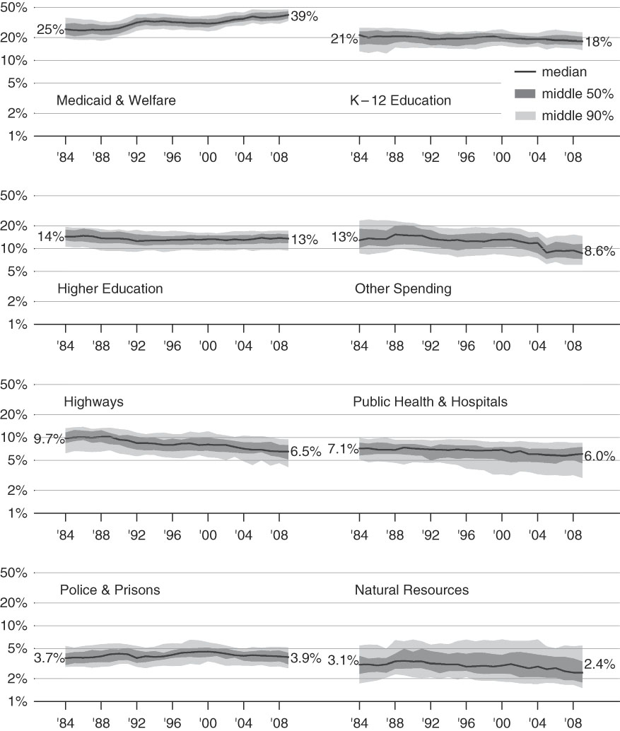
The data we examine comprise yearly state expenditures in eight programmatic categories over 47 states and the years 1984–2009 and are constructed using publicly available data from State Government Finances. We delineate the construction of the eight categories in the appendix.Footnote 6 Our guiding principle is to stay close to actual budget categories but also identify politically relevant groupings. Figure 1 plots the division of the budget across these categories over time for the median state, the middle 50% of states, and the middle 90%. The top three categories of spending – Medicaid and welfare, K-12 education and higher educationFootnote 7 – account for the majority of state budgets: the median state spent 61% of its budget on these categories in 1984, rising to 70% by 2009. Over time, Medicaid and welfare is clearly the fastest growing category of spending across all states, while other spending, highways, public health and hospitals and natural resources all declined significantly as a proportion of their initial budget shares. Spending on education, especially at the K-12 level, lost ground, while the budget share of police and prisons held steady. Although states differ in the shares they devote to each category, the relatively tight 50% and 90% ranges suggest that most state budgets are variations on a common theme. As a result, our task is to illustrate the factors associated with quantitative trade-offs among the categories, rather than to delineate qualitatively different spending regimes.
Temporal and cross-sectional variation in state spending by budget category, 1984–2009. Data from 47 states (excluding AK, HI and NE); Source: U.S. Census, State Government Finances.

We gather covariates from a variety of sources (see Appendix for summary statistics). Most of these data are measured over states and years, though some variables, particularly those measuring institutions, tend to be static in many states. Using data from Hoover and Pecorino (Reference Hoover and Pecorino2005), updated using the Book of States, we identify observations with Unified Democratic Control of the legislature and executive (25% of cases), and those under Unified Republican Control (18%). We measure the stringency of balanced budget requirements across states and years using the American Council on Intergovernmental Relations’ (ACIR) time-invariant 0–10 scale.Footnote 8 Budget Stringency is strongly skewed: most states score the maximum ten points on this scale, indicating the strongest budget rules. Next, we construct an index of Governor Power by summing Beyle’s (Reference Beyle1996, 2003) time-varying 5-point scales of governor’s veto and budget agenda powers.Footnote 9 High scores indicate exclusive gubernatorial control over the proposed budget and restrictions on the legislature’s power to amend the governor’s budget. Finally, we obtain state unemployment rates from the Bureau of Labor Statistics, population density and age composition from the U.S. Census, and per capita state income (in tens of thousands of constant dollars) from the Bureau of Economic Analysis.
Methods
For any government, spending in different policy areas must sum to a constraint, which is simply the overall budget. For the American states – almost all of which are constitutionally compelled to produce a balanced budget – this constraint is binding indeed. Any revision of the budget to expand spending in one area entails an equal and opposite combination of budget cuts and tax increases elsewhere. This linkage across budget areas implies that the political economy of state spending is largely one of trade-offs. However, quantitative analyses of state budgets in political economy generally study budget categories in isolation, or when studying multiple categories at once, implicitly assume independence by estimating separate regressions for each category. These inappropriate models not only make implausible assumptions about the data but also edit out the trade-offs that form the essence of the political process.
Budgets as compositional data
We treat state budgets as compositional data. Denote as
 $$w_{{kit}} $$
the spending in budget category k by state i in year t, where there are K budget categories, I states and T years in total. We normalise all budgets to sum to 1. Our unit of analysis is the collection of budget shares denoted
 $$w_{{kit}} $$
, which for each state and year together fulfil the budget constraint:
 $$w_{{1it}} {\plus} \cdots {\plus}w_{{kit}} {\plus} \cdots {\plus}w_{{Kit}} {\equals}1,\quad \quad 0\leq w_{{kit}} \leq 1$$
Data that obey such constraints are said to be compositional (Aitchison Reference Aitchison1986). With few exceptions, existing work on state budgets ignores the methodological implications of the compositional constraint and in so doing estimates inefficient models with potentially misleading conclusions. It is easiest to see this by considering two commonly employed approaches that fail to take the constraints on
 $$w_{{kit}} $$
into account.
Dangers posed by ignoring the budget constraint in single equation models
Simple linear regression is the most commonly used method for analysing state budget categories, but this model fails because it implicitly makes several assumptions about the compositional nature of budget data. Consider a linear regression model for a single category k=j, so that our response variable is w jit . Linear regression assumes that w jit can potentially take any value from negative to positive infinity. However, for budget data, w jit is bounded by [0, 1] – a state cannot spend negative dollars on a policy, nor can it spend more than its entire budget on any one budget category. Though linear regression will produce unbiased results when applied to bounded continuous data, it will often produce impossible fitted values, suggesting a basic mismatch between data and model.
There is a deeper problem with analysing a budget category outside the context of the complete budget composition. For concreteness, imagine that states can only spend money on welfare, highways, and education, so that the budget for any state and year has three components –
 $$\{ {\rm Welfare}_{{it}} ,\,{\rm Highways}_{{it}} ,\,{\rm Education}_{{it}} \} $$
– which, because of the budget constraint, sum to 1. Suppose that as data analysts we ignore the second and third budget components and fit the following linear regression:
 $${\rm Welfare}_{{it}} {\equals}\alpha _{0} {\plus}\alpha _{1} {\rm Unified}\,{\rm Democratic}\,{\rm Control}_{{i,t{\minus}1}} {\plus}{\epsilon}_{{it}} $$
If we estimate
 $$\hat{\alpha }_{1} \,\gt\,0$$
, we might be tempted to conclude that Democratic governments simply support increased welfare spending. However, substituting from the budget accounting identity,
 $${\rm Welfare}_{{it}} {\equals}1{\minus}({\rm Highways}_{{it}} {\plus}{\rm Education}_{{it}} )$$
, reveals an alternative interpretation of the estimated model:
 $${\rm Highways}_{{it}} {\plus}{\rm Education}_{{it}} {\equals}(1{\minus}\alpha _{0} ){\minus}\alpha _{1} \,{\rm Unified}\,{\rm Democratic}\,{\rm Control}_{{i,t{\minus}1}} {\minus}{\epsilon}_{{it}} $$
Rewritten, the model reveals an alternative interpretation of
 $$\hat{\alpha }_{1} \,\gt\,0$$
: Democrats oppose spending on (the sum of) Education and Highways. These interpretations appear at first to have very different meanings. Both reflect, though neither fully expresses, the finding that Democrats trade-off Welfare spending against Highways and Education. Unfortunately, because we have modelled only a single budget component, we do not know where specifically the budget cuts fall – they could come entirely from Education, entirely from Highways, or from a combination of the two.
Dangers posed by ignoring the budget constraint in multi-equation models
An obvious (but flawed) solution is to run a separate regression for each category. For our three component example, we would estimate three linear regressions:
 $$\eqalignno{ & {\rm Welfare}_{{it}} {\equals}\alpha _{0} {\plus}\alpha _{1} \,{\rm Unified}\,{\rm Democratic}\,{\rm Control}_{{i,t{\minus}1}} {\plus}{\epsilon}_{{it}} \cr & {\rm Education}_{{it}} {\equals}\theta _{0} {\plus}\theta _{1} \,{\rm Unified}\,{\rm Democratic}\,{\rm Control}_{{i,t{\minus}1}} {\plus}\nu _{{it}} \cr & {\rm Highways}_{{it}} {\equals}\lambda _{0} {\plus}\lambda _{1} \,{\rm Unified}\,{\rm Democratic}\,{\rm Control}_{{i,t{\minus}1}} {\plus}\eta _{{it}} $$
Note that this equation-by-equation approach assumes that the components are independent:
 $${\rm corr}({\epsilon}_{{it}} ,\nu _{{it}} ){\equals}{\rm corr}(\nu _{{it}} ,\eta _{{it}} ){\equals}{\rm corr}({\epsilon}_{{it}} ,\eta _{{it}} ){\equals}0$$
. In contrast, the budget constraint requires that if one component goes up, some combination of the others must go down. In general, the components of a budget tend to be negatively correlated, violating the assumption of independence. By ignoring the negative correlations across budget categories, the equation-by-equation approach fails to exploit all of the information in the data and is inefficient (Aitchison Reference Aitchison1986). A model incorporating the information provided by the budget constraint would produce more precise estimates of the quantities of interest and thus a clearer picture of both the factors that influence each budget category and the trade-offs across categories.
The equation-by-equation approach also regularly makes impossible predictions for individual categories and the composition as a whole. Because nothing in the equation-by-equation model constrains the sum of the components to equal the overall budget, the expected budget for any hypothetical values of the covariates will rarely if ever satisfy that constraint. Instead of capturing the actual trade-offs across the budget categories, then, the model often predicts a “budget constraint” that impossibly expands or shrinks to accommodate changes in spending by category. These are not merely methodological quibbles: the inefficiency and impossible predictions of standard models of budgets point to a deep mismatch between the political process that generates budgets and the assumptions of the simple linear regressions commonly used to model them. Trade-offs are the essence of budgetary politics and ignoring them makes neither political nor statistical sense. A covariate can no more affect only a single budget category than a state government can raise spending in one area without taking that money from some other priority.
Estimation and specification
A good model of state budgets jointly estimates the budget categories and respects the unit constraint across them. Fortunately, appropriate models for compositional data are easy to estimate and widely employed throughout statistics, geology and other fields. Surprisingly, although political examples of compositional data are common – including party vote shares in multiparty elections, the proportion of space devoted to particular issues in political speech, and the time budgets of bureaucrats – models of compositional data have received only sporadic attention from political scientists. Recent political science applications of compositional data models include Lantz et al. (Reference Lantz, Alexander, Adolph and Montgomery2014), Adolph (Reference Adolph2013) and Breunig and Busemeyer (Reference Breunig and Busemeyer2012). Philips et al. (Reference Philips, Rutherford and Whitten2016) and Lipsmeyer et al. (forthcoming) add compositional data models and further examples focused on challenges presented by time series data which are nonstationarity and spatial correlated, respectively. Here we focus on a compositional method for stationary time series cross-section data that is easy to implement and interpret – even for many simultaneous components and covariates.
The foundational methods for compositional data analysis are due to Aitchison (Reference Aitchison1986), whose central insight is that while compositional data are jointly dependent and bounded by zero and one, the logarithms of their ratios are independent and unbounded and thus can be jointly modeled using standard multivariate methods for continuous data. Formally, let w it be a K-vector containing the budget shares for a single observation. Then stack all observed compositions into a single IT×K matrix W, which contains one row for each observation and one column for each component. Select one of the columns of W to serve as the reference component. The results do not depend on which column we choose, so for convenience let the last component, K, be the reference. Then apply Aitchison’s additive log ratio transformation to the budget components, which turns the IT×K matrix W into an IT×K−1 matrix Y such that
 $$y_{{kit}} {\equals}\log (w_{{kit}} \,/\,w_{{Kit}} )$$
The columns of Y are independently distributed, yet the new matrix retains all the ratio information in W. This means that the original composition W can be exactly reconstructed from Y, up to the budget constraint. If we estimate a regression model on the log ratio scale, we can easily recover conditional expectations of the original K components for any counterfactual we care to consider (Aitchison Reference Aitchison1986).
Our data have not only compositional but also time series cross-sectional properties. While regression models of compositional time series have received some attention in statistics (Grunwald et al. Reference Grunwald, Raftery and Guttorp1993; Ravishanker et al. Reference Ravishanker, Dey and Iyengar2004; Larrosa Reference Larrosa2005) and political methodology (Brandt et al. Reference Brandt, Monroe and Williams1999), most proposed models are for a single time series and do not easily lend themselves to panel applications (Lipsmeyer et al. forthcoming, is an exception). However, Smith and Brundson (Reference Smith and Brundson1989) show that simple time series models provide consistent estimates of compositions that are invariant to the choice of reference category. If we assume that common dynamic parameters across our units can be pooled, this model easily extends to time series cross-section data.
After transforming the state budget data, we pool the log ratios across time and states and estimate the following K−1 equation time series cross-section compositional data model by seemingly unrelated regressions:
 $$y_{{kit}} {\equals}\mathop{\sum}\limits_{p{\equals}1}^P \phi _{{pk}} y_{{k,i,t{\minus}p}} {\plus}{\bf x}_{{i,t{\minus}1}} \beta _{k} {\plus}\psi _{i} {\plus}t\tau {\plus}{\epsilon}_{{kit}} $$
For each log ratio y
kit
, we specify an equation regressing y
kit
on one or more of its lagged values, as well as a vector of lagged covariates
 $${\bf x}_{{i,t{\minus}1}} $$
, a set of regional dummies
 $$\psi _{i} $$
, and a linear time trend parameterised by
 $$\tau $$
. We estimate the system of K−1 equations jointly by seemingly unrelated regressions, which allow non-zero correlations across the error terms for a given state and period (Zellner Reference Zellner1962).
Our preferred specificationFootnote 10 regresses seven log ratios, formed from the full eight-part budget composition, on four political variables – Unified Democratic Control, Unified Republican Control, Budget Stringency and Governor Power, each lagged one year – and three economic variables – Unemployment Rate, Income per capita and Population Density, also lagged one year. We also control for the state’s region – Northeast, Midwest, South or West – and a linear time trend to allow for secular changes like the steady rise in the price of medical care over the study period and to avoid confounding with political trends like the shift towards greater Republican control. We experimented with different lag structures for the response variable and found little substantive or statistical difference among models with one, two or three lags. We thus settled on a model with a single lag to minimise loss of data to lagging. Panel unit root tests (Im et al. Reference Im, Pesaran and Shin2003) easily rejected the presence of a unit root, confirming our budget log ratios are stationary time series, which allows us to use simpler methods compared to those of Philips et al. (Reference Philips, Rutherford and Whitten2016) and Lipsmeyer et al. (forthcoming). As is typical for time series models of budget data, the model fits the data well, and R 2 for the system of equations was 0.922. There are no missing data.
However, there are several potential sources of bias to bear in mind as we report our results. First, because some of our variables are time invariant (budget stringency, and in some states, partisan control), we could not estimate a model with state fixed effects. Thus there is a danger that our results reflect or are biased by omitted features of states, whether institutional, demographic, geographic or cultural. Including regional effects mitigates but does not eliminate this threat.
Second, budgets not only react to political economic variables but influence them as well. Voters may choose parties in response to existing budget allocations. Governments may change institutions with the aim of reshaping existing budget priorities. And the spending priorities of the government may influence either long- or short-run economic growth. Endogeneity is thus another potential source of bias, but here there are mitigating factors as well. Economic measures such as state unemployment reflect both state-level and national economic conditions, and the latter are not under the state’s influence. By lagging our partisan variables one year to reflect the budget process, we also reduce the risk of conflating political effects on the budget with voters’ reactions to the budget. On the other hand, institutional variables pose perhaps the greatest risk of reverse causation or spurious correlation, as both they and the budget are slow to change and are under the influence of the same political actors.
Interpretation and presentation
Our presentation of results focuses on the reallocation among all budget categories expected when one of the covariates changes. To show these trade-offs clearly, we must translate estimates from the scale of estimation back to the scale of the budget shares and account for the dynamic process by which changes in our covariates influence sticky budgets over a period of years. We must also face the challenge of collating and comparing results across time and across potentially large number of budget categories, which is only possible through carefully designed counterfactuals and visual displays. For each counterfactual, we hold the remaining covariates at their means.
Translating estimates back to budget shares
Because they relate directly to the log ratios of components, and only indirectly to the underlying budget categories, the parameters of an additive log ratio model do not allow easy interpretation in the manner of some linear regression coefficients. However, the estimated parameters
 $$\hat{\phi }_{k} $$
,
 $$\hat{\beta }_{k} $$
,
 $$\hat{\psi }_{k} $$
and
 $$\hat{\tau }_{k} $$
allow us to calculate the expected log ratios
 $$\hat{y}_{{kit}} $$
for any observed or hypothetical values of the covariates. We can easily translate these fitted log ratios back to the composition space by inverting the log ratio, which lets us present the expected budget allocation under the model for any particular scenario of interest.Footnote
11
Accounting for time
The effects of our covariates on the composition of the budget accumulate slowly over time due to the presence of a lagged dependent variable and incremental changes in budgets. Using the impulse-response function enables us to explore the response of the composition over time to changes in individual covariates. However, given the large number of components and covariates in our model, plotting and describing each complete impulse response function is impractical. Instead, we summarise the results by calculating the response in each budget category for the fourth year after a permanent change in each covariate (the choice of period is necessarily arbitrary; we choose four years to focus on the duration of a single gubernatorial term). We also present 95% confidence intervals for these quantities, obtained by stochastic simulation of the iterated response variable (Adolph Reference Adolph2013). To clarify the effect of a given covariate h on a budget category k, we simulate the expected share of the budget category after four years if the value of covariate h changes from an initial value, h
0 (usually its mean) to a new value
 $$h'$$
; this yields
 $${\rm E}(k\!\mid\!h')$$
. We also simulate the expected share of the budget category assuming the covariate stays unchanged at h
0, which yields
 $${\rm E}(k\!\mid\!h_{0} )$$
. We then express the ratio of these two expectations as a percentage change, which reveals how much budget category k would increase or decrease given a change in covariate h, relative to the initial expectation of spending in that category. This allows us to describe a budget area that shifts from 20% of all state spending to 22% as having increased by 10% of its initial level, rather than 2% of the overall budget. Presenting changes in this format helps avoid conflating the size of political and economic effects with the widely different average shares states tend to devote to different budget categories.Footnote
12
Results
Table A3 in the Appendix collects the estimated parameters from our preferred specification for the full compositional data model, which jointly estimates the effects of all our covariates on each budget category using additive log ratio transformations to account for the budget constraint. Because direct interpretation on the log ratio scale is difficult, we focus our discussion of results on simulation showing the shift over time in each budget category as a response to changes in each covariate. Although all results are jointly estimated, we discuss our findings for each category of explanation – partisan control, institutions, economic shocks and demographic change – one at a time. The Appendix also collects discussion of estimated regional differences in our baseline model and full details on alternative specifications, including models dropping budget stringency as a control or adding the growth in the total size of the budget in constant dollars per capita; both alternative models yield substantively and statistically similar results.
Partisan effects
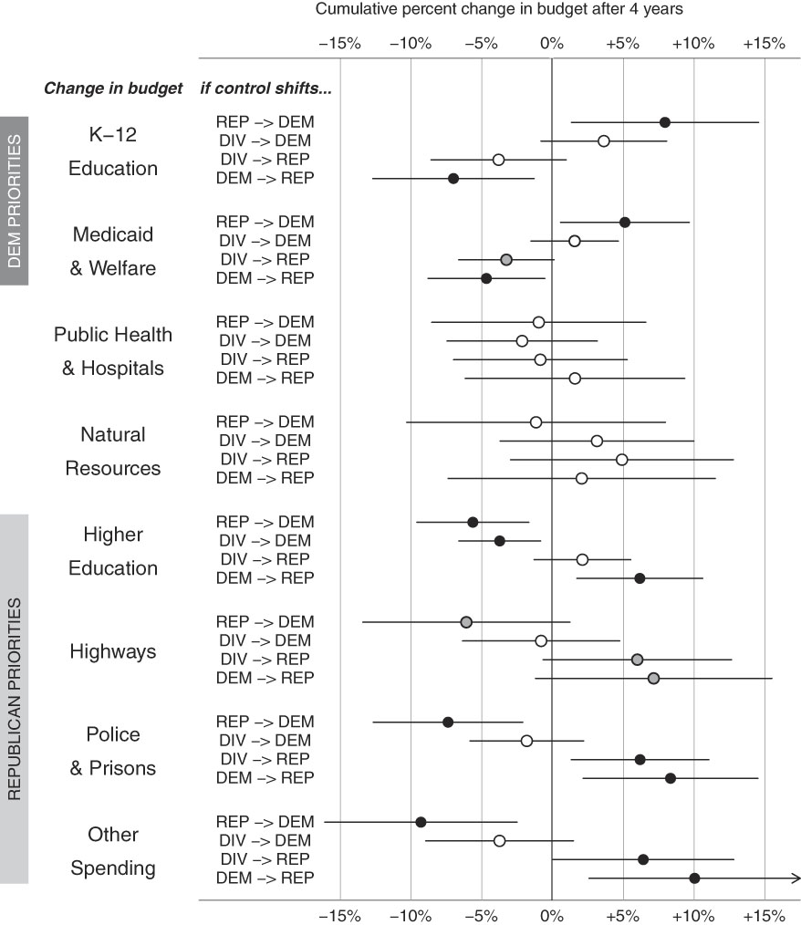
Democrats and Republicans appear to set distinct budget priorities when they hold majorities in both legislative chambers and control the statehouse (Figure 2), including at least five statistically significant effects. Four years after a shift from unified Republican to unified Democratic control, spending on K-12 education increases 7.8% (95% CI: 1.3–14.5%) and Medicaid and welfare increases by 5.0% (95% CI: 0.5–9.7%). A shift in the other direction, to unified Republican control, leads to a 10.6% increase other spending (95% CI: 2.4–19.2%), an 8.2% increase in police and prisons budgets (95% CI: 2.1–14.5%) and 6.1% more state money for higher education (95% CI: 1.7–10.6%). Highways spending also rises 6.9%, though this result is only significant at the 0.1 level (95% CI: −1.2% to +15.5%). Intermediate shifts, such as from divided government to unified control, produce intermediate effects that are often statistically significant.Footnote 13
Estimated change in each budget component four years after a shift in partisan control. Plotted points show the cumulative percent changes in each budget share four years after partisan control of government shifts in the direction indicated. Filled black circles indicate changes that are significant at the 0.05 level, filled grey circles indicate significance at the 0.1 level, and open circles are non-significant results. Horizontal lines are 95% confidence intervals. All results simulated from the model presented in Table A3; all other covariates are held constant at their means.

Both parties find ways to funnel a greater share of state resources to their constituents, with Democrats spending more on social welfare programs and state aid to schools to benefit lower income citizens, and the Republicans shifting those resources into investment in prisons, higher education and (possibly) highways – transfers to the rural, suburban, and middle-class base of the GOP. By focusing on the composition of the whole budget, rather than on isolated categories, we see not only what the parties devote resources to, but also the trade-offs they are willing to make, and those they are unwilling to consider. Relative to Republicans, Democrats’ preference for redistributive spending like Medicaid, welfare and state aid for K-12 education leads them to cut resources that would otherwise flow to some areas Democrats support but do not prioritize, like higher education. Neither party seems willing to pillage more broadly beneficial public goods like public health and hospitals to finance their priorities. The substantive importance of these effects is underlined both by the frequency of shifts in partisan control in the U.S. states – over the period studied, 96% of states had some change in the category of party control and 31% managed to shift from unified control by one party to unified control by the other – and by the fact that regular elections enable contestation over different partisan budget priorities in every election, whether or not voters ultimately opt for change.
Institutional effects
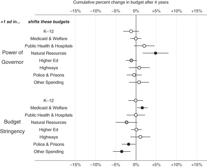
We turn now to the relationship between political institutions and budget priorities (Figure 3). States that raise their governors’ budget and veto powers by one standard deviation at the start of a governor’s term can expect, all else equal, to see natural resources spending to rise 4.8% (95% CI: 1.7–8.0%) and higher education spending to fall 1.2% (95% CI: +0.2% to −2.5%) by the end of her four-year term, though the latter effect is only significant at the 0.1 level. In terms of our theoretical expectations, these results are mixed: there is a hint that institutionally powerful governors increase spending on broadly beneficial public goods like public health and hospitals, but this result is not statistically significant. Meanwhile, powerful governors expand spending on natural resources and have no effect on highways spending, the local public goods we expected them to curtail. The possibility of lower spending on higher education under strong governors is intriguing, as state universities do tend to represent concentrated local public goods for college towns.
Estimated change in each budget component four years after institutional change. Plotted points show the cumulative percent change in each budget share four years after either governor powers or budget stringency increases by one standard deviation from the mean level across states. See Figure 2 for further details.
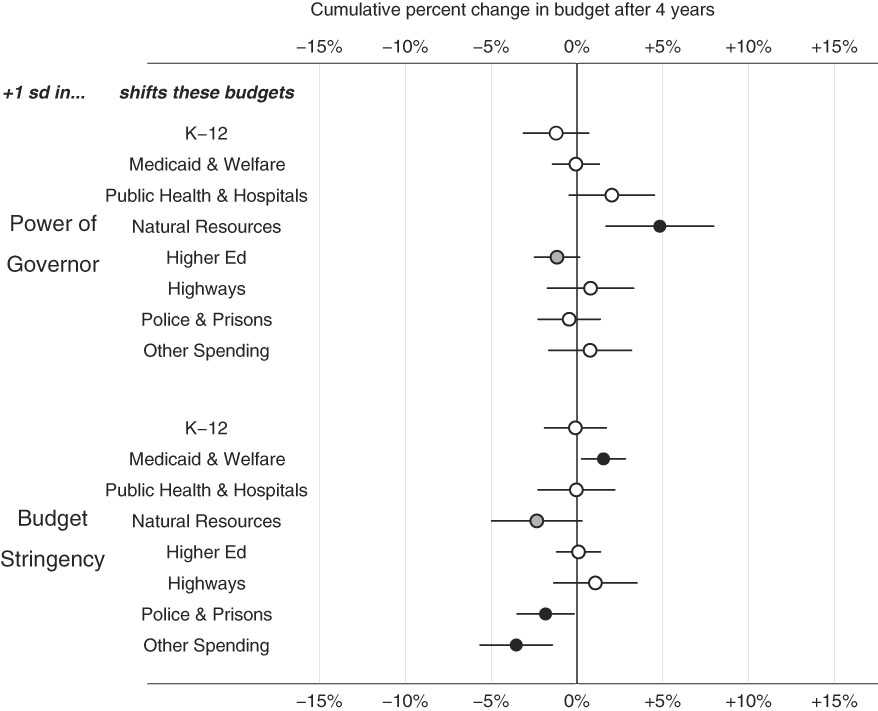
Next we consider budget stringency, which we expected to protect entitlement spending at the expense of discretionary programs. The results here are clearer: four years after increasing budget stringency by 1 standard deviation from its already-high mean, Medicaid and welfare spending is 1.5% higher (95% CI: 0.3–2.8%) while other spending – a catch-all of mostly discretionary programs – falls 3.6% (95% CI: −1.4% to −5.6%), police and prisons’ share drops 1.8% (95% CI: −0.2 to −3.5%), and natural resources declines by 2.4% (significant only at the 0.1 level). Discretionary but arguably more essential programs in the category of public health and hospitals remain unchanged. Interestingly, we did not obtain significant results for the classic discretionary category of highways spending.
Economic effects
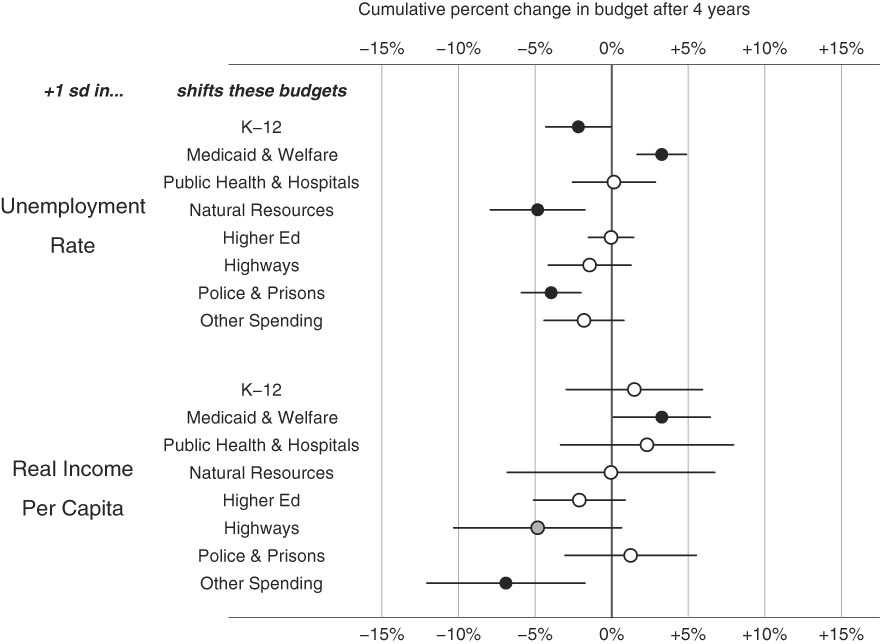
Economic conditions strongly shape budget priorities as well (Figure 4). When unemployment rises by one standard deviation (approximately two points), state budget priorities shift dramatically. Medicaid and welfare’s already large budget share rises by 3.3% (95% CI: 1.7–4.9%), two-thirds the size of the shift associated with partisan control. But unlike parties, who appear to offset increases in spending in favoured areas with targeted cuts in less favoured categories, rising unemployment is accompanied by largely indiscriminant discretionary budget belt-tightening, with significant cuts to natural resources (−4.9%; 95% CI: −1.8% to −7.9%), police and prisons (−4.0%; 95% CI: −2.0% to −5.9%) and K-12 education (−2.2%; 95% CI: −0.1% to −4.3%).
Estimated change in each budget component four years after a permanent economic shock. Plotted points show the cumulative percent change in each budget share four years after either unemployment or real income per capita increases by one standard deviation from the mean level across states. See Figure 2 for further details.
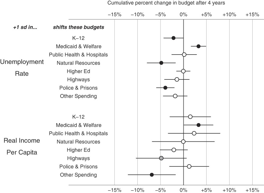
If unemployment lets us examine states’ responses to short-run economic crises, real personal income per capita offers a window into how state budget priorities react to long-term economic development. Following Wagner’s Law, we expect states to increase spending on welfare state programs as they grow richer, while states lagging in economic development should seek to stimulate economic growth through higher spending on public infrastructure and investment. Our results bear out this intuition. According to the model, if we raise personal income by one standard deviation, after five years, Medicaid and welfare spending rises 3.2% (95% CI: 0.2–6.4%), marking welfare spending as a “luxury good.” At the same time, rich states seem to cut back on investment in highways (−4.9%, significant at the 0.1 level), suggesting this category is an inferior good or necessity. The catch-all category of other spending also falls significantly as income rises (−7.0%; 95% CI: −1.7% to −12.0%).
Demographic effects
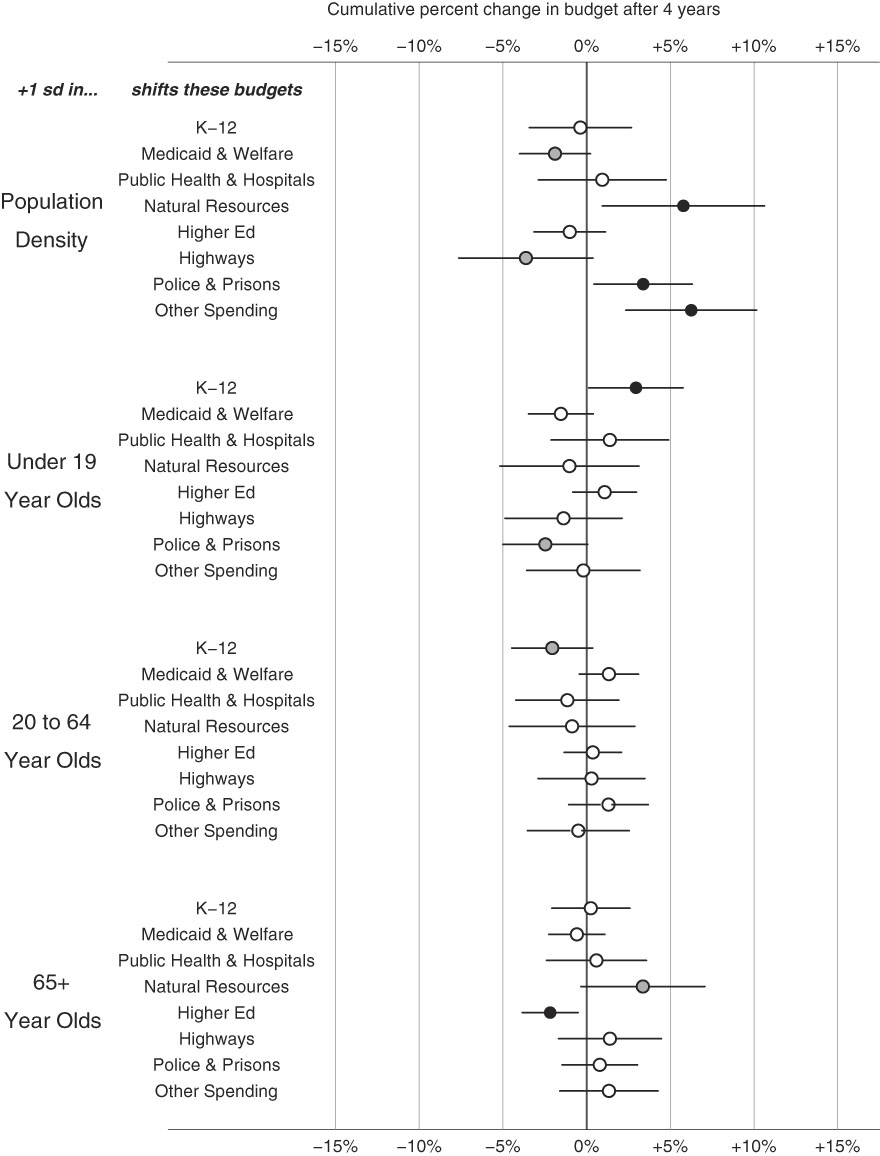
Our final pair of counterfactuals considers how state budget priorities shift with changes in the population (Figure 5). The model suggests several systematic relationships between population density and budget priorities, which generally accord with the different demands of cities: a one standard deviation increase in population density is associated with a 6.2% increase (95% CI: 2.3–10.1%) in other spending, which notably includes mass transit subsidies; conversely, spending on Highways is 3.7% lower (significant only at the 0.1 level). Spending on police and prisons is also higher in denser states (3.3%; 95% CI: 0.4–6.3%), while spending on Medicaid and welfare may be slightly lower (−1.9%; significant at the 0.1 level). Less intuitively, states with denser populations seem to spend 5.7% more on natural resources (95% CI: 1.0–10.6%).
Estimated change in each budget component four years after demographic change. Plotted points show the cumulative percent change in each budget share four years after either population density or one of three age groups increases by one standard deviation from the mean level across states. See Figure 2 for further details.
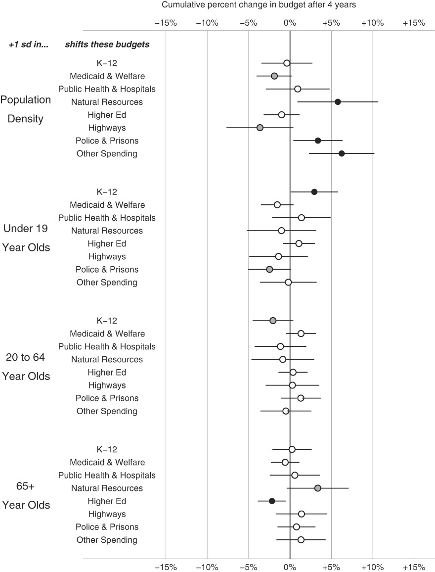
The age composition of the population has few systematic effects, but those present are intuitive: a one standard deviation increase in the share of the population under 19 years of age is associated with spending 2.9% more on K-12 education (95% CI: 0.1–5.8%) and 2.3% less on police and prisons (significant at the 0.1 level); these shifts reflect changes in the share of the population eligible for enrolment or imprisonment, respectively.Footnote 14 Likewise, states with relatively more working-age adults (and thus relatively fewer children and elderly) appear to spend less on K-12 education, though this result is only significant at the 0.1 level. Finally, when the state has one standard deviation higher than average elderly population, higher education spending falls by 2.2% (95% CI: −0.5% to −3.8%). An older population has fewer adults of university age and fewer parents of university-age children, suggesting a similar demand effect; more speculatively, it is worth noting that during the period studied, elderly Americans came from earlier generations with much lower levels of college attainment and thus less personal connection to college as a state budget priority.
Conclusions
While the compositional data approach offers improvements in estimation efficiency and in the sensible prediction of budget shares by category when compared to single-equation models of budget categories, the main payoff from our methodology is that we can provide a clearer picture on the forces that are at play when budgeting is made. These insights complement studies of the size of government and directly improve on isolated studies of single categories. And though our empirical work here is exploratory and our model specification tentative, the budget trade-offs associated with many of our covariates appear both substantively important and theoretically interesting. Two determinants are worth highlighting.
First, we find that partisan governments not only fund policy areas dear to their constituents but also pay for those priorities with targeted cuts to areas less important to the party’s agenda and electoral prospects. To our knowledge, the partisan literature – with the partial exception of recent work on education policy – fails to highlight this aspect of government spending: partisan governments can punish the opposition by reducing spending on opposition items. The combination of increases for the winner and cuts for the loser raises the stakes in budget battles and starkly reveals substantive differences between political parties.
Second, economic downturns have broad effects on the budget. Most areas of policy give up relative resources to pay for increases in welfare spending, with only public health and hospitals, higher education, and to a lesser extent the stimulative category of highways standing immune, at least before the Great Recession. Our results also suggest that as states grow richer, their priorities shift from policies that invest in the state economy towards welfare state programs.
Although we find some effects on budget priorities of budget institutions deemed critical by the literature, the magnitude of these relationships for the most part falls short of the impact of partisanship or economic shocks. We find hints that states under different budgetary institutions allocate resources differently across entitlements and discretionary programs. Budget stringency may protect entitlements at the expense of discretionary spending, and powerful governors may indeed favour some categories over others. But these effects are fairly small. Partly, this reflects a lack of variation in these institutions – almost all states have very strict balanced budget requirements and governors with significant power over the budget agenda. Perhaps state institutions are so similar that the variation in their budget priorities usually reduces to a simple mix of political interests and economic forces. Or perhaps institutional tools are not consistently employed. For example, governors rarely use vetos but when they do they prioritise some spending items (Lauth and Reese Reference Lauth and Reese2006). This logic corresponds to our small estimated effects.
Our analysis also speaks to changes in the mix of spending priorities. Welfare, though also an entitlement, appears highly responsive to economic and political conditions. Spending on welfare programs rises in response to unemployment, grows disproportionately as personal income rises, and is sharply affected by the partisanship of government. And because welfare spending is such a large component of the budget, its fluctuations have large countervailing effects on other categories.
Gains in the share of welfare spending often coincide with deep cuts in spending on K-12 education, highways, other spending, natural resources and police and prisons, but the nature of the trade-off between welfare and other areas depends on the cause of the change in welfare spending. Rising welfare spending threatens K-12 budgets when created by poor economic conditions, but not when driven by changes in the partisan control of government. Generally, shifts in a given budget category depend not only on shifts in specific other budget categories but on the determinants of shifts in other categories. This web of interlocking effects requires that a model relating political, economic and institutional covariates to budget trade-offs to understand when those trade-offs work in one direction or another.
In general, we hope compositional models of budget allocations will uncover new insights as their use spreads. We see at least three further ways this model can help us understand budget politics and public policy more broadly. First, while we have divided spending into programmatic categories, other decompositions of the budget may yield interesting complementary results. For example, some of the hypotheses investigated here could be more sharply tested using budget compositions that distinguish capital and non-capital spending, or discretionary and entitlement spending. These distinctions could be drawn within our programmatic categories or even across them. Likewise, studies could take a closer look at the composition of specific budget areas, examining, for instance, how funds are allocated to different types of welfare programs. We can use the same compositional methods to gain insights on the politics and trade-offs within budget areas that we use to understand trade-offs across them.
Second, we can use these methods to understand the setting of political priorities not just in the United States, but across and within other countries. Cross-national applications of compositional data analysis would give greater scope to institutional explanations by dramatically increasing the institutional diversity of the sample. It would also help move the comparative welfare state literature, a close cousin to the budgeting literature, away from studies of aggregate spending, towards an understanding of the varied composition of that spending and what the trade-offs wrung from political conflicts over scarce resources represent.
Finally, compositional models provide powerful tools to study policy processes more broadly. Theories of agenda-setting stress that governments attend to some issues while ignoring others, as a function of institutional structure and finite information processing capacity (Baumgartner and Jones Reference Baumgartner and Jones1993; Kingdon Reference Kingdon1995). Some policy domains are ripe for government action, while other domains are perceived as unimportant and remain dormant. The compositional analysis we present here offers a way for policy scholars to determine which factors shift the finite supply of attention from one domain to another. For example, future work could consider alternative mechanisms of allocating finite decision spaces, including the share of media attention or legislative hearings devoted to different issues. Alternatively, compositional data analysis may help answer how and when policy-making occurs across distinct policy domains. Are trade-offs starker in domains that deal with more problems and fewer policymakers? Does the institutional setting of policymaking influence the composition of items considered on the policy agenda? Our use of compositional methods shows the importance of thinking about the interdependence of decisions in policymaking, but there is much more to be done.
Supplementary material
To view supplementary material for this article, please visit https://doi.org/10.1017/S0143814X18000326.
Data Availability Statement
Replication materials are available at: https://doi.org/10.7910/DVN/RXMV9W.