1. Introduction
Fast-growing economies like India are likely to witness increasing disparity in living standards between rural and urban areas, with a corresponding increase in migration from rural to urban areas. Lewis (Reference Lewis1954), Harris and Todaro (Reference Harris and Todaro1970), Stark (Reference Stark1984) and Lucas (Reference Lucas, Rosenzweig and Stark1997) are among those who have already offered such hypotheses on internal migration. The weather sensitivity of agriculture and the increasing vulnerability of crop yields to both weather extremes and changing weather conditions are likely to further accelerate the rural-to-rural and rural-to-urban migration. Among other factors that are likely to further increase migration from the rural areas to the cities are changing lifestyles, which could add the amenity dimension to the migration of people from harsh climates to controlled environments. Added to these is the well-recognized factor of increased educational attainments, which could also facilitate movements of people depending on network effects and geographical factors.
Against this backdrop, a few broad generalizations about migration in India are worth underscoring (see part A of the online appendix available at http://journals.cambridge.org/EDE for a detailed discussion on migration patterns in India): (a) the absolute number of migrants from rural to urban areas has increased over time; (b) the migration rate (of the male population) has declined over time, even though the growth rate of migrants has not shown a monotonic trend; (c) the emigration rates are extremely low; (d) inter-state movements are relatively low compared to intra-state movements due to sociocultural factors including language; and (e) temporary circular migrationFootnote 1 rates dominate over long-term migration rates (for further information, see Lusome and Bhagat, Reference Lusome and Bhagat2006; Kundu and Sarangi, Reference Kundu and Sarangi2007). In this context it would be interesting, although difficult, to isolate weather-induced migration from all other factors that might influence people's migration decisions in India.
In recent times, weather-induced migration operating through the agriculture channel has begun to acquire importance due to the emerging concern with climate change. For instance, several studies have shown that climate change could have significant adverse impacts on Indian agriculture (Kavi Kumar and Parikh, Reference Kavi Kumar and Parikh2001; Auffhammer et al., Reference Auffhammer, Ramanathan and Vincent2006; Mall et al., Reference Mall, Singh, Gupta, Srinivasan and Rathore2006; World Bank, 2008). The available evidence so far shows a significant drop in the yields of important cereal crops like rice and wheat under various climate change scenarios, the potential impacts of which in turn can trigger the migration of people associated with the agriculture sector.
While in the past researchers have focused on the linkages between weather variability (and climate change) and migration per se (McLeman and Smit, Reference McLeman and Smit2006; Perch-Nielsen et al., Reference Perch-Nielsen, Bättig and Imboden2008; Bardsley and Hugo, Reference Bardsley and Hugo2010; Dallman and Millock, Reference Dallman and Millock2012; Hassani-Mahmooei and Parris, Reference Hassani-Mahmooei and Parris2012), in more recent times there has been increasing attention by Feng et al. (Reference Feng, Krueger and Oppenheimer2010, Reference Feng, Oppenheimer and Schlenker2012), Barbieri et al. (Reference Barbieri, Domingues, Queiroz, Ruiz, Rigotti, Carvalho and Resende2010), Dillon et al. (Reference Dillon, Mueller and Salau2011), Marchiori et al. (Reference Marchiori, Maystadt and Schumacher2012) and Nawrotzki et al. (Reference Nawrotzki, Riosmena and Hunter2013), among others, on the linkages between weather and its variability and migration operating through the agriculture channel and the rural–urban wage differentials.
Acknowledging that migration can occur for several reasons, this paper focuses specifically on weather-induced migration operating through the channel of agricultural yield changes. While studying the three-way linkages between weather, agricultural yield changes and migration, the paper addresses the following issues in the Indian context:
-
(a) What is the evidence of inter-state migration caused by weather-induced agricultural yield changes?
-
(b) How significant is the impact on migration of crop yield changes at the intra-state level? Does such migration depend on the agricultural crop under consideration?
The analysis presented in this paper is based on Indian Census data for the years 1981, 1991 and 2001 and employs 2SLS/LIML estimation for panel data. The rest of the paper is organized as follows: the second section describes the methodology employed and discusses various issues related to the data used. The subsequent section describes the state-level and district-level results in two separate subsections. The last section provides concluding observations and their policy relevance.
2. Data and methodology
2.1. Migration data
As mentioned in the previous section, migration data in India are available from two major secondary sources – the census data collected by the Registrar General of India and the survey data (employment/unemployment surveys or special migration surveys) collected by the National Sample Survey. Given the small sample sizes in survey data, especially at the district level, this study uses census data for the analysis. In both of these secondary sources, however, the information on migrants is recorded at the place of enumeration, thereby including details only on in-migrants, with emigrants out of the country not recorded anywhere.Footnote 2
The origin and destination of migrants is primarily classified based on the two sectors, rural and urban, giving four ‘from–to’ combinations: (i) rural to rural; (ii) rural to urban; (iii) urban to rural; and (iv) urban to urban (see figure A.2 in the online appendix). Each of these streams of migrants can be further classified as inter-state, inter-district and intra-district migrants based on the two tiers of administrative boundaries – states at the sub-national level and districts within each state.
Since it is expected that migration would take place from less productive regions to more productive regions (or more remunerative regions), the identification of the origin and destination regions of migrants becomes essential in order to carry out a study of the impact of agricultural performance (which is in turn affected by weather/climate factors after controlling for other factors) on the mobility of the people. There are some data limitations in this regard. On the one hand, the individuals who move between states (i.e., inter-state migrants) are identified on the basis of both the state of destination as well as the state of origin. On the other hand, in the case of individuals who move within the state, the district of origin is not indicated in the case of inter-district migrants while the place of origin is not specified in the case of intra-district migrants.
At both these levels of regional disaggregation, the migrant data in each census is classified on the basis of (a) duration of stay, i.e., less than one year, between one and four years, between five and nine years, and 10 or more years of stay; (b) reason for migration (available only at the state level and not at the district level), i.e., marriage, place of birth, employment, and others; and (c) sex, i.e., male or female. The present study focuses on 15 major states of India: Andhra Pradesh, Bihar, Gujarat, Haryana, Himachal Pradesh, Karnataka, Kerala, Madhya Pradesh, Maharashtra, Orissa, Punjab, Rajasthan, Tamil Nadu, Uttar Pradesh and West Bengal. It should be noted that the three newly formed states (Jharkhand, Chatthisgarh and Uttaranchal) as per the 2001 census were included within their erstwhile states (Bihar, Madhya Pradesh and Uttar Pradesh, respectively) from which they were carved out.Footnote 3
We describe the structure of state- and district-level data in detail below. In each case, the final analysis uses the migration rate which is defined as the total (out- or in-) migrants as a proportion of the rural population of the respective region.
2.1.1. State level
The inter-state out-migration data is organized in the following manner. We use the out-migration data from the rural areas of any given state to a rural or urban area of another state as reported in the census for the years 1981, 1991 and 2001. Based on the information provided under ‘reason for migration’, we consider for analysis only those groups of migrants who specify their reason for migration as employment or ‘other’. Since it is not clearly specified in the census data what ‘other’ reasons are, we presume that migration could be due to health reasons, disasters, conflicts, education reasons, and associated movement with the head of the household. All these ‘other’ reasons may have similar economic implications to migration due to employment, but migration due to marriage and place of birth is purely based on social considerations. Consequently, we exclude from the analysis migrants whose reason for migration is either marriage or place of birth. Further, it is observed that the economic considerations contribute to about 50–75 per cent of migration among men and women across different states, with the share ranges between 85 and 95 per cent among men alone.
The panel data model is estimated using information on two durations of stay (i.e., one to four years and five to nine years) under each census and across the states (see table B.1 in part B of the online appendix showing the organization of data across the three censuses). There are 90 observations in the database for the 15 major states of India, with two durations of stay specified for each census year. The out-migration rate at state level refers to rural migrants as a proportion of the total rural population of the origin state. The total rural population is the average of the rural population for the period under consideration with annual values for the inter-censal years obtained from the official projections of the mid-year annual populations of the origin state.
2.1.2 District level
As mentioned before, the number of in-migrants to the rural area of a district forms the basis of the district-level analysis. Such in-migrants include migrants who at the place of enumeration would have reported that they came into the district from another state, from another district and from another part of the same district. In the absence of information on reasons for migration at the district level, we carry out the analysis for total migrants and male migrants separately. As explained in the previous subsection, since marriage is cited as the reason for migration mainly by women, focusing on male migrants would essentially capture migration for employment. Given the significant proportion of intra-district in-migrants, we carry out the district-level analysis for three segments of the migrant population – inter-district, intra-district and total in-migrants in a district.
Due to changes in district boundaries across different census years, the comparability of districts across the census becomes complex. Thus, the analysis at the district level is restricted to the census year of 2001 – the most recent one for which migrant information is available. As for state level data, the duration of stay is also provided at the district level. A five to nine year duration of stay would correspond to migrants having arrived between 1992 and 1996, whereas a one to four year stay would correspond to migrants having arrived between 1997 and 2000. With 504 districts spread across the major states of India and two time points, the panel data that we use for the analysis consist of 1,008 observations.
The district-level in-migration rate is defined as the ratio of total migrants into a rural district as a proportion of the rural population of the receiving district. We thus use the mid-year population projection based on district-level decadal growth rates in rural areas to estimate the population for the year 1996, while using the estimates of rural population totals from the census of 2001 for the second period migration rate. Although the migration data is available as a mass (or sum) of all those who arrived between the two end-points during a given period, other variables used in the econometric model (see description below) are available on an annual basis. Hence, we use the averages of these variables based on the years covering the respective periods to maintain compatibility between migration and other variables.
2.2. Rural population
We obtain the rural population across states for the period 1972–2000 from EOPP.Footnote 4 We then average the rural population for different years, corresponding to different durations of stay for the respective states. We use district level census data provided by the Registrar General of India in 2001 to assemble population data. We use the total rural population in 1996 in a district as the numeraire for estimating the migration rate into a district for migrants arriving between 1992 and 1996. For this purpose, we use the inter-censal rural population growth rate for a district between 1991 and 2001 to interpolate for the year 1996. We carry out a similar exercise to estimate the rural male population. For those arriving between 1997 and 2001, we obtain the district-level total rural population and total rural male population directly from the 2001 census in order to calculate the respective in-migration rates within a district.
2.3. Weather data
We estimate the state- and district-level weather data from the gridded data on temperature and precipitation. The gridded data is based on the database recently released by the India Meteorological Department (Rajeevan et al., Reference Rajeevan, Bhate, Kale and Lal2005; Srivastava et al., Reference Srivastava, Rajeevan and Kshirsagar2009). The temperature data is based on gridded daily temperature data for the period 1969–2005 at 1° × 1° lat/lon resolution, whereas the rainfall data is based on gridded daily rainfall data for the period 1951–2003 at 1° × 1° lat/lon resolution. The weather data at the state and district level is generated following the standard surface interpolation approach.Footnote 5 The weather of a district, for instance, is generated through a weighted average of data from all grids within a 100 km radius from the centroid of the district. As a result, no two districts will have the weather data corresponding to any single grid. It may be noted here that, as the administrative boundaries of state/district are clearly identified in terms of latitude and longitude, it is possible to select the grids relevant for each state/district. Thus, there is significant variation in state and district level weather in the data set. It is important to note here that the analysis does not distinguish between rural and urban weather as it is not feasible to identify the grids that exclusively correspond to rural and urban areas, respectively.
Agricultural performance of crops in India depends crucially on the monsoon period (June to September) and the weather that prevails in different phases of crop growth (Krishnamurthy, Reference Krishnamurthy2012; Pattanayak and Kavi Kumar, Reference Pattanayak and Kavi Kumar2014). Thus, it will be appropriate to construct both annual and seasonal weather variables for the analysis. Accordingly, we generate sowing, growing and harvest period temperature (rainfall) for a particular crop by averaging (aggregating) the daily temperatures (rainfall) for the relevant months.
2.4. Agricultural data
We put together data on crop yields for the years 1972–2000 at the state level as reported in the Indiastat portal, which in turn is collated from the data provided by the Ministry of Agriculture, Government of India. We assemble the district-level data on crop yields for the years 1992–2000 from the Indian Harvest database of CMIE, where the crops covered include rice and wheat. We carry out the analysis separately for the two crops for two main reasons. The results from climate change impact studies indicate that the effect of weather/climate variability is different across these two crops (Krishnamurthy, Reference Krishnamurthy2012) since rice cultivation is not only more widespread but is also more labor intensive than wheat cultivation. It is therefore logical to expect larger migration from a region when the rice productivity declines. The drawback of carrying out separate analyses for each crop would be that it does not capture the substitution possibilities that a household may explore between the two crops in an attempt to adjust to the changing weather/climatic conditions.
Besides rice and wheat yields, we also use the per capita net state domestic product from agriculture for each of the states. We take the yearly net state domestic product (with base year 1970–1971) from the Indiastat portal. (See the online appendix, part C, for a summary of the variables, data source with basic definitions as used in the study.)
2.5. Methodology
We base the econometric estimation on the two-equation model specified below (see Feng et al., Reference Feng, Krueger and Oppenheimer2010).
 $$M_{it}= \alpha +\beta Y_{it} + d_{i} + r_{t} + \varepsilon_{it}\comma \;$$
and
 $$Y_{it}= \gamma +\delta {\bi T}_{it} + p_{i} + c_{t}+ \nu_{it} $$
In equations (1) and (2), M it is the out-migration (in-migration) rate from (to) region i at period t; Y it is one of the agriculture variables (wheat yield or rice yield or per capita net state domestic product from agriculture for region i at period t); and T it is the set of weather variables (represented by annual and seasonal temperature and rainfall discussed in the previous section) of region i at period t, which includes linear or quadratic terms in some of these variables. Since the analysis considers five-year durations as a time period, the weather variability is sometimes better captured through measures of dispersion such as standard deviation than the measures of central tendency like the mean. The d i and p i are the coefficients for the regional (fixed) effects; r t and c t are coefficients to capture time (fixed) effects, and epsiv; it and ν it are error terms in equations (1) and (2), respectively. We include the fixed effects to capture the omitted variables that could be correlated with the variables (yield and weather) used in the model.
Equation (1) captures the migration–agriculture linkage while equation (2) assumes yield to be endogenous in (1), thus using weather variables as instruments to correct for the simultaneity bias of the coefficient of yield in (1). The concerned agriculture variable (primarily yield) is tested for endogeneity in (1) using the robust test score of Wooldridge (Reference Wooldridge, Maddala, Phillips and Srinivasan1995) as reported in Stata 11.0. If it is found to be endogenous, then the two equations are estimated simultaneously, using the two-stage least squares (2SLS) and limited information maximum likelihood (LIML) methods with robust standard errors.Footnote 6 If not, the two equations can be estimated separately using the ordinary least squares (OLS) method to assess the effect of weather on agriculture and agriculture on migration. We consider various combinations of weather variables in the yield equation specification, while we base the model selection on best fit statistics.
2.6. Data structure and interpretation of results
It may be relevant for the inter-state analysis to link the poorer agricultural performance (as influenced by weather variables) of a given region with a higher out-migration rate from that region. The direction of influence of change in agricultural performance (affected as it is by weather variables) on ‘in-migration’ into a district, however, is not easy to hypothesize ex ante. As mentioned earlier, the ‘in-migrants’ into a district include three different streams – those who migrate from another state, from another district and from another part of the same district. The interplay between these different streams of in-migrants and the crop under consideration would, therefore, influence the overall sign of the agriculture variable in the migration equation. For instance, one would expect that if agricultural performance in a district deteriorates, there could be more within-district mobility and less inter-district movement. Thus, if separate estimations are carried out using either within-district movement or between-district movement, the sign of the coefficient of the relevant agricultural variable in equation (1) mentioned above would be negative in the former case and positive in the latter case. The crop under consideration – wheat or rice – could also have an influence on which of these movements dominate, given their relative labor intensity and nature of use (staple vs. non-staple).
Two other issues stand out that would have implications for the interpretation of the results from the econometric model. First, what appears to be a flow of people into a given geographical region is actually to be interpreted as a stock of people residing in a particular region after having moved out of another region. So it is quite possible that certain individuals are more mobile than has been captured at the time of enumeration and that this feature may be more prominent among certain streams of migrants. Thus, individuals who undertake shorter and more frequent spells of movement outside their place of enumeration may not be captured by the migration data of the census. In other words, the two-year panel generated using district-level data is likely to have larger measurement bias compared to the state-level panel generated based on three rounds of census. This could be due to the fact that more people move at district level compared to the state level, and accounting for only those who remain in a district in 2001 may exclude some who could have moved during the intermittent years. This bias could be more significant for the in-migration rate for the five to nine year period. Alongside this, the potential mismatch between the district boundaries and gridded weather data may not adequately identify the supply shocks due to weather within a district. This data limitation may also have implications for explaining within-district movement due to weather shocks. Therefore we focus more on inter-district migration when interpreting the results.
A second related issue is that the migration rate within the five-year duration (from each census) can be seen as the annualized value for that period and not an end of the period rate accumulated over the five-year period. Thus, the results are interpreted as the average annual changes in the migration rate for unit changes in agricultural productivity, all else remaining the same.
3. Weather, agriculture and inter-state out-migration
Inter-state out-migration rates from rural areas form a very small proportion of total migration rates. However, differences exist among states with regard both to these rates and their annual temporal variations. Given the relatively small time scales involved, the temporal variation in the weather variables is not substantial but inter-state variations are quite obvious (see figures D.1–D.5 in part D of the online appendix for a graphical representation).
3.1. Per capita net state domestic product of agriculture and out-migration
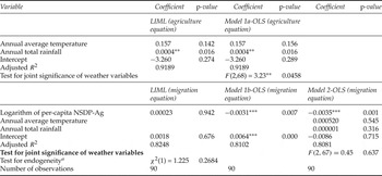
We first analyze the influence of agriculture on migration by estimating the relationship between the per capita net state domestic product in agriculture (henceforth AgInc) and the inter-state out-migration rate with the weather variables as instruments using the approach as outlined in equations (1) and (2) above. The results reported in table 1 show that there is no evidence for endogeneity of per capita net state domestic product in the migration equation. We present the OLS estimates for agriculture and migration equations separately in table 1 (see columns 4 and 5), and for a reduced form equation that describes migration as a function of AgInc and weather variables in columns 6 and 7. We estimate all these equations with fixed effect for time and cross-section (states).Footnote 7
Estimated coefficients for agriculture and migration equations (state-level)

Notes: Agriculture and migration equations use per capita net state domestic product and inter-state out-migration rate as the dependent variables, respectively. Models 1a and 1b, respectively, report OLS estimates for agriculture and migration equations separately; model 2 reports single equation OLS estimates of the migration equation with agriculture and weather variables as regressors. All the models are estimated with fixed effects for time and states although the estimated coefficients are not reported here.
***p ≤ 0.01; **p ≤ 0.05; *p ≤ 0.10. a Test for endogeneity is the Wooldridge's (Reference Wooldridge, Maddala, Phillips and Srinivasan1995) robust score test and the null hypothesis is that the variable(s) are exogenous. The test statistic value and p-value show that the null hypothesis is not rejected.
In the agriculture equation (model 1a in table 1), the weather variables jointly influence the AgInc as seen from the significant value of the F-statistic, while the t-statistic shows that only annual total rainfall influences AgInc after controlling for the other variables. From this model, it can be inferred that AgInc increases with better rainfall. The estimates from the migration equation (model 1b) show that AgInc has a significant negative influence on migration.
Table 1 also reports the estimates of the migration equation with AgInc and weather variables as regressors (see model 2). The estimates show that the weather variables do not influence migration (as observed from the F-statistic for joint significance as well as the t-statistic for individual significance of the weather variables) after controlling for state-level and temporal variations and AgInc. The results further demonstrate that AgInc has a negative and significant impact on the inter-state out-migration rate. The magnitude of impact associated with decrease in AgInc is similar across models 1b and 2.Footnote 8 In other words, the elasticity of the migration rate with respect to AgInc is about −0.775 (when we take the average migration rate across states as 0.004).
Following the climate change and migration literature in the agricultural context (Feng et al., Reference Feng, Krueger and Oppenheimer2010, Reference Feng, Oppenheimer and Schlenker2012), the subsequent analyses focus on the application of the approach outlined in equations (1) and (2) above, keeping crop yields as the potential endogenous variables. Table 2 presents the results for wheat yield and out-migration rates while table 3 gives the results for rice yield and out-migration rates.
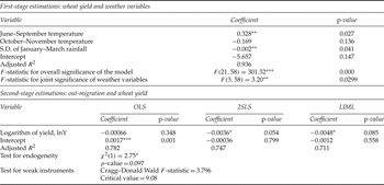
Estimated coefficients for inter-state out-migration: wheat yield and weather

Notes: ***p≤ 0.01; **p≤ 0.05; *p≤ 0.10. Test for endogeneity is the robust score χ 2 test based on Wooldridge (Reference Wooldridge, Maddala, Phillips and Srinivasan1995) with the null hypothesis that the regressor is exogenous. Test for weak instruments is based on Stock and Yogo (Reference Stock, Yogo and Andrews2005) with the null hypothesis that the instruments are weak and the alternative hypothesis is strong. Cragg–Donald Wald F-statistic is obtained from STATA 11.0 using ivreg2 command and the critical value is the 10% maximal IV relative bias also obtained from STATA 11.0.
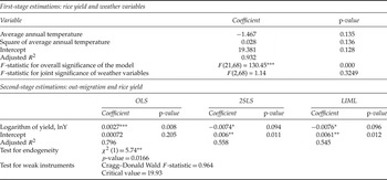
Estimated coefficients for inter-state out-migration: rice yield and weather

Note: As table 2.
3.2. Wheat yield and out-migration
In the agriculture equation, we identify three weather variables – the June–September mean temperature, the October–November mean temperature, and the standard deviation of January–March rainfall – as appropriate instrumentsFootnote 9 after examining several other combinations of temperature and rainfall variables. While the temperature prior to the sowing season (i.e., the June–September temperature) has a positive influence on wheat yield, the increase in growing period temperature (i.e., the October–November temperature) negatively influences the yield after controlling for the effect of other variables. On the other hand, an increase in the variability of rainfall during the harvest period of wheat could adversely affect the yield, all else remaining the same. The robust test score (Wooldridge, Reference Wooldridge, Maddala, Phillips and Srinivasan1995) is significant at 9 per cent, indicating that the wheat yield is endogenous in the migration equation at a higher level of significance. The OLS estimates, however, show that the wheat yield is not significant in the inter-state out-migration equation. Moreover, the test for weak instruments does not reject the null of weak instruments (Stock and Yogo, Reference Stock, Yogo and Andrews2005). Stock and Yogo (Reference Stock, Yogo and Andrews2005) have further suggested that with weak instruments it may be preferable to estimate the coefficients using the LIML method rather than the 2SLS. The LIML estimates are larger in magnitude with a higher p-value when compared to the 2SLS estimates. The elasticity of out-migration to wheat yield change is −1.2.
3.3. Rice yield and out-migration
The results in table 3 for the first equation show that an increase in the average annual temperature has a negative influence on the rice yield while the non-linear effect (captured through the square term) has a positive influence. However, both the variables can be considered to be significant only at the 13–14 per cent level of significance. It is important to note that several other combinations of weather instruments were considered and the reported weather instruments were the ones that are close to 10 per cent level of significance.Footnote 10
As table 3 shows, the robust score test statistic strongly supports the endogeneity of the rice yield in the inter-state out-migration equation, although the weather variables are weak instruments as seen from the corresponding test-statistic value in the same table. The elasticity of out-migration to rice yield change is −1.9 (based on LIML coefficient estimate). The higher value of the elasticity of rice yields compared to wheat yields may be due to the larger number of people involved in rice cultivation than wheat cultivation (as mentioned earlier), which leads to higher mobility when yields decline.
Studies such as Ozden and Swadeh (Reference Ozden, Swadeh and Ghani2010) have argued that inter-state migration in India is influenced by sociocultural factors including language. They have suggested that specific migration corridors exist in India for inter-state movement. Our analysis based on the sub-sample of the states Bihar, Karnataka, Haryana, Madhya Pradesh, Maharashtra, Punjab, West Bengal, Gujarat, Rajasthan and Uttar Pradesh representing the dominant migration corridor when it comes to inter-state movement in India, however, did not provide support for greater elasticity of migration in response to crop yield changes.
In the wheat yield as well as in the rice yield equations, the time dummies are significant and positive for all the years at the 1 per cent level of significance with ‘1972–1976’ as the reference period, indicating that five-year average yields have increased systematically over time after accounting for inter-state variations. Similarly, the state dummies capture the inter-state variations in five-year average yields (after accounting for temporal variations and weather variations across states) with Andhra Pradesh as the reference state. The results indicate that about five of the 14 wheat-growing states and seven of all the states growing rice have significantly different yields, with some lower and some higher than that for the reference state as expected.
4. Weather, agricultural yield and district-level in-migration
Although the results based on the state-level data show indication for the weather–agriculture–migration linkage, the statistical inference does not strongly support it. To increase the variation in the concerned data set, we use a similar analysis using district-level migration information. As mentioned in section 2.1.2, we base the district-level analysis on in-migration from the 2001 census data. As in the case of the state-level analysis, the approach outlined in equations (1) and (2) is adopted with crop (wheat and rice, separately) yields as potential endogenous variables. However, there are a few differences between the state- and district-level analysis as outlined below.
First, since the district-level data do not indicate the reason for migration, we carry out the analysis separately for male migrants and total migrants. Secondly, district-level analysis is not carried out with net district domestic product from agriculture as such data are not readily available in the Indian context for the period of analysis. Alternatively, district-level crop revenue could have been used in place of individual crop yields. Moving away from yield to crop revenue would require consideration of agricultural prices. However, in the Indian context the crop prices (particularly food crops) are not reliable as they are not market determined but are based on state interventions such as minimum support price. Hence there is likely to be less variation across regions brought in by the prices and we expect variation in crop revenue to be not very different from that in crop yields. Therefore, statistically, the results may not be very different between the two variables. Further, anticipating state interventions (on price) to be short term in nature, farmers could rely more on real output changes (i.e., yield) while making decisions regarding migration. This could be even more meaningful in the context of output changes influenced by completely exogenous factors like weather. However, we do acknowledge that if the prices were market determined it would be more appropriate to consider agricultural revenue as it would have removed potential sample selection problems and would have captured substitution among crops.
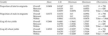
Table 4 gives a summary of the mean and variation in the district-level data.Footnote 11 The district-level analysis has been carried out for three different migrant categories – inter-district, intra-district and total in-migrants in a district. Given that in India districts are fairly large in geographic size with significant variations in agro-climatic conditions as well as infrastructure, it is feasible to expect some climatic conditions (especially, rainfall) to have influence on agricultural performance within a district and hence movement of people. However, it may be noted that it is not easy to establish and interpret a statistical relationship between intra-district movement and intra-district differences in weather.
Mean and standard deviation in select variables across districts and over time

4.1. Wheat yield and in-migration
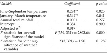
In the wheat yield (agriculture) equation, we identify the three weather variables – the June–September temperature, the January–March temperature, and the annual total rainfall – as the appropriate instruments after considering several combinations of such weather variables available in the database, including the set of instrumental variables used in the state-level analysis. While the pre-sowing (June–September) and harvest (January–March) period temperatures have significant and opposite effects on wheat yield, annual total rainfall has a positive but non-significant influence on the yield (see table 5a).
Estimated coefficients for wheat yield equation with weather variables (first stage) (district level)

Note: As table 2.
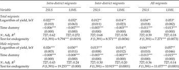
Table 5b reports the estimated coefficient of the wheat yield for intra-district and inter-district migration and all migrants, separately, for total and male migrants. In all the cases the test for endogeneity suggests that the crop yield is endogenous in the migration equation and provides justification for the use of the instrumental variable approach. However, the test for weak instruments shows that the Cragg–Donald Wald F-statistic (3.38) is below the 10 per cent maximal IV relative bias critical value (9.08), indicating that the weather variables are weak instruments and hence the need for interpreting the results cautiously.
Estimated coefficients for in-migration with wheat yield (second stage) (district level)

Notes: The numbers in brackets show p-values: ***p≤ 0.01; **p≤ 0.05; *p≤ 0.10. The time dummy represents the dummy variable for time period 1997–2001 with 1992–1997 as the reference period.
The estimated coefficient of the wheat yield is significant and positive across all the models. The positive sign of the yield coefficient implies that, as the wheat yield decreases, in-migration into that district also decreases. The LIML estimates are uniformly higher than those estimated through the 2SLS approach. The coefficients of the wheat yield in the models involving male migrants are slightly higher than in those involving total migrants. Given the data limitations highlighted in section 2.6, we focus on the results based on inter-district migration rates. The estimated semi-elasticity (based on LIML estimates) of the male (total) migration rate to the wheat yield change is 0.014 (0.014), which suggests that a 10 per cent decrease in wheat yield in a district would decrease the in-migration rate of male (total) migrants by about 0.14 per cent (0.14 per cent).
4.2. Rice yield and in-migration
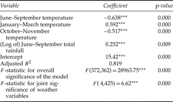
In the model with rice yield as the relevant agricultural variable, four weather variables – three temperature variables and one rainfall variable – are identified as relevant instruments. The three temperature variables are June–September average temperature, January–March average temperature, and October–November average temperature; the rainfall variable is (the logarithm of) the June–September total rainfall. Table 6a reports the estimated coefficients for this first-stage regression. While the increase in pre-sowing temperatures (January–March) is likely to positively influence rice yield, the increase in the southwest/northeast monsoon temperatures (June–September and October–November, respectively) can adversely affect the yield. An increase in the monsoon rainfall also positively influences the rice yield.
Estimated coefficients for rice yield equation with weather variables (first stage) (district level)

Note: As table 2.
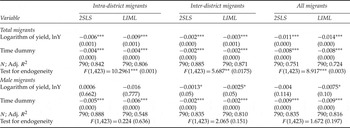
Table 6b reports the estimated coefficients from the second-stage regression for rice. In the case of total migrants, the test for endogeneity indicates that the crop yield is endogenous in the migration equation. The test for endogeneity does not reject the null of yield being exogenous in the male migration rate equation. The test for weak instruments, on the other hand, shows that the Cragg–Donald Wald F-statistic (17.75) is above the 10 per cent maximal IV relative bias critical value (10.27), indicating that the weather variables are not weak instruments.
Estimated coefficients for in-migration with rice yield (second stage) (district level)

Notes: The numbers in brackets show p-values; ***p ≤ 0.01; **p ≤ 0.05; *p ≤ 0.10. The time dummy represents the dummy variable for time period 1997–2001 with 1992–1997 as the reference period.
The estimated coefficient of the rice yield is significant and negative across all models involving total migrants, whereas in the case of male migrants the rice yield coefficient is insignificant for intra-district migrants. As in the case of the wheat crop, we focus on the inter-district migration rate and observe that the estimated semi-elasticity (based on LIML estimates) of male (total) migration rate to rice yield change is −0.0025 (−0.003), which suggests that a 10 per cent increase in rice yield in a district would lead to a decrease in the in-migration rate of male (total) migrants by about 0.025 per cent (0.03 per cent).
The results of district-level analysis significantly differ across choice of crop. The data limitations discussed in section 2.6 could lead to less robust results for the district-level analysis compared to the state-level analysis.
4.3. Hind-casting migration rate
From the estimated model used for migration analysis, one can either forecast or hind-cast the migration rate under various hypothetical changes in the weather variables. The present study prefers to hind-cast, given the likely uncertainties in forecasting based on coefficient estimates sourced from a historical data analysis.
Using the estimations based on the state-level analysis reported in section 3.1, the change in migration rate associated with a 1°C annual temperature change is estimatedFootnote 12 as 0.000413. Since the state-level average annual out-migration rate in the period between 1971 and 2001 was 0.4 per cent, we may conclude that the migration rate during the period would have been 0.44 per cent had the annual temperature been 1°C higher during this period than what it purportedly was according to available records. Similarly, in the case of the wheat crop (section 3.2), the migration rate would have been 0.46 per cent had the October–November temperature been 1°C higher during the 1971–2001 period than what it was.
5. Conclusions
This study sought to explore the linkages between weather, agricultural performance and migration in India using state-level data for the 1981–2001 period and district-level data for the 1991–2000 period. Such a three-way nexus based on a secondary database has not been investigated rigorously in the Indian context and this study fills that gap in the literature. Studies based on migration data in India often focus on the push and pull factors determining migration and are based on single cross-sectional data (e.g., Mitra and Murayama, Reference Mitra and Murayama2008; Joe et al., Reference Joe, Samaiyar and Mishra2009; Ozden and Swadeh, Reference Ozden, Swadeh and Ghani2010). Our study, on the other hand, is based on several years of census data and the movement of people reported within sub-periods of each census, and hence facilitates a rigorous econometric analysis.
The results suggest that, while weather-induced agricultural distress could lead to migration from rural to urban areas in India, the magnitude of the response is relatively small compared to that reported in the literature for developed countries, like emigration from Mexico to the USA and migration within the USA (Feng et al., Reference Feng, Krueger and Oppenheimer2010, Reference Feng, Oppenheimer and Schlenker2012). But the results from this study are comparable to the results reported in other developing countries such as sub-Saharan Africa (Marchiori et al., Reference Marchiori, Maystadt and Schumacher2012). The elasticity of the inter-state out-migration rate with respect to per capita net state domestic agricultural product is approximately −0.775, indicating that a decline in the value of agricultural output related to weather variations results in an increase in the out-migration rate. The crop-wise analysis shows that a 1 per cent decline in rice (wheat) yield leads to a nearly 2 per cent (1 per cent) increase in the rate of out-migration from a state.
The district-level analysis shows larger magnitudes of estimated change in in-migration rates to relative changes in crop yields. However, the district-level analysis provides relatively less robust results compared to the state-level analysis, owing to data limitations that include: (a) larger measurement bias in the migration rate; (b) use of only physical yield and not agricultural revenue as well; and (c) inadequate accounting of supply shocks within a district.
In the absence of other livelihood opportunities in rural as well as urban areas, weather-induced migration operating through the agriculture channel may not lead to significant migration. The low elasticity values reported in this study substantiate this observation. However, the low estimates of elasticity could be due to data limitations emerging from non-accounting of temporary migrants. A recent study by Kavi Kumar and Viswanathan (Reference Kavi Kumar and Viswanathan2013) highlights the differences in the influence of weather variability on temporary migrants as well as permanent migrants using NSS data for India. Although this study does not use agricultural income or yield explicitly in the model, the study results show that migrants involved in agriculture-related activities are usually temporary migrants for whom weather variability (captured by rainfall and temperature) is a major determinant of migration decision. The same study also highlighted the relatively lesser role played by rainfall variability in the decision to migrate permanently.
Further, as noted at the beginning of the paper, the rural-to-urban migrants have registered a larger growth between 1991 and 2001 compared to the previous decade and this is more so in the inter-district and inter-state streams of migration. Thus, one could surmise that, given the current level of development in India, migration is largely explained by the development angle. An even clearer picture would emerge if longitudinal data regarding individual migrants were available at the regional level.
From a climate change perspective, the study findings have important policy implications as migration is often seen as an effective adaptation option by the policy makers. Despite the low magnitude of the impact of crop yield changes on migration rates that this study reports, the presence of linkages between weather, agriculture and migration that it elicits and conclusively establishes here suggests that migration could still be an important adaptation option in India. This is more likely to be the case in the long run given the long time-lags that are typically associated with the manifestation of climate change impacts on people's livelihood options and responses and the likely upward movement of India along the development ladder by that time.