2.1. Model

Before introducing our model, we examine the stability of the relationship between real user cost M4 and real aggregate private investment growth rates over the study period. Figure 2 illustrates the results of the parameter stability test (CUSUM), analyzing the relationship between these variables. The figure clearly reveals that the parameter is not stable over time, with eight structural breaks detected during the entire period. These breaks include three periods with a positive relationship and five periods with a negative relationship between real user cost M4 and real aggregate private investment growth rates.

Given these findings, it is crucial to account for these stylized facts by employing a time-varying parameter FAVAR model for a more accurate estimation. Thus, a time-varying parameters model is justified.

Figure 2.

Stability test on parameter on relationship between user cost M4 growth rate and real aggregate private invest growth rate.

Our model follows Yemba et al. (Reference Yemba, Otunuga, Tang and Biswas2023), as we have observed multiple structural breaks and crises in the U.S. since January 1972 (see Figure 2 above). Given that all series are observable at a monthly frequency after the transformation, the state-space representation of the MF-TVP-FAVAR(p) model can be expressed as follows:

(1) \begin{align}&\qquad\,\,\, X_{t}=\Gamma ^{F}_{t}F_{t}+\Gamma ^{Z}_{t}Z_{t}+v_{t}, v_{t}\sim i.i.d. N(0,R_{t}) \end{align}

(2) \begin{align}& \begin{pmatrix} F_{t}\\ Z_{t}\\ \end{pmatrix} =C_{t}+\sum \limits _{j=1}^{p}B_{t,j} \begin{pmatrix} F_{t-j}\\ Z_{t-j} \end{pmatrix}+e_{t}, e_{t}\sim i.i.d. N(0,Q_{t}), \end{align}

where $\Gamma ^{F}_{t}$ are factor loadings, $\Gamma ^{Z}_{t}$ are regression coefficients, $F_{t}$ is the latent factors that have impact on our variables of interest, but they cannot enter the normal vector $Z_{t}$ of VAR model, $C_{t}$ is the intercept, and $(B_{t,1}, \ldots , B_{p,t})$ are VAR coefficients. $v_{t}$ and $e_{t}$ are zero-mean Gaussian disturbances with time-varying covariances $R_{t}$ and $Q_{t}$ , respectively, and $p$ represents the order of the model. (1) and (2) represent transition equations. We adopt the common identifying assumption in the factor literature that $R_{t}$ is diagonal, thus ensuring that $v_{t}$ is a vector of idiosyncratic shocks and $F_{t}$ contains information common to all latent variables. We assume that US economy is driven by fundamental unobserved factors and the latter can be categorized into activity, prices, financial, and interest rate factors. These factors capture fluctuations of key macroeconomic variables such as output, price, interest rates, and aggregate private investment.

We follow the assumptions proposed in the literature (e.g., Banerjee et al. (Reference Banerjee, Marcellino and Masten2008), Breitung and Eickmeier (Reference Breitung and Eickmeier2011), Bates et al. (Reference Bates, Plagborg-Møller, Stock and Watson2013), Koop and Korobilis (Reference Koop and Korobilis2014)) that emphasize model flexibility by allowing all parameters to vary over time and accounting for structural breaks in factor loadings. These assumptions are particularly important in our context, as we expect time variation and structural breaks in both the loadings and the covariances of factor models that incorporate the growth rate of aggregate private investment alongside a broad set of macroeconomic and financial variables. Moreover, we follow the recent VAR literature that employs heteroskedastic covariance matrices, $R_{t}$ and $Q_{t}$ , which yield more consistent impulse response functions (IRFs) compared to models that assume homoskedasticity (e.g. Koop and Korobilis (Reference Koop and Korobilis2014)).

Similar to Koop and Korobilis (Reference Koop and Korobilis2014) our model employs a multivariate system to estimate the IRFs using all latent factors and macroeconomic variables. Unlike Koop and Korobilis (Reference Koop and Korobilis2014), we do not differentiate between macroeconomic and financial variables. Our latent factors consist of macroeconomic variables from economic activities, prices, and interest rates. Thus, the final estimated factors reflect information associated with divisia and user cost of monetary aggregates.

To complete our MF-TVP-FAVAR model, we define the measurement equations

(3) \begin{align}&\qquad\qquad Y_{t}=M^{y}_{t}\Lambda ^{y}Z_{t}, \\[-7pt] \notag \end{align}

(4) \begin{align}&\qquad\qquad H_{t}=M^{h}_{t}\Lambda ^{h}F_{t}, \\[-7pt] \notag\end{align}

(5) \begin{align}& \Gamma _{t}=\Gamma _{t-1}+u_{t},u_{t}\sim i.i.d. N(0,W_{t}) \\[-7pt] \notag\end{align}

(6) \begin{align}&\, \beta _{t}=\beta _{t-1}+\eta _{t},\eta _{t} \sim i.i.d. N(0,V_{t}) \\[-7pt] \notag\end{align}

where $\Lambda ^{y}$ and $\Lambda ^{h}$ are aggregation matrices based on the weighting scheme underlying latent variables quoted at monthly frequency; $M^{y}_{t}$ and $M^{h}_{t}$ are deterministic selection matrices that yield a time-varying observation vector by selecting rows corresponding to the monthly variables (see Mariano and Murasawa (Reference Mariano and Murasawa2003), Schorfheide and Song (Reference Schorfheide and Song2015), and Ankargren et al. (Reference Ankargren, Unosson and Yang2020)).

To transform the quarterly data to monthly form, we rewrite equation (3) as follows

(7) \begin{eqnarray} Y_{t}= \begin{pmatrix} Y_{mt}\\ Y_{qt} \end{pmatrix} = \begin{pmatrix} I_{n_{m}}&\quad 0 \\ 0 &\quad M^{Y}_{qt} \end{pmatrix} \begin{pmatrix} I_{n_{m}} &\quad 0 \\ 0 &\quad \Lambda ^{Y}_{q} \end{pmatrix} Z_{t}=M^{Y}_{t}\Lambda ^{Y}Z_{t} \end{eqnarray}

where the subscripts $m$ and $q$ denote monthly and quarterly frequency respectively, $Z_{t}=\big(\begin{matrix} Z^{\prime}_{mt},Z^{\prime}_{qt} \end{matrix}\big)' =\big (z^{\prime}_{t}, \ldots , z^{\prime}_{t-p+1} \big )$ , $t=1,\ldots , t_{b}$ , $t_{b}$ denotes the final time period where all the monthly variables are observed. Therefore, when $t\leq t_{b}$ , all monthly series are observed. However, if all the quarterly series are observed at time $t$ , both $M^{y}_{qt}$ and $\Lambda ^{y}_{q}$ are identity matrices of dimension $n_{q}$ so that $Y_{qt}=\big(\begin{matrix} 0&\Lambda _{q} \end{matrix}\big)$ .

For the remaining period (for $t\gt t_{b}$ ), $M_{q}$ is an empty matrix such that $Y_{t}=Y_{mt}$ . In this case, the matrix $\Lambda ^{y}_{q}$ contains scheme of unobserved high-frequency latent observations $Z_{qt}$ into some observed low-frequency observations $Y_{qt}$ .

Following Mariano and Murasawa (Reference Mariano and Murasawa2003) and Dal Bianco et al. (Reference Dal Bianco, Camacho and Quiros2012), we use quarterly difference of $Y_{qt}$ to construct the observed growth rate:

(8) \begin{align} Y_{qt}=Y^{*}_{qt}-Y^{*}_{qt-3}&=\frac {1}{3}\big[(Z^{*}_{qt}-Z^{*}_{qt-3})+(Z^{*}_{qt-1}-Z^{*}_{qt-4})+(Z^{*}_{qt-2}-Z^{*}_{qt-5})\big] \\[3pt] \notag&=\frac {1}{3}\big[\Delta Z^{*}_{qt}+2\Delta Z^{*}_{qt-1}+3\Delta Z^{*}_{qt-2}+2\Delta Z^{*}_{qt-3}+\Delta Z^{*}_{qt-4}\big] \end{align}

where $Y^{*}_{qt}$ denotes the observed quarterly log-level (for $t\leq t_{b}$ ) and the latent variable quarterly log-levels (for $t\gt t_{b}$ ). The latent variable is defined as $Y^{*}_{qt-3}=3\Delta Z^{*}_{qt}$ .

The efficient compact formulation of the state-space model (1) to (6) can be improved by eliminating, for $t=1,\ldots ,t_{b}$ , the monthly observations $Y_{mt}$ from the state vector $Z_{t}$ that appears in the measurement equation (3). Even though the monthly variables are observed for all points of time, there are some observations that are missing at the end of the sample, called as a ragged edge (Banbura et al. Reference Banbura, Giannone, Modugno and Reichlin2013), which generates unbalanced monthly data for $t=t_{b}+1$ . The dimension of the state-space model is reduced from $np$ to $n_{q}(p+1)$ . This treatment is more convenient for handling the factor variables, $F_{t}$ of our FAVAR in equation (4).

Additionally, the model assumes that $u_{t}$ and $\eta _{t}$ are uncorrelated over time and with each other. This assumption is at the core of the definition of the small-scale dynamic factor model as in Stock and Watson (Reference Stock and Watson2009) and implies that the model separates out common correlation underlying the observed variables from individual variations in each series. In vector form, we define $F_{t}= \big(\begin{matrix} F^{\prime}_{mt},F^{\prime}_{qt} \end{matrix}\big)'$ , $\Gamma _{t}=\big(\begin{matrix} (\Gamma ^{F}_{t})^{\prime}, (\Gamma ^{Y}_{t})^{\prime} \end{matrix}\big)$ , and VAR coefficients $\beta _{t}= \big(\begin{matrix} C^{\prime}_{t}, \mbox{vec}(\beta _{t,1})^{\prime}, \ldots , \mbox{vec}(\beta _{t,p})^{\prime} \end{matrix}\big)^{\prime}$ . For simplicity, we assume that the vectors of loadings $\Gamma _{t}$ and VAR coefficients $\beta _{t}$ evolve as multivariate random walks (RW).

The $n \times 1$ vector $Z_{t}$ of macroeconomic variables enter the regular $Z_{t}$ of a VAR model. $Z_{t}$ consists of $n_{m} \times 1$ vector $Z_{mt}$ containing the variables that are observed at monthly frequency and $n_{q}\times 1$ vector $Z_{qt}$ containing the variables that have been observed at quarterly frequency. In vector form, $Z_{t}= \big(\begin{matrix} PFINV_{t}, EMPL_{t}, INFL_{t}, CONCFI_{t}, CP_{t}, BUSL_{t}, UCM4_{t}, UNCERT_{t} \end{matrix}\big)$ where $PFINV_{t}$ , $CP_{t}$ , $BUSL_{t}$ , $EMPL_{t}$ , $INFL_{t}$ , $CONCFI_{t}$ , $UCM4_{t}$ and $UNCERT_{t}$ respectively denote the real aggregate private investment growth Rate ( $PFINV_{t}$ ), real aggregate corporate profits after tax ( $CP_{t}$ ), real total business loans growth rate ( $BUSL_{t}$ ), non-farmers employment growth rate ( $EMPL_{t}$ ), CPI inflation rate ( $INFL_{t}$ ), consumer confidence index ( $CONCFI_{t}$ ), growth rate of M4 user cost ( $UCM4_{t}$ ), and economic uncertainty index ( $UNCERT_{t}$ ) at time $t$ .

The selection of these macroeconomic variables is guided by empirical literature on private investment dynamics (Arif and Lee (Reference Arif and Lee2014); Kopp (Reference Kopp2018); Azzimonti (Reference Azzimonti2018)). Why do we use employment growth instead of real GDP growth? Employment growth captures labor demand, which is directly linked to firm-level investment and hiring decisions. It provides a clearer signal of real economic activity, especially when assessing investment behavior or consumption capacity. For financial variables, our choices are based on theoretical considerations suggesting that loans, bonds, and equity markets are key sources of financing for corporate investment. In the context of bond markets, real corporate profits after tax are included to reflect the supply-side factors affecting bond issuance, such as expected returns and tax considerations. Total business loans are used to capture the bank lending channel. Corporate profits also serve as a proxy for equity market conditions, given their relevance to retained earnings and stock valuations.

Following the critique by Cooley and LeRoy (Reference Cooley and LeRoy1985), different orderings in a Cholesky decomposition imply distinct underlying structures of the economy. To address this, we adopt the ordering framework proposed by Christiano et al. (Reference Christiano, Eichenbaum and Evans2005) for variables in the VAR ( $Z_t$ ). In this framework, macroeconomic variables enter first because they are assumed to be exogenous to firms’ investment decisions. Financial variables follow, as they are considered endogenous to firms’ decision-making processes. This ordering ensures that the VAR model is exactly identified.

We include two key financial variables: real aggregate corporate profits after tax and real total bank loans to businesses. In fact, firms primarily invest to generate profits; therefore, real aggregate corporate profits after tax are placed before real total loans in the VAR. Furthermore, firms’ primary sources of investment funding include loans from financial institutions (e.g., commercial banks) and the issuance of bonds and stocks. To account for the financing side of investment, we include real total business loans. These financial variables, being endogenous in our model, are positioned last (after the variables describing the real activities) in the VAR. We slightly depart from the existing literature that often utilizes the price of financial variables, such as the federal funds rate or monetary aggregates, to describe both financial conditions and monetary policy instruments. Instead, we focus exclusively on indicators that represent the quantity (value) of financial variables.

In addition to these macroeconomic and financial variables, we incorporate a measure of uncertainty to better capture macroeconomic fluctuations, including variations in aggregate private investments. Our approach to measuring macroeconomic uncertainty is consistent with the methodology outlined by Jurado et al. (Reference Jurado, Ludvigson and Ng2015), including their placement of the uncertainty variable as the last entry in the VAR model. Furthermore, our variable of interest, the growth rate of real user cost, is positioned in the model just before the uncertainty measure. To some extent, this variable may serve a role similar to that of a monetary policy instrument. This measure of user cost M4 does not include treasury bills (with maturity equal or less than five years).

We will compare the results of our specification (based on real user cost of M4 monetary aggregates) with an alternative one with a measure of interest rates represented here by spread between the Baa corporate bond yield (Baa) and the 10-year Treasury Bond yield. This comparison is consistent because both indicators capture the spread between the highest yield on a long-run risky asset and the yield of a long-run riskless asset (monetary asset or treasure (bill or bond)). We depart a little bit from Azzimonti (Reference Azzimonti2018) who used Aaa corporate bonds yield as a measure of interest rate because we believe that Moody’s corporate bonds quoted AAA do not represent the majority of bonds. Thus, the alternative model is $Z_{t}= \big(\begin{matrix} PFINV_{t}, EMPL_{t}, INFL_{t}, CONCFI_{t}, CP_{t}, BUSL_{t}, SPREAD_{t}, UNCERT_{t} \end{matrix}\big)$ .

We use a dual conditionally linear Kalman filtering/smoothing algorithm developed by Koop and Korobilis (Reference Koop and Korobilis2014) to estimate our model (1) to (6) by Kalman Filter and smoothers. First of all, we use the approach of Mariano and Murasawa (Reference Mariano and Murasawa2003) and its adaptation in (Schorfheide and Song, Reference Schorfheide and Song2015) described above to modify the state space model (1) - (6). Then, we implement a simplified version of the algorithm developed by Koop and Korobilis (Reference Koop and Korobilis2014) for estimating our MF-TVP-FAVAR model ( $\theta _{t}=(\Gamma _{t}, \beta _{t})$ ). The variance discounting methods combined with the Kalman filter are used to obtain analytically consistent results for the posteriors of the state variable $F_{t}$ and the time-varying parameters $\theta _{t}=(\Gamma _{t}, \beta _{t})$ . The identification of our model proceeds as standard, restricting the variance-covariance matrix $R_{t}$ to be diagonal and applying a Cholesky decomposition with sign restrictions. We impose a negative sign on the parameters capturing the effects of both the credit spread and the real user cost of M4 growth rate shocks on all other variables in the matrix $Z_{t}$ , except for inflation, which typically decreases in response to monetary tightening. To determine the optimal number of lags for our FAVAR model, we employ the Bayesian information criterion (BIC). The BIC results indicate that the optimal lag length for our model is two (2).

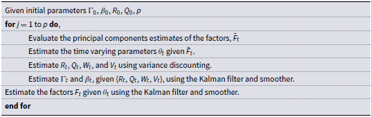
A simplified version of the algorithm developed by Koop and Korobilis (Reference Koop and Korobilis2014) for estimating our MF-TVP-FAVAR model is given in the following steps:

Algorithm 1:

Simulation scheme

We compare our results with those obtained using an alternative ordering, where the uncertainty variable enters last in the macroeconomic variables block. Additionally, we redefine the real user cost M4 to include Treasury bills with maturities of five years or less.

2.2 Data

Our model is estimated using monthly observations from January 1972 to September 2023, covering 120 time series over a half-century period. These series include data from different sources:the Federal Reserve Economic Data (FRED) at the St. Louis Fed, the Board of Governors of the Federal Reserve, the Bureau of Economic Analysis, and the Center for Financial Stability. Some quarterly series are incorporated into the model using the technique described above. All non-stationary variables are transformed into stationary series after first difference. The series used to construct the factors are detailed in the appendix (113 time series).

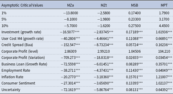
Table 1 presents stationarity tests for our main variables, including the real user cost M4 growth rate (excluding Treasury bills), real aggregate private investment growth rate, credit spread growth rate, real aggregate corporate profits after tax, real aggregate business loan growth rate, employment rate, inflation rate, consumer sentiment index, and economic uncertainty index. The results indicate that all series are stationary except for real aggregate corporate profits after tax, which becomes stationary after first difference.

Table 1.

Unit root tests

Note: These tests are proposed by Ng and Perron (Reference Ng and Perron2001). $^{*}$ , $^{**}$ , and $^{***}$ denote rejection of the unit root null at 10%, 5%, and 1%, respectively. Null hypothesis states that the variable has unit root.

3.1. Main results

In this paper, we aim to evaluate the impact of the growth rate of the real user cost of M4 monetary aggregates on the real aggregate private investment growth rate. To achieve this, we utilize IRFs. In all our IRF figures, the solid lines represent the estimated responses, while the dashed lines indicate the 95% confidence intervals, computed using Gibbs sampling. The blue lines show the response to a shock in the real user cost M4 growth rate, while the red lines represent the response to a credit spread growth rate shock. We present here averages over all periods IRFs. In appendices, we provide IRFs for all horizons (see Figures 7–14 and 19). Figure 19 presents IRFs for all horizons to a shock in the real user cost M4 growth rate on other variables.

The main results, presented in Figure 3, illustrate the IRFs for both the user cost of M4 growth rate (in red) and the credit spread growth rate (in blue). The figure shows that a one percent increase in the standard deviation of the orthogonalized shock to the real user cost of M4 growth rate has a negative impact on aggregate private investment growth immediately, lasting for the first six months, after which it becomes statistically insignificant. We provide IRFs for all horizons in Figures 7 and 8 in appendices, respectively to a shock in the real user cost M4 growth rate and credit spread growth rate shock.

Conversely, a one percent increase in the standard deviation of the orthogonalized shock to the credit spread growth rate negatively impacts real aggregate private investment growth but with a seven-month delay, lasting for six months thereafter.

When comparing the magnitudes of these impacts, Figure 3 clearly demonstrates that the credit spread shock has a slightly stronger effect on real aggregate private investment growth than the real user cost of M4 growth rate. Specifically, the impact of the credit spread shock reaches 0.06 percentage points, compared to 0.05 percentage points for the real user cost of M4 growth rate. However, the difference is not statistically significant.

The impact of the real user cost of M4 growth rate on aggregate corporate profit after tax, a key factor influencing bond supply, is statistically significant and negative, with a six-month delay. This suggests that the user cost of M4 may serve as a signaling mechanism, indicating a potential decline in future corporate profits, which could, in turn, discourage future real aggregate private investment growth.

However, Figure 3 reveals an opposite effect of the credit spread growth rate on corporate profits. Specifically, a one percent increase in the standard deviation of the credit spread growth rate has a positive impact on corporate profit changes, lasting for twelve months, though with a six-month delay. After this period, the effect becomes statistically insignificant.

Figure 3.

Impulse response functions to a shock in user cost of M4 growth rate (red color) and to a shock in credit spread (blue color) for the full sample (January 1972 to september 2023).

Furthermore, Figure 3 shows a negative and statistically significant impact of the orthogonalized shock to the real user cost of M4 growth rate on the total business loans growth rate, with a thirteen-month delay. However, there is no significant impact of a one percent increase in the standard deviation of the credit spread shock on the total business loans growth rate. This finding suggests that the foregone interest rates plays an important role on businesses when seeking loans than credit spread, as long as other factors—such as market uncertainty and profitability—remain constant (see Bernanke (Reference Bernanke1983b), Chetty (Reference Chetty2007), Arif and Lee (Reference Arif and Lee2014), Azzimonti (Reference Azzimonti2018), Kopp (Reference Kopp2018), Chiranjivi and Sensarma (Reference Chiranjivi and Sensarma2023), Chowdhury and Wheeler (Reference Chowdhury and Wheeler2015)).

When we decompose aggregate private investment into its non-residential and residential components, we observe contrasting effects. Figure 3 shows that a one-percent increase in the standard deviation of the orthogonalized shock to the real user cost of M4 growth leads to a significant decline in overall non-residential private investment growth rates. However, for residential private investment, the impact is initially statistically significant and negative for the first three months, followed by a sustained negative trend for the subsequent nine months. A similar pattern emerges with a one-percent increase in credit spread changes. These findings align with the predictions of the neoclassical investment model (Jorgenson (Reference Jorgenson1971)), which suggests that fluctuations in financing costs influence investment decisions differently across sectors.

Moreover, when comparing our results in Figure 3, we observe that the impact of a one percent increase in the standard deviation of the shock to the real user cost growth rate is larger than that of the credit spread. Specifically, a one percent increase in the real user cost of M4 leads to a decline of 0.18, 0.11, 0.15, 0.70, and 0.75 percentage points in total non-residential, non-residential structures, non-residential equipment, non-residential intellectual property, and residential fixed private investments, respectively. In contrast, a one percent increase in the credit spread results in a decrease of 0.10, 0.065, 0.1, and 0.05 percentage points in total non-residential, non-residential structures, non-residential equipment, and non-residential intellectual property fixed private investments, respectively.

While the impact of the real user cost of M4 persists for 16 months without delay, the effect of the credit spread lasts longer, at 21 months, on total non-residential fixed private investments. A similar pattern is observed for non-residential equipment fixed private investments, with an effect duration of 13 months for the real user cost of M4 compared to 16 months for the credit spread. The impact of both shocks on non-residential structure fixed private investments remains persistent throughout the entire 21-month simulation period. Finally, the effect of the real user cost of M4 on non-residential intellectual property investments lasts 12 months, making it more persistent than the credit spread shock, which lasts only 9 months.

However, both shocks have a positive impact on the residential fixed private investment growth rate. The effect of the real user cost M4 shock reaches 0.075 percentage points, compared to 0.05 percentage points for the credit spread shock. Additionally, the impact of the real user cost M4 shock persists for nine months, whereas the effect of the credit spread shock lasts for six months.

The negative impact on the aggregate business loans is consistent with neoclassical approach. Any increase on interest rate reduces the aggregate business loans (Jorgenson (Reference Jorgenson1971), Chetty (Reference Chetty2007), Kopp (Reference Kopp2018)). However, Figure 3 shows that an increase of one percent standard deviation of the orthogonalized shock to the credit spread causes a significant augmentation of the aggregate corporate profits after tax growth is consistent with irreversibility investment theory (Bernanke (Reference Bernanke1983b) and Chetty (Reference Chetty2007)). In fact, Chetty (Reference Chetty2007) shows that the firm invests more if the expected profit from investment is positive. Therefore, the change on interest rate is not an important determinant on decision of investing next period. We do not observed the same pattern in our previous IRFs with the user cost of M4 growth rate.

We also decompose the aggregate private investment growth into non-residential and residential, we find similar results (contradicting impacts) from using the shock to the BAA corporate bond yield. In fact, Figure 3 shows that an increase of one percent standard deviation of the orthogonalized shock to the Moody’s Baa corporate bond yield causes a significant augmentation of the non-residential private investment growth for the first two months only, then there is no significant impact. The same impact is observed for decomposed non-residential private investment growth: four, three, and two months for structure, intellectual property products, and equipment respectively. However, Figure 3 shows that an increase of one percent standard deviation of the orthogonalized shock to the Moody’s Baa corporate bond yield causes a significant and persistent reduction of the residential private investment growth for the first twelve months, then there is no significant impact.

These contradicting results require to be investigated further to better understand the real impact of interest rates on aggregate private investment growth. We divide our sample into sub-sample based some economic events that occurred since January 1972 like recession.

3.2. The effectiveness of our results before and after major events

In this subsection, we further examine the impact of interest rates (measured by the real user cost of M4 and credit spread) on the aggregate private investment growth rate in the U.S., considering major economic events during the period under study. These key events include:

• • The Great Moderation (January 1985 – December 2007): This period followed Federal Reserve reforms, which granted the institution greater independence from executive and financial influences.

• • The Global Financial Crisis (December 2007 onward): Marking the beginning of a highly volatile economic era.

Although we initially considered the COVID-19 outbreak (February 2020) as an additional event, the sub-period is too short, limiting our ability to conduct a robust analysis. Therefore, we split our sample into three sub-samples and compare the impulse responses across the sub-samples.

To explore the dynamic effects of interest rates across different economic environments, we divide our sample into three sub-periods and compare the IRFs:

• • Pre-Great Moderation Period (January 1972 – December 1984).

• • Great Moderation Period (January 1985 – November 2007)

• • Post-Financial Crisis Period (December 2007 – September 2023).

This segmentation allows us to assess how monetary policy shifts and economic shocks influenced private investment across different time horizons.

Figure 4.

Impulse response functions to a shock in user cost of M4 growth rate (red color) and to a shock in credit spread (blue color) during the pre-great moderation period (January 1972 to December 1984).

Figure 4 presents the IRFs for the first sub-sample (pre-Great Moderation period, January 1972 – December 1984). This period was characterized by high inflation, frequent long recessions, and elevated economic uncertainty in the US. We provide IRFs for all horizons in Figures 9 and 10 in appendices, respectively to a shock in the real user cost M4 growth rate and credit spread growth rate shock. Our results on Figure 4 indicate that a one percent increase in the standard deviation of the orthogonalized shock to the real user cost of M4 growth rate leads to a decline in the aggregate private investment growth rate with a two-month delay. This negative impact peaks at 0.05 percentage points and persists for 13 months. During this period, we observe the following effects:

• • Corporate Profits After Tax: A positive and significant impact emerges immediately, lasting for three months.

• • Total Business Loans: A positive and significant effect appears without delay, lasting for nine months.

• • Disaggregated Private Investment Growth:

  • – Non-residential investment components (total, business structures, equipment, and intellectual property) experience a negative impact with a four-month delay following a shock to the real user cost of M4 growth rate.

  • – The persistence of the impact varies across non-residential investment type. The impact on total, business structures, equipment, and intellectual properties non-residential lasts respectively for 14, 17, 12, and 12 months.

• • Residential private investment exhibits a significant negative impact, persisting for eight months under the simulation.

These findings suggest that the real user cost of M4 growth rate plays a crucial role in shaping private investment decisions, with varying effects across different investment categories and time horizons.

A similar pattern emerges when analyzing the impact of credit spread shocks on aggregate private investment growth. As illustrated in Figure 4, an orthogonalized shock to credit spread changes leads to a decline in aggregate private investment growth, with a lag of two months. This finding aligns with the predictions of the neoclassical investment model. The negative impact persists for approximately 15 months.

Additionally, Figure 4 indicates that the response of aggregate after-tax corporate profits to credit spread shocks is not statistically significant. However, the impact on total business loans is both positive and statistically significant, lasting for nine months without delay.

Moreover, Figure 4 shows that the impact on non-residential private investment structure growth and residential private investment growth remains consistent with the findings from the full sample analysis. Specifically, both residential and non-residential private investment growth rates experience a statistically significant negative impact.

For non-residential private investment (including total, structures, equipment, and intellectual properties), the effect persists for 17 months, with a four-month delay. In contrast, the impact on residential private investment growth lasts only two months and occurs without delay.

Comparing the impact of orthogonalized shocks to the real user cost of M4 and the credit spread, Figure 4 shows that the effects of the latter generally persist longer, except for residential private investment growth and non-residential structures. Additionally, all the macroeconomic variables examined–aggregate corporate profit after tax, total business loans, and both non-residential and residential private investment–are more sensitive to an orthogonalized shock to the real user cost of M4 than to the credit spread. Notably, total corporate profit after tax does not exhibit sensitivity to credit spread shocks, which is unsurprising.

Furthermore, the impact of an orthogonalized shock to the real user cost of M4 is stronger than that of the credit spread shock. Figure 4 shows that the real user cost of M4 shock leads to a 0.1 percentage point change in aggregate fixed private investment growth, compared to 0.09 percentage points for the credit spread shock. A similar pattern is observed for non-residential intellectual property and residential private investment growth, though the difference is not statistically significant. The impact of both shocks is similar for total business loan growth and non-residential equipment investment. However, the credit spread shock has a stronger effect on total non-residential and structure private investment growth compared to the real user cost of M4 shock.

Figure 5.

Impulse response functions to a shock in user cost of M4 growth rate (red color) and to a shock in credit spread (blue color) during the great moderation period (January 1985 to November 2007).

Figure 5 shows that during the Great Moderation (January 1985 to November 2007), a one percent increase in the standard deviation of the orthogonalized shock to the real user cost of M4 growth rate leads to an increase in the aggregate private investment growth rate for 15 months, with a four-month delay. This finding aligns with the literature, as the period was characterized by low inflation and reduced economic uncertainty (Bernanke (Reference Bernanke1983b) and Chetty (Reference Chetty2007)). We provide IRFs for all horizons in Figures 11 and 12 in appendices, respectively to a shock in the real user cost M4 growth rate and credit spread growth rate shock.

The impact on aggregate corporate profits after tax remains negative throughout the simulation, a trend also observed in the residential private investment growth rate. Figure 5 shows that this negative impact on residential private investment persists for sixteen months. However, the effects on total business loans and non-residential fixed private investments (including total, structures, equipment, and intellectual property) fluctuate over time, shifting between positive and negative.

• • The impact on total business loans is initially positive for the first six months (without delay) but turns negative in the last four months.

• • The total non-residential private investment growth rate starts positive for the first three months before becoming negative for the remaining nine months.

• • The non-residential structure private investment growth rate is positive for the first eight months but turns negative for the last six months.

• • The non-residential equipment private investment growth rate is negative in the first month but remains negative for the following thirteen months.

• • Finally, the non-residential intellectual property private investment growth rate is negative for the first six months and remains negative for the last three months.

Moreover, a one percent increase in the standard deviation of the credit spread shock has a positive impact on the aggregate private investment growth rate, persisting throughout the simulation period, which aligns with the literature cited above. While the impact on aggregate corporate profits after tax remains statistically non-significant, it is positive for total business loans, non-residential equipment private investment growth, and residential private investment growth. The effect on total business loans persists for the entire period, whereas the impact on residential private investment lasts for sixteen months without delay and seven months with a fourteen-month delay. Conversely, the impact on non-residential structure and intellectual property private investment growth rates is negative, lasting two months for intellectual property and four months for structures. Finally, the effect on total non-residential private investment growth is negative for the first two months before turning positive for the following three months.

Comparing the impacts of shocks related to the real user cost of M4 growth rate and the credit spread growth rate, Figure 5 shows that macroeconomic (aggregate private investments) and financial variables (aggregate corporate profits after tax and total business loans) are more sensitive to the real user cost of M4 than to the credit spread. This is evident as aggregate corporate profits after tax do not respond significantly to credit spread shocks. Additionally, the magnitude of the impact is greater for the real user cost of M4 shock than for the credit spread shock.

Specifically, Figure 5 indicates that the impact of the real user cost of M4 growth rate on aggregate private investment growth reaches 0.5 percentage points, compared to just 0.14 percentage points for the credit spread shock–a statistically significant difference. The positive impact on total non-residential private investment and non-residential equipment private investment growth reaches 0.55 percentage points for the real user cost of M4 shock, compared to 0.085 percentage points for the credit spread shock. Similarly, the impact on non-residential equipment private investment growth is 0.3 percentage points for the real user cost of M4 shock versus 0.06 percentage points for the credit spread shock.

Clearly, the real user cost of M4 growth rate exerts a stronger influence than the credit spread growth rate. However, while the credit spread shock has a more prolonged effect on aggregate fixed private investment growth, the real user cost of M4 shock has a longer-lasting impact on disaggregated private investment growth.

Figure 6.

Impulse response functions to a shock in user cost of M4 growth rate (red color) and to a shock in credit spread (blue color) after the great moderation (December 2007 to September 2023).

After the Great Moderation period, the global economy experienced a severe and prolonged financial crisis, marking one of the most significant downturns in decades. Figure 6 illustrates that a one percent increase in the standard deviation of the orthogonalized shock to the real user cost of M4 growth rate leads to an immediate decline in the aggregate private investment growth rate for the first four months. This decline can be attributed to the prevailing economic conditions during this period, particularly the low-interest-rate environment, commonly referred to as the zero lower bound. As a result, the interest rate became almost irrelevant in influencing investment decisions. We provide IRFs for all horizons in Figures 13 and 14 in appendices, respectively to a shock in the real user cost M4 growth rate and credit spread growth rate shock.

Moreover, similar effects are observed on aggregate corporate profits after tax, as well as residential and non-residential private investment growth rates (including equipment and intellectual property). The impact persists for four months, with a delay of seventeen months specifically for aggregate corporate profits after tax. Additionally, the impact lasts with a delay of four months for:

• • residential private investment growth rate: two months,

• • non-residential equipment private investment growth rate: four months, and

• • non-residential intellectual property private investment growth rate: three month.

The impact on non-residential private investment (including total and structure) is initially positive for the first two months. However, after a two-month delay, it turns negative, persisting for four months in total non-residential private investment growth and three months in non-residential structure investment growth.

Furthermore, a one percent increase in the standard deviation of the orthogonalized shock to the credit spread growth rate results in a decline lasting four months without delay on the aggregate private investment growth rate. However, there is a positive impact on aggregate corporate profits after tax, total business loan growth, and non-residential intellectual property private investment growth. This impact persists for nine months (with a five-month delay) on aggregate corporate profits after tax, six months on total business loan growth, and three months on non-residential intellectual property private investment growth, respectively.

Additionally, the impact on residential private investment growth is negative for three months with a four-month delay, following a similar pattern on non-residential equipment private investment growth, which also declines for three months with a four-month delay. The total non-residential private investment growth rate initially experiences a positive impact for two months before turning negative for another two months with a two-month delay. However, non-residential private investment growth is not significantly affected by a one percent increase in the standard deviation of the credit spread growth shock, as the impact is not statistically significant.

Comparing the impact of both shocks (the real user cost M4 growth and the credit spread growth), Figure 6 reveals that the magnitude of the impact from the real user cost M4 growth shock is larger than that of the credit spread growth shock. Specifically, a one percent increase in the standard deviation of the real user cost M4 growth shock leads to a 0.13 percentage point decrease in the aggregate private investment growth rate, compared to a 0.125 percentage point decrease from the credit spread growth shock. However, this difference is not statistically significant.

A similar pattern is observed for total business loan growth, non-residential private investment growth (including total, structure, equipment, and intellectual property), and residential private investment growth. Figure 6 shows that a one percent increase in the standard deviation of the real user cost M4 growth shock results in declines of 0.17, 0.29, 0.185, 0.29, and 0.12 percentage points for residential private investment, total non-residential private investment, non-residential structure, non-residential equipment, and non-residential intellectual property investment growth rates, respectively. In contrast, the impact of the credit spread growth shock reaches 0.13, 0.18, 0.18, and 0.12 percentage points for residential private investment, total non-residential private investment, and non-residential equipment private investment growth rates.

Additionally, the persistence of the impact tends to favor the real user cost M4 growth shock, except in the case of residential private investment growth. Overall, the real user cost M4 growth rate shock demonstrates a stronger and more persistent effect than the credit spread growth shock.

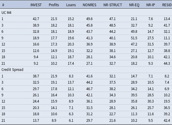
Another way to assess the significance of a particular shock in influencing aggregate private investment growth rate (INVEST) is by computing the fraction of variance it explains in key indicators. To this end, we calculate the forecast error variance decompositions for shocks related to both real user cost M4 growth (UC M4) and credit spread growth (credit spread), with the results presented in Table 2. The corresponding one-step ahead forecasting results are presented in Figures 20 (main model) and 21 (alternative model) in appendices.

Table 2.

Forecast error variance decompositions

Each entry in Table 2 represents the proportion of unexpected volatility in each variable over a 21-month horizon attributed to real user cost M4 and credit spread shocks. The table indicates that, in the very short run (up to nine months), fluctuations in the real user cost M4 growth shock predominantly explain variations in the aggregate private investment growth rate. However, beyond nine months, credit spread shocks become the more influential factor. These findings align with the IRFs depicted in Figure 3.

Nevertheless, fluctuations in the real user cost M4 growth shock primarily account for variations in total corporate profits after tax (Profits), total corporate loans (Loans), non-residential private investment growth rate (NONRES), non-residential structure private investment growth rate (NR-STRUCT), non-residential equipment private investment (NR-EQ), non-residential intellectual property private investment (NR-IP), and residential private investment (RESID) throughout the entire forecast period. These findings further reinforce our earlier conclusion that the real user cost M4 growth shock has a stronger explanatory power than credit spread growth.

3.3. Robustness checks

For robustness checks, we employ alternative measures of the real user cost of money. Our baseline model utilizes the real user cost of M4, excluding Treasury bills. In this section, we consider three additional measures: the real user cost of M4 with Treasury bills (M4T), the real user cost of M3, and the real user cost of all monetary aggregates (All).

Figure 15 presents the IRFs for a shock to the real user cost of M4T. The results indicate that a one percent increase in the standard deviation of the real user cost M4T decreases the aggregate fixed private investment growth rate for seven months without delay, aligning with our main findings. The impact on aggregate corporate profits after tax, total business loans growth, and non-residential and residential private investment growth (including total, structure, equipment, and intellectual property) remains negative, with persistence and magnitude identical to those in our main model.

Similarly, Figure 16 displays the IRFs for a shock to the real user cost of M3. The results show that the impact on all macroeconomic variables (aggregate fixed private investment growth, non-residential fixed private investment growth, and residential fixed private investment growth) and financial variables (aggregate corporate profits after tax and total business loans growth) is consistently negative.

In addition to these two alternative measures, Figure 17 illustrates the impact of the real user cost All, which also exhibits a negative effect on both macroeconomic and financial variables, further reinforcing our main results.

Finally, we adjust the ordering of the economic uncertainty variable in the VAR model, following Jurado et al. (Reference Jurado, Ludvigson and Ng2015). Instead of placing it last, we introduce it as the fourth variable in the macroeconomic block. The results in Figure 18 confirm the findings of our main model, demonstrating that a one percent increase in the standard deviation of the real user cost M4 growth shock leads to declines in aggregate fixed private investment growth, aggregate corporate profits after tax, total business loans growth, and non-residential and residential private investment growth.

Based on these findings, we conclude that our results are robust across different measures of the real user cost of money and adjustments in the VAR model specification.