1 Introduction
Natural thermal convection is fuelled by the variation of the fluid density, that is caused by temperature and pressure variations. The most established model for natural convection flows is the Oberbeck–Boussinesq (OB) approximation (Oberbeck Reference Oberbeck1879; Boussinesq Reference Boussinesq1903). This approximation assumes constant properties, except for the density in the gravitational term which varies linearly with temperature and produces the buoyancy effect. This substantial simplification provided the basis for important advancements in the field, such as the emergence of theories and scaling laws of significant engineering value (e.g. Grossmann & Lohse (Reference Grossmann and Lohse2000)). The limits of applicability of the OB approximation for Rayleigh–Bénard convection, i.e. a fluid layer that is heated from the bottom and cooled from the top, were quantified by Gray & Giorgini (Reference Gray and Giorgini1976). They reported restrictive conditions for the temperature difference, height and Rayleigh number. These conditions are considerably limiting; for example the temperature difference for the case of water must be less than 1.25 K so that the OB approximation is applicable. Despite its notable impact, the range of validity of the OB approximation is too narrow for most thermally driven flows of practical interest.
Inevitably, temperature and pressure variations also affect all other fluid properties in a specific way for each fluid. Therefore, natural thermal convection is manifested in a unique way in different fluids since the effects of property variations are not ‘universal’. The consideration of the property variations gives rise to non-Oberbeck–Boussinesq (NOB) effects, which constitute a deviation from the OB convection (Ahlers Reference Ahlers1980). Common NOB effects in heated cavities are the increase or decrease of the centre temperature and the overall breaking of the symmetry that characterises the OB convection. A number of studies were devoted in the investigation of NOB effects in fluids such as helium (Castaing et al. Reference Castaing, Gunaratne, Heslot, Kadanoff, Libchaber, Thomae, Wu, Zaleski and Zanetti1989), air (Fröhlich, Laure & Peyret Reference Fröhlich, Laure and Peyret1992), corn syrup (Manga & Weeraratne Reference Manga and Weeraratne1999), sulphur hexafluoride (Roy & Steinberg Reference Roy and Steinberg2002), glycol (Xia, Lam & Zhou Reference Xia, Lam and Zhou2002), water (Ahlers et al. Reference Ahlers, Brown, Araujo, Funfschilling, Grossmann and Lohse2006), glycerol (Sugiyama et al. Reference Sugiyama, Calzavarini, Grossmann and Lohse2007) and ethane (Ahlers et al. Reference Ahlers, Calzavarini, Araujo, Funfschilling, Grossmann, Lohse and Sugiyama2008). Several models were also constructed to predict the temperature at the central region of the cavity and other important output parameters for any fluid, given its specific property variations (Wu & Libchaber Reference Wu and Libchaber1991; Ahlers et al. Reference Ahlers, Brown, Araujo, Funfschilling, Grossmann and Lohse2006; Weiss et al. Reference Weiss, He, Ahlers, Bodenschatz and Shishkina2018).
The fluid under investigation in the present study is water. For the range of parameters used here (presented in § 2.3) water properties solely depend on temperature and are insensitive to pressure variations. In their experimental study, Ahlers et al. (Reference Ahlers, Brown, Araujo, Funfschilling, Grossmann and Lohse2006) presented a systematic investigation of the NOB effects on the Rayleigh–Bénard convection inside cylindrical containers filled with water. After identifying the source of the NOB effects on the Nusselt number (
 $Nu$
), the Reynolds number (
 $Re$
) and the centre temperature, they extended the Prandtl–Blasius boundary layer theory for temperature-dependent viscosity and thermal diffusivity. Additional experimental studies were carried out by Brown & Ahlers (Reference Brown and Ahlers2007) who reported temperature measurements outside the boundary layers (BLs) and by Valori et al. (Reference Valori, Elsinga, Rohde, Tummers, Westerweel and van der Hagen2017) who focused on the characterisation of the velocity field in a cubical Rayleigh–Bénard cell.
NOB flows in heated cavities were also studied in terms of direct numerical simulations (DNS). Sugiyama et al. (Reference Sugiyama, Calzavarini, Grossmann and Lohse2009) conducted two-dimensional (2-D) DNS in a closed square Rayleigh–Bénard cell, using temperature-dependent polynomials to model the variation of the water properties. They focused on the flow organisation and investigated the NOB effects on the different velocity scales that can be defined in association with the large-scale circulation (LSC). Moreover, 2-D DNS were also utilised by Kizildag et al. (Reference Kizildag, Rodríguez, Oliva and Lehmkuhl2014) to study the limits of the OB approximation in a water-filled differentially heated cavity, i.e. a closed rectangular cavity heated and cooled by the side walls. They reported that up to a temperature difference of 30 K,
 $Nu$
differs by only approximately
 $1\,\%$
between the OB and the NOB cases. For larger temperature differences, the BLs behave in a qualitatively different way and the inclusion of NOB effects is necessary to accurately capture the flow dynamics. Additionally, Horn & Shishkina (Reference Horn and Shishkina2014) conducted 3-D DNS to study the NOB effects in a cylindrical Rayleigh–Bénard domain, with and without the effects of rotation and Demou, Frantzis & Grigoriadis (Reference Demou, Frantzis and Grigoriadis2018) conducted 2-D and 3-D DNS inside a cuboid cavity.
From a numerical standpoint, thermally driven flows with variable properties constitute a challenging problem. More specifically, the Poisson equation for the pressure that emerges during the numerical solution of the Navier–Stokes equations has variable coefficients, in contrast to OB flows that require the solution of a Poisson equation with constant coefficients. This characteristic drastically increases the computational cost and prohibits the use of efficient fast direct solvers. An indication of this challenge is the very limited number of 3-D DNS studies on this subject. In fact, to the best of the authors’ knowledge, the only 3-D studies on NOB effects available in the literature are those of Horn & Shishkina (Reference Horn and Shishkina2014) and Demou et al. (Reference Demou, Frantzis and Grigoriadis2018) for water, Horn, Shishkina & Wagner (Reference Horn, Shishkina and Wagner2013) for glycerol and Wang et al. (Reference Wang, Xu, Xia, Wan and Sun2017), Liu et al. (Reference Liu, Xia, Yan, Wan and Sun2018) and Demou, Frantzis & Grigoriadis (Reference Demou, Frantzis and Grigoriadis2019) for air. Therefore, the validity of 2-D solutions for the characterisation of the NOB effects becomes an important issue which is relatively unexplored. Within the OB approximation, the differences between 2-D and 3-D simulations were studied by van der Poel, Stevens & Lohse (Reference van der Poel, Stevens and Lohse2013). For Prandtl number
 $Pr=4.38$
(similar to water) and over a wide range of Rayleigh numbers, they reported that although the
 $Nu(Ra)$
scaling is very similar, the temperature profiles and Nusselt numbers are significantly different between 2-D and 3-D solutions. A similar trend was found in the NOB simulations of Demou et al. (Reference Demou, Frantzis and Grigoriadis2018) who reported a deviation in Nusselt number values of 15–20 % between 2-D and 3-D. The difference in other important physical parameters when predicted by 2-D and 3-D NOB simulations is presently unquantified.
Another gap in the NOB literature is the investigation of the modification of the temperature statistics in the near-wall region due to strong property variations. This subject is of significant interest for two main reasons. First of all, almost all of the temperature drop and property variations take place within this narrow near-wall region. Secondly, most of the existing thermal convection theories rely on assumptions for the BL region, such as the extended Prandtl–Blasius boundary layer theory of Ahlers et al. (Reference Ahlers, Brown, Araujo, Funfschilling, Grossmann and Lohse2006). When the predictions of this theory were compared against the detailed DNS results of Sugiyama et al. (Reference Sugiyama, Calzavarini, Grossmann and Lohse2009), the mean temperature profiles in the thermal BLs were found to disagree as early as
 $Ra=10^{8}$
. This disagreement was attributed to the plume activity and the dynamics of the BLs which are not accounted for in the theory. In general, the near-wall distribution of temperature can be divided into three distinct regions, namely the linear, the transitional and the bulk regions (Castaing et al.
Reference Castaing, Gunaratne, Heslot, Kadanoff, Libchaber, Thomae, Wu, Zaleski and Zanetti1989; Wang & Xia Reference Wang and Xia2003; Zhu et al.
Reference Zhu, Mathai, Stevens, Verzicco and Lohse2018). The linear region corresponds to a viscous sublayer, where heat is transferred mainly by conduction. The bulk region exhibits no temperature gradient and it is dominated by convection. The transitional region extends between the linear and the bulk regions and contains the location of maximum temperature root mean square (r.m.s.) as well as the edge of the thermal BL. Even though the mean and r.m.s. temperature distributions in these regions were extensively studied for OB flows, it is unclear how they are influenced by strong property variations.
The present manuscript is focused on the study of Rayleigh–Bénard convection in a rectangular cavity filled with water, taking into account the variation of properties. NOB effects are quantified by evaluating relevant flow parameters such as the Nusselt number, centre temperature, temperature drop inside the boundary layers and boundary layer thickness. More specifically, the main questions to be addressed are the following: (i) what are the differences in the key parameters when predicted by 2-D and 3-D simulations and (ii) how are near-wall distributions of temperature statistics affected by the property variations. The paper is organised as follows: in § 2 the solution methodology is briefly described along with all the necessary definitions and a justification of the numerical parameters adopted. The presentation of the results begins in § 3, where the flow fields are briefly reviewed to visualise the flow and provide the basis of the understanding of some of the differences between the 2-D and 3-D results. The discussion focuses mainly on the LSC which exhibits a qualitatively different behaviour when the third dimension is considered. This is followed by a characterisation of the NOB effects on important output parameters in two dimensions and three dimensions, in § 4. Furthermore, the NOB effects on the near-wall distributions of temperature statistics are presented and discussed in § 5. Finally, the main findings of this study are summarised in § 6.
2 Numerical methodology, definitions and simulation parameters
2.1 Governing equations and numerical implementation
When the OB approximation is applied, the continuity (2.1), Navier–Stokes (2.2) and energy (2.3) equations take the following non-dimensional form:
 $$\begin{eqnarray}\displaystyle & \displaystyle \frac{\unicode[STIX]{x2202}u_{j}}{\unicode[STIX]{x2202}x_{j}}=0, & \displaystyle\end{eqnarray}$$
 $$\begin{eqnarray}\displaystyle & \displaystyle \frac{\unicode[STIX]{x2202}u_{i}}{\unicode[STIX]{x2202}\unicode[STIX]{x1D70F}}+\frac{\unicode[STIX]{x2202}u_{i}u_{j}}{\unicode[STIX]{x2202}x_{j}}=-\frac{\unicode[STIX]{x2202}P}{\unicode[STIX]{x2202}x_{i}}+\frac{Pr}{\sqrt{Ra}}\frac{\unicode[STIX]{x2202}^{2}u_{i}}{\unicode[STIX]{x2202}x_{j}\unicode[STIX]{x2202}x_{j}}+Pr\unicode[STIX]{x1D6E9}\unicode[STIX]{x1D6FF}_{i3}, & \displaystyle\end{eqnarray}$$
 $$\begin{eqnarray}\displaystyle & \displaystyle \frac{\unicode[STIX]{x2202}\unicode[STIX]{x1D6E9}}{\unicode[STIX]{x2202}\unicode[STIX]{x1D70F}}+\frac{\unicode[STIX]{x2202}u_{j}\unicode[STIX]{x1D6E9}}{\unicode[STIX]{x2202}x_{j}}=\frac{1}{\sqrt{Ra}}\frac{\unicode[STIX]{x2202}^{2}\unicode[STIX]{x1D6E9}}{\unicode[STIX]{x2202}x_{j}x_{j}}, & \displaystyle\end{eqnarray}$$
where
 $i=1,2,3$
;
 $x_{i}$
is the non-dimensional Cartesian position vector, also denoted as
 $(x,y,z)$
;
 $u_{i}$
represents the non-dimensional velocity vector, also denoted as
 $(u,v,w)$
. The gravitational acceleration
 $g$
acts along the
 $z$
-direction. Moreover,
 $\unicode[STIX]{x1D70F}$
is the non-dimensional time,
 $P$
the non-dimensional pressure and
 $\unicode[STIX]{x1D6E9}$
the non-dimensional temperature. The scales used to non-dimensionalise these variables are the height of the cavity
 $L_{0}=L$
as the length scale,
 $V_{0}=\bar{\unicode[STIX]{x1D6FC}}\sqrt{Ra}/L_{0}$
as the velocity scale,
 $\unicode[STIX]{x1D70F}_{0}=L_{0}/V_{0}$
as the time scale and
 $P_{0}=\bar{\unicode[STIX]{x1D70C}}{V_{0}}^{2}$
as the pressure scale. Temperature is made non-dimensional as
 $\unicode[STIX]{x1D6E9}=(T-T_{0})/\unicode[STIX]{x0394}T$
, where
 $\unicode[STIX]{x0394}T=T_{b}-T_{t}$
is the temperature difference between the heated (
 $T_{b}$
) and cooled (
 $T_{t}$
) boundaries of the domain. The reference temperature is denoted by
 $T_{0}=(T_{b}+T_{t})/2$
. Using these scales, the characteristic dimensionless groups emerging are the Rayleigh number
 $Ra=g\bar{\unicode[STIX]{x1D6FD}}{L_{0}}^{3}\unicode[STIX]{x0394}T/(\bar{\unicode[STIX]{x1D708}}\bar{\unicode[STIX]{x1D6FC}})$
and the Prandtl number
 $Pr=\bar{\unicode[STIX]{x1D708}}/\bar{\unicode[STIX]{x1D6FC}}$
. The dimensional form of the fluid density, thermal expansion coefficient, kinematic viscosity and thermal diffusivity are denoted as
 $\bar{\unicode[STIX]{x1D70C}}$
,
 $\bar{\unicode[STIX]{x1D6FD}}$
,
 $\bar{\unicode[STIX]{x1D708}}$
and
 $\bar{\unicode[STIX]{x1D6FC}}$
respectively.
Outside the limits of applicability of the OB approximation and in the presence of temperature-dependent properties, the governing equations become,
 $$\begin{eqnarray}\displaystyle & \displaystyle \frac{\unicode[STIX]{x2202}u_{j}}{\unicode[STIX]{x2202}x_{j}}=0, & \displaystyle\end{eqnarray}$$
 $$\begin{eqnarray}\displaystyle & \displaystyle \frac{\unicode[STIX]{x2202}u_{i}}{\unicode[STIX]{x2202}\unicode[STIX]{x1D70F}}+\frac{\unicode[STIX]{x2202}u_{i}u_{j}}{\unicode[STIX]{x2202}x_{j}}=-\frac{1}{\unicode[STIX]{x1D70C}}\frac{\unicode[STIX]{x2202}P}{\unicode[STIX]{x2202}x_{i}}+\frac{1}{\unicode[STIX]{x1D70C}}\frac{Pr}{\sqrt{Ra}}\frac{\unicode[STIX]{x2202}}{\unicode[STIX]{x2202}x_{j}}\left[\unicode[STIX]{x1D707}\left(\frac{\unicode[STIX]{x2202}u_{i}}{\unicode[STIX]{x2202}x_{j}}+\frac{\unicode[STIX]{x2202}u_{j}}{\unicode[STIX]{x2202}x_{i}}\right)\right]+\frac{1}{Fr^{2}}\unicode[STIX]{x1D6FF}_{i3}, & \displaystyle\end{eqnarray}$$
 $$\begin{eqnarray}\displaystyle & \displaystyle \frac{\unicode[STIX]{x2202}\unicode[STIX]{x1D6E9}}{\unicode[STIX]{x2202}\unicode[STIX]{x1D70F}}+\frac{\unicode[STIX]{x2202}u_{j}\unicode[STIX]{x1D6E9}}{\unicode[STIX]{x2202}x_{j}}=\frac{1}{\unicode[STIX]{x1D70C}c_{p}}\frac{1}{\sqrt{Ra}}\frac{\unicode[STIX]{x2202}}{\unicode[STIX]{x2202}x_{j}}\left(k\frac{\unicode[STIX]{x2202}\unicode[STIX]{x1D6E9}}{\unicode[STIX]{x2202}x_{j}}\right), & \displaystyle\end{eqnarray}$$
where the new non-dimensional group emerging is the Froude number
 $Fr=V_{0}/\sqrt{gL_{0}}$
. The non-dimensional forms of density, dynamic viscosity, thermal conductivity and specific heat of the fluid are denoted as
 $\unicode[STIX]{x1D70C},\unicode[STIX]{x1D707},k,$
and
 $c_{p}$
. Since the medium under investigation is water, its fluid properties are effectively independent of pressure and can be approximated by temperature-dependent polynomials. The polynomial expressions that were used in the present study are listed in table 1. These fluid properties were non-dimensionalised using the value of each property at the reference temperature, e.g.
 $k(T)=\bar{k}(T)/\bar{k}(T_{0})$
.
Coefficients
 $a_{n}$
of the polynomials
 $(X-X_{0})/X_{0}=\sum _{n=1}^{3}a_{n}(T-T_{0})^{n}$
describing the temperature dependence of a property
 $X$
of water. The reference temperature is
 $T_{0}=313~\text{K}$
and the polynomials are accurate over the range
 $283<T<343~\text{K}$
(Ahlers et al.
Reference Ahlers, Brown, Araujo, Funfschilling, Grossmann and Lohse2006).

Both the OB set of equations (2.1)–(2.3) and the NOB set of equations (2.4)–(2.6) were used in this study. The numerical solution followed the fractional-step method, using second-order central differences for space discretisation and a fully explicit, second-order Adams–Bashforth scheme to advance the solution in time. Specifically for the NOB cases, a pressure-splitting technique was utilised for the transformation of the derived variable coefficients Poisson equation for the pressure into a constant coefficients equation. The Poisson equation for both cases was solved by performing a parallel forward and inverse fast Fourier transform along a homogeneous direction. A comprehensive presentation of the numerical methodology along with details about the numerical implementation and its validation can be found in the study of Demou et al. (Reference Demou, Frantzis and Grigoriadis2018).
2.2 Definitions
This section presents the definitions of the main parameters that are evaluated for the characterisation of the NOB effects. The bracket notation
 $\langle \unicode[STIX]{x1D719}\rangle _{a,b,...}$
denotes the averaging of a variable
 $\unicode[STIX]{x1D719}$
with respect to variables
 $a,b$
, etc. Therefore, the mean and r.m.s. values of a variable
 $\unicode[STIX]{x1D719}$
are denoted as
 $\langle \unicode[STIX]{x1D719}\rangle _{\unicode[STIX]{x1D70F}}$
and
 $\unicode[STIX]{x1D719}_{rms}$
where
 $\unicode[STIX]{x1D719}_{rms}=(\langle \unicode[STIX]{x1D719}^{2}\rangle _{\unicode[STIX]{x1D70F}}-\langle \unicode[STIX]{x1D719}\rangle _{\unicode[STIX]{x1D70F}}^{2})^{1/2}$
. Following this notation, the time-varying, area-averaged Nusselt numbers along the bottom
 $Nu_{b}(\unicode[STIX]{x1D70F})$
and top
 $Nu_{t}(\unicode[STIX]{x1D70F})$
walls are defined as,
 $$\begin{eqnarray}\displaystyle Nu_{b}(\unicode[STIX]{x1D70F})=-k_{b}\left.\frac{\unicode[STIX]{x2202}\langle \unicode[STIX]{x1D6E9}\rangle _{x,y}}{\unicode[STIX]{x2202}z}\right|_{z=0},\quad Nu_{t}(\unicode[STIX]{x1D70F})=-k_{t}\left.\frac{\unicode[STIX]{x2202}\langle \unicode[STIX]{x1D6E9}\rangle _{x,y}}{\unicode[STIX]{x2202}z}\right|_{z=1}, & & \displaystyle\end{eqnarray}$$
where it is assumed that the bottom wall is located at
 $z=0$
and the top wall at
 $z=1$
. The time- and area-averaged Nusselt numbers are simply denoted as
 $Nu_{b}=\langle Nu_{b}(\unicode[STIX]{x1D70F})\rangle _{\unicode[STIX]{x1D70F}}$
for the bottom wall and
 $Nu_{t}=\langle Nu_{t}(\unicode[STIX]{x1D70F})\rangle _{\unicode[STIX]{x1D70F}}$
for the top wall. Moreover, the centre temperature of the cavity
 $\unicode[STIX]{x1D6E9}_{c}$
is defined as,
 $$\begin{eqnarray}\displaystyle \unicode[STIX]{x1D6E9}_{c}=\langle \unicode[STIX]{x1D6E9}\rangle _{\unicode[STIX]{x1D70F},x,y}|_{z=0.5}. & & \displaystyle\end{eqnarray}$$
In OB flows the mean temperature field is symmetric around the centre of the cavity, therefore
 $\unicode[STIX]{x1D6E9}_{c}=0$
. Because of the property variations, in NOB flows this symmetry is lost and
 $\unicode[STIX]{x1D6E9}_{c}\neq 0$
. One can also define an additional associated parameter which quantifies the temperature drop across the bottom and top BLs, denoted as
 $\unicode[STIX]{x1D6E5}_{b}$
and
 $\unicode[STIX]{x1D6E5}_{t}$
respectively. Since there is no significant temperature drop across the bulk of the cavity, these temperature drops can be approximated as,
 $$\begin{eqnarray}\displaystyle \unicode[STIX]{x1D6E5}_{b}=\langle \unicode[STIX]{x1D6E9}\rangle _{\unicode[STIX]{x1D70F},x,y}|_{z=0}-\unicode[STIX]{x1D6E9}_{c},\quad \unicode[STIX]{x1D6E5}_{t}=\unicode[STIX]{x1D6E9}_{c}-\langle \unicode[STIX]{x1D6E9}\rangle _{\unicode[STIX]{x1D70F},x,y}|_{z=1}, & & \displaystyle\end{eqnarray}$$
where in this study,
 $\langle \unicode[STIX]{x1D6E9}\rangle _{\unicode[STIX]{x1D70F},x,y}|_{z=0}$
and
 $\langle \unicode[STIX]{x1D6E9}\rangle _{\unicode[STIX]{x1D70F},x,y}|_{z=1}$
coincide with the imposed boundary conditions along the bottom and the top walls respectively. From these definitions, one can easily obtain the relation
 $\unicode[STIX]{x1D6E5}_{b}+\unicode[STIX]{x1D6E5}_{t}=1.0$
. Finally, the thermal BL thickness
 $\unicode[STIX]{x1D706}^{\unicode[STIX]{x1D703}}$
is evaluated using the temperature slope along each horizontal wall, i.e.
 $$\begin{eqnarray}\displaystyle \unicode[STIX]{x1D706}_{b}^{\unicode[STIX]{x1D703}}=\frac{\unicode[STIX]{x1D6E5}_{b}}{\left.-\displaystyle \frac{\unicode[STIX]{x2202}\langle \unicode[STIX]{x1D6E9}\rangle _{\unicode[STIX]{x1D70F},x,y}}{\unicode[STIX]{x2202}z}\right|_{z=0}},\quad \unicode[STIX]{x1D706}_{t}^{\unicode[STIX]{x1D703}}=\frac{\unicode[STIX]{x1D6E5}_{t}}{\left.-\displaystyle \frac{\unicode[STIX]{x2202}\langle \unicode[STIX]{x1D6E9}\rangle _{\unicode[STIX]{x1D70F},x,y}}{\unicode[STIX]{x2202}z}\right|_{z=1}}. & & \displaystyle\end{eqnarray}$$
2.3 Simulation parameters
To address the underlying questions posed in the present study, a series of 2-D and 3-D DNS were conducted for Rayleigh–Bénard convection in a cavity filled with water, as shown in figure 1. The physical and numerical parameters used for all simulated cases are listed in table 2 and the justification for the selection of each parameter is discussed below. The Rayleigh number varied in the range of
 $10^{6}\leqslant Ra\leqslant 10^{9}$
. The temperature difference
 $\unicode[STIX]{x0394}T$
between the two horizontal walls varied up to
 $60~\text{K}$
, around a reference temperature of
 $T_{0}=313~\text{K}$
, where
 $Pr=4.38$
. Since
 $\unicode[STIX]{x0394}T$
is a control parameter in the simulations, it is assumed that the variation of
 $Ra$
is achieved with a corresponding increase/decrease of the cavity dimensions, without altering its aspect ratio. For cases with
 $\unicode[STIX]{x0394}T\approx 0$
, the OB approximation was applied (equations (2.1)–(2.3)). For all other cases, the NOB set of equations were used (equations (2.4)–(2.6)) and the fluid properties were allowed to vary according to the temperature polynomials presented in table 1.
Physical and numerical parameters used for each simulation. Cases with
 $\unicode[STIX]{x0394}T\approx 0$
were computed using the OB approximation.
 $h$
denotes the local grid spacing and
 $h_{BL}$
the maximum grid spacing inside the thermal BLs.
 $h_{BL}^{th}$
denotes a theoretical estimate for the maximum grid spacing inside the thermal BLs as suggested by Shishkina et al. (Reference Shishkina, Stevens, Grossmann and Lohse2010).
 $\unicode[STIX]{x1D702}_{B}$
denotes the Batchelor length scale.
 $\unicode[STIX]{x0394}\unicode[STIX]{x1D70F}_{s}$
represents the time interval used for statistical sampling.

Cuboid cavity used for the 3-D simulations, with
 $L_{x}=L_{z}$
.

Both the 2-D and 3-D geometries are confined by solid walls in the
 $x$
- and
 $z$
-direction, while a periodic spanwise
 $y$
-direction is present only in the 3-D cases. The absence of side walls along the
 $y$
-direction for the 3-D cases provides an appropriate basis for the comparison between the 2-D and 3-D solutions because the 3-D character of the flow is not induced or affected by the presence of side walls along the
 $y$
-direction. The cavity has a square cross-section (
 $L_{x}=L_{z}=1$
) while the size of the computational box along the periodic direction
 $L_{y}$
was chosen so that the structures of the flow were not suppressed due to the imposed periodicity. Similar to the studies of Trias et al. (Reference Trias, Soria, Oliva and Pérez-Segarra2007) and Sebilleau et al. (Reference Sebilleau, Issa, Lardeau and Walker2018), the selection of a sufficient length for
 $L_{y}$
was guided by the calculation of the spanwise two-point correlations of the wall-normal velocity components,
 $$\begin{eqnarray}\displaystyle R_{uu}(x,y,z)=\frac{\langle u^{\prime }(x,0,z)u^{\prime }(x,y,z)\rangle _{\unicode[STIX]{x1D70F}}}{\langle u^{\prime 2}\rangle _{\unicode[STIX]{x1D70F}}},\quad R_{ww}(x,y,z)=\frac{\langle w^{\prime }(x,0,z)w^{\prime }(x,y,z)\rangle _{\unicode[STIX]{x1D70F}}}{\langle w^{\prime 2}\rangle _{\unicode[STIX]{x1D70F}}}, & & \displaystyle \nonumber\\ \displaystyle & & \displaystyle\end{eqnarray}$$
where
 $u^{\prime }$
and
 $w^{\prime }$
are the wall-normal fluctuating velocity components, defined as
 $u^{\prime }=u-\langle u\rangle _{\unicode[STIX]{x1D70F}}$
and
 $w^{\prime }=w-\langle w\rangle _{\unicode[STIX]{x1D70F}}$
respectively. The spanwise length of the domain can be considered as adequate when these fluctuating components become uncorrelated and two-point correlations are significantly reduced. In general, since the turbulent structures in the flow become finer as
 $Ra$
increases, simulations at lower
 $Ra$
are more demanding in terms of length for the periodic direction. Figure 2 presents the two-point correlations for the two wall-normal velocity components at the locations of the maximum temperature r.m.s. in the vicinity of the top and bottom walls, for the lowest Rayleigh number considered,
 $Ra=10^{6}$
. For both velocity components, the two-point correlations reduce significantly within a distance smaller than
 $L_{y}/2$
and uncorrelated turbulent fluctuations are obtained within this length. Therefore, a spanwise extend of
 $L_{y}=\unicode[STIX]{x03C0}$
can be justified as adequate for cases at
 $Ra=10^{6}$
. This was also verified by performing an additional simulation with a twice-as-long spanwise extent (not shown here), which revealed that the values of the Nusselt number and volume-averaged temperature changed by less than
 $0.08\,\%$
. A similar two-point correlation analysis for cases at higher
 $Ra$
revealed that the appropriate length could not be substantially reduced. Therefore, the same periodic length
 $L_{y}=\unicode[STIX]{x03C0}$
was used for all 3-D cases up to
 $Ra=10^{9}$
.
Two-point correlations of the wall-normal velocity components
 $R_{uu}$
and
 $R_{ww}$
for case
 $A40$
. The calculations were carried out at the locations of the maximum temperature r.m.s., in the vicinity of the top and bottom walls: dashed line,
 $(x,z)=(0.5,0.934)$
; solid line,
 $(x,z)=(0.5,0.053)$
.

A structured Cartesian grid was used in all cases. More specifically, the grid was equidistant along the periodic
 $y$
-direction and stretched in the
 $x$
–
 $z$
planes following a linear expansion to allow the clustering of computational grid points next to the solid walls. The resolution along the
 $y$
-direction and in each
 $x$
–
 $z$
plane was determined after a set of preliminary simulations, where successively finer grids were used up to the point where the calculated output parameters were almost independent of the grid resolution. Also, the quality of the adopted grid was tested a posteriori following the criteria suggested by Shishkina et al. (Reference Shishkina, Stevens, Grossmann and Lohse2010) for OB flows. The first criterion sets maximum-bound estimates for the grid spacing
 $h_{BL}^{th}$
inside the thermal BL which, for the case of water, is thinner than the velocity BL. For
 $Pr=4.38$
, the criterion suggests
 $h_{BL}^{th}=2^{-1.5}\unicode[STIX]{x1D6FC}^{-1}E^{-1.5}Nu^{-1.5}$
, where
 $\unicode[STIX]{x1D6FC}=0.482$
and
 $E=0.982$
. As shown in table 2, the maximum grid spacing
 $h_{BL}$
used here to resolve the thermal BLs was less than half of
 $h_{BL}^{th}$
for all the simulations presented. Due to the variation of the water properties in the NOB simulations, the bottom thermal BL is expected to be thinner than the top one, increasing the resolution requirements in the vicinity of the bottom wall. However, since part of this study focuses on the differences between the top and bottom parts of the cavity, the finer grid spacing was used for both the bottom and the top, so that any reported asymmetries are not attributed to the computational grid. The second criterion sets the resolution requirements in the bulk of the cavity where the largest grid spacing should be comparable to the global Batchelor length scale
 $\unicode[STIX]{x1D702}_{B}$
which, for the present set of parameters, is smaller compared to the global Kolmogorov length scale. The global Batchelor length scale is defined as
 $\unicode[STIX]{x1D702}_{B}=\langle (\unicode[STIX]{x1D708}\unicode[STIX]{x1D6FC}^{2}/\unicode[STIX]{x1D716}_{u})^{0.25}\rangle _{\unicode[STIX]{x1D70F},V}$
, where
 $\unicode[STIX]{x1D716}_{u}$
is the local kinetic energy dissipation rate per mass and
 $V$
the volume of the domain. The maximum ratio between the local grid spacings used in the simulations
 $h$
and the global Batchelor length scale is shown in table 2, where
 $h$
is less than or comparable to
 $\unicode[STIX]{x1D702}_{B}$
in the entire domain.
For 2-D simulations, a stagnant flow condition was used as the initial condition. For 3-D simulations, the initial field consisted of a statistically stationary solution of the corresponding 2-D case. Random perturbations with a Gaussian distribution and an intensity of
 $5\,\%$
based on the local velocity magnitude were superimposed to trigger transition to a 3-D turbulent regime. The simulations advanced in time using a dynamically adjusted time step
 $\unicode[STIX]{x0394}\unicode[STIX]{x1D70F}$
which was restricted according to the Courant–Friedrichs–Lewy condition (
 $CFL$
) and the viscous stability limit (
 $VSL$
), namely,
 $$\begin{eqnarray}\displaystyle CFL=\frac{u_{i}\unicode[STIX]{x0394}\unicode[STIX]{x1D70F}}{h_{i}}<CFL_{max}\quad \text{and}\quad VSL=\frac{\unicode[STIX]{x1D708}\unicode[STIX]{x0394}\unicode[STIX]{x1D70F}}{u_{i}^{2}}<VSL_{max}, & & \displaystyle\end{eqnarray}$$
where
 $u_{i}$
and
 $h_{i}$
are the local velocity and grid spacing along the
 $i\text{th}$
direction and
 $(CFL_{max},VSL_{max})=(0.2,0.05)$
.
Each simulation was allowed to develop for an initial period so that a statistically stationary state was reached before commencing statistical sampling. The determination of the appropriate development period was guided by examining the time evolution of the instantaneous Nusselt number. A typical time evolution of
 $Nu_{b}(\unicode[STIX]{x1D70F})$
is shown in figure 3(a) for case D40-2D. Statistical stationarity was identified at time
 $\unicode[STIX]{x1D70F}=\unicode[STIX]{x1D70F}_{s}$
using the ratio of the temporally averaged Nusselt numbers at the top and bottom walls,
 $$\begin{eqnarray}\displaystyle \frac{\langle Nu_{t}(\unicode[STIX]{x1D70F})\rangle _{\unicode[STIX]{x1D70F}}}{\langle Nu_{b}(\unicode[STIX]{x1D70F})\rangle _{\unicode[STIX]{x1D70F}}}=\frac{\displaystyle \int _{0}^{\unicode[STIX]{x1D70F}}Nu_{t}(\hat{\unicode[STIX]{x1D70F}})\,\text{d}\hat{\unicode[STIX]{x1D70F}}}{\displaystyle \int _{0}^{\unicode[STIX]{x1D70F}}Nu_{b}(\hat{\unicode[STIX]{x1D70F}})\,\text{d}\hat{\unicode[STIX]{x1D70F}}}. & & \displaystyle\end{eqnarray}$$
Under a statistically stationary condition, the heat transferred in the cavity from the heated wall is balanced by the heat leaving the system from the cooled wall, therefore the ratio defined in equation (2.13) approaches unity for both the OB and NOB cases. Figure 3(b) shows that for case D40-2D, statistical stationarity was identified at
 $\unicode[STIX]{x1D70F}_{s}\approx 300$
. Once statistical stationarity was reached, an appropriate sampling period
 $\unicode[STIX]{x0394}\unicode[STIX]{x1D70F}_{s}$
was defined for each case (last column of table 2). This was determined by increasing the statistical sample so that the statistics were independent of the sample size. In practice, statistics were collected until the maximum r.m.s. values of the temperature field deviated by less than
 $2\,\%$
compared to values obtained with
 $\unicode[STIX]{x0394}\unicode[STIX]{x1D70F}_{s}/2$
. An a posteriori verification of this procedure can be obtained by calculating the ratio,
 $$\begin{eqnarray}\displaystyle \frac{\langle Nu_{b,t}(\unicode[STIX]{x1D70F})\rangle _{\unicode[STIX]{x1D70F}}}{\langle Nu_{b,t}(\unicode[STIX]{x1D70F})\rangle _{\unicode[STIX]{x0394}\unicode[STIX]{x1D70F}_{s}}}=\frac{\displaystyle \int _{\unicode[STIX]{x1D70F}_{s}}^{\unicode[STIX]{x1D70F}_{s}+\unicode[STIX]{x1D70F}}Nu_{b,t}(\hat{\unicode[STIX]{x1D70F}})\,\text{d}\hat{\unicode[STIX]{x1D70F}}}{\displaystyle \int _{\unicode[STIX]{x1D70F}_{s}}^{\unicode[STIX]{x1D70F}_{s}+\unicode[STIX]{x0394}\unicode[STIX]{x1D70F}_{s}}Nu_{b,t}(\hat{\unicode[STIX]{x1D70F}})\,\text{d}\hat{\unicode[STIX]{x1D70F}}}. & & \displaystyle\end{eqnarray}$$
This ratio is plotted for the bottom wall in the inset of figure 3(b) for case D40-2D, where
 $\unicode[STIX]{x0394}\unicode[STIX]{x1D70F}_{s}=400$
. The statistical errors on the Nusselt number (
 $\unicode[STIX]{x1D6FF}Nu$
) were calculated using the relation
 $\unicode[STIX]{x1D6FF}Nu=Nu_{rms}(2\unicode[STIX]{x1D70F}_{I}/\unicode[STIX]{x0394}\unicode[STIX]{x1D70F}_{s})^{1/2}$
, where
 $\unicode[STIX]{x1D70F}_{I}$
is the integral time obtained from the autocorrelation coefficient of
 $Nu$
. The largest statistical error on the Nusselt number was calculated 0.33 % for case D60-2D. The statistical error on the other reported output parameters is much smaller due to low r.m.s. values.
Case D40-2D. (a) Temporal variation of the Nusselt number at the bottom wall and (b) ratios of temporally averaged Nusselt number, described by (2.13) and (2.14) (inset). For this case, the flow reaches a statistically steady state at
 $\unicode[STIX]{x1D70F}_{s}\approx 300$
, and a sample period of
 $\unicode[STIX]{x0394}\unicode[STIX]{x1D70F}_{s}\approx 400$
is sufficient for statistical sampling.

3 Flow organisation
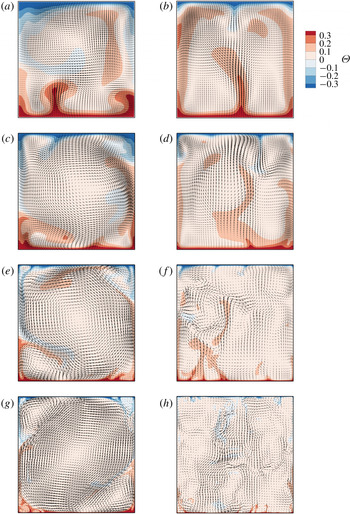
Even though the instantaneous fields cannot be used to quantify the NOB effects, they are helpful in obtaining a first appreciation of the main differences between the 2-D and 3-D solutions. Figure 4 illustrates instantaneous temperature contours along with velocity vectors at the
 $x$
–
 $z$
plane for the 2-D and 3-D simulations with
 $\unicode[STIX]{x0394}T=40~\text{K}$
. In both the 2-D and 3-D cases, hot and cold plumes were found to eject from the bottom and top boundary layers respectively. As expected, the structure of these plumes became finer as
 $Ra$
increased and by
 $Ra=10^{9}$
most of the cavity was nearly isothermal.
Instantaneous temperature contours with velocity vectors at the
 $x$
–
 $z$
plane for 2-D (a,c,e,g) and 3-D (b,d,f,h) simulations with
 $\unicode[STIX]{x0394}T=40~\text{K}$
, at
 $Ra=10^{6}$
(a,b),
 $Ra=10^{7}$
(c,d),
 $Ra=10^{8}$
(e,f) and
 $Ra=10^{9}$
(g,h). These instantaneous fields are snapshots of the flow after statistical stationarity was reached. For the 3-D cases, the snapshots were taken at
 $y=0$
. The range
 $[-0.3,0.3]$
is used in the colour bars instead of the full normalised temperature range
 $[-0.5,0.5]$
so that the structures of the flow are better illustrated. For clarity, the velocity vectors are only shown every second, sixth and twelfth grid node in each direction for (c,d), (e,f) and (g,h) respectively.

In the 2-D cases, the plumes fed the LSC that covered the central area of the cavity for the whole
 $Ra$
range. The LSC was accompanied by two counter-rotating vortices that were located at two opposite corners of the cavity. The vortex in the vicinity of the heated wall exhibited stronger rotation due to lower viscosity, compared to the vortex at the vicinity of the cooled wall, something that was first reported by Sugiyama et al. (Reference Sugiyama, Calzavarini, Grossmann and Lohse2009). Interestingly, as shown in figure 4, there were no indications of a LSC in the
 $x$
–
 $z$
planes of the 3-D solutions. The absence of the LSC in the
 $x$
–
 $z$
planes modified the locations where plumes were ejected from the top and the bottom BLs. More specifically, in 3-D cases, plumes were captured to eject from any
 $x$
-location, while the presence of an LSC in the 2-D solutions favoured the ejection of plumes closer to the side walls. Counter to what was observed in the
 $x$
–
 $z$
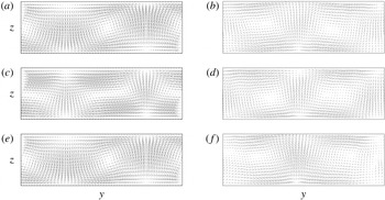
planes of the 3-D solutions, the visualisation of the flow in the
 $y$
–
 $z$
planes provides clear evidence of LSC structures. The time-averaged velocity vectors in three different
 $y$
–
 $z$
planes for cases A40 and D40 are shown in figure 5. In both cases, a strong 3-D character is revealed with significant variations along the spanwise direction. More specifically, the flow appears to be well organised with two similar but clearly distinguishable LSC structures along the
 $y$
–
 $z$
planes. The location of the interaction of two LSC structures was typically accompanied by long plumes ejected from the BLs.
Time-averaged velocity vectors in the
 $y$
–
 $z$
planes located at (a,b)
 $x=0.1$
, (c,d)
 $x=0.5$
and (e,f)
 $x=0.9$
, for the 3-D cases with
 $\unicode[STIX]{x0394}T=40~\text{K}$
, at
 $Ra=10^{6}$
(a,c,e),
 $Ra=10^{9}$
(b,d,f). For clarity, the presented results were interpolated on a coarser grid of
 $N_{y}\times N_{z}=60\times 20$
.

With respect to the dynamic features of the flow, the LSC in the 2-D cases exhibited random reversals, caused by the increase in size of the corner vortices to the point where the LSC ceases and restarts in a reversed rotation state. For
 $Ra=10^{6}$
the reversals were so frequent that the system spent more time in the cessation and reversal process than in a LSC mode, which appeared only sparingly. As
 $Ra$
increased, the LSC was found to be more stable and the cessation-reversal process happened more and more rarely. This is in line with the OB study of Sugiyama et al. (Reference Sugiyama, Ni, Stevens, Chan, Zhou, Xi, Sun, Grossmann, Xia and Lohse2010) who used a fluid with a similar Prandtl number and concluded that, for 2-D systems at
 $Ra=10^{9}$
, the mean time interval between two successive reversals increases by three orders of magnitude compared to
 $Ra=10^{8}$
. For NOB conditions, Sugiyama et al. (Reference Sugiyama, Calzavarini, Grossmann and Lohse2009) studied in detail the LSC characteristics in a 2-D square cavity adopting a conditional time-averaging procedure. More specifically, the sign of the vorticity at the centre of the cavity was used to identify the reversals of the LSC structure. At the event of a reversal, the velocity field was mirrored along the vertical centreline and the time-averaging procedure continued. This approach helps in the visualisation of the time-averaged LSC structure which otherwise would vanish due to nearly zero time-averaged velocities everywhere. Unlike the 2-D cases, the LSC structures in the 3-D solutions did not exhibit any reversals, despite the large sampling periods considered here. Consequently the visualisation of the 3-D LSC structures does not require a conditional time-averaging approach.
Considering these flow features, instead of adopting a conditional time-averaging procedure in the present study, the findings of Sugiyama et al. (Reference Sugiyama, Calzavarini, Grossmann and Lohse2009) for the 2-D square cavity are used to compare the most important LSC characteristics in the 3-D cuboid cavity considered here. The following differences were revealed:
(i) Size and shape: the 2-D LSC structures were found to be suppressed due to the presence of the small counter-rotating vortices, adopting a slightly elongated shape along one of the cavity’s diagonal. On the other hand, the LSC structures in three dimensions appeared elongated along the
 $y$
-direction, with an aspect ratio of
$\unicode[STIX]{x03C0}/2$
in all cases. The 3-D structures extend along the
$x$
-direction and the LSC breaks down only very close to the vertical side walls.
(ii) Velocity distributions: Sugiyama et al. (Reference Sugiyama, Calzavarini, Grossmann and Lohse2009) reported vertical distributions of the horizontally averaged and conditional time-averaged
$x$
-velocity component
$\langle u\rangle _{t,x}$
for a 2-D cavity. Since the LSC in the 3-D geometry considered here was found aligned with the
$y$
–
$z$
plane, the 3-D equivalent should be the horizontally and time-averaged
$y$
-velocity component
$\langle v\rangle _{t,x,y}$
within one LSC structure. Figure 6 shows these distributions for
$Ra=10^{6}{-}10^{9}$
and
$\unicode[STIX]{x0394}T=40~\text{K}$
, including the results by Sugiyama et al. (Reference Sugiyama, Calzavarini, Grossmann and Lohse2009) which are available for
$Ra=10^{6}$
and
$10^{8}$
. It is revealed that the maxima of the 3-D distributions are located closer to the top and bottom walls, compared to the 2-D distributions. Consequently, the near-wall regions at the top and at the bottom of the cavity experience significantly larger velocities in three dimensions than two dimensions.


Time- and space-averaged velocity distributions for
 $\unicode[STIX]{x0394}T=40~\text{K}$
and (a)
 $Ra=10^{6}$
, (b)
 $Ra=10^{7}$
, (c)
 $Ra=10^{8}$
and (d)
 $Ra=10^{9}$
. Solid lines: present 3-D results of
 $\langle v\rangle _{t,x,y}$
within one LSC structure. Since there are two counter-rotating LSC structures along the spanwise direction, one of these structures was mirrored across the
 $z$
-axis and a mean distribution for both LSCs is presented. Dashed lines: 2-D results of
 $\langle u\rangle _{t,x,y}$
presented by Sugiyama et al. (Reference Sugiyama, Calzavarini, Grossmann and Lohse2009) who followed a conditional time-averaging procedure to address the random reversals of the LSC structure in two dimensions.

This brief investigation of the flow organisation revealed significant qualitative and quantitative differences between the 2-D and the 3-D flow fields. The effects of these differences on the NOB characteristics of the flow are quantified by the statistical analysis presented in the following sections. The presence of LSC structures in a different plane (
 $y$
–
 $z$
in three dimensions and
 $x$
–
 $z$
in two dimensions) and the chaotic nature of the LSC reversals in the 2-D cases complicates the comparison of the time-averaged velocity fields between the 2-D and 3-D cases. For these reasons, the present work only focuses on the statistics of the temperature field and other derived quantities. To perform a fair comparison between the 2-D and the 3-D cases,
 $x$
–
 $y$
-plane-averaged temperature statistics from 3-D cases are compared against the corresponding
 $x$
-line-averaged statistics from 2-D cases.
(a) Reduced Nusselt number values, scaled with
 $Ra^{1/3}$
and (b) Nusselt number values normalised with the respective OB values, as a function of
 $Ra$
for
 $\unicode[STIX]{x0394}T=40~\text{K}$
: open squares, present 2-D results; solid squares, present 3-D results; open circles, 2-D numerical results reported by Sugiyama et al. (Reference Sugiyama, Calzavarini, Grossmann and Lohse2009); diamonds, numerical results in a cylindrical domain reported by Horn & Shishkina (Reference Horn and Shishkina2014).

4 Output parameters
4.1 Nusselt number
Values of the reduced Nusselt number
 $Nu/Ra^{1/3}$
from 2-D and 3-D simulations for
 $\unicode[STIX]{x0394}T=40~\text{K}$
are shown in figure 7(a). Throughout the
 $Ra$
range, the 3-D predictions of
 $Nu$
are higher than the corresponding 2-D predictions. The numerical results of Horn & Shishkina (Reference Horn and Shishkina2014) are also shown in figure 7(a) and, even though this study considered cylindrical geometries, the absolute values and the overall trend are similar to the 3-D simulations of the present study. Nevertheless, the deviation percentage
 $(Nu_{3D}-Nu_{2D})/Nu_{3D}$
exhibits no systematic change, ranging between 15 % and 20 %. This can be rationalised by referencing the space-averaged velocity distributions shown in figure 6. The part of the LSC structure that is located closer to the top and bottom walls exhibits larger horizontal velocities in three dimensions than in two dimensions. This characteristic leads to stronger interaction between the LSC and the boundary layers, and consequently affects the near-wall temperature gradients, shown in table 3. The 3-D cases exhibit sharper temperature gradients on both the bottom and the top walls, resulting in enhanced heat transfer rates compared to the 2-D cases. A similar finding was reported by van der Poel et al. (Reference van der Poel, Stevens and Lohse2013) who carried out a comparison of two dimensions versus three dimensions within the OB approximation and attributed the differences in Nusselt number to the qualitatively different characteristics of the 2-D and 3-D LSC structures.
Moreover, the prefactor
 $a$
and the exponent
 $\unicode[STIX]{x1D6FE}$
in the
 $Nu=aRa^{\unicode[STIX]{x1D6FE}}$
power law were calculated using a least-squares fit on a single power law. These parameters were predicted to be
 $a=0.118$
and
 $\unicode[STIX]{x1D6FE}=0.292$
for the 2-D set of simulations and
 $a=0.145$
and
 $\unicode[STIX]{x1D6FE}=0.291$
for the 3-D set. The values for the scaling exponent
 $\unicode[STIX]{x1D6FE}$
are similar to those obtained by earlier experimental studies of thermal convection in water using lower
 $\unicode[STIX]{x0394}T$
(within the OB approximation) and different geometries. For example, Garon & Goldstein (Reference Garon and Goldstein1973) reported
 $\unicode[STIX]{x1D6FE}=0.293$
using a cylindrical cell and Hiroaki & Hiroshi (Reference Hiroaki and Hiroshi1980) reported
 $\unicode[STIX]{x1D6FE}=0.290$
using a cuboid cell.
Time- and space-averaged temperature gradients along the top (
 $\unicode[STIX]{x2202}\langle \unicode[STIX]{x1D6E9}\rangle _{x,y}/\unicode[STIX]{x2202}z|_{z=1}$
) and bottom (
 $(\unicode[STIX]{x2202}\langle \unicode[STIX]{x1D6E9}\rangle _{x,y}/\unicode[STIX]{x2202}z)|_{z=0}$
) walls, for
 $\unicode[STIX]{x0394}T=40~\text{K}$
.

To identify how the NOB effects modify the Nusselt number, the calculated
 $Nu$
values from NOB simulations with
 $\unicode[STIX]{x0394}T=40~\text{K}$
are normalised with the respective OB values and presented in figure 7(b) as a function of
 $Ra$
. Focusing first on the 3-D results, the
 $Nu_{NOB}/Nu_{OB}$
ratio is nearly constant, close to a value of
 $0.98$
throughout the
 $Ra$
range considered. This is not the case for the 2-D results, where this ratio changes abruptly with a clearly noticeable peak at
 $Ra=10^{8}$
. A similar peak was present in the 2-D numerical results of Sugiyama et al. (Reference Sugiyama, Calzavarini, Grossmann and Lohse2009), also shown in figure 7(b), although these results reveal slightly weaker NOB effects compared to the 2-D results of the present study. This is attributed to the fact that Sugiyama et al. (Reference Sugiyama, Calzavarini, Grossmann and Lohse2009) used a different set of equations compared to equations (2.4)–(2.6). More specifically, they considered constant values for
 $\bar{C}_{p}$
and
 $\bar{\unicode[STIX]{x1D70C}}$
everywhere except in the buoyancy term, where
 $\bar{\unicode[STIX]{x1D70C}}$
followed a similar temperature polynomial as the one used here. Since the governing equations used in the present study consider variable properties in all terms, the slightly stronger NOB effects are justified.
A more systematic investigation of the
 $Nu$
variation with
 $\unicode[STIX]{x0394}T$
is shown in figure 8(a) for
 $Ra=10^{9}$
. A weak gradual decrease of
 $Nu$
as
 $\unicode[STIX]{x0394}T$
increases is revealed for both the 2-D and 3-D cases. Even though the decreasing trend looks similar for the two different sets of simulations, the normalised
 $Nu_{NOB}/Nu_{OB}$
results, shown in figure 8(b), reveal a slightly more rapid strengthening of the NOB effects in three dimensions compared to the 2-D results. For comparison purposes, figure 8(b) also shows the 2-D numerical results of Sugiyama et al. (Reference Sugiyama, Calzavarini, Grossmann and Lohse2009) and the 3-D numerical results of Horn & Shishkina (Reference Horn and Shishkina2014). Although differences between the present 2-D and 3-D results and other geometries are visible, overall, the NOB effects on the Nusselt number are very weak, in line with the extended BL theory developed by Ahlers et al. (Reference Ahlers, Brown, Araujo, Funfschilling, Grossmann and Lohse2006).
(a) Nusselt number values and (b) Nusselt number values normalised with the respective OB values as a function of
 $\unicode[STIX]{x0394}T$
for
 $Ra=10^{9}$
: open squares, present 2-D results; solid squares, present 3-D results; open circles, 2-D numerical results reported by Sugiyama et al. (Reference Sugiyama, Calzavarini, Grossmann and Lohse2009) at
 $Ra=10^{8}$
; diamonds, 3-D numerical results in a cylindrical domain reported by Horn & Shishkina (Reference Horn and Shishkina2014).

4.2 Centre temperature
For Rayleigh–Bénard convection within the limits of the OB approximation, the time-averaged temperature field is symmetric around the centre of the cavity. Consequently, the temperature at the centre of the cavity is equal to the mean temperature between the heated and cooled walls. For NOB convection with variable properties, the temperature at the cavity core deviates from the mean wall temperature. To quantify this effect, figure 9 shows the centre temperature
 $\unicode[STIX]{x1D6E9}_{c}$
(defined by equation (2.8)) plotted against
 $\unicode[STIX]{x0394}T$
and
 $Ra$
. First, figure 9(a) reveals the weak dependence of
 $\unicode[STIX]{x1D6E9}_{c}$
on
 $Ra$
, with
 $\unicode[STIX]{x1D6E9}_{c}$
varying in the range 0.04–0.05. The results of the 2-D and 3-D simulations performed here exhibit some minor but noticeable differences. For instance, the calculation of
 $\unicode[STIX]{x1D6E9}_{c}$
in two dimensions reveals a maximum value at
 $Ra=10^{7}$
, while in three dimensions
 $\unicode[STIX]{x1D6E9}_{c}$
reaches its minimum at the same
 $Ra$
. On the other hand,
 $\unicode[STIX]{x1D6E9}_{c}$
exhibits a linear dependence on
 $\unicode[STIX]{x0394}T$
as shown in figure 9(b). Both 2-D and 3-D results are in agreement with the reference data and with the extended BL theory for variable property flows, developed by Ahlers et al. (Reference Ahlers, Brown, Araujo, Funfschilling, Grossmann and Lohse2006).
Variation of centre temperature
 $\unicode[STIX]{x1D6E9}_{c}$
with (a)
 $Ra$
for
 $\unicode[STIX]{x0394}T=40~\text{K}$
and (b)
 $\unicode[STIX]{x0394}T$
for
 $Ra=10^{9}$
: open squares, present 2-D results; solid squares, present 3-D results; open circles, 2-D numerical results reported by Sugiyama et al. (Reference Sugiyama, Calzavarini, Grossmann and Lohse2009); diamonds, 3-D numerical results in a cylindrical domain reported by Horn & Shishkina (Reference Horn and Shishkina2014); dashed line, extended BL theory for variable property flows, developed by Ahlers et al. (Reference Ahlers, Brown, Araujo, Funfschilling, Grossmann and Lohse2006). In panel (b) the 2-D numerical results of Sugiyama et al. (Reference Sugiyama, Calzavarini, Grossmann and Lohse2009) correspond to
 $Ra=10^{8}$
.

From the definitions of the temperature drops across the top (
 $\unicode[STIX]{x1D6E5}_{t}$
) and bottom (
 $\unicode[STIX]{x1D6E5}_{b}$
) thermal BLs in equation (2.9), it is clear that these depend only on
 $\unicode[STIX]{x1D6E9}_{c}$
. Since
 $\unicode[STIX]{x1D6E9}_{c}$
is almost identical in two dimensions and three dimensions, similar values are expected for the 2-D and 3-D predictions of
 $\unicode[STIX]{x1D6E5}_{t}$
and
 $\unicode[STIX]{x1D6E5}_{b}$
. This is verified in figure 10, where
 $\unicode[STIX]{x1D6E5}_{t}$
and
 $\unicode[STIX]{x1D6E5}_{b}$
are plotted against
 $\unicode[STIX]{x0394}T$
, at
 $Ra=10^{9}$
. In this figure and also in figures 11–13, the upward and downward pointing triangles have an intuitive reference to quantities that are calculated on the top and bottom horizontal walls. A linear relation is observed, albeit in an opposite manner with
 $\unicode[STIX]{x1D6E5}_{t}$
increasing and
 $\unicode[STIX]{x1D6E5}_{b}$
decreasing for larger
 $\unicode[STIX]{x0394}T$
. This illustrates the increasing asymmetry of the temperature drop, with
 $\unicode[STIX]{x1D6E5}_{t}$
being approximately
 $32\,\%$
larger than
 $\unicode[STIX]{x1D6E5}_{b}$
for
 $\unicode[STIX]{x0394}T=60~\text{K}$
.
Temperature drop
 $\unicode[STIX]{x1D6E5}$
across the thermal BLs at
 $Ra=10^{9}$
: open upward pointing triangles,
 $\unicode[STIX]{x1D6E5}_{t}$
– two dimensions; open downward pointing triangles,
 $\unicode[STIX]{x1D6E5}_{b}$
– two dimensions; solid upward pointing triangles,
 $\unicode[STIX]{x1D6E5}_{t}$
– three dimensions; solid downward pointing triangles,
 $\unicode[STIX]{x1D6E5}_{b}$
– three dimensions.

4.3 Thermal BL thicknesses
The thicknesses of the thermal BLs at the top (
 $\unicode[STIX]{x1D706}_{t}^{\unicode[STIX]{x1D703}}$
) and bottom (
 $\unicode[STIX]{x1D706}_{b}^{\unicode[STIX]{x1D703}}$
) walls are expected to become thinner as
 $Ra$
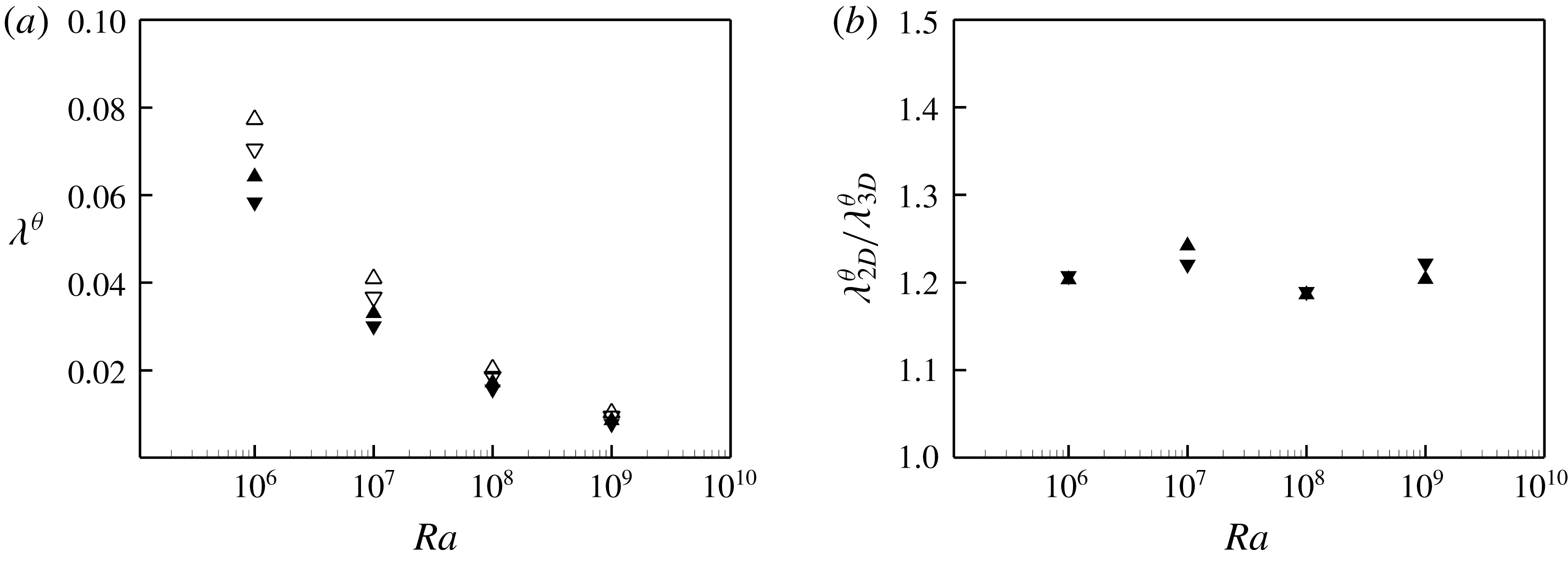
increases. This is clearly shown in figure 11(a), where
 $\unicode[STIX]{x1D706}_{t}^{\unicode[STIX]{x1D703}}$
and
 $\unicode[STIX]{x1D706}_{b}^{\unicode[STIX]{x1D703}}$
are found to decrease by almost an order of magnitude from
 $Ra=10^{6}$
to
 $10^{9}$
. Moreover, the 2-D predictions are substantially larger than the 3-D ones, an effect that is attributed to the larger temperature gradients on the walls for the 3-D cases, shown in table 3. The variation of
 $\unicode[STIX]{x1D706}_{2D}^{\unicode[STIX]{x1D703}}/\unicode[STIX]{x1D706}_{3D}^{\unicode[STIX]{x1D703}}$
as a function of
 $Ra$
is shown in figure 11(b) and reveals that this ratio is almost insensitive to the increase of
 $Ra$
, for both BLs. The scaling relations of the thermal BL thicknesses were calculated using a least-squares fit on a classic power law and are listed in table 4. Since the results do not exhibit a top–bottom symmetry, a distinction is made between the top and the bottom BLs. The scaling exponent remains almost unaffected for the 2-D and 3-D cases and also for the top and the bottom BLs. Additionally, the scaling exponent is very similar to the OB results reported by Wang & Xia (Reference Wang and Xia2003). This finding suggests that the scaling exponents are only weakly affected by the NOB character of the flow, similar to the Nusselt number scaling.
(a) Variation of thermal BL thickness
 $\unicode[STIX]{x1D706}^{\unicode[STIX]{x1D703}}$
with
 $Ra$
for
 $\unicode[STIX]{x0394}T=40~\text{K}$
: open upward pointing triangles,
 $\unicode[STIX]{x1D706}_{t}^{\unicode[STIX]{x1D703}}$
– two dimensions; open downward pointing triangles,
 $\unicode[STIX]{x1D706}_{b}^{\unicode[STIX]{x1D703}}$
– two dimensions; solid upward pointing triangles,
 $\unicode[STIX]{x1D706}_{t}^{\unicode[STIX]{x1D703}}$
– three dimensions; solid downward pointing triangles,
 $\unicode[STIX]{x1D706}_{b}^{\unicode[STIX]{x1D703}}$
– three dimensions. (b) Variation of
 $\unicode[STIX]{x1D706}_{2D}^{\unicode[STIX]{x1D703}}/\unicode[STIX]{x1D706}_{3D}^{\unicode[STIX]{x1D703}}$
with
 $Ra$
for
 $\unicode[STIX]{x0394}T=40~\text{K}$
: downward pointing triangles, bottom BL; upward pointing triangles, top BL.
Scaling of thermal BL thickness
 $\unicode[STIX]{x1D706}^{\unicode[STIX]{x1D703}}$
at the top and the bottom of the cavity for both the 2-D and the 3-D cases, at
 $\unicode[STIX]{x0394}T=40~\text{K}$
. The power laws were calculated using the least-squares method.

Figure 12 presents the influence of
 $\unicode[STIX]{x0394}T$
on
 $\unicode[STIX]{x1D706}_{t}^{\unicode[STIX]{x1D703}}$
and
 $\unicode[STIX]{x1D706}_{b}^{\unicode[STIX]{x1D703}}$
for
 $Ra=10^{9}$
. As
 $\unicode[STIX]{x0394}T$
increases, the top thermal BL thickens while the bottom one becomes thinner, in both the 2-D and 3-D cases. Additionally,
 $\unicode[STIX]{x1D706}_{t}^{\unicode[STIX]{x1D703}}$
is consistently larger than
 $\unicode[STIX]{x1D706}_{b}^{\unicode[STIX]{x1D703}}$
for both the 2-D and 3-D sets of simulations. This can be rationalised following the definition of
 $\unicode[STIX]{x1D706}^{\unicode[STIX]{x1D703}}$
in (2.10). More specifically, even though both the average temperature gradient along the top wall (table 3) and
 $\unicode[STIX]{x1D6E5}_{t}$
(figure 10) are increased,
 $\unicode[STIX]{x1D6E5}$
exhibits a stronger temperature dependence which leads to the thicker thermal BLs at the top of the cavity, compared to the bottom. The ratio of the thermal BL thicknesses predicted by 2-D and 3-D simulations
 $\unicode[STIX]{x1D706}_{2D}^{\unicode[STIX]{x1D703}}/\unicode[STIX]{x1D706}_{3D}^{\unicode[STIX]{x1D703}}$
is presented in figure 12(b). This ratio exhibits only a weak dependence on
 $\unicode[STIX]{x0394}T$
, acquiring an almost constant value of approximately
 $1.20$
.
Variation of (a) thermal BL thickness
 $\unicode[STIX]{x1D706}^{\unicode[STIX]{x1D703}}$
and (b)
 $\unicode[STIX]{x1D706}_{2D}^{\unicode[STIX]{x1D703}}/\unicode[STIX]{x1D706}_{3D}^{\unicode[STIX]{x1D703}}$
with
 $\unicode[STIX]{x0394}T$
for
 $Ra=10^{9}$
. The notation is the same as in figure 11.

The NOB effects on the thermal BLs can be better quantified using the ratio
 $\unicode[STIX]{x1D706}_{NOB}^{\unicode[STIX]{x1D703}}/\unicode[STIX]{x1D706}_{OB}^{\unicode[STIX]{x1D703}}$
. Figure 13 shows that this ratio depends mainly on
 $\unicode[STIX]{x0394}T$
and is almost unaffected by the variation of
 $Ra$
. Additionally, some differences between 2-D and 3-D simulations are visible, more prominently for the top BL. The 2-D predictions fluctuate more intensely with
 $Ra$
, compared to the 3-D predictions that remain relatively unaffected. As a function of
 $\unicode[STIX]{x0394}T$
, the 2-D ratio at the top BL exhibits a weaker increase compared to the 3-D cases. For both the 2-D and 3-D predictions, the ratio at the bottom BL exhibits a steeper descent than the ascent at the top BL.
Variation of
 $\unicode[STIX]{x1D706}_{NOB}^{\unicode[STIX]{x1D703}}/\unicode[STIX]{x1D706}_{OB}^{\unicode[STIX]{x1D703}}$
as a function of (a)
 $Ra$
for
 $\unicode[STIX]{x0394}T=40~\text{K}$
and (b)
 $\unicode[STIX]{x0394}T$
for
 $Ra=10^{9}$
: open upward pointing triangles, top BL – two dimensions; open downward pointing triangles, bottom BL – two dimensions; solid upward pointing triangles, top BL – three dimensions; solid downward pointing triangles, bottom BL – three dimensions; diamonds, 3-D numerical results in a cylindrical domain at
 $Ra=10^{9}$
reported by Horn & Shishkina (Reference Horn and Shishkina2014).

5 Profiles of the near-wall temperature statistics
In this section, the near-wall vertical distributions of the space-averaged mean and r.m.s. values of temperature are presented to investigate the modifications stemming from the property variations. Since the objective is to reveal previously unexplored NOB effects and not to compare the 2-D and 3-D solutions, this section focuses exclusively on 3-D results. Figure 14(a,b) shows the near-wall vertical distributions of
 $\langle \unicode[STIX]{x1D6E9}\rangle _{t,x,y}$
for various
 $Ra$
values, at
 $\unicode[STIX]{x0394}T=40~\text{K}$
. As expected, the increase of
 $Ra$
is accompanied by sharper temperature gradients close to the walls. Moreover, the temperature gradient on the top wall is consistently larger than the corresponding one at the bottom wall. The actual values of the temperature gradients are listed in table 3, where the values on the top wall are approximately 9 % increased compared to the values on the bottom wall in every 3-D case. This asymmetry can be attributed to the variation of the thermal conductivity of water which increases with temperature. Further away from the walls, the averaged temperature reaches a plateau value which varies only weakly with
 $Ra$
, as demonstrated by the values of the centre temperature
 $\unicode[STIX]{x1D6E9}_{c}$
in figure 9(a).
Effect of
 $Ra$
on the vertical distribution of the plane-averaged mean temperature
 $\langle \unicode[STIX]{x1D6E9}\rangle _{t,x,y}$
(a,b) and r.m.s. values of temperature
 $\langle \unicode[STIX]{x1D6E9}_{rms}\rangle _{x,y}$
(c,d) in the vicinity of the bottom (a,c) and the top (b,d) walls: solid line,
 $Ra=10^{6}$
; dashed line,
 $Ra=10^{7}$
; dashed-dotted line,
 $Ra=10^{8}$
; dashed-dotted-dotted line,
 $Ra=10^{9}$
. In all cases
 $\unicode[STIX]{x0394}T=40~\text{K}$
.

The effect of
 $Ra$
on the near-wall vertical distributions of
 $\langle \unicode[STIX]{x1D6E9}_{rms}\rangle _{x,y}$
is shown in figure 14(c,d), for
 $\unicode[STIX]{x0394}T=40~\text{K}$
. All profiles exhibit a sharp increase near the walls, before reaching a maximum and decrease towards the core of the cavity. The maximum r.m.s. values decrease weakly and monotonically with
 $Ra$
, something that was also observed in the OB study of Du Puits et al. (Reference Du Puits, Resagk, Tilgner, Busse and Thess2007), albeit for a lower Prandtl number. At the top of the cavity, the maximum values are consistently larger compared to the bottom of the cavity, owing to the smaller thermal diffusivity of water at the top (colder) part of the cavity. More specifically, larger thermal diffusivity values redistribute temperature inhomogeneities more effectively, reducing the fluctuations of the temperature field in this region.
Figure 15(a,b) shows the effect of
 $\unicode[STIX]{x0394}T$
on the near-wall vertical distributions of
 $\langle \unicode[STIX]{x1D6E9}\rangle _{t,x,y}$
, at
 $Ra=10^{9}$
. In all cases, a linear region is detected next to the horizontal walls which corresponds to the viscous sublayer. The thickness of this linear layer is affected by
 $\unicode[STIX]{x0394}T$
, although the temperature gradient in this layer is almost unaffected. More specifically, as
 $\unicode[STIX]{x0394}T$
increases this linear region shrinks at the bottom and expands at the top of the cavity. Additionally, the temperature plateau outside the thermal BLs is shifted to higher values, in accordance to the
 $\unicode[STIX]{x1D6E9}_{c}$
variation with
 $\unicode[STIX]{x0394}T$
, shown in figure 9(b).
Effect of
 $\unicode[STIX]{x0394}T$
on the vertical distribution of the plane-averaged mean temperature
 $\langle \unicode[STIX]{x1D6E9}\rangle _{t,x,y}$
(a,b) and r.m.s. values of temperature
 $\langle \unicode[STIX]{x1D6E9}_{rms}\rangle _{x,y}$
(c,d) in the vicinity of the bottom (a,c) and the top (b,d) walls: solid line, OB; dashed line,
 $\unicode[STIX]{x0394}T=20~\text{K}$
; dashed-dotted line,
 $\unicode[STIX]{x0394}T=40~\text{K}$
; dashed-dotted-dotted line,
 $\unicode[STIX]{x0394}T=60~\text{K}$
. In all cases
 $Ra=10^{9}$
.

Figure 15(c,d) reveals the effects of
 $\unicode[STIX]{x0394}T$
on the near-wall vertical distributions of
 $\langle \unicode[STIX]{x1D6E9}_{rms}\rangle _{x,y}$
. As
 $\unicode[STIX]{x0394}T$
increases, the value of the maximum in the vicinity of the top wall increases and its location moves away from the wall. The opposite effect is observed at the bottom of the cavity, i.e. the maximum decreases and moves closer to the bottom wall. More specifically, the comparison of the NOB results with
 $\unicode[STIX]{x0394}T=60~\text{K}$
against the OB results reveals an increase of the maximum r.m.s. value at the top of the cavity by
 $11.7\,\%$
and a decrease at the bottom of the cavity by
 $8.5\,\%$
. The distance from the wall to the location where the r.m.s. values reach their maximum (
 $\unicode[STIX]{x1D706}^{rms}$
), can be considered as an alternative definition of the thermal BL thickness (Tilgner, Belmonte & Libchaber Reference Tilgner, Belmonte and Libchaber1993). Moreover, higher statistical moments were shown to exhibit different properties below and above this thickness, suggesting that
 $\unicode[STIX]{x1D706}^{rms}$
should be preferred over
 $\unicode[STIX]{x1D706}^{\unicode[STIX]{x1D6E9}}$
as a natural length scale for the thermal BLs (Zhou & Xia Reference Zhou and Xia2013). Table 5 presents the ratio
 $\unicode[STIX]{x1D706}^{rms}/\unicode[STIX]{x1D706}^{\unicode[STIX]{x1D6E9}}$
at
 $Ra=10^{9}$
for different values of
 $\unicode[STIX]{x0394}T$
. In all cases
 $\unicode[STIX]{x1D706}^{rms}/\unicode[STIX]{x1D706}^{\unicode[STIX]{x1D6E9}}<1$
, meaning that the position of the r.m.s. maximum is located inside the thermal BL. This ratio exhibits similar values at the top and at the bottom of the cavity, with no systematic dependence on
 $\unicode[STIX]{x0394}T$
.
Ratio
 $\unicode[STIX]{x1D706}^{rms}/\unicode[STIX]{x1D706}^{\unicode[STIX]{x1D6E9}}$
at
 $Ra=10^{9}$
, for different values of
 $\unicode[STIX]{x0394}T$
.

6 Summary and conclusions
Rayleigh–Bénard convection in water was studied by means of DNS, taking into account the variation of properties with temperature. The simulations were carried out in a cavity with a rectangular cross-section, for Rayleigh numbers in the range of
 $10^{6}\leqslant Ra\leqslant 10^{9}$
with temperature differences up to 60 K.
One of the main objectives of the present work was to quantify NOB effects using 2-D and 3-D simulations and perform comparisons. A reasonable agreement was observed between 2-D and 3-D results for the centre temperature and temperature drop inside the thermal BLs. On the other hand, the predicted Nusselt numbers and thermal BL thicknesses exhibited significant deviations. More specifically, these parameters were found to deviate by as much as
 $20\,\%$
when computed using 2-D and 3-D simulations. Nonetheless, when these output parameters were normalised with the respective OB values, the agreement improved. Moreover, the LSC roll was found to shift its orientation from the
 $x$
–
 $z$
plane in the 2-D cases to the
 $y$
–
 $z$
plane in the 3-D cases. The quantification of the LSC shape and structure also revealed significant differences which were linked to the differences in the predicted output parameters.
Another focus of this study was to identify how the NOB effects modify the mean and r.m.s. distributions of the temperature field, leading to the breaking of the top–bottom symmetry. As
 $\unicode[STIX]{x0394}T$
increased, the near-wall linear part of the mean temperature distribution expanded at the top and contracted at the bottom of the cavity, while the value of the mean temperature in the bulk region increased. Moreover, the near-wall maximum values of the temperature r.m.s. increased in the vicinity of the top wall and decreased next to the bottom wall. Likewise, the locations of the near-wall maxima were found to shift away from the top wall and move closer to the bottom wall.
Up to
 $Ra=10^{9}$
, the NOB effects were found to depend only weakly on
 $Ra$
. The extrapolation of these results to higher
 $Ra$
values needs further justification because of the expected transition to turbulence of the boundary layers at around
 $Ra>10^{13}$
, signalling the transition to the ultimate regime (Grossmann & Lohse Reference Grossmann and Lohse2000, Reference Grossmann and Lohse2001). An interesting future extension of the present study would be to simulate flows at even higher Rayleigh numbers, as close to the ultimate regime as possible. At such high Rayleigh numbers, it would be possible to distinguish the BL modifications that are induced by the NOB effects and those that emerge from the ultimate regime.
Acknowledgements
The authors would like to thank the Cyprus State Scholarship Foundation who financed and supported this research.