1 Introduction
The flow of granular material constitutes an everyday occurrence which plays a fundamental role in both industry and the natural world. A comprehensive understanding of the behaviour of such material is essential for the mitigation of risks posed to both infrastructure and populations by destructive geophysical flows, such as debris avalanches and pyroclastic flows (Delannay et al. Reference Delannay, Valance, Mangeney, Roche and Richard2017). Moreover in industrial settings, the pharmaceutical, food manufacturing and mining sectors rely heavily on the handling and processing of granular material on a daily basis (Jaeger, Nagel & Behringer Reference Jaeger, Nagel and Behringer1996; Barker & Gray Reference Barker and Gray2017). As such, given its ubiquity in many sectors of society, the flow of granular material has been the subject of intensive research activity. For example, phenomena such as avalanching (Daerr Reference Daerr2001; Gray, Tai & Noelle Reference Gray, Tai and Noelle2003; Baker, Barker & Gray Reference Baker, Barker and Gray2016a ) and particle-size segregation (Gray Reference Gray2001; Pihler-Puzović & Mullin Reference Pihler-Puzović and Mullin2013; Gray, Gajjar & Kokelaar Reference Gray, Gajjar and Kokelaar2015) have attracted much attention, and the determination of a suitable rheology for granular material has been extensively studied (Pouliquen Reference Pouliquen1999; MiDi Reference Midi2004; Da Cruz et al. Reference Da Cruz, Emam, Prochnow, Roux and Chevoir2005; Jop, Forterre & Pouliquen Reference Jop, Forterre and Pouliquen2005; Koval et al. Reference Koval, Roux, Corfdir and Chevoir2009). However, the mathematical modelling of the flow of granular material represents a major challenge, and a universally accepted model for the description of such flows, even in relatively simple geometries, has remained elusive (Jop Reference Jop2015).
Depending on the rate of deformation, granular flows are often classified according to three regimes: (i) a quasi-static regime in which particle interaction is dominated by enduring frictional contacts, (ii) a gaseous regime in which binary collisions are dominant and (iii) a dense inertial (commonly known as liquid) regime where both frictional contacts and collisions persist (Da Cruz et al.
Reference Da Cruz, Emam, Prochnow, Roux and Chevoir2005; Forterre & Pouliquen Reference Forterre and Pouliquen2008; Jop Reference Jop2015). This liquid phase is the most frequently encountered regime in practical applications (Forterre & Pouliquen Reference Forterre and Pouliquen2008). The recent development of the incompressible inertial-dependent rheology (IIDR) has had a significant impact on the continuum modelling of granular flows of this type (Gray & Edwards Reference Gray and Edwards2014). This rheology relates the effective friction coefficient,
 $\unicode[STIX]{x1D707}$
, to a dimensionless variable,
 $I$
, known as the inertial number, which represents the ratio of representative time scales for microscopic and macroscopic deformation in the flow, and has hence become known as the
 $\unicode[STIX]{x1D707}(I)$
rheology.
The
 $\unicode[STIX]{x1D707}(I)$
functional dependence was originally proposed by MiDi (Reference Midi2004) by considering the dimensional analysis of a simple shear flow, and has been investigated using numerical and experimental data in shear (Da Cruz et al.
Reference Da Cruz, Emam, Prochnow, Roux and Chevoir2005) and chute flow geometries (Pouliquen Reference Pouliquen1999). In particular Jop et al. (Reference Jop, Forterre and Pouliquen2005) inferred a widely used form for
 $\unicode[STIX]{x1D707}(I)$
from the chute flow data of Pouliquen & Forterre (Reference Pouliquen and Forterre2002), which was subsequently used in the tensorial generalisation of the scalar rheology proposed by Jop, Forterre & Pouliquen (Reference Jop, Forterre and Pouliquen2006). This leads to a model which is more or less identical to the incompressible Navier–Stokes equations, except for a viscosity which is now dependent on pressure and strain rate. Such a model is amenable to numerical simulation given that existing incompressible flow solvers can readily be adapted for variable viscosity. Indeed the rheology has proved successful in describing the bulk characteristics of shear and chute flows (MiDi Reference Midi2004), three-dimensional flow on a pile (Jop et al.
Reference Jop, Forterre and Pouliquen2006) and on an incline (Baker et al.
Reference Baker, Barker and Gray2016a
), the formation of erosion deposition waves (Gray & Edwards Reference Gray and Edwards2014; Edwards & Gray Reference Edwards and Gray2015) and segregation-induced finger formation (Baker, Johnson & Gray Reference Baker, Johnson and Gray2016b
).
Despite these successes, Barker et al. (Reference Barker, Schaeffer, Bohorquez and Gray2015) have demonstrated that the IIDR model is linearly ill-posed at low and high inertial numbers, i.e. small-wavelength perturbations to the system grow without bound as their wavelength tends to zero. While in certain cases this short-wavelength instability can be quenched by Kelvin wavevector stretching at large times (Goddard & Lee Reference Goddard and Lee2017), in general it leads to grid-dependent numerical simulations (Woodhouse et al.
Reference Woodhouse, Thornton, Johnson, Kokelaar and Gray2012) and is typically associated with the omission of important physical processes from the model (Fowler Reference Fowler1997, p. 280). Although the recent work of Goddard & Lee (Reference Goddard and Lee2018) illustrates that linear ill-posedness can be eliminated in strongly dissipative incompressible models, the inclusion of compressibility seems to provide a natural, physically motivated remedy to this ill-posedness, as demonstrated independently by Barker et al. (Reference Barker, Schaeffer, Shearer and Gray2017) and Heyman et al. (Reference Heyman, Delannay, Tabuteau and Valance2017), while also incorporating additional physics into the model. In particular, borrowing ideas from critical-state soil mechanics to postulate an additional constitutive equation, Barker et al. (Reference Barker, Schaeffer, Shearer and Gray2017) have proposed the compressible
 $I$
-dependent rheology (CIDR) for dense granular flow.
This model constitutes a linearly well-posed hydrodynamical description of the granular medium which also allows for dilation/compaction. The incorporation of compressibility may enable application of the CIDR model to cases in which solid fraction fluctuations are thought to be particularly important, and hence where the incompressibility assumption of the IIDR model is invalid, e.g. acoustic waves in shear flow (Trulsson et al. Reference Trulsson, Bouzid, Claudin and Andreotti2013), the formation of complex internal structures in high-speed inclined flows (Brodu et al. Reference Brodu, Delannay, Valance and Richard2015) and immersed flows (Jop Reference Jop2015). However the simulation of such flows represents a significant challenge given that most existing fluid flow solvers are not easily adapted to incorporate compressibility, and indeed this has motivated Barker & Gray (Reference Barker and Gray2017) to consider regularising the IIDR model by using alternative functional forms for the effective friction coefficient. Thus, before formulating numerical methods to simulate this compressible flow with variable viscosity, one is naturally motivated to consider the veracity of the CIDR model for simple flow geometries and to investigate whether its additional complexity yields predictions which more accurately capture experimental results. In this paper, we investigate the efficacy of the CIDR model in predicting granular instability properties observed in two disparate geometries: inclined plane flow (Forterre & Pouliquen Reference Forterre and Pouliquen2003) and plane shear in the absence of gravity (Trulsson et al. Reference Trulsson, Bouzid, Claudin and Andreotti2013).
Steady uniform flow of a granular material on a rough inclined plane is found to be unstable to small-amplitude perturbations, and this instability can lead to the formation of granular roll waves on the free surface which are analogous in form to those found for water flow down a steep incline (see Fowler Reference Fowler2011, p. 238). Forterre & Pouliquen (Reference Forterre and Pouliquen2003) performed an experimental analysis of this long-surface-wave instability for glass beads and sand, and illustrated that it is attributable to the classic inertial instability frequently encountered in hydrodynamics (e.g. Drazin & Reid Reference Drazin and Reid1981, chap. 1), which should not be confused with short-wave instability resulting from ill-posedness. By investigating the downstream evolution of sinusoidal perturbations to the chute flow surface as a function of the perturbation frequency, the authors determined the dispersion relation relating the perturbation growth rate to the forcing frequency in the linear growth regime, and, in turn, calculated the frequency beyond which the system is stable as a function of the Froude number.
For the case of two-dimensional plane shear in the absence of gravity, Trulsson et al. (Reference Trulsson, Bouzid, Claudin and Andreotti2013) have demonstrated by means of discrete element simulations the emergence of spontaneous oscillations in the system at a well-defined angular frequency, which the authors attribute to a dynamic compressibility. By considering the velocity response to linear forcing both parallel and transverse to the direction of shearing, they find that this response presents a resonance whose frequency coincides with that of the spontaneous oscillations and is independent of the restitution coefficient and spring constant characterising the granular medium. The prediction of both these shear and chute flow instabilities constitutes two non-trivial test cases for the CIDR model. Indeed, chute flow instability has previously been used to examine the predictive capability of the IIDR model (Forterre Reference Forterre2006) and a depth-averaged version of the same (Gray & Edwards Reference Gray and Edwards2014).
Although the CIDR model represents a promising step forward in the continuum modelling of granular material, one must also be cognisant of its limitations. Indeed, its current formulation has recently been criticised by Goddard & Lee (Reference Goddard and Lee2018) who raise concerns regarding the possible elimination of yield stress and the loss of material frame-indifference in the model (see §§ 2 and 3, respectively, for additional discussion). Moreover, the inclusion of compressibility alone does not provide a remedy to all existing limitations of the
 $\unicode[STIX]{x1D707}(I)$
rheology, which is itself phenomenological in nature with little relation to the microstructure of the granular medium. One particular problem relates to modelling the transition from the dense inertial regime (characterised by
 $0.01<I<0.5$
(Jop Reference Jop2015)), for which the rheology was initially proposed (Jop et al.
Reference Jop, Forterre and Pouliquen2006), to the quasi-static regime. For example, the phenomenon of rate-independent shear bands, as described by Mueth et al. (Reference Mueth, Debregeas, Karczmar, Eng, Nagel and Jaeger2000) and Fenistein & van Hecke (Reference Fenistein and van Hecke2003), is not captured by the
 $\unicode[STIX]{x1D707}(I)$
rheology.
While continuum modelling has attracted significant interest in recent decades, several alternative modelling approaches for granular flow have also been developed, including those based on microstructural (Sun & Sundaresan Reference Sun and Sundaresan2011) and Cosserat theories (Tejchman & Gudehus Reference Tejchman and Gudehus2001). For rapid granular flows, kinetic theories which describe the evolution of the mean density, velocity and granular temperature (related to the velocity fluctuations) in the system have been developed (Jenkins & Savage Reference Jenkins and Savage1983). Such models have been successfully applied to instability phenomena observed in both chute and Couette flow geometries (Forterre & Pouliquen Reference Forterre and Pouliquen2002; Alam et al. Reference Alam, Arakeri, Nott, Goddard and Herrmann2005), and indeed have been extended to the dense flow regime (Berzi & Jenkins Reference Berzi and Jenkins2015). A number of non-local rheologies have also been proposed in recent years (Pouliquen & Forterre Reference Pouliquen and Forterre2009; Kamrin & Koval Reference Kamrin and Koval2012; Bouzid et al. Reference Bouzid, Trulsson, Claudin, Clément and Andreotti2013) which attempt to account for observed quasi-static flow discrepancies, and the incorporation of such a rheology may form a natural extension to the current CIDR formulation. In our work, however, we concern ourselves with the application of the CIDR model to dense inertial flows of interest, and thus such extensions fall beyond the scope of this work.
The remainder of this paper is structured as follows. The CIDR model, which we modify slightly from its original formulation, is outlined in detail in § 2 for a general Cartesian geometry. We then restrict our interest to inclined plane flow in § 3, where we non-dimensionalise the model and describe the steady uniform flow. A full stability analysis for this flow is carried out in § 3.2, where we also describe a Chebyshev collocation method to solve the resulting eigenvalue problem and validate its accuracy against the incompressible results of Forterre (Reference Forterre2006). Stability results are presented in § 3.5 where it is shown that the CIDR model predictions both quantitatively match the experimental results of Forterre & Pouliquen (Reference Forterre and Pouliquen2003) and indeed better those of the IIDR model. In an analogous manner, we proceed to our analysis of the plane shear geometry in § 4, where we also briefly discuss an alternative compressible flow model presented by Trulsson et al. (Reference Trulsson, Bouzid, Claudin and Andreotti2013). The subsequent stability predictions are outlined in § 4.4, where we demonstrate that the CIDR model can qualitatively capture the instability behaviour observed in the discrete element simulations of Trulsson et al. (Reference Trulsson, Bouzid, Claudin and Andreotti2013).
2 Governing equations
We first present the model equations for dense granular flow in a general Cartesian geometry before restricting our interest to the inclined plane and plane shear geometries discussed in §§ 3 and 4, respectively. Both flows are quasi-two-dimensional in nature and hence we neglect cross-stream variations and assume zero velocity in this direction. Taking particles of constant density
 $\unicode[STIX]{x1D70C}_{s}$
, the granular fluid is characterised by a velocity field denoted
 $\boldsymbol{u}=(u,0,v)$
in the
 $(x,y,z)$
directions (henceforth referred to as the downstream, cross-stream and normal directions, respectively) and a variable solids volume fraction,
 $\unicode[STIX]{x1D719}$
. The flow is described using the CIDR model presented in Barker et al. (Reference Barker, Schaeffer, Shearer and Gray2017), to which the reader is referred for more information, which we modify slightly to account for the influence of cross-stream stresses on the plane flow.
In the CIDR model,
 $\unicode[STIX]{x1D719}$
is considered a dynamic variable as opposed to being assumed constant or a ‘slaved variable’ of
 $I$
(Pouliquen et al.
Reference Pouliquen, Cassar, Jop, Forterre and Nicolas2006; Pouliquen & Forterre Reference Pouliquen and Forterre2009). Thus, conservation of mass of the granular medium takes the form
 $$\begin{eqnarray}\displaystyle \frac{\unicode[STIX]{x2202}\unicode[STIX]{x1D719}}{\unicode[STIX]{x2202}t}+\unicode[STIX]{x1D735}\boldsymbol{\cdot }(\unicode[STIX]{x1D719}\boldsymbol{u})=0, & & \displaystyle\end{eqnarray}$$
from which the incompressibility constraint
 $\unicode[STIX]{x1D735}\boldsymbol{\cdot }\boldsymbol{u}=0$
, assumed in the IIDR model (Jop et al.
Reference Jop, Forterre and Pouliquen2006), follows for constant
 $\unicode[STIX]{x1D719}$
. Conservation of momentum is given by
 $$\begin{eqnarray}\displaystyle \unicode[STIX]{x1D70C}_{s}\unicode[STIX]{x1D719}\left(\frac{\unicode[STIX]{x2202}\boldsymbol{u}}{\unicode[STIX]{x2202}t}+(\boldsymbol{u}\boldsymbol{\cdot }\unicode[STIX]{x1D735})\boldsymbol{u}\right)=\unicode[STIX]{x1D735}\boldsymbol{\cdot }\unicode[STIX]{x1D748}+\unicode[STIX]{x1D70C}_{s}\unicode[STIX]{x1D719}\boldsymbol{g}, & & \displaystyle\end{eqnarray}$$
where
 $\boldsymbol{g}$
is acceleration due to gravity. The Cauchy stress tensor
 $\unicode[STIX]{x1D748}$
can be decomposed into its pressure
 $p$
and deviatoric stress
 $\unicode[STIX]{x1D749}$
contributions, i.e.
 $$\begin{eqnarray}\displaystyle \unicode[STIX]{x1D748}=-p\unicode[STIX]{x1D739}+\unicode[STIX]{x1D749}, & & \displaystyle\end{eqnarray}$$
where
 $\unicode[STIX]{x1D739}$
is the
 $3\times 3$
identity tensor. In the CIDR model, closure of this system is achieved by specifying three constitutive equations for stress–strain rate alignment, shear stress and the solid fraction. The alignment condition between the deviatoric stress tensor and the deviatoric strain rate tensor
 $\unicode[STIX]{x1D63F}$
is given by
 $$\begin{eqnarray}\displaystyle \frac{\unicode[STIX]{x1D749}}{\Vert \unicode[STIX]{x1D749}\Vert }=\frac{\unicode[STIX]{x1D63F}}{\Vert \unicode[STIX]{x1D63F}\Vert },\quad \unicode[STIX]{x1D60B}_{ij}=\frac{1}{2}\left(\frac{\unicode[STIX]{x2202}u_{i}}{\unicode[STIX]{x2202}x_{j}}+\frac{\unicode[STIX]{x2202}u_{j}}{\unicode[STIX]{x2202}x_{i}}\right)-\frac{(\unicode[STIX]{x1D735}\boldsymbol{\cdot }\boldsymbol{u})}{3}\unicode[STIX]{x03B4}_{ij}\quad i,j=1,2,3, & & \displaystyle\end{eqnarray}$$
where
 $\Vert \unicode[STIX]{x1D63F}\Vert =\sqrt{\unicode[STIX]{x1D60B}_{ij}\unicode[STIX]{x1D60B}_{ij}/2}$
is the second invariant (the Einstein summation convention is assumed). Note that in (2.4) we consider the three-dimensional deviatoric strain rate tensor (
 $-1/3$
in the divergence term) as opposed to its two-dimensional form (with
 $-1/2$
) given by (2.7) of Barker et al. (Reference Barker, Schaeffer, Shearer and Gray2017). This accounts for the fact that a non-zero stress field in the cross-stream direction can exist in tandem with a zero velocity component. Although a two-dimensional flow is considered here, the governing equations are three-dimensional in nature and hence this reduction in dimensionality should not change the stress tensor formulation. We anticipate that this modification does not impact on the linear well-posedness of the model.
The second constitutive equation takes the form of a generalised yield condition which relates the shear stress
 $\unicode[STIX]{x03C4}=\Vert \unicode[STIX]{x1D749}\Vert$
in the flowing medium to the pressure, solid fraction and inertial number, i.e.
 $$\begin{eqnarray}\displaystyle \unicode[STIX]{x03C4}=Y(p,\unicode[STIX]{x1D719},I), & & \displaystyle\end{eqnarray}$$
where
 $I$
is given by (Jop et al.
Reference Jop, Forterre and Pouliquen2006)
 $$\begin{eqnarray}\displaystyle I=\frac{2\Vert \unicode[STIX]{x1D63F}\Vert d}{\sqrt{p/\unicode[STIX]{x1D70C}_{s}}}, & & \displaystyle\end{eqnarray}$$
with
 $d$
the particle diameter. For the final constitutive condition, Barker et al. (Reference Barker, Schaeffer, Shearer and Gray2017) suggest a generalised flow rule which allows for dilation/compaction of the medium
 $$\begin{eqnarray}\displaystyle \unicode[STIX]{x1D735}\boldsymbol{\cdot }\boldsymbol{u}=2f(p,\unicode[STIX]{x1D719},I)\Vert \unicode[STIX]{x1D63F}\Vert . & & \displaystyle\end{eqnarray}$$
Note that constant
 $\unicode[STIX]{x1D719}$
represents the equivalent condition in the IIDR model. Equations (2.1)–(2.7) constitute a closed, linearly well-posed system provided that the functions
 $Y$
and
 $f$
satisfy a number of conditions (see Barker et al.
Reference Barker, Schaeffer, Shearer and Gray2017, (2.19) and (2.20)). Throughout this work, we assume the forms as detailed in Barker et al. (Reference Barker, Schaeffer, Shearer and Gray2017), i.e.
 $$\begin{eqnarray}\displaystyle Y=\unicode[STIX]{x1D6FC}(I)p-\frac{p^{2}}{C(\unicode[STIX]{x1D719})},\quad f=\unicode[STIX]{x1D6FD}(I)-\frac{2p}{C(\unicode[STIX]{x1D719})}, & & \displaystyle\end{eqnarray}$$
where
 $$\begin{eqnarray}\displaystyle & \displaystyle \unicode[STIX]{x1D6FC}(I)=\frac{4\unicode[STIX]{x1D707}(I)}{5}+\frac{12}{25}\int _{0}^{1}s^{-3/5}\unicode[STIX]{x1D707}(sI)\,\text{d}s, & \displaystyle\end{eqnarray}$$
 $$\begin{eqnarray}\displaystyle & \displaystyle \unicode[STIX]{x1D6FD}(I)=-\frac{2\unicode[STIX]{x1D707}(I)}{5}+\frac{24}{25}\int _{0}^{1}s^{-3/5}\unicode[STIX]{x1D707}(sI)\,\text{d}s, & \displaystyle\end{eqnarray}$$
 $$\begin{eqnarray}\displaystyle & \displaystyle \unicode[STIX]{x1D707}(I)=\unicode[STIX]{x1D707}_{1}+I\left(\frac{\unicode[STIX]{x1D707}_{2}-\unicode[STIX]{x1D707}_{1}}{I_{0}+I}\right) & \displaystyle\end{eqnarray}$$
 $$\begin{eqnarray}\displaystyle C(\unicode[STIX]{x1D719})=\frac{{\mathcal{P}}}{b}{\hat{C}}(\unicode[STIX]{x1D713}),\quad {\hat{C}}(\unicode[STIX]{x1D713})=\frac{\unicode[STIX]{x1D713}}{1-\unicode[STIX]{x1D713}},\quad \unicode[STIX]{x1D713}=\frac{\unicode[STIX]{x1D719}-\unicode[STIX]{x1D719}_{min}}{\unicode[STIX]{x1D719}_{max}-\unicode[STIX]{x1D719}_{min}}, & & \displaystyle\end{eqnarray}$$
where
 $b$
is a non-dimensional parameter and
 ${\mathcal{P}}$
denotes a suitable pressure scaling for the function
 $C$
, as required from consideration of the constitutive laws (2.8).
Barker et al. (Reference Barker, Schaeffer, Shearer and Gray2017) propose the ansatz (2.8) in analogy with similar constitutive equations used in critical-state soil mechanics, in which the dilatancy function in (2.7) is given by the slope of the yield function for fixed
 $\unicode[STIX]{x1D719}$
(e.g. see Jackson Reference Jackson and Meyer1983). This in particular motivates the definition of
 $f$
in (2.8), while the specific form for
 $Y$
is chosen such that, when deformation occurs without any associated change in
 $\unicode[STIX]{x1D719}$
, the yield condition reduces to the standard
 $\unicode[STIX]{x1D707}(I)$
-type rheology, i.e.
 $Y=[\unicode[STIX]{x1D6FC}(I)-\unicode[STIX]{x1D6FD}(I)/2]p$
. In this constant
 $\unicode[STIX]{x1D719}$
case, it is reasonable to suppose that the CIDR equations reduce to the IIDR model given its previous success. Under this assumption, specification of the functional forms for
 $\unicode[STIX]{x1D6FC}(I)$
and
 $\unicode[STIX]{x1D6FD}(I)$
in (2.9) follows from
 $$\begin{eqnarray}\displaystyle \unicode[STIX]{x1D707}(I)=\unicode[STIX]{x1D6FC}(I)-\frac{\unicode[STIX]{x1D6FD}(I)}{2},\quad \frac{\unicode[STIX]{x2202}Y}{\unicode[STIX]{x2202}p}-\frac{I}{2p}\frac{\unicode[STIX]{x2202}Y}{\unicode[STIX]{x2202}I}=f+I\frac{\unicode[STIX]{x2202}f}{\unicode[STIX]{x2202}I}, & & \displaystyle\end{eqnarray}$$
where (2.11b
) represents hypothesis (2.19) of Barker et al. (Reference Barker, Schaeffer, Shearer and Gray2017), required for the model to be linearly well-posed. The rheology (2.9c
) originally proposed by Jop et al. (Reference Jop, Forterre and Pouliquen2005) is assumed, where
 $\unicode[STIX]{x1D707}_{2}>\unicode[STIX]{x1D707}_{1}$
and
 $I_{0}$
are constant. As noted in § 1, Goddard & Lee (Reference Goddard and Lee2018) have recently highlighted that yield stress may possibly be eliminated in the proposed constitutive laws (2.5), (2.7) and (2.8). This seems to stem from the concern that the effective friction coefficient
 $\unicode[STIX]{x1D6FC}(I)-p/C(\unicode[STIX]{x1D719})$
in (2.5) and (2.8) may vanish at a non-zero strain rate
 $\Vert \unicode[STIX]{x1D63F}\Vert$
for a compacting flow (i.e.
 $\unicode[STIX]{x1D735}\boldsymbol{\cdot }\boldsymbol{u}<0$
), effectively eliminating yield stress at
 $\Vert \unicode[STIX]{x1D63F}\Vert =0$
. However in systems which initially compact, and hence become stronger, the shear stress
 $\unicode[STIX]{x03C4}$
must increase in accordance with (2.8) for deformation to continue (Barker et al.
Reference Barker, Schaeffer, Shearer and Gray2017). In this case, the system will tend to be driven towards a critical state characterised by the
 $\unicode[STIX]{x1D707}(I)$
rheology, in which Drucker–Prager yielding is a key feature (Jop et al.
Reference Jop, Forterre and Pouliquen2006). Thus such a situation in which the effective friction coefficient vanishes at a non-zero strain rate may not be physically attainable.
Finally,
 $C(\unicode[STIX]{x1D719})$
is chosen to be a sensitive and strictly increasing function of
 $\unicode[STIX]{x1D719}$
, such that the yield stress increases with increasing volume fraction (e.g. Schofield & Wroth Reference Schofield and Wroth1968, chap. 5). However, its exact specification is rather speculative, and indeed is only defined up to the multiplicative parameter
 $b$
. Note that Barker et al. (Reference Barker, Schaeffer, Shearer and Gray2017) interpret the parameter
 $\unicode[STIX]{x1D719}_{max}$
as the maximum solid fraction attainable (i.e. the jamming point) and
 $\unicode[STIX]{x1D719}_{min}$
as the minimum solid fraction for sustained stress transmission, i.e. the loose random packing value (see Rao, Nott & Sundaresan Reference Rao, Nott and Sundaresan2008, p. 22). However, in order to more reasonably reflect the dilation effects observed in both geometries under consideration, we interpret
 $\unicode[STIX]{x1D719}_{min}$
as the minimum solid fraction attainable in a given set-up.
Specification of the rheological parameters in (2.9c
) and (2.10), along with an appropriate pressure scale
 ${\mathcal{P}}$
, depends on both the granular material (Pouliquen Reference Pouliquen1999) and the geometry under consideration (Gray & Edwards Reference Gray and Edwards2014), and hence will be discussed in the following sections. Note that under our assumption of a two-dimensional flow, the cross-stream momentum equation is trivially satisfied and henceforth we only consider the governing equations in the downstream and normal directions.
3 Inclined plane flow
We first consider the dense granular chute flow sketched in figure 1 where the Cartesian axes are orientated such that the
 $x$
-axis points down a slope of constant angle
 $\unicode[STIX]{x1D703}$
with respect to the horizontal, in which case gravity
 $\boldsymbol{g}=g(\sin \unicode[STIX]{x1D703},-\cos \,\unicode[STIX]{x1D703})$
. For this inclined plane geometry our governing equations (2.1)–(2.10) must be supplemented with appropriate boundary conditions at the flow base
 $z=0$
and free surface
 $z=h(x,t)$
, while we also assume that the velocity and solid fraction fields attain their respective base state values in the far field, i.e. as
 $|x|\rightarrow \infty$
. As such, we follow Forterre (Reference Forterre2006) and Gray & Edwards (Reference Gray and Edwards2014) by enforcing a no-slip boundary condition at the base and a no-stress boundary condition at the surface
 $$\begin{eqnarray}\displaystyle \boldsymbol{u}=0\quad \text{at}~z=0,\quad \unicode[STIX]{x1D748}\boldsymbol{\cdot }\boldsymbol{n}=0\quad \text{at}~z=h(x,t), & & \displaystyle\end{eqnarray}$$
where
 $\boldsymbol{n}$
is the outward-pointing unit normal to
 $F_{s}=z-h$
, i.e.
 $\boldsymbol{n}=\unicode[STIX]{x1D735}F_{s}/|\unicode[STIX]{x1D735}F_{s}|$
. The free surface itself is determined by the standard kinematic condition
 $$\begin{eqnarray}\displaystyle \frac{\unicode[STIX]{x2202}F_{s}}{\unicode[STIX]{x2202}t}+\boldsymbol{u}\boldsymbol{\cdot }\unicode[STIX]{x1D735}F_{s}=0\quad \text{at}~z=h(x,t). & & \displaystyle\end{eqnarray}$$
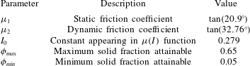
To specify the parameters appearing in the constitutive laws (2.9c
) and (2.10), we suppose that the flow is characterised by the rheological parameters
 $\unicode[STIX]{x1D707}_{1,2}$
and
 $I_{0}$
obtained by Forterre & Pouliquen (Reference Forterre and Pouliquen2003) for the inclined plane flow of glass beads (
 $d=0.5~\text{mm}$
), as summarised in table 1. The volume fraction in this case is typically found to be approximately constant over most of the flow, with this constant decreasing for increasing inclination
 $\unicode[STIX]{x1D703}$
, except near the free surface where it rapidly decreases towards zero (MiDi Reference Midi2004; Kumaran & Maheshwari Reference Kumaran and Maheshwari2012; Mandal & Khakhar Reference Mandal and Khakhar2016). For our purposes, based on the data of Ancey (Reference Ancey2001), we have taken
 $\unicode[STIX]{x1D719}_{max}=0.65$
and
 $\unicode[STIX]{x1D719}_{min}=0.05$
as reasonable estimates for these parameters. In reality, one could allow
 $\unicode[STIX]{x1D719}_{max}=\unicode[STIX]{x1D719}_{max}(\unicode[STIX]{x1D703})$
given that the bulk density is found to vary with inclination; however, we avoid such complications here. Our emphasis is on the role played by compressibility in the flow, and thus incorporating additional complexity by estimating (phenomenological) model parameters using experimental data is unwarranted.
Finally, it is reasonable to anticipate a hydrostatic scaling for pressure in this problem, and hence we follow Barker et al. (Reference Barker, Schaeffer, Shearer and Gray2017) by taking
 ${\mathcal{P}}=\unicode[STIX]{x1D70C}_{s}gd$
. Note, however, that the inclusion of the external acceleration
 $g$
in the constitutive relation (2.10) may invalidate the material frame-indifference of the model (Goddard & Lee Reference Goddard and Lee2018). This critique is pertinent given that frame-indifference is evidently a common assumption in continuum and solid mechanics (see Fowler Reference Fowler2011, p. 111); however, it conceivably may not apply for granular material (Higham Reference Higham2015, p. 666). In any case this consideration, which is more philosophical in nature, does not affect the stability analysis presented below, and may be avoided by utilising an alternative pressure scaling for
 ${\mathcal{P}}$
as opposed to the extrinsic hydrostatic scaling. This point is revisited in § 4.2.
Sketch of the chute flow geometry under consideration. Here
 $h_{0}$
and
 $u_{0}(z)$
refer to the base state flow depth and velocity, respectively.

Parameter values assumed for the inclined plane flow. Rheological parameters as determined by Jop et al. (Reference Jop, Forterre and Pouliquen2005) and
 $\unicode[STIX]{x1D719}_{max}$
and
 $\unicode[STIX]{x1D719}_{min}$
estimates taken from Ancey (Reference Ancey2001).

3.1 Base state and non-dimensionalisation
Appropriate non-dimensionalisation of our equations is motivated by examining the base state of the system, which is easily obtained by seeking a unidirectional steady flow
 $\boldsymbol{u}=(u_{0}(z),0)$
of constant depth
 $h=h_{0}$
and solid fraction
 $\unicode[STIX]{x1D719}=\unicode[STIX]{x1D719}_{0}(z)$
(Barker et al.
Reference Barker, Schaeffer, Shearer and Gray2017). As this flow is incompressible, we have
 $f=0$
, and hence it follows from conservation of momentum and (2.5) that
 $\unicode[STIX]{x03C4}=p\tan \unicode[STIX]{x1D703}=\unicode[STIX]{x1D707}(I)p$
. Thus
 $$\begin{eqnarray}\displaystyle I=I_{\unicode[STIX]{x1D703}}=\unicode[STIX]{x1D707}^{-1}(\tan \unicode[STIX]{x1D703}) & & \displaystyle\end{eqnarray}$$
is constant throughout the flow. To ensure that
 $I$
is positive and bounded, the inclination must exist in the range
 $\tan ^{-1}\unicode[STIX]{x1D707}_{1}<\unicode[STIX]{x1D703}<\tan ^{-1}\unicode[STIX]{x1D707}_{2}$
, i.e. the range for which steady uniform chute flow is obtained by Forterre & Pouliquen (Reference Forterre and Pouliquen2003). Negative and unbounded
 $I$
represent transitions to the quasi-static and gaseous regimes, respectively. From conservation of momentum and the definition of the inertial number, we have that the base state pressure and velocity profiles (assuming that
 $u$
increases with
 $z$
(Gray & Edwards Reference Gray and Edwards2014)) are determined by the ordinary differential equations
 $$\begin{eqnarray}\displaystyle \frac{\text{d}p_{0}}{\text{d}z}=-\unicode[STIX]{x1D70C}_{s}\unicode[STIX]{x1D719}_{0}g\cos \unicode[STIX]{x1D703},\quad p_{0}(h_{0})=0,\quad \frac{\text{d}u_{0}}{\text{d}z}=\frac{I_{\unicode[STIX]{x1D703}}}{d}\sqrt{\frac{p_{0}}{\unicode[STIX]{x1D70C}_{s}}},\quad u_{0}(0)=0, & & \displaystyle\end{eqnarray}$$
where from (2.8) and (2.10)
 $\unicode[STIX]{x1D719}_{0}$
is given by
 $$\begin{eqnarray}\displaystyle \unicode[STIX]{x1D719}_{0}=\unicode[STIX]{x1D719}_{min}+\frac{\unicode[STIX]{x0394}\unicode[STIX]{x1D719}\left(\displaystyle \frac{2p_{0}b}{\unicode[STIX]{x1D6FD}(I_{\unicode[STIX]{x1D703}})\unicode[STIX]{x1D70C}_{s}gd}\right)}{1+\displaystyle \frac{2p_{0}b}{\unicode[STIX]{x1D6FD}(I_{\unicode[STIX]{x1D703}})\unicode[STIX]{x1D70C}_{s}gd}},\quad \unicode[STIX]{x0394}\unicode[STIX]{x1D719}=\unicode[STIX]{x1D719}_{max}-\unicode[STIX]{x1D719}_{min}. & & \displaystyle\end{eqnarray}$$
Thus (3.4) suggests we non-dimensionalise the model using the natural scales
 $$\begin{eqnarray}\displaystyle & \displaystyle x,z,h\sim h_{0},\quad t\sim \frac{h_{0}}{U},\quad \boldsymbol{u}\sim U=\frac{I_{\unicode[STIX]{x1D703}}\sqrt{gh_{0}^{3}\cos \unicode[STIX]{x1D703}}}{d}, & \displaystyle\end{eqnarray}$$
 $$\begin{eqnarray}\displaystyle & \displaystyle p,\unicode[STIX]{x03C4}_{ij},Y\sim \unicode[STIX]{x1D70C}_{s}gh_{0}\cos \unicode[STIX]{x1D703},\quad \unicode[STIX]{x1D60B}_{ij}\sim \frac{U}{h_{0}}. & \displaystyle\end{eqnarray}$$
 $$\begin{eqnarray}\displaystyle \frac{\text{d}p_{0}}{\text{d}z}=-\unicode[STIX]{x1D719}_{0},\quad p_{0}(1)=0,\quad \frac{\text{d}u_{0}}{\text{d}z}=\sqrt{p_{0}},\quad u_{0}(0)=0, & & \displaystyle\end{eqnarray}$$
while
 $\unicode[STIX]{x1D719}_{0}$
is given by
 $$\begin{eqnarray}\displaystyle \unicode[STIX]{x1D719}_{0}=\unicode[STIX]{x1D719}_{min}+\frac{\unicode[STIX]{x0394}\unicode[STIX]{x1D719}(2p_{0}\unicode[STIX]{x1D712})}{1+2p_{0}\unicode[STIX]{x1D712}},\quad \unicode[STIX]{x1D712}=\frac{bh_{0}\cos \unicode[STIX]{x1D703}}{\unicode[STIX]{x1D6FD}(I_{\unicode[STIX]{x1D703}})d}, & & \displaystyle\end{eqnarray}$$
and
 $\unicode[STIX]{x1D712}$
is a non-dimensional parameter. Note that one recovers a uniform volume fraction profile, as predicted from the incompressible rheology, in the limit
 $\unicode[STIX]{x0394}\unicode[STIX]{x1D719}\rightarrow 0$
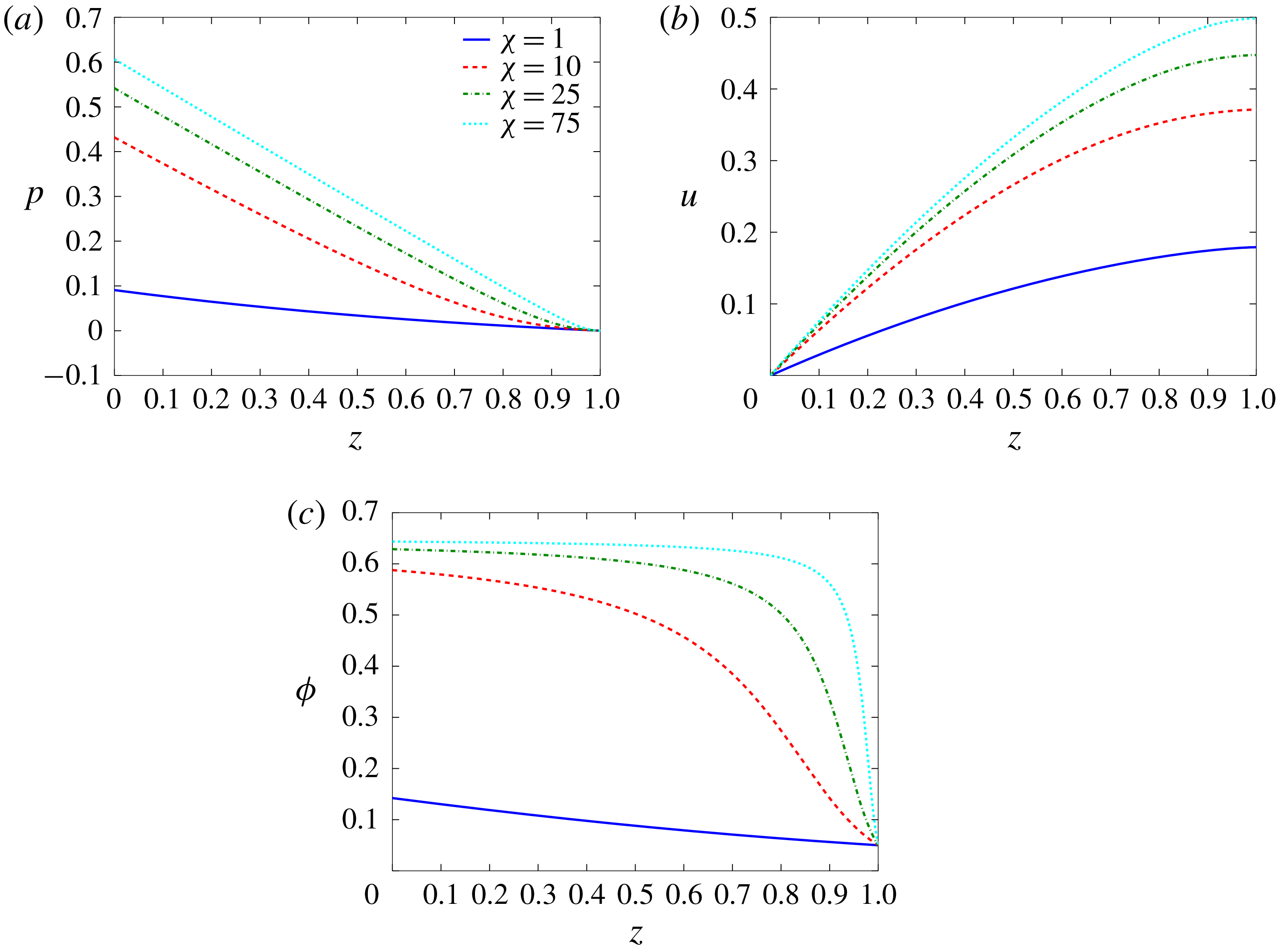
. The ordinary differential equation system (3.7) can readily be solved numerically (using ode45 in Matlab) to give the base state profiles illustrated in figure 2 for various values of
 $\unicode[STIX]{x1D712}$
. We recover an approximately lithostatic pressure distribution (figure 2
a), while figure 2(b) demonstrates the Bagnold velocity profile for granular chute flow (MiDi Reference Midi2004).

As discussed by Barker et al. (Reference Barker, Schaeffer, Shearer and Gray2017), the parameter
 $\unicode[STIX]{x1D712}$
essentially controls the variation in the base state solid fraction profile over a given
 $\unicode[STIX]{x0394}\unicode[STIX]{x1D719}$
range, and hence its mean value (figure 2
c). Experimental evidence illustrates that for steady uniform flow the solid fraction is approximately constant over the interior of the flow before rapidly decreasing near the free surface (see § 3), and thus this suggests the use of a large value for
 $\unicode[STIX]{x1D712}$
. While this parameter depends both on the ratio of the base state flow thickness to particle size
 $h_{0}/d$
(
 ${\sim}10$
) and inclination
 $\unicode[STIX]{x1D703}$
from (3.8), it is also proportional to the largely unconstrained parameter
 $b$
. In practice, it may be possible to determine this free parameter using suitable base state flow data (e.g. see § 4.2). In the case of inclined plane flow, provided knowledge of
 $h_{0}$
,
 $\unicode[STIX]{x1D703}$
and
 $d$
, one could fit the base state volume fraction profile (3.8) to available experimental data in order to yield an estimate for
 $b$
. However, in practice we anticipate that, in a similar manner to the parameters characterising the
 $\unicode[STIX]{x1D707}(I)$
phenomenological law (2.9c
), this parameter varies with the material properties of the granular medium and bed roughness conditions.
In the absence of additional information, we assume
 $\unicode[STIX]{x1D712}$
is a relatively large free parameter (e.g.
 $25\leqslant \unicode[STIX]{x1D712}\leqslant 100$
). Note that at various points throughout this work, results are illustrated for the representative value
 $\unicode[STIX]{x1D712}=75$
given that, in this case, (i) the base state
 $\unicode[STIX]{x1D719}$
profile mimics that found experimentally and (ii) we find
 $\overline{\unicode[STIX]{x1D719}_{0}}\approx 0.606$
, in agreement with the average solid fraction of
 $0.59\pm 0.03$
for steady chute flows as obtained by Pouliquen (Reference Pouliquen1999). Note that taking
 $\unicode[STIX]{x1D712}\rightarrow \infty$
introduces a discontinuity in the base state solid fraction profile given that
 $\unicode[STIX]{x1D719}_{0}$
must reduce to
 $\unicode[STIX]{x1D719}_{min}$
at the free surface (from (3.8)). This boundary layer will naturally introduce numerical difficulties when discretising
 $\unicode[STIX]{x1D719}_{0}$
(and derivatives thereof) in the solution of the generalised eigenvalue problem outlined in § 3.3. Thus we avoid taking
 $\unicode[STIX]{x1D712}$
too large (
 ${>}100$
say) to circumvent such issues.
Finally, using the scaling (3.6), the non-dimensional CIDR system is given by
 $$\begin{eqnarray}\displaystyle & \displaystyle \frac{\unicode[STIX]{x2202}\unicode[STIX]{x1D719}}{\unicode[STIX]{x2202}t}+\unicode[STIX]{x1D735}\boldsymbol{\cdot }(\unicode[STIX]{x1D719}\boldsymbol{u})=0, & \displaystyle\end{eqnarray}$$
 $$\begin{eqnarray}\displaystyle & \displaystyle F^{2}\unicode[STIX]{x1D719}\left(\frac{\unicode[STIX]{x2202}\boldsymbol{u}}{\unicode[STIX]{x2202}t}+(\boldsymbol{u}\boldsymbol{\cdot }\unicode[STIX]{x1D735})\boldsymbol{u}\right)=-\unicode[STIX]{x1D735}p+\unicode[STIX]{x1D735}\boldsymbol{\cdot }\left(\unicode[STIX]{x03C4}\frac{\unicode[STIX]{x1D63F}}{\Vert \unicode[STIX]{x1D63F}\Vert }\right)+\unicode[STIX]{x1D719}(\unicode[STIX]{x1D707}_{\unicode[STIX]{x1D703}},-1), & \displaystyle\end{eqnarray}$$
 $$\begin{eqnarray}\displaystyle \unicode[STIX]{x1D735}\boldsymbol{\cdot }\boldsymbol{u}=2f(p,\unicode[STIX]{x1D719},I)\Vert \unicode[STIX]{x1D63F}\Vert ,\quad \unicode[STIX]{x03C4}=Y(p,\unicode[STIX]{x1D719},I), & & \displaystyle\end{eqnarray}$$
where
 $$\begin{eqnarray}\displaystyle Y=\unicode[STIX]{x1D6FC}(I)p-\frac{\unicode[STIX]{x1D6FD}(I_{\unicode[STIX]{x1D703}})\unicode[STIX]{x1D712}p^{2}}{{\hat{C}}(\unicode[STIX]{x1D713})},\quad f=\unicode[STIX]{x1D6FD}(I)-\frac{2\unicode[STIX]{x1D6FD}(I_{\unicode[STIX]{x1D703}})\unicode[STIX]{x1D712}p}{{\hat{C}}(\unicode[STIX]{x1D713})},\quad I=\frac{2I_{\unicode[STIX]{x1D703}}\Vert \unicode[STIX]{x1D63F}\Vert }{\sqrt{p}}, & & \displaystyle\end{eqnarray}$$
with
 $I_{\unicode[STIX]{x1D703}}$
given by (3.3). Here we have defined the Froude number
 $F$
and constant
 $\unicode[STIX]{x1D707}_{\unicode[STIX]{x1D703}}$
as
 $$\begin{eqnarray}\displaystyle F=\frac{U}{\sqrt{gh_{0}\cos \unicode[STIX]{x1D703}}},\quad \unicode[STIX]{x1D707}_{\unicode[STIX]{x1D703}}=\tan \unicode[STIX]{x1D703}. & & \displaystyle\end{eqnarray}$$
In addition, the surface boundary conditions (3.1) and (3.2) become
 $$\begin{eqnarray}\displaystyle \left.\begin{array}{@{}l@{}}\displaystyle ph_{x}-\unicode[STIX]{x03C4}_{11}h_{x}+\unicode[STIX]{x03C4}_{12}=0,\quad -\unicode[STIX]{x03C4}_{12}h_{x}-p+\unicode[STIX]{x03C4}_{22}=0,\\ \displaystyle v=h_{t}+uh_{x},\end{array}\right\}\quad \text{at}~z=h(x,t), & & \displaystyle\end{eqnarray}$$
respectively, supplemented with the no-slip condition
 $\boldsymbol{u}=0$
at
 $z=0$
.
3.2 Linear stability analysis
The linear stability of the base state outlined in § 3.1 is analysed using a standard normal mode analysis (e.g. Drazin & Reid Reference Drazin and Reid1981, chap. 4). We consider perturbations of the form
 $$\begin{eqnarray}\displaystyle [u,v,\unicode[STIX]{x1D719},p,h]=[u_{0}(z),0,\unicode[STIX]{x1D719}_{0}(z),p_{0}(z),1]+[\tilde{u} ,\tilde{v},\tilde{\unicode[STIX]{x1D719}},\tilde{p},\tilde{h}](x,z,t), & & \displaystyle\end{eqnarray}$$
where perturbations are represented by the tilde variables. We then substitute these expansions into the governing equations (3.9), (3.10) and (3.13) and linearise the resulting system. After some tedious but nonetheless relatively straightforward algebra, we obtain
 $$\begin{eqnarray}\displaystyle & \displaystyle \tilde{\unicode[STIX]{x1D719}}_{t}+u_{0}\tilde{\unicode[STIX]{x1D719}}_{x}+\unicode[STIX]{x1D719}_{0}\tilde{u} _{x}+(\unicode[STIX]{x1D719}_{0}\tilde{v})_{z}=0, & \displaystyle\end{eqnarray}$$
 $$\begin{eqnarray}\displaystyle & \displaystyle F^{2}\unicode[STIX]{x1D719}_{0}(\tilde{u} _{t}+u_{0}\tilde{u} _{x}+u_{0}^{\prime }\tilde{v})=-\tilde{p}_{x}+\unicode[STIX]{x1D702}_{0}(2\tilde{u} _{x}/3-\tilde{v}_{z}/3)_{x}+[A_{p}\tilde{p}+A_{\unicode[STIX]{x1D719}}\tilde{\unicode[STIX]{x1D719}}+A_{u}(\tilde{u} _{z}+\tilde{v}_{x})]_{z}+\tilde{\unicode[STIX]{x1D719}}\unicode[STIX]{x1D707}_{\unicode[STIX]{x1D703}}, & \displaystyle \nonumber\\ \displaystyle & & \displaystyle\end{eqnarray}$$
 $$\begin{eqnarray}\displaystyle & \displaystyle F^{2}\unicode[STIX]{x1D719}_{0}(\tilde{v}_{t}+u_{0}\tilde{v}_{x})=-\tilde{p}_{z}+(\unicode[STIX]{x1D702}_{0}[2\tilde{v}_{z}/3-\tilde{u} _{x}/3])_{z}+A_{p}\tilde{p}_{x}+A_{\unicode[STIX]{x1D719}}\tilde{\unicode[STIX]{x1D719}}_{x}+A_{u}(\tilde{u} _{z}+\tilde{v}_{x})_{x}-\tilde{\unicode[STIX]{x1D719}}, & \displaystyle \nonumber\\ \displaystyle & & \displaystyle\end{eqnarray}$$
 $$\begin{eqnarray}\displaystyle & \displaystyle \tilde{u} _{x}+\tilde{v}_{z}=C_{p}\tilde{p}+C_{\unicode[STIX]{x1D719}}\tilde{\unicode[STIX]{x1D719}}+C_{u}(\tilde{u} _{z}+\tilde{v}_{x}). & \displaystyle\end{eqnarray}$$
 $z$
, where
 $u_{0}^{\prime }$
is non-constant, and subscripts
 $(~)_{x,z,t}$
denote partial differentiation. This system is supplemented with the boundary conditions
 $$\begin{eqnarray}\displaystyle & \displaystyle \tilde{u} =\tilde{v}=0\quad \text{at}~z=0, & \displaystyle\end{eqnarray}$$
 $$\begin{eqnarray}\displaystyle & \displaystyle \left.\begin{array}{@{}l@{}}\displaystyle \unicode[STIX]{x1D707}_{\unicode[STIX]{x1D703}}p_{0}^{\prime }\tilde{h}+A_{p}\tilde{p}+A_{\unicode[STIX]{x1D719}}\tilde{\unicode[STIX]{x1D719}}+A_{u}(\tilde{u} _{z}+\tilde{v}_{x})=0,\\ \displaystyle -p_{0}^{\prime }\tilde{h}-\tilde{p}+\unicode[STIX]{x1D702}_{0}(2\tilde{v}_{z}/3-\tilde{u} _{x}/3)=0,\\ \displaystyle \tilde{v}=\tilde{h}_{t}+u_{0}\tilde{h}_{x},\end{array}\right\}\quad \text{at}~z=1. & \displaystyle\end{eqnarray}$$
 $A$
,
 $C$
and
 $\unicode[STIX]{x1D702}_{0}$
are defined in appendix A. These coefficients are non-constant in general given that the base state velocity, pressure and solid fraction profiles are all
 $z$
-dependent. In contrast to the analysis carried out by Barker et al. (Reference Barker, Schaeffer, Bohorquez and Gray2015), the linearised system (3.15) includes convective inertial effects such as wavevector stretching (Goddard & Lee Reference Goddard and Lee2017). Note that
 $\tilde{h}$
can be eliminated from the problem entirely via the surface boundary condition (3.16b
). Some care is required when handling the surface boundary conditions (3.16b
) since both
 $A_{u}$
and
 $\unicode[STIX]{x1D702}_{0}$
vanish at the free surface, i.e. the boundary conditions are degenerate unless
 $\tilde{u} _{z}$
and
 $\tilde{v}_{z}$
are singular. To allow for the possibility that the combinations
 $A_{u}\tilde{u} _{z}$
and
 $\unicode[STIX]{x1D702}_{0}\tilde{v}_{z}$
are non-zero there, we follow the approach of Forterre (Reference Forterre2006) and introduce auxiliary variables
 $\widetilde{\unicode[STIX]{x1D6E4}}$
and
 $\widetilde{\unicode[STIX]{x1D6F9}}$
defined as
 $$\begin{eqnarray}\displaystyle \widetilde{\unicode[STIX]{x1D6E4}}=A_{u}(\tilde{u} _{z}+\tilde{v}_{x}),\quad \widetilde{\unicode[STIX]{x1D6F9}}=\unicode[STIX]{x1D702}_{0}\left(\frac{2\tilde{v}_{z}}{3}-\frac{\tilde{u} _{x}}{3}\right), & & \displaystyle\end{eqnarray}$$
so that the boundary conditions are now regular in these variables. One should note, however, that (3.16b
) differs from the equivalent linearised boundary condition in the IIDR model (see Forterre Reference Forterre2006, (2.12)) due to the presence of the additional
 $\widetilde{\unicode[STIX]{x1D6F9}}$
stress term. Incompressibility implies that this stress term should vanish at the free surface; however, by consideration of the linearised flow rule (3.15d
), it appears there is no reason a priori to assume
 $\widetilde{\unicode[STIX]{x1D6F9}}=0$
in the compressible model. As such, we have chosen to include this term in the boundary conditions.
Note that (3.15) is a variable-coefficient linear system whose coefficients are independent of both time and the downstream direction. Therefore, following standard practice in the literature (see e.g. Drazin & Reid (Reference Drazin and Reid1981, chap. 4) and Chandrasekhar (Reference Chandrasekhar1981, chap. 1)), we seek normal mode solution
 $$\begin{eqnarray}\displaystyle [\tilde{u} ,\tilde{v},\tilde{\unicode[STIX]{x1D719}},\tilde{p}]=\text{e}^{\text{i}kx+\unicode[STIX]{x1D70E}t}[\hat{u} ,\hat{v},\hat{\unicode[STIX]{x1D719}},\hat{p}](z), & & \displaystyle\end{eqnarray}$$
where
 $\hat{u} =\hat{u} (z)$
, and similarly so for the other eigenfunctions (Malik Reference Malik1990; Alam & Nott Reference Alam and Nott1998; Forterre Reference Forterre2006). While a perturbation solution in terms of Kelvin modes may be suitable in the case of unbounded flow (Alam & Nott Reference Alam and Nott1997; Goddard & Lee Reference Goddard and Lee2017), the imposition of vertical boundary conditions in our case restricts the perturbation solution to the form (3.18) (Wang, Jackson & Sundaresan Reference Wang, Jackson and Sundaresan1996). Here
 $k\in \mathbb{R}$
is the downstream wavenumber and
 $c=\unicode[STIX]{x1D70E}/k$
, where
 $\unicode[STIX]{x1D70E}\in \mathbb{C}$
, is the wave speed. Thus for a given wavenumber the linear evolution of the system is governed by the growth rate
 $\text{Re}(\unicode[STIX]{x1D70E})$
and angular frequency
 $-\text{Im}(\unicode[STIX]{x1D70E})$
. This is referred to as a temporal stability analysis, which contrasts with a spatial stability analysis in which a pulsation
 $\unicode[STIX]{x1D70E}=-\text{i}\unicode[STIX]{x1D714}$
for
 $\unicode[STIX]{x1D714}\in \mathbb{R}$
is specified and
 $k\in \mathbb{C}$
is the eigenvalue of interest (see Schmid & Henningson Reference Schmid and Henningson2001, chap. 7). A spatial stability analysis is carried out in Forterre (Reference Forterre2006) and Gray & Edwards (Reference Gray and Edwards2014) in order to compare their results directly with the spatial stability data of Forterre & Pouliquen (Reference Forterre and Pouliquen2003); however, we avoid this approach given that the eigenvalue
 $k$
appears quadratically in the stability problem, which is typically more difficult to handle numerically (Malik Reference Malik1990; Varsakelis & Papalexandris Reference Varsakelis and Papalexandris2016). In any case, we discuss in § 3.4 how the temporal analysis can be used to compare against the spatial stability data.
Substitution of (3.18) into the linearised equations yields a system of four linear differential–algebraic equations (see (A 3) and (A 4) in appendix A) for the velocity, pressure and solid fraction perturbations, forming a generalised eigenvalue problem in
 $\unicode[STIX]{x1D70E}$
. Note that in the incompressible
 $\unicode[STIX]{x1D707}(I)$
limit, i.e. by taking
 $f=0$
,
 $\unicode[STIX]{x1D719}_{0}=\text{const.}$
,
 $\tilde{\unicode[STIX]{x1D719}}=0$
and
 $Y=\unicode[STIX]{x1D707}(I)p$
, equations (3.15) and (3.16) reduce to the system presented in Forterre (Reference Forterre2006), as expected.
3.3 Numerical method for stability problem
Following standard practice in the hydrodynamic stability of compressible flows (e.g. Malik Reference Malik1990; Malik, Alam & Dey Reference Malik, Alam and Dey2006), we implement a Chebyshev collocation method (see Trefethen Reference Trefethen2000; Boyd Reference Boyd2001, chap. 6) to solve the stability problem (A 3) subject to the boundary conditions (A 4). We propose a series expansion of a given eigenfunction
 $Q(z)$
in terms of the Chebyshev polynomials
 $T_{n}(\unicode[STIX]{x1D709})=\cos (n\cos ^{-1}\unicode[STIX]{x1D709})$
, i.e.
 $$\begin{eqnarray}\displaystyle Q(z)=\mathop{\sum }_{n=0}^{N}a_{n}^{Q}T_{n}(\unicode[STIX]{x1D709}), & & \displaystyle\end{eqnarray}$$
where
 $N$
is the degree of the expansion,
 $a_{n}^{Q}$
are the expansion coefficients for eigenfunction
 $Q$
and we define the change of variables
 $\unicode[STIX]{x1D709}=2z-1$
to map the physical domain
 $z\in [0,1]$
to the Chebyshev domain
 $\unicode[STIX]{x1D709}\in [-1,1]$
. The governing equations are then collocated at the Gauss–Lobatto points
 $$\begin{eqnarray}\displaystyle \unicode[STIX]{x1D709}_{i}^{{\mathcal{G}}{\mathcal{L}}}=\cos \left(\frac{\unicode[STIX]{x03C0}i}{N}\right),\quad i=0,\ldots ,N, & & \displaystyle\end{eqnarray}$$
i.e. the extrema of the polynomial
 $T_{n}$
, while evaluation at the boundary nodes is replaced by the relevant boundary conditions.
However, discretisation of the stability problem in this manner requires the use of artificial boundary conditions for the solid fraction perturbation. It is well known that the numerical solution of generalised eigenvalue problems with artificial boundary conditions can suffer from spurious (i.e. unphysical) eigenvalues (e.g. see Alam & Nott (Reference Alam and Nott1998) and Boyd (Reference Boyd2001, chap. 7)). To avoid the specification of such boundary conditions, we follow the approach of Müller & Kleiser (Reference Müller and Kleiser2008) by implementing a staggered collocation method. In particular, the momentum equations are evaluated on the Gauss–Lobatto points
 $\unicode[STIX]{x1D709}_{i}^{{\mathcal{G}}{\mathcal{L}}}$
, while conservation of mass, the flow rule and the definitions of the auxiliary variables (3.17) are collocated on the Gauss points
 $$\begin{eqnarray}\displaystyle \unicode[STIX]{x1D709}_{i}^{{\mathcal{G}}}=\cos \left[\frac{(2i+1)\unicode[STIX]{x03C0}}{2N}\right],\quad i=0,\ldots ,N-1. & & \displaystyle\end{eqnarray}$$
Thus the velocity eigenfunctions
 $(\hat{u} ,\hat{v})$
are expanded as
 $N+1$
term series, while the other eigenfunctions
 $(\hat{\unicode[STIX]{x1D719}},\hat{p},\hat{\unicode[STIX]{x1D6E4}},\hat{\unicode[STIX]{x1D6F9}})$
are of one degree less. Evaluation of the Chebyshev polynomials (and derivatives thereof) at the Gauss–Lobatto and Gauss points is carried out using the formulae detailed in appendix A.2 of Boyd (Reference Boyd2001).
Upon discretisation of the stability problem in this manner, we obtain the system
 $$\begin{eqnarray}\displaystyle \unicode[STIX]{x1D63C}\boldsymbol{Q}=\unicode[STIX]{x1D63D}\unicode[STIX]{x1D70E}\boldsymbol{Q}, & & \displaystyle\end{eqnarray}$$
where
 $\unicode[STIX]{x1D63C}$
is a
 $(6N+2)^{2}$
dense matrix,
 $\boldsymbol{Q}$
is the vector of unknown coefficients and
 $\unicode[STIX]{x1D63D}$
is a rank-deficient matrix, which results in the system (3.22) possessing a large number of infinite eigenvalues. Thus, we adopt the approach of Moyles & Wetton (Reference Moyles and Wetton2015) and consider instead
 $$\begin{eqnarray}\displaystyle \unicode[STIX]{x1D63D}\boldsymbol{Q}=\frac{1}{\unicode[STIX]{x1D70E}}\unicode[STIX]{x1D63C}\boldsymbol{Q}=\unicode[STIX]{x1D63C}\unicode[STIX]{x1D706}\boldsymbol{Q},\quad \unicode[STIX]{x1D706}=\frac{1}{\unicode[STIX]{x1D70E}}\;\Longrightarrow \;\unicode[STIX]{x1D70E}=\frac{\bar{\unicode[STIX]{x1D706}}}{|\unicode[STIX]{x1D706}|^{2}}, & & \displaystyle\end{eqnarray}$$
which is both more computationally efficient and accurate to solve. The eigenvalues
 $\unicode[STIX]{x1D706}$
and eigenvectors
 $\boldsymbol{Q}$
can then be obtained using the standard eig solver in Matlab. For linear stability we are only interested in the value of
 $\unicode[STIX]{x1D70E}$
with maximal real part, and henceforth we assume that
 $\unicode[STIX]{x1D70E}$
represents this maximal value.
3.4 Incompressible limit
Our stability analysis of the CIDR model represents a generalisation of the IIDR analysis presented in Forterre (Reference Forterre2006), and thus it is natural to consider an incompressible limit of our eigenvalue problem as a means of validation of the numerical method. Given that variability in the solid fraction is characterised by the quantity
 $\unicode[STIX]{x0394}\unicode[STIX]{x1D719}=\unicode[STIX]{x1D719}_{max}-\unicode[STIX]{x1D719}_{min}$
, we can consider an incompressible limit by taking
 $\unicode[STIX]{x0394}\unicode[STIX]{x1D719}\rightarrow 0$
. Indeed, Barker et al. (Reference Barker, Schaeffer, Shearer and Gray2017) demonstrate that the CIDR model suitably reduces to its incompressible equivalent in this limit. To make a sensible comparison between our results and those of Forterre (Reference Forterre2006), we must take into account a number of important differences between the two studies. The first simply relates to the choice of scales and the subsequent definition of the Froude number
 $F$
, which in this work is given by (3.12), i.e.
 $F=I_{\unicode[STIX]{x1D703}}h_{0}/d$
. However since the solid fraction is assumed constant in Forterre (Reference Forterre2006), which we denote
 $\unicode[STIX]{x1D719}_{Bulk}$
, the authors incorporate it into their scaling of the model. As such, we find that their Froude number,
 ${\mathcal{F}}$
, relates to ours via
 $$\begin{eqnarray}\displaystyle {\mathcal{F}}=\frac{2\sqrt{\unicode[STIX]{x1D719}_{Bulk}}}{5}F, & & \displaystyle\end{eqnarray}$$
where, for simplicity, we assume that
 $\unicode[STIX]{x1D719}_{Bulk}$
is given by the mean value of our base state solid fraction profile, i.e.
 $\unicode[STIX]{x1D719}_{Bulk}=\overline{\unicode[STIX]{x1D719}_{0}}$
.
The second key difference relates to the spatial stability analysis in which perturbations to the base state are proportional to
 $\text{e}^{\text{i}k^{\ast }x-\text{i}\unicode[STIX]{x1D714}^{\ast }t}$
, where
 $k^{\ast }\in \mathbb{C}$
,
 $\unicode[STIX]{x1D714}^{\ast }\in \mathbb{R}$
and asterisked quantities refer to those used by Forterre (Reference Forterre2006). Thus the growth rate and wave speed are given by
 $\unicode[STIX]{x1D70E}^{\ast }=-\text{Im}(k^{\ast })$
and
 $c^{\ast }=\unicode[STIX]{x1D714}^{\ast }/\text{Re}(k^{\ast })$
, respectively. In order to compare our results against the spatial dispersion relations, we perform an equivalent analysis by seeding the eigenvalue solver with imaginary values for the wavenumber and searching over complex
 $k$
space. The set of eigenvalues which have real part zero can thus be interpreted as values for the perturbation frequency
 $\unicode[STIX]{x1D714}=-\text{Im}(\unicode[STIX]{x1D70E})$
. Hence from this set we can obtain values for the growth rate
 $-\text{Im}(k)$
and wave speed
 $\unicode[STIX]{x1D714}/\text{Re}(k)$
, allowing for direct comparison with the results of Forterre (Reference Forterre2006).
Spatial dispersion relations for the dimensionless (a) growth rate and (b) wave speed as a function of the perturbation frequency. The solid line indicates the predicted profile from the solution of the full compressible problem with
 $\unicode[STIX]{x0394}\unicode[STIX]{x1D719}=10^{-3}$
, while the markers represent the equivalent prediction from the IIDR model of Forterre (Reference Forterre2006). Parameter values as in table 1 with
 $\unicode[STIX]{x1D719}_{min}=0.649$
,
 $N=100$
,
 $\unicode[STIX]{x1D703}=29^{\circ }$
,
 ${\mathcal{F}}=1.02$
and
 $\unicode[STIX]{x1D712}=75$
.

Such a comparison is illustrated in figure 3 where the leading growth rate and corresponding wave speed are plotted as a function of the frequency
 $\unicode[STIX]{x1D714}$
. Note that the time scales in each study differ by a factor of
 $5/(2\sqrt{\unicode[STIX]{x1D719}_{Bulk}})$
, and hence to make a practical comparison between the two, we rescale our computed eigenvalue (and thus
 $\unicode[STIX]{x1D714}$
) by this factor. For
 $\unicode[STIX]{x0394}\unicode[STIX]{x1D719}=10^{-3}$
we observe excellent agreement between the spatial dispersion relation computed using our numerical method and that given by Forterre (Reference Forterre2006) (see figure 2 therein), with a slight discrepancy between the two at larger values of
 $\unicode[STIX]{x1D714}$
(corresponding to larger
 $\text{Re}(k)$
). Such differences at large
 $k$
are anticipated given that the incompressible rheology is linearly ill-posed. The overall agreement in figure 3 provides strong evidence for the veracity of the solver. Further validation by comparison with a long-wavelength asymptotic analysis of the stability problem is presented in the supplementary material available at https://doi.org/10.1017/jfm.2019.43.
3.5 Results
Given the validation of the numerical method outlined in § 3.4, we can now compare the stability predictions of the compressible model with the experimental results of Forterre & Pouliquen (Reference Forterre and Pouliquen2003), upon which the rheological parameters assumed in table 1 have been calibrated. As such, assuming fixed values for
 $\unicode[STIX]{x1D719}_{max}$
and
 $\unicode[STIX]{x1D719}_{min}$
,
 $\unicode[STIX]{x1D712}$
represents the only variable parameter in this analysis. This comparison is carried out in § 3.5.2, while predictions pertaining to the temporal stability of the system are presented below.
3.5.1 Temporal stability
Contour plot of the dimensionless leading growth rate in
 $(k,F)$
space for
 $\unicode[STIX]{x1D712}=75$
,
 $\unicode[STIX]{x1D703}=29^{\circ }$
,
 $N=100$
and parameter values in table 1. The red line traces the maximal growth rate as a function of
 $k$
for fixed
 $F$
. The colour scale has been truncated at
 $-10^{-3}$
for enhancement, while the numerical data have been interpolated onto a finer mesh (
 $10^{-3}\times 10^{-2}$
) using a cubic spline interpolation.

Assuming
 $\unicode[STIX]{x1D70E}\in \mathbb{C}$
and
 $k\in \mathbb{R}$
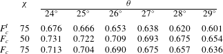
, an indicative contour plot of the dimensionless growth rate as a function of the downstream wavenumber and Froude number is illustrated in figure 4. Here the eigenvalue and Froude number have been rescaled as in § 3.4 to allow for direct comparison with Forterre (Reference Forterre2006). This dispersion relation allows us to approximate the critical Froude number
 $F_{c}$
above which the flow is unstable, i.e. the minimum
 $F$
such that
 $\text{Re}(\unicode[STIX]{x1D70E})>0$
for some
 $k$
. Typical values are indicated in table 2 for various
 $\unicode[STIX]{x1D712}$
. Note that in the incompressible limit
 $\unicode[STIX]{x0394}\unicode[STIX]{x1D719}=10^{-3}$
we obtain values for the critical Froude number
 $F_{c}^{I}$
as predicted by equation (2.13) of Forterre (Reference Forterre2006). The compressible model is found to admit slightly larger values for
 $F_{c}$
than the IIDR model; however, the difference between the two decreases for increasing
 $\unicode[STIX]{x1D712}$
, as expected.
(a) Maximal growth rate and (b) its corresponding wavenumber as a function of
 $F$
for parameter values as in figure 4.

Critical Froude number
 $F_{c}$
obtained for various
 $\unicode[STIX]{x1D703}$
and
 $\unicode[STIX]{x1D712}$
using
 $N=100$
and parameters as in table 1. Here,
 $F_{c}^{I}$
indicates the incompressible values obtained for
 $\unicode[STIX]{x0394}\unicode[STIX]{x1D719}=10^{-3}$
.

By tracing the maximal growth rate in
 $(k,F)$
space, we observe that this growth rate (figure 5
a) is a unimodal function of
 $F$
, with a sharp increase close to criticality and a slow decay thereafter, while the preferential wavenumber for growth (figure 5
b) continues to increase at large
 $F$
for the range considered. Both quantities demonstrate relatively weak dependence on the inclination
 $\unicode[STIX]{x1D703}$
. To our knowledge, no quantitative measurements of the temporal stability properties of granular chute flows are available for comparison with these predictions, while we are unable to make dimensional conversions given that the relevant length (
 $h_{0}$
) and time (
 $h_{0}/U$
) scales are problem-specific.
An estimate for typical roll wave spacing may be obtained by utilising the flow data provided in figure 16 of Forterre & Pouliquen (Reference Forterre and Pouliquen2003). For
 $F=1.02$
,
 $\unicode[STIX]{x1D703}=29^{\circ }$
,
 $h_{0}=5.3~\text{mm}$
and
 $U=21.7~\text{cm}~\text{s}^{-1}$
, we find a preferential wavelength of
 $\unicode[STIX]{x1D706}\approx 13~\text{cm}$
with an associated growth rate of
 ${\approx}0.5~\text{s}^{-1}$
. Although direct comparison cannot be made due to different rheological parameters and inclinations, we note that these estimates are of the same order as those predicted by Barker et al. (Reference Barker, Schaeffer, Shearer and Gray2017) using a depth-averaged regularised
 $\unicode[STIX]{x1D707}(I)$
rheology (see figure 13 therein). Moreover, we also note that this preferential wavelength is similar to the
 ${\sim}20~\text{cm}$
average observed in the bi-disperse granular roll wave experiments of Viroulet et al. (Reference Viroulet, Baker, Rocha, Johnson, Kokelaar and Gray2018). A quantitative comparison of the temporal stability predictions to experimental data would form an additional test of the CIDR model. However, the feasibility of performing such experiments remains an open question given that the natural temporal instability for glass beads was not observed in the chute flow experiments of Forterre & Pouliquen (Reference Forterre and Pouliquen2003), owing to the inclined plane being too short to observe the slow growth of the perturbations.
3.5.2 Spatial stability
Using the methodology outlined in § 3.4, we can also obtain results pertaining to the spatial stability of the system. We illustrate a representative dispersion relation in figure 6 for the spatial growth rate
 $\unicode[STIX]{x1D70E}$
and corresponding wave speed
 $c$
as a function of the perturbation frequency
 $\unicode[STIX]{x1D714}$
. We find that the predictions of the CIDR model are able to quantitatively match the experimental data in both cases, and indeed tend to perform better than the IIDR model predictions. To investigate the role played by compressibility when comparing to the dataset, the dispersion relations are obtained for various values of
 $\unicode[STIX]{x1D712}$
. Considering the dimensionless growth rate in figure 6(a), we can observe that its dominant effect is to shift the critical frequency
 $\unicode[STIX]{x1D714}_{c}$
to a lower value, particularly evident for the
 $\unicode[STIX]{x1D712}=25$
case in which the cutoff frequency is significantly underestimated. However larger values of
 $\unicode[STIX]{x1D712}$
, which are more representative of the base state solid fraction profile observed in experiments (see § 3.1), illustrate better agreement with the data. In particular the dispersion relations in this case, which are more or less identical to the IIDR model for
 $\unicode[STIX]{x1D714}<\unicode[STIX]{x1D714}_{c}$
, more accurately capture the experimental data at larger frequencies.
Theoretical (lines) and experimental (dots) spatial dispersion relations for the dimensionless (a) growth rate and (b) wave speed. Experimental data obtained from Forterre & Pouliquen (Reference Forterre and Pouliquen2003). Parameter values as in table 1 with
 $\unicode[STIX]{x1D703}=29^{\circ }$
,
 ${\mathcal{F}}=1.02$
and
 $N=100$
.

Dimensionless cutoff frequency as a function of the Froude number above criticality for (a) the incompressible case
 $\unicode[STIX]{x0394}\unicode[STIX]{x1D719}=10^{-3}$
and
 $\unicode[STIX]{x1D712}=75$
, and the compressible cases
 $\unicode[STIX]{x0394}\unicode[STIX]{x1D719}=0.6$
with (b)
 $\unicode[STIX]{x1D712}=50$
and (c)
 $\unicode[STIX]{x1D712}=75$
. The differences between the experimental data and model results are illustrated in (d) for: —— (a); - - - - (b); and – ⋅ – ⋅ (c). Datapoints have been categorised according to inclination, with Froude number increasing from left to right in each set. Computations have been carried out using parameter values as in table 1 and
 $N=100$
. The critical Froude numbers for the incompressible (
 $F_{c}^{I}$
) and compressible (
 $F_{c}$
) cases are given in table 2.

Similar behaviour is also observed for the wave speed in figure 6(b), where the compressibility acts to shift the spectrum towards lower values of
 $c$
, with larger
 $\unicode[STIX]{x1D712}$
again providing a good fit to the experimental data. These shifts in the dispersion relations are consistent with the depth-averaged IIDR model results of Gray & Edwards (Reference Gray and Edwards2014). It is interesting to note in figure 6 that neither the compressible nor incompressible models are able to capture the experimental growth rate maximum at
 $\unicode[STIX]{x1D714}\approx 0.4$
within experimental error, which is also the case for the depth-averaged IIDR model (Gray & Edwards Reference Gray and Edwards2014). Given that this maximum occurs at relatively small
 $\unicode[STIX]{x1D714}$
, elucidation of this issue may arise from performing an asymptotic analysis of the spatial stability problem; however, investigation of this matter is outside the scope of this work.
A more systematic comparison of the experimental data and theoretical predictions can be obtained by computing the cutoff frequency
 $\unicode[STIX]{x1D714}_{c}$
as a function of Froude number for a range of inclinations. In the context of the spatial stability analysis of Forterre (Reference Forterre2006), this cutoff frequency occurs where
 $\unicode[STIX]{x1D70E}^{\ast }=0$
and hence where
 $k^{\ast }$
is real. Thus to compute
 $\unicode[STIX]{x1D714}_{c}$
, we evaluate
 $\text{Im}(\unicode[STIX]{x1D70E})$
at the cutoff wavenumber
 $k_{c}$
, defined such that
 $\text{Re}(\unicode[STIX]{x1D70E})<0$
for all
 $k>k_{c}$
,
 $k\in \mathbb{R}$
. Appropriate rescaling of the Froude number and frequency as in § 3.4 is then carried out in order to make a sensible comparison.
Plots of cutoff frequency versus Froude number are presented in figure 7, where the CIDR model and its incompressible limit (
 $\unicode[STIX]{x0394}\unicode[STIX]{x1D719}=10^{-3}$
) are compared to the experimental data. As expected we recover the results of Forterre (Reference Forterre2006) (see figure 3 therein) for the incompressible case (figure 7
a). Compressible predictions using
 $\unicode[STIX]{x0394}\unicode[STIX]{x1D719}=0.6$
are illustrated in figure 7(b,c) for several values of
 $\unicode[STIX]{x1D712}$
. The predictions accurately capture the experimental behaviour observed, particularly for large
 $\unicode[STIX]{x1D714}_{c}$
, while the cutoff frequency is found to increase with increasing
 $\unicode[STIX]{x1D712}$
in a similar manner to figure 6. We also consider the differences between the experimental data and model predictions for all three cases in figure 7(d). We note that this error demonstrates a similar trend in each case, with the compressible model representing an improvement over its incompressible counterpart. Our result is rather encouraging given that these predictions have been obtained using somewhat notional values of
 $\unicode[STIX]{x1D719}_{max}$
and
 $\unicode[STIX]{x1D719}_{min}$
, as well as a rescaling which depends on the base state solid fraction profile. One may question whether the differences in
 $\unicode[STIX]{x1D714}_{c}$
arise as a result of the compressibility in the model or simply due to this rescaling. If the latter was true, one would expect
 $\unicode[STIX]{x1D714}_{c}$
to increase with decreasing
 $\unicode[STIX]{x1D712}$
given that the frequency is scaled with the inverse of the mean solid fraction, which itself decreases with
 $\unicode[STIX]{x1D712}$
. Given that the opposite trend is observed, the variations being due to scaling is unlikely.
As with the IIDR model in Forterre (Reference Forterre2006), the compressible predictions continue to overestimate
 $\unicode[STIX]{x1D714}_{c}$
close to the instability threshold, i.e. for
 $F-F_{c}\lesssim 0.2$
. Possible explanations for this discrepancy may include the need for additional non-local effects to be incorporated in the model; however, given that the roll-wave instability threshold exists above the threshold for steady chute flow (Forterre & Pouliquen Reference Forterre and Pouliquen2003), such effects may be negligible. Alternatively, Forterre & Pouliquen (Reference Forterre and Pouliquen2003) illustrate that perturbations to the flow surface are found to contain many harmonics of the imposed frequency, with this effect being amplified at lower frequencies. While figure 9 therein demonstrates that high-frequency harmonics are damped downstream for a flow far from criticality, it may be the case that closer to criticality, and hence at lower frequencies, nonlinear interaction with harmonic contributions may dampen the observed growth rate. This would lead to an underestimate of the cutoff frequency.
4 Plane shear flow
While the results presented in § 3.5 illustrate the ability of the CIDR model to capture the long-wavelength instability observed for granular chute flow, and hence support its validity, it is evident (see figure 7(a)) that its incompressible counterpart can also demonstrate such behaviour. As such, it is useful to consider an additional test case in which compressibility is known to play a crucial role in the dynamics, i.e. one in which an incompressible model cannot reasonably account for the observed phenomena.
One pertinent example of this is provided by the discrete element simulations of plane shear flow in the absence of gravity presented in Trulsson et al. (Reference Trulsson, Bouzid, Claudin and Andreotti2013), a schematic of which is given in figure 8. The authors consider a purely two-dimensional system consisting of circular discs of diameter
 $d_{i}$
, in which a polydispersity of
 $\pm$
50 % is introduced. The shear cell is composed of two rough walls, separated by a distance
 $H$
, in which the granular material is deformed by the movement of the upper wall at constant velocity
 $U$
in the downstream direction
 $x$
. Periodic boundary conditions are applied in
 $x$
, while we also assume no-slip boundary conditions at both walls, i.e.
 $$\begin{eqnarray}\displaystyle \boldsymbol{u}=0\quad \text{at}~z=0,\quad \boldsymbol{u}=(U,0)\quad \text{at}~z=H. & & \displaystyle\end{eqnarray}$$
As illustrated by MiDi (Reference Midi2004), the assumption of zero slip is suitable provided that the inertial number remains relatively small (
 ${\approx}0.1$
). Using this framework, Trulsson et al. (Reference Trulsson, Bouzid, Claudin and Andreotti2013) performed a series of discrete element simulations (see Trulsson, Andreotti & Claudin (Reference Trulsson, Andreotti and Claudin2012) for details regarding the numerical method) to investigate the generation of spontaneous oscillations in the system and its velocity response to linear forcing, as discussed in § 1. Such results can be directly compared to the linear stability predictions arising from the CIDR model. However, in order to calibrate the model parameters appearing in (2.9c
)–(2.10) for this problem, it is necessary to first briefly discuss the continuum model of Trulsson et al. (Reference Trulsson, Bouzid, Claudin and Andreotti2013) which was proposed in an effort to explain their simulation results.
Schematic of the plane shear geometry under consideration. Here
 $u_{0}(z)$
refers to the base state velocity profile and
 $U$
is the velocity of the upper wall.

4.1 Trulsson et al. (Reference Trulsson, Bouzid, Claudin and Andreotti2013) model
While conservation of mass and momentum (2.1)–(2.2) form the basis for both the Trulsson et al. (Reference Trulsson, Bouzid, Claudin and Andreotti2013) and CIDR models, several key differences exist in their constitutive relations. Firstly, in lieu of the flow rule (2.7) the authors invoke a linear dilatancy law observed in steady plane shear (Da Cruz et al. Reference Da Cruz, Emam, Prochnow, Roux and Chevoir2005; Pouliquen et al. Reference Pouliquen, Cassar, Jop, Forterre and Nicolas2006; Trulsson et al. Reference Trulsson, Andreotti and Claudin2012), relating the volume fraction to the inertial number, i.e.
 $$\begin{eqnarray}\displaystyle \unicode[STIX]{x1D719}=\unicode[STIX]{x1D719}_{c}-BI, & & \displaystyle\end{eqnarray}$$
where
 $\unicode[STIX]{x1D719}_{c}$
is the critical volume fraction at the jamming point and
 $B$
is some constant. By combining this relation with the definition of the inertial number (2.6), the authors express the pressure
 $p$
as a function of the volume fraction and strain rate, i.e.
 $$\begin{eqnarray}\displaystyle p=\unicode[STIX]{x1D70C}_{s}d^{2}\Vert \unicode[STIX]{x1D738}\Vert ^{2}\mathfrak{f}(\unicode[STIX]{x1D719}),\quad \mathfrak{f}(\unicode[STIX]{x1D719})=\left(\frac{B}{\unicode[STIX]{x1D719}_{c}-\unicode[STIX]{x1D719}}\right)^{2},\quad \unicode[STIX]{x03B3}_{ij}=\frac{\unicode[STIX]{x2202}u_{i}}{\unicode[STIX]{x2202}x_{j}}+\frac{\unicode[STIX]{x2202}u_{j}}{\unicode[STIX]{x2202}x_{i}}, & & \displaystyle\end{eqnarray}$$
where
 $\unicode[STIX]{x03B3}_{ij}$
is the strain rate tensor. Note that this relation is obtained under the assumption that the flow is incompressible, i.e.
 $\unicode[STIX]{x1D60B}_{ij}=(1/2)\unicode[STIX]{x03B3}_{ij}$
, evidently violated in unsteady flow. A more appropriate generalisation, in relation to the CIDR model, would be to use the norm of the deviatoric strain rate tensor
 $\Vert \unicode[STIX]{x1D63F}\Vert$
instead of
 $\Vert \unicode[STIX]{x1D738}\Vert$
in (4.3). In addition, using dimensional arguments, the authors propose that the stress tensor can be decomposed as
 $$\begin{eqnarray}\displaystyle \unicode[STIX]{x03C3}_{ij}=-p\unicode[STIX]{x03B4}_{ij}+\frac{\unicode[STIX]{x1D707}(\unicode[STIX]{x1D719})p}{\Vert \unicode[STIX]{x1D738}\Vert }\unicode[STIX]{x03B3}_{ij}+\frac{2g(\unicode[STIX]{x1D719})p}{\Vert \unicode[STIX]{x1D738}\Vert }(\unicode[STIX]{x1D735}\boldsymbol{\cdot }\boldsymbol{u})\unicode[STIX]{x03B4}_{ij}, & & \displaystyle\end{eqnarray}$$
where
 $g(\unicode[STIX]{x1D719})$
is some unknown function and
 $\unicode[STIX]{x1D707}(\unicode[STIX]{x1D719})$
is that given by (2.9c
), under the proviso that
 $I=I(\unicode[STIX]{x1D719})$
from (4.2). In practice the authors assume
 $g(\unicode[STIX]{x1D719})$
constant, although it is largely unconstrained. While (4.4) bears some similarity to the deviatoric stress–strain rate relation (2.3)–(2.4), there are a number of crucial differences. Indeed, the two can only be cast in a similar form under the modifications that (i) the strain rate norm is replaced by the deviatoric strain rate norm and (ii) one assumes
 $g(\unicode[STIX]{x1D719})=-(1/3)\unicode[STIX]{x1D707}(\unicode[STIX]{x1D719})$
. While a comparison between the merits and limitations of the Trulsson et al. (Reference Trulsson, Bouzid, Claudin and Andreotti2013) and CIDR models is beyond the scope of this work, we note that the former (i) does not investigate the well-posedness of the model, (ii) lacks exposition of the stress tensor formulation and (iii) invokes an additional phenomenological law in (4.2), as opposed to the more physically motivated flow rule (2.7).
Specification of the rheological and constitutive parameters in the CIDR model for this problem can be achieved by making use of those detailed in the model above. In particular, given that both models utilise the same functional form for
 $\unicode[STIX]{x1D707}(I)$
, we assume equivalent values for
 $\unicode[STIX]{x1D707}_{1,2}$
and
 $I_{0}$
as determined by Trulsson et al. (Reference Trulsson, Andreotti and Claudin2012) (see table 3). Note that
 $\unicode[STIX]{x1D719}_{c}$
in (4.2) is precisely the maximum volume fraction
 $\unicode[STIX]{x1D719}_{max}$
in (2.10), while we can also take
 $B=\unicode[STIX]{x0394}\unicode[STIX]{x1D719}$
(e.g. see Pouliquen et al.
Reference Pouliquen, Cassar, Jop, Forterre and Nicolas2006; Forterre & Pouliquen Reference Forterre and Pouliquen2008) to yield a suitable estimate for
 $\unicode[STIX]{x1D719}_{min}$
.
Parameter values assumed for the case of plane shear flow in the absence of gravity (see Trulsson et al. Reference Trulsson, Andreotti and Claudin2012, Reference Trulsson, Bouzid, Claudin and Andreotti2013).

4.2 Base state
In order to compare the CIDR predictions to the plane shear data available, it is more convenient to present our analysis using the dimensional model (2.1)–(2.10). The base state of the system again follows from assuming a unidirectional flow of the form
 $\boldsymbol{u}=(u_{0}(z),0)$
with constant volume fraction
 $\unicode[STIX]{x1D719}_{0}$
, whose value is imposed in the discrete element simulations. From conservation of momentum in the downstream and normal directions, we have that the base state pressure,
 $p_{0}$
, and shear stress,
 $Y_{0}$
, are constant. As the base state flow is incompressible, it follows from (2.8) and (2.9) that
 $I=I_{c}=\unicode[STIX]{x1D707}^{-1}(Y_{0}/p_{0})$
is also constant. Thus, assuming a positive velocity gradient, the base state downstream velocity follows from the definition of the inertial number (2.6), i.e.
 $$\begin{eqnarray}\displaystyle \frac{\text{d}u_{0}}{\text{d}z}=\frac{I_{c}}{d}\sqrt{\frac{p_{0}}{\unicode[STIX]{x1D70C}_{s}}}\;\Longrightarrow \;u_{0}=\dot{\unicode[STIX]{x1D6FE}}z,\quad \dot{\unicode[STIX]{x1D6FE}}=\frac{I_{c}}{d}\sqrt{\frac{p_{0}}{\unicode[STIX]{x1D70C}_{s}}}, & & \displaystyle\end{eqnarray}$$
where the stationary plate is located at
 $z=0$
and the velocity gradient
 $\dot{\unicode[STIX]{x1D6FE}}$
is constant. Finally, given that
 $f=0$
for this flow, it follows from (2.8) that the base state must satisfy
 $$\begin{eqnarray}\displaystyle C(\unicode[STIX]{x1D719}_{0})=\frac{2p_{0}}{\unicode[STIX]{x1D6FD}(I_{c})}. & & \displaystyle\end{eqnarray}$$
As gravity is omitted in this problem, it is more suitable to scale
 $C(\unicode[STIX]{x1D719})$
in (2.10) with a characteristic shear stress rather than the hydrostatic scaling used previously (see § 3). A balance of the inertial and pressure terms in (2.2) suggests
 ${\mathcal{P}}=\unicode[STIX]{x1D70C}_{s}U^{2}$
as an appropriate scale, assuming that
 $\boldsymbol{u}$
scales with the wall velocity, where
 $U=\dot{\unicode[STIX]{x1D6FE}}H$
follows from (4.5). Note that this pressure scale follows that previously utilised in Goddard & Lee (Reference Goddard and Lee2017) upon the rescaling
 $(d/H)^{2}$
. Indeed it may be more natural to use such a scale, which is independent of external accelerations, so as to avoid problems regarding frame-indifference of the model, as discussed in § 3. In this case, note that one can use (4.6) to determine the free parameter
 $b$
in (2.10) as
 $$\begin{eqnarray}\displaystyle b=\left(\frac{H}{d}\right)^{2}\frac{\unicode[STIX]{x1D6FD}(I_{c})I_{c}^{2}}{2}{\hat{C}}(\unicode[STIX]{x1D719}_{0}), & & \displaystyle\end{eqnarray}$$
given knowledge of the geometry and the base state volume fraction and inertial number. Thus provided
 $b$
can be determined for the problem at hand, no free parameter exists.
4.3 Linear stability analysis
We now perform a temporal stability analysis analogous to that presented in § 3.2. In this case, however, the calculation is significantly simplified given that (i) we follow Trulsson et al. (Reference Trulsson, Bouzid, Claudin and Andreotti2013) by assuming
 $x$
-independence for all variables and (ii) the base state pressure, volume fraction and velocity gradient are all constant. As such, perturbations to the base state can be expressed in terms of plane wave solutions, i.e.
 $$\begin{eqnarray}\displaystyle [u,v,\unicode[STIX]{x1D719},p]=[u_{0}(z),0,\unicode[STIX]{x1D719}_{0},p_{0}]+\text{e}^{\text{i}Kz+\text{i}\unicode[STIX]{x1D714}t}[\hat{u} ,\hat{v},\hat{\unicode[STIX]{x1D719}},\hat{p}], & & \displaystyle\end{eqnarray}$$
where
 $K$
is the transverse wavenumber and we use
 $\unicode[STIX]{x1D70E}=\text{i}\unicode[STIX]{x1D714}$
as the eigenvalue to ensure consistency with Trulsson et al. (Reference Trulsson, Bouzid, Claudin and Andreotti2013). Upon substitution of (4.8), linearisation of (2.1), (2.2) and (2.7) yields the (dimensional) system
 $$\begin{eqnarray}\displaystyle & \displaystyle \text{i}\unicode[STIX]{x1D714}\hat{\unicode[STIX]{x1D719}}+\text{i}\unicode[STIX]{x1D719}_{0}K\hat{v}=0, & \displaystyle\end{eqnarray}$$
 $$\begin{eqnarray}\displaystyle & \displaystyle \unicode[STIX]{x1D70C}_{s}\unicode[STIX]{x1D719}_{0}(\text{i}\unicode[STIX]{x1D714}\hat{u} +\dot{\unicode[STIX]{x1D6FE}}\hat{v})=\text{i}K(D_{p}\hat{p}+D_{\unicode[STIX]{x1D719}}\hat{\unicode[STIX]{x1D719}}+\text{i}KD_{u}\hat{u} ), & \displaystyle\end{eqnarray}$$
 $$\begin{eqnarray}\displaystyle & \displaystyle \text{i}\unicode[STIX]{x1D70C}_{s}\unicode[STIX]{x1D719}_{0}\unicode[STIX]{x1D714}\hat{v}=-\text{i}K\hat{p}+\unicode[STIX]{x1D702}_{c}(\text{i}K)^{2}\hat{v}, & \displaystyle\end{eqnarray}$$
 $$\begin{eqnarray}\displaystyle & \displaystyle \text{i}K\hat{v}=E_{p}\hat{p}+E_{\unicode[STIX]{x1D719}}\hat{\unicode[STIX]{x1D719}}+\text{i}KE_{u}\hat{u} , & \displaystyle\end{eqnarray}$$
 $D$
,
 $E$
and
 $\unicode[STIX]{x1D702}_{c}$
, analogous to those obtained in § 3.2, are given in appendix B for completeness. One can determine the dispersion relation relating the angular frequency
 $\unicode[STIX]{x1D714}$
to the wavenumber
 $K$
from this linear system in a straightforward manner, as illustrated in appendix B also.
4.4 Results
Using the simplified stability analysis outlined above, we can now compute the velocity response of the system to forced oscillations. In their discrete element simulations, Trulsson et al. (Reference Trulsson, Bouzid, Claudin and Andreotti2013) induced a forcing of the form
 $F_{i}\sin (\unicode[STIX]{x1D714}t)\sin (Kz)\boldsymbol{e}_{i}$
, where
 $K=\unicode[STIX]{x03C0}/H$
,
 $F_{i}$
is a small amplitude and
 $\boldsymbol{e}_{i}$
(for
 $i=x,z$
) denotes the unit vectors in the downstream and normal directions, respectively. The amplitude and phase of the velocity fields
 $(\hat{u} ,\hat{v})$
generated in response to such forcing were then computed for varying
 $\unicode[STIX]{x1D714}$
.
(a,c) Amplitude and (b,d) phase of the velocity response in the (a,b) normal and (c,d) downstream directions to a forcing in
 $z$
. Solid curves indicate the linear stability predictions according to (4.10), while dashed curves indicate the Trulsson et al. (Reference Trulsson, Bouzid, Claudin and Andreotti2013) model with
 $g(\unicode[STIX]{x1D719})=2$
. The dotted vertical line in each panel represents the frequency of spontaneous oscillations
 $\unicode[STIX]{x1D714}^{\ast }$
, given by the maximum eigenvalue of (B 2). Data points as in figure 3 of Trulsson et al. (Reference Trulsson, Bouzid, Claudin and Andreotti2013), where each symbol represents a different restitution coefficient, spring constant and forcing amplitude combination (see therein for further details). Rheological parameters as detailed in table 3.

To obtain the corresponding CIDR predictions for forcing in the normal direction, for example, we solve the linear system (4.9) upon addition of a constant forcing term
 $F_{z}$
to the momentum equation (4.9c
) for the eigenfunctions
 $(\hat{u} ,\hat{v})$
. It can readily be shown that
 $$\begin{eqnarray}\displaystyle & \displaystyle \frac{\hat{u} }{F_{z}}=\frac{1}{\unicode[STIX]{x1D6F7}}[\unicode[STIX]{x1D714}(D_{p}K^{2}+\unicode[STIX]{x1D70C}_{s}\unicode[STIX]{x1D719}_{0}\dot{\unicode[STIX]{x1D6FE}}E_{p})+\text{i}\unicode[STIX]{x1D719}_{0}K^{2}(D_{\unicode[STIX]{x1D719}}E_{p}-D_{p}E_{\unicode[STIX]{x1D719}})], & \displaystyle\end{eqnarray}$$
 $$\begin{eqnarray}\displaystyle & \displaystyle \frac{\hat{v}}{F_{z}}=\frac{\unicode[STIX]{x1D714}}{\unicode[STIX]{x1D6F7}}[K^{2}(D_{p}E_{u}-D_{u}E_{p})-\text{i}\unicode[STIX]{x1D70C}_{s}\unicode[STIX]{x1D719}_{0}E_{p}\unicode[STIX]{x1D714}], & \displaystyle\end{eqnarray}$$
 $\unicode[STIX]{x1D6F7}$
is given by
 $$\begin{eqnarray}\displaystyle \unicode[STIX]{x1D6F7} & = & \displaystyle (\unicode[STIX]{x1D70C}_{s}\unicode[STIX]{x1D719}_{0})^{2}E_{p}\unicode[STIX]{x1D714}^{3}-\text{i}\unicode[STIX]{x1D70C}_{s}\unicode[STIX]{x1D719}_{0}K^{2}\unicode[STIX]{x1D714}^{2}\left(D_{u}E_{p}-D_{p}E_{u}+\unicode[STIX]{x1D702}_{c}E_{p}-1+\frac{\text{i}E_{\unicode[STIX]{x1D719}}\unicode[STIX]{x1D719}_{0}}{\unicode[STIX]{x1D714}}\right)\nonumber\\ \displaystyle & & \displaystyle +\,\unicode[STIX]{x1D70C}_{s}\unicode[STIX]{x1D719}_{0}\dot{\unicode[STIX]{x1D6FE}}E_{u}K^{2}\unicode[STIX]{x1D714}-K^{4}\unicode[STIX]{x1D714}\left[\unicode[STIX]{x1D702}_{c}(D_{u}E_{p}-D_{p}E_{u})-D_{u}+\frac{\text{i}\unicode[STIX]{x1D719}_{0}}{\unicode[STIX]{x1D714}}(D_{u}E_{\unicode[STIX]{x1D719}}-D_{\unicode[STIX]{x1D719}}E_{u})\right].\end{eqnarray}$$
The amplitude and phase of the Fourier components (4.10), plotted as a function of the dimensionless frequency
 $\unicode[STIX]{x1D714}H/\dot{\unicode[STIX]{x1D6FE}}d$
, are compared to the simulation results (henceforth referred to as ‘data’) in figure 9. Appropriate scales are chosen so that we can compare directly with the data provided in figure 3 of Trulsson et al. (Reference Trulsson, Bouzid, Claudin and Andreotti2013). Base state values and shear cell height are taken as those indicated in figure 1 therein, i.e.
 $\unicode[STIX]{x1D719}_{0}\approx 0.78$
,
 $I_{c}\approx 0.11$
,
 $H/d\approx 40$
and
 $K=\unicode[STIX]{x03C0}/H$
, from which we can specify the free parameter
 $b$
via (4.7).
Good agreement between the model predictions (4.10) and the data can be observed in each case. In particular, figure 9 illustrates that the dominant physical characteristics of the system can be accurately captured by a linear stability analysis of the CIDR model, i.e. the velocity response to linear forcing demonstrates a resonance at the frequency of spontaneous oscillations
 $\unicode[STIX]{x1D714}^{\ast }$
, characterised by a peak in amplitude and a vanishing phase angle, where
 $\unicode[STIX]{x1D714}^{\ast }$
is the maximal eigenvalue obtained from the dispersion relation (see (B 2)). It is important to note that this comparison is carried out in the absence of any free parameter in the model. The good agreement obtained in this case underscores the ability of the CIDR model to quantitatively capture the oscillatory behaviour observed in the shear cell simulations. In an analogous manner we also consider the velocity response to forcing in the downstream direction, as detailed in appendix C. Comparison of the velocity amplitudes to the available data (see figure 10) again demonstrates good qualitative agreement, particularly for the downstream velocity response. One can note, however, that while the behaviour of the normal velocity response is accurately captured by the CIDR prediction, we underestimate the amplitude of the response by a constant factor (
 ${\sim}10$
). This discrepancy is absent in the equivalent prediction obtained by Trulsson et al. (Reference Trulsson, Bouzid, Claudin and Andreotti2013), and can be reconciled upon comparison of both models.
Amplitude of the velocity response in the normal (a) and downstream (b) directions to a forcing in
 $x$
. Line codes and marker labels are the same as those indicated in figure 9. Data points as in figure 4 of Trulsson et al. (Reference Trulsson, Bouzid, Claudin and Andreotti2013), with rheological parameters detailed in table 3.

As illustrated in appendix C, the normal velocity responses to forcing in the downstream direction for both the CIDR and Trulsson et al. (Reference Trulsson, Bouzid, Claudin and Andreotti2013) models (superscripts
 $C$
and
 $T$
, respectively) take analogous non-dimensional forms, i.e.
 $$\begin{eqnarray}\displaystyle \frac{\hat{v}^{C}K^{2}p_{0}}{F_{x}\dot{\unicode[STIX]{x1D6FE}}}=\frac{1}{\unicode[STIX]{x1D6F7}_{N}}\left(\frac{E_{u}\unicode[STIX]{x03C0}^{4}}{I_{c}^{2}}\right)\left(\frac{\unicode[STIX]{x1D714}H}{\dot{\unicode[STIX]{x1D6FE}}d}\right)\frac{d}{H},\quad \frac{\hat{v}^{T}K^{2}p_{0}}{F_{x}\dot{\unicode[STIX]{x1D6FE}}}=-\frac{1}{\unicode[STIX]{x1D6F9}_{N}}(2\unicode[STIX]{x03C0}^{4}\mathfrak{f})\left(\frac{\unicode[STIX]{x1D714}H}{\unicode[STIX]{x1D6FE}d}\right)\frac{d}{H}, & & \displaystyle\end{eqnarray}$$
where
 $(\unicode[STIX]{x1D6F7}_{N},\unicode[STIX]{x1D6F9}_{N})$
are defined by (C 6) and (C 8), respectively, and
 $\mathfrak{f}=\mathfrak{f}(\unicode[STIX]{x1D719}_{0})$
is defined in (4.3). It is important to note that both predictions are directly proportional to coefficients which arise from linearisation of the respective closure equation in each model, i.e.
 $E_{u}$
and
 $\mathfrak{f}$
represent the downstream velocity coefficients emerging from the flow rule (2.7) and the pressure–volume fraction relation (4.3), respectively. For the parameter values used in figure 10, we find that the difference between the magnitude of
 $\hat{v}^{C}$
and
 $\hat{v}^{T}$
in (4.12) is dominated by these terms, i.e.
 $E_{u}/I_{c}^{2}\approx 4$
while
 $2\mathfrak{f}\approx 160$
. As such, the discrepancy between the predictions in figure 10(a) is directly attributable to the different constitutive assumptions invoked in each model. It is therefore unsurprising that the Trulsson et al. (Reference Trulsson, Bouzid, Claudin and Andreotti2013) model provides a better fit to the data in this case as it proposes the phenomenological dilatancy law
 $\unicode[STIX]{x1D719}=\unicode[STIX]{x1D719}_{c}-BI$
, where both
 $\unicode[STIX]{x1D719}_{c}$
and
 $B$
are fitted to steady plane shear data, as its closure equation, as opposed to the more physically motivated flow rule (2.7) used in the CIDR model. Indeed, while we utilise
 $B$
to estimate
 $\unicode[STIX]{x0394}\unicode[STIX]{x1D719}$
in (2.10), the CIDR prediction (4.12a
) is found to be relatively insensitive to this parameter, whereas from (4.3) we find that
 $\mathfrak{f}$
, and hence the corresponding Trulsson et al. (Reference Trulsson, Bouzid, Claudin and Andreotti2013) prediction, is highly sensitive to its value. Such differences in the constitutive assumptions may also be responsible for the discrepancies between the simulation data and the CIDR model predictions in figure 9 for
 $\unicode[STIX]{x1D714}<\unicode[STIX]{x1D714}^{\ast }$
, such as the inability of our linear stability analysis to capture the local minima in figure 9(b).
It is interesting to note that for
 $g(\unicode[STIX]{x1D719})=0$
the stress tensor (4.4) proposed in Trulsson et al. (Reference Trulsson, Bouzid, Claudin and Andreotti2013) reverts back to the standard incompressible formulation (e.g. see Jop et al.
Reference Jop, Forterre and Pouliquen2006). In this case, compressibility effects in the stress tensor are solely due to the pressure–volume fraction relation (4.3), which itself results from assuming the dilatancy law (4.2). However, the authors also demonstrate (see therein) that almost identical predictions to those illustrated in figures 9 and 10 are obtained for
 $g(\unicode[STIX]{x1D719})=0$
. The quality of the agreement attained using this incompressible formulation of the stress tensor is somewhat surprising, and indeed seems to hint at the importance of the linear dilatancy behaviour (4.2). As such, capturing this feature of steady plane shear flow may form a useful approach for future modification of the CIDR constitutive relations.
In spite of the quantitative discrepancies discussed above, our results demonstrate the ability of the CIDR model to capture the dominant physical behaviour observed in the plane shear system. This contrasts starkly with its IIDR counterpart in which, for example, the incompressibility assumption precludes the production of transverse waves in the shear cell.
5 Conclusions
In this work we have applied the recently proposed CIDR model of Barker et al. (Reference Barker, Schaeffer, Shearer and Gray2017) to two forms of granular instability: inclined plane and plane shear flow in two dimensions. Both instabilities are investigated by performing a full linear stability analysis of the governing equations, which we modify slightly from those originally proposed.
In the case of inclined plane flow, we have developed a Chebyshev collocation method for the solution of the resulting generalised eigenvalue problem, whose accuracy has been validated against the incompressible results of Forterre (Reference Forterre2006). We have illustrated that the model can quantitatively predict the experimental spatial dispersion relations obtained by Forterre & Pouliquen (Reference Forterre and Pouliquen2003), providing support for the veracity of the model. Moreover we find that the compressible predictions, in which spatial variations in the solid fraction are taken into account, demonstrate better overall agreement with the experimental data compared to their incompressible equivalent. Additionally we provide temporal stability analysis predictions for both the growth rates and dominant wavenumbers observed in the linear evolution of chute flow perturbations, which could be benchmarked against experimental measurements.
For the case of plane shear in the absence of gravity, the stability analysis is simplified considerably by the nature of the base state flow, and one can obtain analytical expressions for the dispersion relation and the velocity response to linear forcing according to the CIDR model. By comparing the velocity response predictions to the discrete element simulations of Trulsson et al. (Reference Trulsson, Bouzid, Claudin and Andreotti2013), we demonstrate that the model can qualitatively account for the dominant physical characteristics of the instability, i.e. the existence of a velocity resonance whose frequency coincides with that of the spontaneous oscillations in the system. This contrasts with the equivalent predictions of the IIDR model in which the production of transverse waves via linear instability cannot be accounted for. We also discuss potential modification of the constitutive relations by comparing the CIDR predictions to those obtained using an alternative compressible flow model.
The ability of the CIDR model to capture instability properties observed in two disparate geometries, and indeed improve upon the predictions of the incompressible rheology in both cases, makes the rheology an increasingly attractive candidate for the continuum modelling of dense granular flows. The incorporation of compressibility not only provides a natural, physically motivated means of regularising the IIDR model, it also allows for the potential application of the model to problems in which solid fraction fluctuations may play an important role (Heyman et al.
Reference Heyman, Delannay, Tabuteau and Valance2017). However, given that the CIDR model describes the flow of a compressible fluid with viscosity dependent on pressure, strain rate and solid fraction, its numerical simulation in complex geometries will be a significant challenge. Moreover the incorporation of compressibility does not provide a panacea for the limitations of the
 $\unicode[STIX]{x1D707}(I)$
rheology. For example, concerns regarding the elimination of yield stress and loss of material frame-indifference in the current CIDR model formulation have been raised (Goddard & Lee Reference Goddard and Lee2018), while questions remain as to the applicability of the model for the description of quasi-static flows. In the case of a steady plane shear flow under gravity, for example, the CIDR model reduces to its incompressible counterpart. However, this model predicts the formation of a vanishingly thin layer of deformation, localised at the shearing surface, as the imposed deformation rate approaches the yield criterion (Pouliquen & Forterre Reference Pouliquen and Forterre2009; Henann & Kamrin Reference Henann and Kamrin2016), in contradiction to experimental observations (MiDi Reference Midi2004).
The incorporation of a non-local rheology into the model may form a natural next step in addressing some of these limitations. A promising recent approach is that of Kamrin & Henann (Reference Kamrin and Henann2015) in which the effective friction is related to a state parameter known as the ‘granular fluidity’, itself determined by a diffusion equation which depends upon a representative velocity correlation length scale. This model allows for the granular medium to deform below the yield criterion and has been found to successfully capture the phenomenon of wide shear zones in split-bottomed Couette cells (Henann & Kamrin Reference Henann and Kamrin2013). However, it does not take into account variations in the solid fraction. While the incorporation of a similar diffusive mechanism may provide a relatively straightforward remedy to some of the quasi-static flow discrepancies, a more pertinent question relates to the physical origin of such a mechanism, and in particular its relation to the microstructural properties of the medium. The fundamental role played by granular microstructure is highlighted by the inability of the
 $\unicode[STIX]{x1D707}(I)$
rheology to describe inclined plane flow, and hence instability properties, for sand (MiDi Reference Midi2004). It is therefore a significantly interesting open problem to determine if consideration of flow at the microscale could be averaged or homogenised to properly derive a
 $\unicode[STIX]{x1D707}(I)$
law at the macroscale.
Acknowledgements
We thank M. Trulsson for kindly providing the discrete element simulation data used in figures 9 and 10. This research was supported by Science Foundation Ireland under grant numbers SFI/12/IA/1683 and SFI/13/IA/1923.
Supplementary material
Supplementary material is available at https://doi.org/10.1017/jfm.2019.43.
Appendix A. Details of the inclined plane stability analysis
Using the functions in (3.11) and knowledge of the base state profiles (3.7), the
 $A$
,
 $C$
and
 $\unicode[STIX]{x1D702}_{0}$
coefficients are determined as
 $$\begin{eqnarray}\displaystyle & \displaystyle A_{p}=\left(\frac{\unicode[STIX]{x2202}Y}{\unicode[STIX]{x2202}p}\right)_{0}-\frac{I_{\unicode[STIX]{x1D703}}u_{0}^{\prime }}{2p_{0}^{3/2}}\left(\frac{\unicode[STIX]{x2202}Y}{\unicode[STIX]{x2202}I}\right)_{0}=\unicode[STIX]{x1D6FC}(I_{\unicode[STIX]{x1D703}})-\unicode[STIX]{x1D6FD}(I_{\unicode[STIX]{x1D703}})-\frac{\unicode[STIX]{x1D6FC}^{\prime }(I_{\unicode[STIX]{x1D703}})I_{\unicode[STIX]{x1D703}}}{2}, & \displaystyle\end{eqnarray}$$
 $$\begin{eqnarray}\displaystyle & \displaystyle A_{\unicode[STIX]{x1D719}}=\left(\frac{\unicode[STIX]{x2202}Y}{\unicode[STIX]{x2202}\unicode[STIX]{x1D719}}\right)_{0}=\frac{\unicode[STIX]{x1D6FD}(I_{\unicode[STIX]{x1D703}})}{4\unicode[STIX]{x1D712}\unicode[STIX]{x0394}\unicode[STIX]{x1D719}}(1+2p_{0}\unicode[STIX]{x1D712})^{2},\quad A_{u}=\frac{I_{\unicode[STIX]{x1D703}}}{\sqrt{p_{0}}}\left(\frac{\unicode[STIX]{x2202}Y}{\unicode[STIX]{x2202}I}\right)_{0}=\unicode[STIX]{x1D6FC}^{\prime }(I_{\unicode[STIX]{x1D703}})I_{\unicode[STIX]{x1D703}}\sqrt{p_{0}}, & \displaystyle\end{eqnarray}$$
 $$\begin{eqnarray}\displaystyle & \displaystyle C_{p}=u_{0}^{\prime }\left[\left(\frac{\unicode[STIX]{x2202}f}{\unicode[STIX]{x2202}p}\right)_{0}-\frac{I_{\unicode[STIX]{x1D703}}u_{0}^{\prime }}{2p_{0}^{3/2}}\left(\frac{\unicode[STIX]{x2202}f}{\unicode[STIX]{x2202}I}\right)_{0}\right]=-\frac{1}{\sqrt{p_{0}}}\left(\unicode[STIX]{x1D6FD}(I_{\unicode[STIX]{x1D703}})+\frac{\unicode[STIX]{x1D6FD}^{\prime }(I_{\unicode[STIX]{x1D703}})I_{\unicode[STIX]{x1D703}}}{2}\right), & \displaystyle\end{eqnarray}$$
 $$\begin{eqnarray}\displaystyle & \displaystyle C_{\unicode[STIX]{x1D719}}=u_{0}^{\prime }\left(\frac{\unicode[STIX]{x2202}f}{\unicode[STIX]{x2202}\unicode[STIX]{x1D719}}\right)_{0}=\frac{1}{\sqrt{p_{0}}}\left(\frac{(1+2p_{0}\unicode[STIX]{x1D712})^{2}\unicode[STIX]{x1D6FD}(I_{\unicode[STIX]{x1D703}})}{2\unicode[STIX]{x1D712}\unicode[STIX]{x0394}\unicode[STIX]{x1D719}}\right), & \displaystyle\end{eqnarray}$$
 $$\begin{eqnarray}\displaystyle & \displaystyle C_{u}=I_{\unicode[STIX]{x1D703}}\left(\frac{\unicode[STIX]{x2202}f}{\unicode[STIX]{x2202}I}\right)_{0}=I_{\unicode[STIX]{x1D703}}\unicode[STIX]{x1D6FD}^{\prime }(I_{\unicode[STIX]{x1D703}}),\quad \unicode[STIX]{x1D702}_{0}=\frac{\unicode[STIX]{x03C4}_{0}}{\Vert \unicode[STIX]{x1D63F}_{0}\Vert }=2\unicode[STIX]{x1D707}_{\unicode[STIX]{x1D703}}\sqrt{p_{0}}, & \displaystyle\end{eqnarray}$$
 $\tilde{q}=\hat{q}(z)\text{e}^{\text{i}kx+\unicode[STIX]{x1D70E}t}$
, for
 $\tilde{q}\in [\tilde{u} ,\tilde{v},\tilde{\unicode[STIX]{x1D719}},\tilde{p}]$
, into (3.15) and (3.16), and using the auxiliary variables (see § 3.2)
 $$\begin{eqnarray}\displaystyle \hat{\unicode[STIX]{x1D6E4}}=A_{u}(\hat{u} _{z}+\text{i}k\hat{v}),\quad \hat{\unicode[STIX]{x1D6F9}}=\unicode[STIX]{x1D702}_{0}\left(\frac{2\hat{v}_{z}}{3}-\frac{\text{i}k\hat{u} }{3}\right), & & \displaystyle\end{eqnarray}$$
we obtain
 $$\begin{eqnarray}\displaystyle & \displaystyle \unicode[STIX]{x1D70E}\hat{\unicode[STIX]{x1D719}}=-\text{i}ku_{0}\hat{\unicode[STIX]{x1D719}}-\text{i}k\unicode[STIX]{x1D719}_{0}\hat{u} -(\unicode[STIX]{x1D719}_{0}\hat{v})_{z}, & \displaystyle\end{eqnarray}$$
 $$\begin{eqnarray}\displaystyle & \displaystyle F^{2}\unicode[STIX]{x1D719}_{0}\unicode[STIX]{x1D70E}\hat{u} =-F^{2}\unicode[STIX]{x1D719}_{0}(\text{i}ku_{0}\hat{u} +u_{0}^{\prime }\hat{v})-\text{i}k(\hat{p}+[\hat{\unicode[STIX]{x1D6F9}}-\text{i}k\unicode[STIX]{x1D702}_{0}\hat{u} ]/2)+(A_{p}\hat{p}+A_{\unicode[STIX]{x1D719}}\hat{\unicode[STIX]{x1D719}}+\hat{\unicode[STIX]{x1D6E4}})_{z}+\hat{\unicode[STIX]{x1D719}}\unicode[STIX]{x1D707}_{\unicode[STIX]{x1D703}}, & \displaystyle \nonumber\\ \displaystyle & & \displaystyle\end{eqnarray}$$
 $$\begin{eqnarray}\displaystyle & \displaystyle F^{2}\unicode[STIX]{x1D719}_{0}\unicode[STIX]{x1D70E}\hat{v}=-\text{i}kF^{2}\unicode[STIX]{x1D719}_{0}u_{0}\hat{v}-\hat{p}_{z}+\text{i}k(A_{p}\hat{p}+A_{\unicode[STIX]{x1D719}}\hat{\unicode[STIX]{x1D719}}+\hat{\unicode[STIX]{x1D6E4}})+\hat{\unicode[STIX]{x1D6F9}}_{z}-\hat{\unicode[STIX]{x1D719}}, & \displaystyle\end{eqnarray}$$
 $$\begin{eqnarray}\displaystyle & \displaystyle \text{i}k\hat{u} +\hat{v}_{z}=C_{p}\hat{p}+C_{\unicode[STIX]{x1D719}}\hat{\unicode[STIX]{x1D719}}+\frac{C_{u}\hat{\unicode[STIX]{x1D6E4}}}{A_{u}}, & \displaystyle\end{eqnarray}$$
 $\hat{u} =\hat{v}=0$
at
 $z=0$
and surface conditions
 $$\begin{eqnarray}\displaystyle (A_{p}-\unicode[STIX]{x1D707}_{\unicode[STIX]{x1D703}})\hat{p}+A_{\unicode[STIX]{x1D719}}\hat{\unicode[STIX]{x1D719}}+\hat{\unicode[STIX]{x1D6E4}}+\unicode[STIX]{x1D707}_{\unicode[STIX]{x1D703}}\hat{\unicode[STIX]{x1D6F9}}=0,\quad \hat{v}=(\unicode[STIX]{x1D70E}+\text{i}ku_{0})(\hat{p}-\hat{\unicode[STIX]{x1D6F9}})/\unicode[STIX]{x1D719}_{0}\quad \text{at}~z=1. & & \displaystyle\end{eqnarray}$$
Appendix B. Details of the plane shear stability analysis
Using the dimensional constitutive laws (2.8)–(2.10) and knowledge of the base state velocity and inertial number (4.5), the constant
 $D$
,
 $E$
and
 $\unicode[STIX]{x1D702}_{c}$
coefficients are given by
 $$\begin{eqnarray}\displaystyle & \displaystyle D_{p}=\left(\frac{\unicode[STIX]{x2202}Y}{\unicode[STIX]{x2202}p}\right)_{0}-\frac{d\sqrt{\unicode[STIX]{x1D70C}_{s}}\dot{\unicode[STIX]{x1D6FE}}}{2p_{0}^{3/2}}\left(\frac{\unicode[STIX]{x2202}Y}{\unicode[STIX]{x2202}I}\right)_{0}=\unicode[STIX]{x1D6FC}(I_{c})-\unicode[STIX]{x1D6FD}(I_{c})-\frac{\unicode[STIX]{x1D6FC}^{\prime }(I_{c})I_{c}}{2}, & \displaystyle\end{eqnarray}$$
 $$\begin{eqnarray}\displaystyle & \displaystyle D_{\unicode[STIX]{x1D719}}=\left(\frac{\unicode[STIX]{x2202}Y}{\unicode[STIX]{x2202}\unicode[STIX]{x1D719}}\right)_{0}=(\unicode[STIX]{x1D70C}_{s}\dot{\unicode[STIX]{x1D6FE}}^{2}H^{2})\left(\left.\frac{\unicode[STIX]{x1D6FD}^{2}(I_{c})}{4b}\frac{\text{d}{\hat{C}}}{\text{d}\unicode[STIX]{x1D719}}\right|_{0}\right), & \displaystyle\end{eqnarray}$$
 $$\begin{eqnarray}\displaystyle & \displaystyle D_{u}=\frac{d\sqrt{\unicode[STIX]{x1D70C}_{s}}}{\sqrt{p_{0}}}\left(\frac{\unicode[STIX]{x2202}Y}{\unicode[STIX]{x2202}I}\right)_{0}=(\unicode[STIX]{x1D70C}_{s}\dot{\unicode[STIX]{x1D6FE}}d^{2})\left(\frac{\unicode[STIX]{x1D6FC}^{\prime }(I_{c})}{I_{c}}\right), & \displaystyle\end{eqnarray}$$
 $$\begin{eqnarray}\displaystyle & \displaystyle E_{p}=\dot{\unicode[STIX]{x1D6FE}}\left[\left(\frac{\unicode[STIX]{x2202}f}{\unicode[STIX]{x2202}p}\right)_{0}-\frac{d\sqrt{\unicode[STIX]{x1D70C}_{s}}\dot{\unicode[STIX]{x1D6FE}}}{2p_{0}^{3/2}}\left(\frac{\unicode[STIX]{x2202}f}{\unicode[STIX]{x2202}I}\right)_{0}\right]=-\frac{\dot{\unicode[STIX]{x1D6FE}}}{p_{0}}\left(\unicode[STIX]{x1D6FD}(I_{c})+\frac{\unicode[STIX]{x1D6FD}^{\prime }(I_{c})I_{c}}{2}\right), & \displaystyle\end{eqnarray}$$
 $$\begin{eqnarray}\displaystyle & \displaystyle E_{\unicode[STIX]{x1D719}}=\dot{\unicode[STIX]{x1D6FE}}\left(\frac{\unicode[STIX]{x2202}f}{\unicode[STIX]{x2202}\unicode[STIX]{x1D719}}\right)_{0}=\dot{\unicode[STIX]{x1D6FE}}\left(\left.\frac{\unicode[STIX]{x1D6FD}(I_{c})}{{\hat{C}}(\unicode[STIX]{x1D719}_{0})}\frac{\text{d}{\hat{C}}}{\text{d}\unicode[STIX]{x1D719}}\right|_{0}\right), & \displaystyle\end{eqnarray}$$
 $$\begin{eqnarray}\displaystyle & \displaystyle E_{u}=\frac{\dot{\unicode[STIX]{x1D6FE}}d\sqrt{\unicode[STIX]{x1D70C}_{s}}}{\sqrt{p_{0}}}\left(\frac{\unicode[STIX]{x2202}f}{\unicode[STIX]{x2202}I}\right)_{0}=I_{c}\unicode[STIX]{x1D6FD}^{\prime }(I_{c}),\quad \unicode[STIX]{x1D702}_{c}=\frac{2Y_{0}}{3\Vert \unicode[STIX]{x1D63F}_{0}\Vert }=\frac{4\unicode[STIX]{x1D707}(I_{c})p_{0}}{3\dot{\unicode[STIX]{x1D6FE}}}, & \displaystyle\end{eqnarray}$$
 $0$
indicates evaluation at the base state. To obtain the corresponding dispersion relation from (4.9), we first eliminate the perturbation
 $\hat{p}$
from the stability problem via the flow rule (4.9d
). The zero determinant condition for a non-trivial solution of the resulting system yields a cubic equation for the angular frequency given by
 $$\begin{eqnarray}\displaystyle \text{i}(\unicode[STIX]{x1D70C}_{s}\unicode[STIX]{x1D719}_{0})^{2}\unicode[STIX]{x1D714}^{3}+\unicode[STIX]{x1D70C}_{s}\unicode[STIX]{x1D719}_{0}g_{2}K^{2}\unicode[STIX]{x1D714}^{2}-\text{i}g_{1}\unicode[STIX]{x1D714}+\unicode[STIX]{x1D719}_{0}K^{4}\left(\frac{D_{u}E_{\unicode[STIX]{x1D719}}-D_{\unicode[STIX]{x1D719}}E_{u}}{E_{p}}\right)=0, & & \displaystyle\end{eqnarray}$$
where the functions
 $g_{1,2}$
are specified as
 $$\begin{eqnarray}\displaystyle & \displaystyle g_{2}=\frac{1}{E_{p}}(E_{p}(\unicode[STIX]{x1D702}_{c}+D_{u})-1-D_{p}E_{u}), & \displaystyle\end{eqnarray}$$
 $$\begin{eqnarray}\displaystyle & \displaystyle g_{1}=\frac{1}{E_{p}}\{K^{4}[\unicode[STIX]{x1D702}_{c}(D_{u}E_{p}-D_{p}E_{u})-D_{u}]-\unicode[STIX]{x1D70C}_{s}\unicode[STIX]{x1D719}_{0}K^{2}(\unicode[STIX]{x1D719}_{0}E_{\unicode[STIX]{x1D719}}+\dot{\unicode[STIX]{x1D6FE}}E_{u})\}. & \displaystyle\end{eqnarray}$$
Appendix C. Plane shear normal velocity response comparison
For a forcing in the downstream direction, the velocity response according to the CIDR model can be obtained via simplification of (4.9), with an additional forcing term
 $F_{x}$
added to (4.9b
). One obtains
 $$\begin{eqnarray}\displaystyle \frac{\hat{u} }{F_{x}}=-\frac{1}{\unicode[STIX]{x1D6F7}}[\text{i}\unicode[STIX]{x1D70C}_{s}\unicode[STIX]{x1D719}_{0}E_{p}\unicode[STIX]{x1D714}^{2}+K^{2}(\unicode[STIX]{x1D702}_{c}E_{p}-1)\unicode[STIX]{x1D714}+\text{i}\unicode[STIX]{x1D719}_{0}K^{2}E_{\unicode[STIX]{x1D719}}],\quad \frac{\hat{v}}{F_{x}}=\frac{E_{u}K^{2}\unicode[STIX]{x1D714}}{\unicode[STIX]{x1D6F7}}, & & \displaystyle\end{eqnarray}$$
where
 $\unicode[STIX]{x1D6F7}$
is defined in (4.11). To compare the normal velocity response
 $\hat{v}/F_{x}$
to the equivalent prediction obtained by Trulsson et al. (Reference Trulsson, Bouzid, Claudin and Andreotti2013), we linearise their model given by equations (2.1), (2.2), (2.6), (4.3) and (4.4). Substitution of the normal mode solution (4.8) into this system yields
 $$\begin{eqnarray}\displaystyle & \displaystyle \text{i}\unicode[STIX]{x1D714}\hat{\unicode[STIX]{x1D719}}+\unicode[STIX]{x1D719}_{0}\text{i}K\hat{v}=0, & \displaystyle\end{eqnarray}$$
 $$\begin{eqnarray}\displaystyle & \displaystyle \unicode[STIX]{x1D70C}_{s}\unicode[STIX]{x1D719}_{0}(\text{i}\unicode[STIX]{x1D714}\hat{u} +\dot{\unicode[STIX]{x1D6FE}}\hat{v})=\text{i}Kp_{0}\left[\left(\unicode[STIX]{x1D707}^{\prime }+\frac{\unicode[STIX]{x1D707}\mathfrak{f}^{\prime }}{\mathfrak{f}}\right)\hat{\unicode[STIX]{x1D719}}+\frac{2\unicode[STIX]{x1D707}}{\dot{\unicode[STIX]{x1D6FE}}}\text{i}K\hat{u} \right], & \displaystyle\end{eqnarray}$$
 $$\begin{eqnarray}\displaystyle & \displaystyle \unicode[STIX]{x1D70C}_{s}\unicode[STIX]{x1D719}_{0}\text{i}\unicode[STIX]{x1D714}\hat{v}=\text{i}Kp_{0}\left[-\frac{\mathfrak{f}^{\prime }}{\mathfrak{f}}\hat{\unicode[STIX]{x1D719}}+\frac{2(\unicode[STIX]{x1D707}+g)}{\dot{\unicode[STIX]{x1D6FE}}}\text{i}K\hat{v}-\frac{2}{\dot{\unicode[STIX]{x1D6FE}}}\text{i}K\hat{u} \right], & \displaystyle\end{eqnarray}$$
 $(\mathfrak{f},\mathfrak{f}^{\prime },\unicode[STIX]{x1D707},\unicode[STIX]{x1D707}^{\prime },g)$
are all evaluated at the base state volume fraction
 $\unicode[STIX]{x1D719}_{0}$
. This is identical to the linearisation obtained in equations (11)–(13) of Trulsson et al. (Reference Trulsson, Bouzid, Claudin and Andreotti2013). For forcing in the downstream direction, solving (C 2) for the normal velocity
 $\hat{v}$
yields
 $$\begin{eqnarray}\displaystyle \frac{\hat{v}}{F_{x}}=-\frac{2p_{0}\dot{\unicode[STIX]{x1D6FE}}K^{2}\unicode[STIX]{x1D714}}{\unicode[STIX]{x1D6F9}}, & & \displaystyle\end{eqnarray}$$
where the function
 $\unicode[STIX]{x1D6F9}$
is given by
 $$\begin{eqnarray}\displaystyle \unicode[STIX]{x1D6F9} & = & \displaystyle \dot{\unicode[STIX]{x1D6FE}}^{2}\unicode[STIX]{x1D70C}_{s}^{2}\unicode[STIX]{x1D719}_{0}^{2}\unicode[STIX]{x1D714}^{3}-\unicode[STIX]{x1D70C}_{s}\unicode[STIX]{x1D719}_{0}p_{0}\dot{\unicode[STIX]{x1D6FE}}K^{2}\unicode[STIX]{x1D714}\left[2\text{i}\unicode[STIX]{x1D714}(g+2\unicode[STIX]{x1D707})+\dot{\unicode[STIX]{x1D6FE}}\left(2+\frac{\unicode[STIX]{x1D719}_{0}\mathfrak{f}^{\prime }}{\mathfrak{f}}\right)\right]\nonumber\\ \displaystyle & & \displaystyle -\,2K^{4}p_{0}^{2}[\text{i}\dot{\unicode[STIX]{x1D6FE}}\unicode[STIX]{x1D719}_{0}\unicode[STIX]{x1D707}^{\prime }+2\unicode[STIX]{x1D707}(\unicode[STIX]{x1D707}+g)\unicode[STIX]{x1D714}].\end{eqnarray}$$
Note that (C 3) and (C 4) correct typographical errors in equations (C 2) and (B 3), respectively, of Trulsson et al. (Reference Trulsson, Bouzid, Claudin and Andreotti2013). Finally, to obtain the CIDR prediction illustrated in figure 10(a), we non-dimensionalise the normal velocity response expression (C 1) and (4.11). Appropriate simplification for the case
 $K=\unicode[STIX]{x03C0}/H$
yields
 $$\begin{eqnarray}\displaystyle \frac{\hat{v}K^{2}p_{0}}{F_{x}\dot{\unicode[STIX]{x1D6FE}}}=\frac{1}{\unicode[STIX]{x1D6F7}_{N}}\left(\frac{E_{u}\unicode[STIX]{x03C0}^{4}}{I_{c}^{2}}\right)\left(\frac{\unicode[STIX]{x1D714}H}{\dot{\unicode[STIX]{x1D6FE}}d}\right)\frac{d}{H}, & & \displaystyle\end{eqnarray}$$
where
 $$\begin{eqnarray}\displaystyle \unicode[STIX]{x1D6F7}_{N} & = & \displaystyle \hat{E}_{p}I_{c}^{2}\unicode[STIX]{x1D719}_{0}^{2}\frac{H}{d}\left(\frac{\unicode[STIX]{x1D714}H}{\unicode[STIX]{x1D6FE}d}\right)^{3}-\text{i}\unicode[STIX]{x1D719}_{0}\unicode[STIX]{x03C0}^{2}\left(\frac{\unicode[STIX]{x1D714}H}{\unicode[STIX]{x1D6FE}d}\right)^{2}(I_{c}^{2}\hat{D}_{u}\hat{E}_{p}-D_{p}E_{u}+\hat{\unicode[STIX]{x1D702}}_{c}\hat{E}_{p}-1)\nonumber\\ \displaystyle & & \displaystyle +\,\unicode[STIX]{x1D719}_{0}^{2}\unicode[STIX]{x03C0}^{2}\frac{H}{d}\hat{E}_{\unicode[STIX]{x1D719}}\left(\frac{\unicode[STIX]{x1D714}H}{\unicode[STIX]{x1D6FE}d}\right)-\unicode[STIX]{x03C0}^{4}\left(\frac{\unicode[STIX]{x1D714}H}{\unicode[STIX]{x1D6FE}d}\right)\frac{d}{H}\left[\hat{\unicode[STIX]{x1D702}}_{c}\left(\hat{D}_{u}\hat{E}_{p}-\frac{D_{p}E_{u}}{I_{c}^{2}}\right)-\hat{D}_{u}\right]\nonumber\\ \displaystyle & & \displaystyle +\,\unicode[STIX]{x1D719}_{0}\unicode[STIX]{x03C0}^{2}\frac{H}{d}E_{u}\left(\frac{\unicode[STIX]{x1D714}H}{\unicode[STIX]{x1D6FE}d}\right)-\text{i}\unicode[STIX]{x03C0}^{4}\unicode[STIX]{x1D719}_{0}\left(\hat{D}_{u}\hat{E}_{\unicode[STIX]{x1D719}}-\left(\frac{H}{d}\right)^{2}\hat{D}_{\unicode[STIX]{x1D719}}E_{u}\right).\end{eqnarray}$$
These expressions follow from the definitions (B 1) upon using the base state inertial number
 $I_{c}=d\dot{\unicode[STIX]{x1D6FE}}\sqrt{\unicode[STIX]{x1D70C}_{s}/p_{0}}$
from (4.5). Note that the non-dimensional hatted coefficients
 $D$
,
 $E$
and
 $\unicode[STIX]{x1D702}_{c}$
represent the functions (B 1) in which dimensional quantities have been factored out. In a similar manner, we can write the Trulsson et al. (Reference Trulsson, Bouzid, Claudin and Andreotti2013) predictions (C 3) and (C 4) in non-dimensional form as
 $$\begin{eqnarray}\displaystyle \frac{\hat{v}K^{2}p_{0}}{F_{x}\dot{\unicode[STIX]{x1D6FE}}}=-\frac{1}{\unicode[STIX]{x1D6F9}_{N}}(2\unicode[STIX]{x03C0}^{4}\mathfrak{f})\left(\frac{\unicode[STIX]{x1D714}H}{\unicode[STIX]{x1D6FE}d}\right)\frac{d}{H}, & & \displaystyle\end{eqnarray}$$
where we define
 $\unicode[STIX]{x1D6F9}_{N}$
as
 $$\begin{eqnarray}\displaystyle \unicode[STIX]{x1D6F9}_{N} & = & \displaystyle \frac{\unicode[STIX]{x1D719}_{0}^{2}}{\mathfrak{f}}\frac{H}{d}\left(\frac{\unicode[STIX]{x1D714}H}{\unicode[STIX]{x1D6FE}d}\right)^{3}-\unicode[STIX]{x1D719}_{0}\unicode[STIX]{x03C0}^{2}\frac{H}{d}\left(\frac{\unicode[STIX]{x1D714}H}{\unicode[STIX]{x1D6FE}d}\right)\left[2\text{i}\left(\frac{\unicode[STIX]{x1D714}H}{\unicode[STIX]{x1D6FE}d}\right)\frac{d}{H}(g+2\unicode[STIX]{x1D707})+2+\frac{\unicode[STIX]{x1D719}_{0}\mathfrak{f}^{\prime }}{\mathfrak{f}}\right]\nonumber\\ \displaystyle & & \displaystyle -\,2\unicode[STIX]{x03C0}^{4}\mathfrak{f}\left[\text{i}\unicode[STIX]{x1D719}_{0}\unicode[STIX]{x1D707}^{\prime }+2\unicode[STIX]{x1D707}(\unicode[STIX]{x1D707}+g)\left(\frac{\unicode[STIX]{x1D714}H}{\unicode[STIX]{x1D6FE}d}\right)\frac{d}{H}\right].\end{eqnarray}$$