1 Introduction
Environmental concerns such as noise pollution, greenhouse gas emissions and fuel efficiency are changing the way modern aeroengines are designed and used. In 2001 the Advisory Council for Aeronautics Research in Europe (ACARE 2012) set environmental targets for 2020, such as reducing the effective perceived noise by
 $50\,\%$
compared to the 2000 levels. Flightpath (European Commision 2011) sets even stronger goals for 2050 to further reduce the environmental concern from air travel. The current debate about Heathrow and the expansion of other airports shows that these environmental concerns are still at the forefront of public opinion and government strategy. These targets have resulted in a trend in aeroengine design towards ultra high bypass ratio (UHBR) turbofans which implies shorter inlet nacelle and possibly exhaust lengths to cope with larger nacelle diameters to fulfil weight and drag constraints.
One method of controlling and reducing the noise in the turbofan is to fit acoustic lining on nacelle walls, which absorbs some of the sound. In UHBR engines, the inlet treated area will be reduced and the relative importance of the interstage liner will increase.
These liners often have a honeycomb-perforated sheet structure, and are often characterised and modelled by an impedance
 $Z$
. The boundary condition for the acoustic lining is then given by
 $p/v=Z$
, where
 $p$
and
 $v$
are the pressure and normal velocity perturbations. This boundary condition is only valid when the mean velocity is zero on the surface of the lining, so in viscous fluids. Often, it is more convenient to ignore the viscous effects of the perturbed flow and to instead assume the flow satisfies the Euler equations rather than the Navier–Stokes equations. Ingard (Reference Ingard1959) and Myers (Reference Myers1980) derived a modified boundary condition, generally referred to as the Myers or Ingard–Myers boundary condition, by matching the fluid and solid normal displacement. This has been the standard boundary condition that has been used in nearly all studies regarding the acoustic propagation through the aeroengine. Recent theoretical evidence by Brambley (Reference Brambley2009) and experimental evidence by Renou & Aurégan (Reference Renou and Aurégan2011) have shown that the Myers boundary condition is not producing the correct behaviour for sound attenuation, in terms of stability and impedance eduction.
It is often assumed that the Myers boundary condition is the limit of an infinitely thin boundary layer, and it was shown independently by Eversman & Beckemeyer (Reference Eversman and Beckemeyer1972) and Tester (Reference Tester1973) that this is the case with no swirling flow. However, it was shown in Masson et al. (Reference Masson, Mathews, Moreau, Posson and Brambley2017) that it is not the correct limit for an infinitely thin boundary layer for swirling flow, with an additional term relating to the presence of centrifugal forces. Throughout this paper this will be referred to as the corrected Myers boundary condition. To get a more accurate boundary condition which behaves correctly, the boundary layer thickness must be considered as non-zero. Gabard (Reference Gabard2013) showed in the case of non-swirling flow that using an infinitely thin boundary layer compared to a boundary layer of the correct thickness can lead to significant errors when predicting sound attenuation. Gabard (Reference Gabard2013) went on to show that in non-swirling flow the effect of the boundary layer profile was much smaller than the boundary layer thickness on the sound attenuation.
One way of modelling the flow with a finite boundary layer thickness is to fully resolve the flow and just use the boundary condition
 $p/v=Z$
. However this can be very expensive computationally. Additionally, when fully resolving the flow with a boundary layer there might be problems with the smoothness of the flow when transitioning into the boundary layer region (for example a linear boundary layer will lead to discontinuous derivatives). This will then cause numerical problems. Instead, an asymptotic method based on the boundary layer thickness parameter is used here to give an effective boundary condition which can be applied for a flow without the boundary layer. This method was considered by Brambley (Reference Brambley2011) for non-swirling flow, and latter extended to be more accurate in Khamis & Brambley (Reference Khamis and Brambley2016) by considering the asymptotics at second order (of the boundary layer thickness) rather than first order. Rienstra & Darau (Reference Rienstra and Darau2011) also considered a similar boundary condition to Brambley at first order, as did Myers & Chuang (Reference Myers and Chuang1984) and Joubert (Reference Joubert2010). All of these modified Myers boundary conditions (for non-swirling flow) then had the correct stability properties and were well posed, as opposed to the original Myers condition.
Recently, it has become more important to consider the swirling flow, such as for understanding the complex interaction between the rotor and stator in the interstage region and better assess the role of the interstage liner. Studies such as Posson & Peake (Reference Posson and Peake2013), Mathews & Peake (Reference Mathews and Peake2017) have considered the effect of the swirling flow on the eigenmodes and acoustic Green’s function in a treated annular duct, although only using the Myers boundary condition. Other recent studies such as Guan, Luo & Wang (Reference Guan, Luo and Wang2008), Maldonado et al. (Reference Maldonado, Astley, Coupland, Gabard and Sutliff2015) calculated the eigenmodes in swirling flow using the Myers boundary condition. To make these studies more relevant, the modified Myers boundary condition for swirling flow is calculated in the present paper, in a similar way as previous studies with no swirl. Other studies which considered swirling flow but only in a hard-walled duct such as Golubev & Atassi (Reference Golubev and Atassi1998), Tam & Auriault (Reference Tam and Auriault1998) and Heaton & Peake (Reference Heaton and Peake2005) will also benefit from this new boundary condition which takes into account the boundary layer thickness.
This paper is laid out as follows. In § 2, the geometry of the problem, governing equations and the corresponding acoustic analogy are considered. In § 3, the new modified Myers boundary condition is derived in (constant) swirling flow. Both the inner and outer solutions to the asymptotic problem are derived and then matched, which allows for the computation of the boundary condition at both the inner duct wall and outer duct wall. In § 4, the boundary conditions in the limits of no swirl or in a hard-walled duct are retrieved. In § 5, the extension of the boundary condition from constant to radially varying swirling flow is considered. In § 6, the error of the modified Myers boundary condition is tested, and its accuracy is compared to the corrected Myers boundary condition and the fully resolved boundary layer. In § 7, the effect of the boundary layer profile on the sound attenuation is tested by considering a number of different profiles. A simplification of the new boundary condition is also given for a piecewise linear boundary profile in a hard-walled duct. Finally, in § 8, the effect of the new boundary condition is considered on the eigenmodes and Green’s function for a realistic swirling flow between the rotor and stator.
2 Governing equations and acoustic analogy
The aeroengine is modelled as an infinite annular duct. Let the inner and outer duct walls be given by
 $r^{\ddagger }=h^{\ddagger }$
and
 $r^{\ddagger }=d^{\ddagger }$
respectively, where the double dagger
 $\ddagger$
represents dimensional coordinates. All distances are made dimensionless by
 $d^{\ddagger }$
, so that the inner wall lies at
 $r=h:=h^{\ddagger }/d^{\ddagger }$
and the outer wall at
 $r=1$
.
 $r_{m}=(h+1)/2$
denote the dimensionless midspan of the duct. All velocities are made dimensionless by the speed of sound at the midspan of the duct,
 $c_{0}^{\ddagger }(r_{m}^{\ddagger })$
. The density is made dimensionless by the density at midspan. Finally, time is made dimensionless by
 $d^{\ddagger }/c_{0}^{\ddagger }(r_{m}^{\ddagger })$
and all frequencies by
 $c_{0}^{\ddagger }(r_{m}^{\ddagger })/d^{\ddagger }$
. The use of the speed of sound at midspan to define non-dimensional speeds, time and frequencies instead of values at the tip ensures that the non-dimensionalisation is unaffected by the choice of the flow behaviour near the walls (presence and type of boundary layers).
A cylindrical coordinate system is used, with
 $x$
the axial coordinate,
 $r$
the radial coordinate and
 $\unicode[STIX]{x1D703}$
the azimuthal coordinate. Let
 $\text{}\underline{\boldsymbol{u}}=(\text{}\underline{u},\text{}\underline{v},\text{}\underline{w})$
,
 $\text{}\underline{\unicode[STIX]{x1D70C}}$
and
 $\text{}\underline{p}$
be the total velocity, the total density and the total pressure of air, with
 $\text{}\underline{u}$
,
 $\text{}\underline{v}$
and
 $\text{}\underline{w}$
being the velocity components in the
 $x$
,
 $r$
and
 $\unicode[STIX]{x1D703}$
directions respectively. The total flow (underlined) is split into an inviscid base flow (subscript
 $_{0}$
) and some small perturbations, so that:
 $$\begin{eqnarray}(\text{}\underline{u},\text{}\underline{v},\text{}\underline{w},\text{}\underline{\unicode[STIX]{x1D70C}},\text{}\underline{p})=(u_{0},v_{0},w_{0},\unicode[STIX]{x1D70C}_{0},p_{0})+(u,v,w,\unicode[STIX]{x1D70C},p).\end{eqnarray}$$
2.1 Swirling base flow in a duct with a boundary layer
The swirling base flow is assumed non-viscous and homentropic so the entropy is constant. The mean velocity of the base flow is assumed of the form
 $$\begin{eqnarray}(u_{0},v_{0},w_{0})=(U_{x}(r),0,U_{\unicode[STIX]{x1D703}}(r)),\end{eqnarray}$$
where
 $U_{x}(r)$
and
 $U_{\unicode[STIX]{x1D703}}(r)$
are freely chosen. The speed of sound, density and pressure are then deduced from the Euler equations and the gas thermodynamic relations. This choice of base flow is representative of the swirling mean flow in the interstage region of a turbofan under the simplified radial equilibrium assumption. The speed of sound
 $c_{0}$
is given by
 $$\begin{eqnarray}c_{0}^{2}(r)=1+(\unicode[STIX]{x1D6FE}-1)\int _{r_{m}}^{r}\frac{U_{\unicode[STIX]{x1D703}}^{2}(s)}{s}\,\text{d}s,\end{eqnarray}$$
while the density is given by
 $$\begin{eqnarray}\unicode[STIX]{x1D70C}_{0}(r)=[c_{0}^{2}(r)]^{1/(\unicode[STIX]{x1D6FE}-1)},\end{eqnarray}$$
where
 $\unicode[STIX]{x1D6FE}$
is the ratio of specific heat capacities (
 $\unicode[STIX]{x1D6FE}=1.4$
for air).
2.2 Swirling base flow in a duct without a boundary layer
The flow without the boundary layer is denoted with a subscript or superscript ‘
 $nbl$
’. The velocities are given by
 $$\begin{eqnarray}(u_{0},v_{0},w_{0})=(U_{x}^{nbl}(r),0,U_{\unicode[STIX]{x1D703}}^{nbl}(r)),\end{eqnarray}$$
while the associated speed of sound
 $c_{nbl}(r)$
and density
 $\unicode[STIX]{x1D70C}_{nbl}(r)$
are defined from equations (2.3) and (2.4) respectively in which base flow variables have been replaced by base flow variables without a boundary layer (‘
 $nbl$
’). Even if
 $U^{nbl}$
is constant, the density and speed of sound are seen to have (logarithmic) radial dependence.
2.3 Linearised inhomogeneous Euler equations and acoustic analogy
In Posson & Peake (Reference Posson and Peake2013) an acoustic analogy was derived. First, the compressible Navier–Stokes equations in cylindrical coordinates were exactly rearranged as a linear operator acting on the perturbations on the left-hand side with a right-hand side including all nonlinear, viscous and non-isentropic effects:
 $$\begin{eqnarray}\displaystyle & \displaystyle \frac{1}{c_{0}^{2}}\frac{\text{D}_{0}p}{\text{D}t}+u\frac{\text{d}\unicode[STIX]{x1D70C}_{0}}{\text{d}r}+\unicode[STIX]{x1D70C}_{0}\,\text{div}\,\boldsymbol{u}=S_{\unicode[STIX]{x1D70C}}, & \displaystyle\end{eqnarray}$$
 $$\begin{eqnarray}\displaystyle & \displaystyle \unicode[STIX]{x1D70C}_{0}\left[\frac{\text{D}_{0}u}{\text{D}t}+v\frac{\text{d}U_{x}}{\text{d}r}\right]+\frac{\unicode[STIX]{x2202}p}{\unicode[STIX]{x2202}x}=S_{x}, & \displaystyle\end{eqnarray}$$
 $$\begin{eqnarray}\displaystyle & \displaystyle \unicode[STIX]{x1D70C}_{0}\left[\frac{\text{D}_{0}v}{\text{D}t}-2\frac{U_{\unicode[STIX]{x1D703}}}{r}w\right]-\frac{U_{\unicode[STIX]{x1D703}}^{2}}{rc_{0}^{2}}p+\frac{\unicode[STIX]{x2202}p}{\unicode[STIX]{x2202}r}=S_{r}, & \displaystyle\end{eqnarray}$$
 $$\begin{eqnarray}\displaystyle & \displaystyle \unicode[STIX]{x1D70C}_{0}\left[\frac{\text{D}_{0}w}{\text{D}t}+\frac{v}{r}\frac{\text{d}(rU_{\unicode[STIX]{x1D703}})}{\text{d}r}\right]+\frac{1}{r}\frac{\unicode[STIX]{x2202}p}{\unicode[STIX]{x2202}\unicode[STIX]{x1D703}}=S_{\unicode[STIX]{x1D703}}, & \displaystyle\end{eqnarray}$$
 $(S_{\unicode[STIX]{x1D70C}},S_{x},S_{r},S_{\unicode[STIX]{x1D703}})$
are given in Posson & Peake (Reference Posson and Peake2013, equations (2.9) and (2.11)). The material derivative is defined in the standard way as
 $$\begin{eqnarray}\frac{\text{D}_{0}}{\text{D}t}=\frac{\unicode[STIX]{x2202}}{\unicode[STIX]{x2202}t}+U_{x}\frac{\unicode[STIX]{x2202}}{\unicode[STIX]{x2202}x}+\frac{U_{\unicode[STIX]{x1D703}}}{r}\frac{\unicode[STIX]{x2202}}{\unicode[STIX]{x2202}\unicode[STIX]{x1D703}}.\end{eqnarray}$$
Second, after rearrangement the problem was also stated as a single, sixth-order linear differential equation for pressure on the left-hand side with the associated source term
 $\mathbb{S}$
on the right-hand side:
 $$\begin{eqnarray}{\mathcal{F}}(p)=\mathbb{S},\end{eqnarray}$$
where the differential operator
 ${\mathcal{F}}$
is (using the notation from Mathews & Peake (Reference Mathews and Peake2017))
 $$\begin{eqnarray}\displaystyle {\mathcal{F}} & = & \displaystyle \left(\frac{1}{c_{0}^{2}}\frac{{\text{D}_{0}}^{2}}{\text{D}t^{2}}-\frac{\unicode[STIX]{x2202}^{2}}{\unicode[STIX]{x2202}x^{2}}-\frac{1}{r^{2}}\frac{\unicode[STIX]{x2202}^{2}}{\unicode[STIX]{x2202}\unicode[STIX]{x1D703}^{2}}\right){\mathcal{R}}^{2}+\left(\frac{1}{r}\frac{\text{D}_{0}}{\text{D}t}-U_{x}^{\prime }\frac{\unicode[STIX]{x2202}}{\unicode[STIX]{x2202}x}-\left(\frac{U_{\unicode[STIX]{x1D703}}}{r^{2}}+\frac{U_{\unicode[STIX]{x1D703}}^{\prime }}{r}\right)\frac{\unicode[STIX]{x2202}}{\unicode[STIX]{x2202}\unicode[STIX]{x1D703}}\right){\mathcal{R}}{\mathcal{T}}\nonumber\\ \displaystyle & & \displaystyle +\,{\mathcal{R}}\frac{\text{D}_{0}}{\text{D}t}\frac{\unicode[STIX]{x2202}}{\unicode[STIX]{x2202}r}{\mathcal{T}}-\frac{\text{D}_{0}}{\text{D}t}\left[2U_{x}^{\prime }\frac{\unicode[STIX]{x2202}}{\unicode[STIX]{x2202}x}\frac{\text{D}_{0}}{\text{D}t}+2\left(\frac{U_{\unicode[STIX]{x1D703}}}{r}\right)^{\prime }\frac{\unicode[STIX]{x2202}}{\unicode[STIX]{x2202}\unicode[STIX]{x1D703}}\frac{\text{D}_{0}}{\text{D}t}+{\mathcal{U}}_{\unicode[STIX]{x1D703}}^{\prime }\right]{\mathcal{T}},\end{eqnarray}$$
where
 $$\begin{eqnarray}\displaystyle {\mathcal{R}}=\frac{{\text{D}_{0}}^{2}}{\text{D}t^{2}}+{\mathcal{U}}_{\unicode[STIX]{x1D703}},\quad {\mathcal{T}}=-\frac{\text{D}_{0}}{\text{D}t}\frac{\unicode[STIX]{x2202}}{\unicode[STIX]{x2202}r}-\frac{2U_{\unicode[STIX]{x1D703}}}{r^{2}}\frac{\unicode[STIX]{x2202}}{\unicode[STIX]{x2202}\unicode[STIX]{x1D703}}+\frac{U_{\unicode[STIX]{x1D703}}^{2}}{rc_{0}^{2}}\frac{\text{D}_{0}}{\text{D}t}, & & \displaystyle\end{eqnarray}$$
and
 $$\begin{eqnarray}{\mathcal{U}}_{\unicode[STIX]{x1D703}}(r)=\frac{2U_{\unicode[STIX]{x1D703}}(r)}{r}\left(\frac{U_{\unicode[STIX]{x1D703}}(r)}{r}+U_{\unicode[STIX]{x1D703}}^{\prime }(r)\right).\end{eqnarray}$$
The source term
 $\mathbb{S}$
is given in Posson & Peake (Reference Posson and Peake2013, equation (3.7)).
In the following, to calculate the pressure and velocity perturbation for the linearised Euler equations, the set of linear equations (2.6) are solved for the pressure and velocity with source terms set to zero or, equivalently (2.8) is solved with
 $\mathbb{S}=0$
.
2.4 Pressure and velocity perturbations
We will consider the Fourier transforms in time and axial direction and Fourier series in the azimuthal direction of the pressure and velocity perturbations, given by
 $$\begin{eqnarray}\{u,v,w,p\}(r,x,\unicode[STIX]{x1D703},t)=\int \mathop{\sum }_{m}\int \{U(r),V(r),W(r),P(r)\}\text{e}^{\text{i}kx}\,\text{d}k\text{e}^{\text{i}m\unicode[STIX]{x1D703}}\text{e}^{-\text{i}\unicode[STIX]{x1D714}t}\,\text{d}\unicode[STIX]{x1D714},\end{eqnarray}$$
namely, here and throughout the time dependence of the perturbations is chosen of the form
 $\exp (-\text{i}\unicode[STIX]{x1D714}t)$
.
Using Fourier transformation on the linearised momentum equation and combined linearised mass and energy equation in (2.6), the problem can be described as a set of four coupled ordinary differential equations, for the pressure and the three velocity components:
 $$\begin{eqnarray}\displaystyle & \displaystyle \frac{\text{i}\unicode[STIX]{x1D6EC}P}{c_{0}^{2}}+V\frac{\unicode[STIX]{x1D70C}_{0}U_{\unicode[STIX]{x1D703}}^{2}}{rc_{0}^{2}}+\unicode[STIX]{x1D70C}_{0}\left[\frac{\text{i}mW}{r}+\text{i}kU+\frac{V}{r}+\frac{\text{d}V}{\text{d}r}\right]=0, & \displaystyle\end{eqnarray}$$
 $$\begin{eqnarray}\displaystyle & \displaystyle \unicode[STIX]{x1D70C}_{0}\left[\text{i}\unicode[STIX]{x1D6EC}U+V\frac{\text{d}U_{x}}{\text{d}r}\right]+\text{i}kP=0, & \displaystyle\end{eqnarray}$$
 $$\begin{eqnarray}\displaystyle & \displaystyle \unicode[STIX]{x1D70C}_{0}\left[\text{i}\unicode[STIX]{x1D6EC}V-\frac{2U_{\unicode[STIX]{x1D703}}}{r}W\right]+\frac{\text{d}P}{\text{d}r}-\frac{U_{\unicode[STIX]{x1D703}}^{2}}{rc_{0}^{2}}P=0, & \displaystyle\end{eqnarray}$$
 $$\begin{eqnarray}\displaystyle & \displaystyle \unicode[STIX]{x1D70C}_{0}\left[\text{i}\unicode[STIX]{x1D6EC}W+V\left(\frac{U_{\unicode[STIX]{x1D703}}}{r}+\frac{\text{d}U_{\unicode[STIX]{x1D703}}}{\text{d}r}\right)\right]+\frac{\text{i}mP}{r}=0. & \displaystyle\end{eqnarray}$$
 $P$
, as given in Posson & Peake (Reference Posson and Peake2013) and Mathews & Peake (Reference Mathews and Peake2017). It is given by
 $$\begin{eqnarray}{\mathcal{A}}(r,k)\frac{\text{d}^{2}P}{\text{d}r^{2}}(r;k)+{\mathcal{B}}(r,k)\frac{\text{d}P}{\text{d}r}(r;k)-{\mathcal{C}}(r,k)P(r;k)=0,\end{eqnarray}$$
where the coefficients are defined in appendix A, which is the generalisation of the Pridmore-Brown operator (Pridmore-Brown Reference Pridmore-Brown1958) to swirling flow.
Finally, instead of having one governing equation for the pressure, the problem can equivalently be written as two coupled governing equations for pressure and normal velocity, which are given by
 $$\begin{eqnarray}\frac{\text{d}P}{\text{d}r}(r;k)+\frac{\unicode[STIX]{x1D6F6}(r,k)}{\unicode[STIX]{x1D6EC}(r,k)}P(r;k)=\text{i}\unicode[STIX]{x1D70C}_{0}(r)\frac{({\mathcal{U}}_{\unicode[STIX]{x1D703}}(r)-\unicode[STIX]{x1D6EC}^{2}(r,k))}{\unicode[STIX]{x1D6EC}(r,k)}V(r;k)\end{eqnarray}$$
and
 $$\begin{eqnarray}\displaystyle \frac{\text{d}V}{\text{d}r}(r;k)+\left(\frac{1}{r}-\frac{\unicode[STIX]{x1D6F6}(r,k)+\unicode[STIX]{x1D6EC}^{\prime }(r,k)}{\unicode[STIX]{x1D6EC}(r,k)}\right)V(r;k)=\frac{P(r;k)}{\text{i}\unicode[STIX]{x1D70C}_{0}(r)\unicode[STIX]{x1D6EC}(r,k)}\left(\frac{\unicode[STIX]{x1D6EC}(r,k)^{2}}{c_{0}^{2}(r)}-k^{2}-\frac{m^{2}}{r^{2}}\right), & & \displaystyle \nonumber\\ \displaystyle & & \displaystyle\end{eqnarray}$$
by rearranging (2.13), where
 $$\begin{eqnarray}\unicode[STIX]{x1D6EC}(r,k)=kU_{x}(r)+\frac{mU_{\unicode[STIX]{x1D703}}(r)}{r}-\unicode[STIX]{x1D714}\quad \text{and}\quad \unicode[STIX]{x1D6F6}(r,k)=-\frac{U_{\unicode[STIX]{x1D703}}^{2}(r)\unicode[STIX]{x1D6EC}(r,k)}{rc_{0}^{2}(r)}+\frac{2mU_{\unicode[STIX]{x1D703}}(r)}{r^{2}},\end{eqnarray}$$
with primes denoting derivatives with respect to
 $r$
. If the swirl is set to zero in (2.15a
) and (2.15b
) then the governing equations used to calculate the modified Myers boundary condition in Brambley (Reference Brambley2011), Khamis & Brambley (Reference Khamis and Brambley2016) are recovered.
2.5 Acoustic lining of the duct
The duct walls are either hard walls or acoustically treated with liners of uniform properties, although they may be different at each duct wall and vary with the frequency. To mathematically model the acoustic lining in the frequency domain, the impedances
 $Z_{h}^{\ddagger },Z_{1}^{\ddagger }\in \mathbb{C}$
of the liner at the duct walls are introduced. The impedances are made dimensionless at the midspan of the duct, such that
 $Z_{j}=Z_{j}^{\ddagger }/(\unicode[STIX]{x1D70C}_{0}^{\ddagger }(r_{m}^{\ddagger })c_{0}^{\ddagger }(r_{m}^{\ddagger }))$
. The case of hard walls corresponds to an impedance
 $Z_{j}=\infty$
.
After Fourier transforming, the boundary conditions become
 $$\begin{eqnarray}\displaystyle \frac{P(1)}{V(1)}=Z_{eff}^{1}\quad \text{and}\quad \frac{P(h)}{V(h)}=-Z_{eff}^{h}, & & \displaystyle\end{eqnarray}$$
where
 $Z_{eff}^{j}$
depends on the choice of boundary condition and the thickness of the boundary layer, which are summarised below.
2.5.1 Flow with boundary layer
If the flow has a boundary layer with
 $U_{\unicode[STIX]{x1D703}}=U_{x}=0$
at the duct walls, then there is no need to define an effective impedance. Since the velocity is zero on the surface of the lining then the boundary condition
 $P/V=Z$
applies. Thus,
 $Z_{eff}^{h}=Z_{h}$
and
 $Z_{eff}^{1}=Z_{1}$
will apply in (2.17).
2.5.2 Myers’ boundary condition
In the Myers boundary condition, the fluid and solid normal displacement are matched. The effective impedance is then given by
 $$\begin{eqnarray}Z_{eff}^{r}=\frac{\unicode[STIX]{x1D714}}{\unicode[STIX]{x1D714}-kU_{x}^{nbl}(r)-\displaystyle \frac{mU_{\unicode[STIX]{x1D703}}^{nbl}(r)}{r}}Z_{r},\end{eqnarray}$$
for
 $r=h$
and
 $r=1$
. For hard walls
 $Z_{r}$
tends to infinity, hence
 $Z_{eff}^{r}\rightarrow \infty$
and the boundary condition at the duct wall becomes
 $V(h)=V(1)=0$
. It was shown independently by Eversman & Beckemeyer (Reference Eversman and Beckemeyer1972) and Tester (Reference Tester1973) that the Myers boundary condition was the correct limit in the case of an infinitely thin boundary layer with no swirl. However, it was shown in Masson et al. (Reference Masson, Mathews, Moreau, Posson and Brambley2017) that this was not the correct limit for an infinitely thin boundary layer in swirling flow.
2.5.3 Corrected Myers’ boundary condition in swirl
In Masson et al. (Reference Masson, Mathews, Moreau, Posson and Brambley2017) it was shown that a correct choice of effective impedance is
 $$\begin{eqnarray}Z_{eff}^{h}=\frac{\unicode[STIX]{x1D714}}{\unicode[STIX]{x1D714}-kU_{x}^{nbl}(h)-\displaystyle \frac{mU_{\unicode[STIX]{x1D703}}^{nbl}(h)}{h}}\left(Z_{h}+\frac{\text{i}}{h\unicode[STIX]{x1D714}}\unicode[STIX]{x1D70C}_{nbl}(h)(U_{\unicode[STIX]{x1D703}}^{nbl}(h))^{2}\right),\end{eqnarray}$$
and
 $$\begin{eqnarray}Z_{eff}^{1}=\frac{\unicode[STIX]{x1D714}}{\unicode[STIX]{x1D714}-kU_{x}^{nbl}(1)-mU_{\unicode[STIX]{x1D703}}^{nbl}(1)}\left(Z_{1}-\frac{\text{i}}{\unicode[STIX]{x1D714}}\unicode[STIX]{x1D70C}_{nbl}(1)(U_{\unicode[STIX]{x1D703}}^{nbl}(1))^{2}\right),\end{eqnarray}$$
which was shown to produce the correct limit as the boundary layer became infinitely thin. These were derived by assuming that the density was constant across the boundary layer, before the limit was taken.
3 Modified Myers’ boundary condition in swirl
To derive the modified Myers boundary condition the behaviour of the flow without a boundary layer and the flow with a boundary layer need to be related at the duct wall. This will then allow the effective impedance
 $Z_{eff}$
to be calculated for the flow without a boundary layer in terms of
 $Z$
and the boundary layer. To relate the two different flows, the outer solution (without a boundary layer) at the duct wall is first calculated, followed by the inner solution (with a boundary layer) near the duct wall, and then the two solutions are matched. In this section, the flow away from the boundary layer (
 $U_{x}^{nbl}$
and
 $U_{\unicode[STIX]{x1D703}}^{nbl}$
) is assumed constant. The boundary layer thickness is
 $\unicode[STIX]{x1D6FF}$
.
3.1 Outer solution
First, the outer solutions for
 $P(r)$
and
 $V(r)$
in a duct are considered. It will be sufficient to calculate how
 $P(r)$
and
 $V(r)$
relate to each other, and to be able to calculate their derivatives in terms of
 $P(r)$
and
 $V(r)$
.
3.1.1 Derivatives of pressure and normal velocity
From the coupled equations for pressure and normal velocity in (2.15), the derivative of the pressure can easily be expressed as
 $$\begin{eqnarray}\frac{\text{d}P}{\text{d}r}(r)=\text{i}\unicode[STIX]{x1D70C}_{0}(r)\frac{({\mathcal{U}}_{\unicode[STIX]{x1D703}}(r)-\unicode[STIX]{x1D6EC}^{2}(r))}{\unicode[STIX]{x1D6EC}(r)}V(r)-\frac{\unicode[STIX]{x1D6F6}(r)}{\unicode[STIX]{x1D6EC}(r)}P(r),\end{eqnarray}$$
and the derivative of velocity is given by
 $$\begin{eqnarray}\frac{\text{d}V}{\text{d}r}(r)=-\!\left(\frac{1}{r}-\frac{\unicode[STIX]{x1D6F6}(r)+\unicode[STIX]{x1D6EC}^{\prime }(r)}{\unicode[STIX]{x1D6EC}(r)}\right)V(r)+\frac{1}{\text{i}\unicode[STIX]{x1D70C}_{0}(r)\unicode[STIX]{x1D6EC}(r)}\left(\frac{\unicode[STIX]{x1D6EC}(r)^{2}}{c_{0}^{2}(r)}-k^{2}-\frac{m^{2}}{r^{2}}\right)P(r).\end{eqnarray}$$
3.1.2 Taylor expansion
The outer solution is now considered in terms of the flow without the boundary layer. The outer solution near the wall at
 $r=h$
has to be evaluated. A Taylor expansion about
 $h$
yields
 $$\begin{eqnarray}\displaystyle \left.\begin{array}{@{}c@{}}\displaystyle V_{nbl}(h+\unicode[STIX]{x1D6FF}y)=V_{nbl}(h)+\unicode[STIX]{x1D6FF}y\frac{\text{d}V_{nbl}}{\text{d}r}(h)+O(\unicode[STIX]{x1D6FF}^{2}),\\ \displaystyle P_{nbl}(h+\unicode[STIX]{x1D6FF}y)=P_{nbl}(h)+\unicode[STIX]{x1D6FF}y\frac{\text{d}P_{nbl}}{\text{d}r}(h)+O(\unicode[STIX]{x1D6FF}^{2}).\end{array}\right\} & & \displaystyle\end{eqnarray}$$
Letting
 $V_{\infty }^{h}$
and
 $P_{\infty }^{h}$
denote
 $V_{nbl}(h)$
and
 $P_{nbl}(h)$
, the above expressions read
 $$\begin{eqnarray}\displaystyle V_{nbl}(h+\unicode[STIX]{x1D6FF}y) & = & \displaystyle V_{\infty }^{h}+\unicode[STIX]{x1D6FF}y\left[\left\{-\frac{1}{h}+\frac{\unicode[STIX]{x1D6F6}_{nbl}(h)-\displaystyle \frac{mU_{\unicode[STIX]{x1D703}}^{nbl}}{h^{2}}}{\unicode[STIX]{x1D6EC}_{nbl}(h)}\right\}V_{\infty }^{h}\right.\nonumber\\ \displaystyle & & \displaystyle +\left.\frac{1}{\text{i}\unicode[STIX]{x1D70C}_{nbl}(h)\unicode[STIX]{x1D6EC}_{nbl}(h)}\left\{\frac{\unicode[STIX]{x1D6EC}_{nbl}(h)^{2}}{c_{nbl}^{2}(h)}-k^{2}-\frac{m^{2}}{h^{2}}\right\}P_{\infty }^{h}\right]+O(\unicode[STIX]{x1D6FF}^{2})\end{eqnarray}$$
and
 $$\begin{eqnarray}P_{nbl}(h+\unicode[STIX]{x1D6FF}y)=P_{\infty }^{h}+\unicode[STIX]{x1D6FF}y\left[\text{i}\unicode[STIX]{x1D70C}_{nbl}(h)\frac{({\mathcal{U}}_{\unicode[STIX]{x1D703}}^{nbl}(h)-\unicode[STIX]{x1D6EC}_{nbl}^{2}(h))}{\unicode[STIX]{x1D6EC}_{nbl}(h)}V_{\infty }^{h}-\frac{\unicode[STIX]{x1D6F6}_{nbl}(h)}{\unicode[STIX]{x1D6EC}_{nbl}(h)}P_{\infty }^{h}\right]+O(\unicode[STIX]{x1D6FF}^{2}),\end{eqnarray}$$
in terms of the flow without the boundary layer where
 $$\begin{eqnarray}\unicode[STIX]{x1D6EC}_{nbl}(r)=kU_{x}^{nbl}+\frac{mU_{\unicode[STIX]{x1D703}}^{nbl}}{r}-\unicode[STIX]{x1D714},\end{eqnarray}$$
and
 $$\begin{eqnarray}\unicode[STIX]{x1D6F6}_{nbl}(r)=-\frac{(U_{\unicode[STIX]{x1D703}}^{nbl})^{2}\unicode[STIX]{x1D6EC}_{nbl}(r)}{rc_{nbl}^{2}(r)}+\frac{2mU_{\unicode[STIX]{x1D703}}^{nbl}}{r^{2}}\quad \text{and}\quad {\mathcal{U}}_{\unicode[STIX]{x1D703}}^{nbl}(r)=\frac{2(U_{\unicode[STIX]{x1D703}}^{nbl})^{2}}{r^{2}}.\end{eqnarray}$$
Similarly, to get the solution at the outer duct wall,
 $h$
is replaced by
 $1$
and
 $\unicode[STIX]{x1D6FF}$
by
 $-\unicode[STIX]{x1D6FF}$
.
3.2 Inner solution
Second, to derive the inner solution, the change of variables
 $r=h+\unicode[STIX]{x1D6FF}y$
is introduced in the governing equations, and then pressure and normal velocity solutions of the form
 $$\begin{eqnarray}P(y)=P_{0}(y)+\unicode[STIX]{x1D6FF}P_{1}(y)+O(\unicode[STIX]{x1D6FF}^{2})\quad \text{and}\quad V(y)=V_{0}(y)+\unicode[STIX]{x1D6FF}V_{1}(y)+O(\unicode[STIX]{x1D6FF}^{2})\end{eqnarray}$$
are looked for. For convenience, the four coupled governing equations in (2.13) are arbitrarily considered rather than the two coupled differential equations (2.15). The latter choice is closer to the method of Khamis & Brambley (Reference Khamis and Brambley2016) and is described in Masson (Reference Masson2018), Masson et al. (Reference Masson, Mathews, Moreau, Posson and Brambley2017). By using (2.13), the scaling
 $$\begin{eqnarray}U=\frac{\widetilde{U}}{\unicode[STIX]{x1D6FF}}\quad \text{and}\quad W=\frac{\widetilde{W}}{\unicode[STIX]{x1D6FF}},\end{eqnarray}$$
is also needed (after considering the distinguished limit of the system of equations) and solutions of the form
 $$\begin{eqnarray}\widetilde{U}(y)=\widetilde{U}_{0}(y)+\unicode[STIX]{x1D6FF}\widetilde{U}_{1}(y)+O(\unicode[STIX]{x1D6FF}^{2})\quad \text{and}\quad \widetilde{W}(y)=\widetilde{W}_{0}(y)+\unicode[STIX]{x1D6FF}\widetilde{W}_{1}(y)+O(\unicode[STIX]{x1D6FF}^{2})\end{eqnarray}$$
are considered. Finally, since the density and speed of sound both vary with radius due to the swirling flow, it will be necessary to scale them in such a way that the limit as
 $y\rightarrow \infty$
is well defined, which is needed for the matching of the inner and outer solutions. To perform this scaling,
 $\unicode[STIX]{x1D70C}_{0}$
and
 $c_{0}$
(and their derivatives) are multiplied by
 $$\begin{eqnarray}\frac{\unicode[STIX]{x1D70C}_{nbl}(0)}{\unicode[STIX]{x1D70C}_{nbl}(y)}=1-\unicode[STIX]{x1D6FF}y\frac{\unicode[STIX]{x1D70C}_{nbl}^{\prime }(h)}{\unicode[STIX]{x1D70C}_{nbl}(h)}+O(\unicode[STIX]{x1D6FF}^{2})\quad \text{and}\quad \frac{c_{nbl}(0)}{c_{nbl}(y)}=1-\unicode[STIX]{x1D6FF}y\frac{c_{nbl}^{\prime }(h)}{c_{nbl}(h)}+O(\unicode[STIX]{x1D6FF}^{2}),\end{eqnarray}$$
where the prime denotes differentiation with respect to
 $r$
. This will then give expression in terms of
 $$\begin{eqnarray}\widehat{\unicode[STIX]{x1D70C}_{0}}(y)=\frac{\unicode[STIX]{x1D70C}_{nbl}(0)\unicode[STIX]{x1D70C}_{0}(y)}{\unicode[STIX]{x1D70C}_{nbl}(y)}\quad \text{and}\quad \widehat{c_{0}}(y)=\frac{c_{nbl}(0)c_{0}(y)}{c_{nbl}(y)},\end{eqnarray}$$
which then have a limit as
 $y\rightarrow \infty$
.
In (2.13) the change of variables
 $r=h+\unicode[STIX]{x1D6FF}y$
and series expansions (3.8) and (3.10) are first used. Then,
 $c_{0}(y)$
is replaced by
 $\widehat{c_{0}}(y)+O(\unicode[STIX]{x1D6FF})$
, before the whole equation is multiplied by (3.11a
) which eliminates
 $\unicode[STIX]{x1D70C}_{0}(y)$
in favour of
 $\widehat{\unicode[STIX]{x1D70C}_{0}}(y)$
.
3.2.1 Leading-order solution
After performing analysis similar to Masson et al. (Reference Masson, Mathews, Moreau, Posson and Brambley2017), and matching to the (constant) leading-order outer solution (see appendix B for the details), the leading-order solutions are
 $$\begin{eqnarray}V_{0}(y)=\frac{V_{\infty }^{h}}{\unicode[STIX]{x1D6EC}_{nbl}(h)}\unicode[STIX]{x1D6EC}_{h}(y)\quad \text{and}\quad P_{0}(y)=P_{\infty }^{h}-\frac{\text{i}V_{\infty }^{h}}{h\unicode[STIX]{x1D6EC}_{nbl}(h)}\int _{y}^{\infty }\widehat{\unicode[STIX]{x1D70C}_{0}}(U_{\unicode[STIX]{x1D703}}^{2})_{y}\,\text{d}y,\end{eqnarray}$$
where
 $\unicode[STIX]{x1D6EC}_{h}(y)=kU_{x}(y)+mU_{\unicode[STIX]{x1D703}}(y)/h-\unicode[STIX]{x1D714}$
, and
 $$\begin{eqnarray}\widetilde{U}_{0}(y)=\text{i}\frac{V_{\infty }^{h}}{\unicode[STIX]{x1D6EC}_{nbl}(h)}(U_{x}(y))_{y}\quad \text{and}\quad \widetilde{W}_{0}(y)=\text{i}\frac{V_{\infty }^{h}}{\unicode[STIX]{x1D6EC}_{nbl}(h)}(U_{\unicode[STIX]{x1D703}}(y))_{y},\end{eqnarray}$$
where the subscript
 $_{y}$
denotes differentiation with respect to
 $y$
.
3.2.2 First-order solution
To first order the differential equations satisfy
 $$\begin{eqnarray}\displaystyle & \displaystyle \frac{\text{i}\unicode[STIX]{x1D6EC}_{h}P_{0}}{\widehat{c_{0}}^{2}}+V_{0}\frac{\widehat{\unicode[STIX]{x1D70C}_{0}}U_{\unicode[STIX]{x1D703}}^{2}}{h\widehat{c_{0}}^{2}}+\widehat{\unicode[STIX]{x1D70C}_{0}}\left[\frac{\text{i}m\widetilde{W}_{1}}{h}-\frac{\text{i}my\widetilde{W}_{0}}{h^{2}}+\text{i}k\widetilde{U}_{1}+\frac{V_{0}}{h}+\frac{\text{d}V_{1}}{\text{d}y}\right]=0, & \displaystyle\end{eqnarray}$$
 $$\begin{eqnarray}\displaystyle & \displaystyle \widehat{\unicode[STIX]{x1D70C}_{0}}\left[\text{i}\unicode[STIX]{x1D6EC}_{h}\widetilde{U}_{1}-\frac{\text{i}myU_{\unicode[STIX]{x1D703}}}{h^{2}}\widetilde{U}_{0}+V_{1}\frac{\text{d}U_{x}}{\text{d}y}\right]+\text{i}kP_{0}=0, & \displaystyle\end{eqnarray}$$
 $$\begin{eqnarray}\displaystyle & \displaystyle \widehat{\unicode[STIX]{x1D70C}_{0}}\left[\text{i}\unicode[STIX]{x1D6EC}_{h}V_{0}-\frac{2U_{\unicode[STIX]{x1D703}}}{h}\widetilde{W}_{1}+\frac{2yU_{\unicode[STIX]{x1D703}}\widetilde{W}_{0}}{h^{2}}\right]+\frac{\text{d}P_{1}}{\text{d}y}-y\frac{\text{d}P_{0}}{\text{d}y}\frac{\unicode[STIX]{x1D70C}_{nbl}^{\prime }(h)}{\unicode[STIX]{x1D70C}_{nbl}(h)}-\frac{U_{\unicode[STIX]{x1D703}}^{2}}{h\widehat{c_{0}}^{2}}P_{0}=0, & \displaystyle\end{eqnarray}$$
 $$\begin{eqnarray}\displaystyle & \displaystyle \widehat{\unicode[STIX]{x1D70C}_{0}}\left[\text{i}\unicode[STIX]{x1D6EC}_{h}\widetilde{W}_{1}-\frac{\text{i}myU_{\unicode[STIX]{x1D703}}}{h^{2}}\widetilde{W}_{0}+V_{1}\frac{\text{d}U_{\unicode[STIX]{x1D703}}}{\text{d}y}+V_{0}\frac{U_{\unicode[STIX]{x1D703}}}{h}\right]+\frac{\text{i}mP_{0}}{h}=0, & \displaystyle\end{eqnarray}$$
Equation (3.15b
) is used to calculate
 $\widetilde{U}_{1}$
in terms of
 $V_{1}$
,
 $\widetilde{U}_{0}$
and
 $P_{0}$
, with the latter two known from (3.13) and (3.14), before using (3.15d
) to similarly express
 $\widetilde{W}_{1}$
in terms of
 $V_{1}$
and known terms. After substitutions into (3.15a
), and some simplifications, a differential equation for
 $V_{1}$
is found:
 $$\begin{eqnarray}\displaystyle & & \displaystyle \frac{\unicode[STIX]{x1D6EC}_{h}^{\prime }}{\unicode[STIX]{x1D6EC}_{h}}V_{1}-\frac{\text{d}V_{1}}{\text{d}y}-\frac{\text{i}}{\widehat{\unicode[STIX]{x1D70C}_{0}}\unicode[STIX]{x1D6EC}_{h}}\left(\frac{\unicode[STIX]{x1D6EC}_{h}^{2}}{\widehat{c_{0}}^{2}}-k^{2}-\frac{m^{2}}{h^{2}}\right)P_{0}\nonumber\\ \displaystyle & & \displaystyle \quad +\,\frac{V_{\infty }^{h}}{\unicode[STIX]{x1D6EC}_{nbl}(h)}\left[\frac{\unicode[STIX]{x1D6EC}_{h}}{h}\left(1+\frac{U_{\unicode[STIX]{x1D703}}^{2}}{\widehat{c_{0}}^{2}}\right)-\frac{2mU_{\unicode[STIX]{x1D703}}}{h^{2}}+\frac{m}{h^{2}}(yU_{\unicode[STIX]{x1D703}})_{y}-\frac{myU_{\unicode[STIX]{x1D703}}}{h^{2}}\frac{\unicode[STIX]{x1D6EC}_{h}^{\prime }}{\unicode[STIX]{x1D6EC}_{h}}\right]=0.\end{eqnarray}$$
The solution to this differential equation is then given by
 $$\begin{eqnarray}\displaystyle V_{1} & = & \displaystyle C_{h}\unicode[STIX]{x1D6EC}_{h}(y)-\text{i}\unicode[STIX]{x1D6EC}_{h}\int _{0}^{y}P_{0}\frac{1}{\widehat{\unicode[STIX]{x1D70C}_{0}}\unicode[STIX]{x1D6EC}_{h}^{2}}\left(\frac{\unicode[STIX]{x1D6EC}_{h}^{2}}{\widehat{c_{0}}^{2}}-k^{2}-\frac{m^{2}}{h^{2}}\right)\text{d}y-\frac{\unicode[STIX]{x1D6EC}_{h}}{h}\frac{V_{\infty }^{h}}{\unicode[STIX]{x1D6EC}_{nbl}(h)}\int _{0}^{y}\!\left(1+\frac{U_{\unicode[STIX]{x1D703}}^{2}}{\widehat{c_{0}}^{2}}\right)\text{d}y\nonumber\\ \displaystyle & & \displaystyle +\,\frac{2m\unicode[STIX]{x1D6EC}_{h}}{h^{2}}\frac{V_{\infty }^{h}}{\unicode[STIX]{x1D6EC}_{nbl}(h)}\int _{0}^{y}\frac{U_{\unicode[STIX]{x1D703}}}{\unicode[STIX]{x1D6EC}_{h}}\,\text{d}y-\frac{myU_{\unicode[STIX]{x1D703}}}{h^{2}\unicode[STIX]{x1D6EC}_{nbl}(h)}V_{\infty }^{h},\end{eqnarray}$$
where
 $C_{h}$
is to be determined. Finally, (3.17) is written in terms of bounded integrals where the integrands are all zero outside of the boundary layer, as given in appendix C by (C 1).
The pressure term
 $P_{1}$
is now calculated. Using the expression in (3.15c
) and substituting in
 $\widetilde{W}_{1}$
and the known terms from (3.13) and (3.14) gives a differential equation for
 $P_{1}$
which involves
 $V_{1}$
. Solving it yields
 $$\begin{eqnarray}\displaystyle P_{1} & = & \displaystyle D_{h}+\int _{0}^{y}P_{0}\left[\frac{U_{\unicode[STIX]{x1D703}}^{2}}{h\widehat{c_{0}}^{2}}-\frac{2mU_{\unicode[STIX]{x1D703}}}{h^{2}\unicode[STIX]{x1D6EC}_{h}}\right]\text{d}y-\text{i}\frac{V_{\infty }^{h}}{\unicode[STIX]{x1D6EC}_{nbl}(h)}\int _{0}^{y}\widehat{\unicode[STIX]{x1D70C}_{0}}\left[\unicode[STIX]{x1D6EC}_{h}^{2}-\frac{2U_{\unicode[STIX]{x1D703}}^{2}}{h^{2}}\right]\text{d}y\nonumber\\ \displaystyle & & \displaystyle -\,\frac{V_{\infty }^{h}}{\unicode[STIX]{x1D6EC}_{nbl}(h)}\int _{0}^{y}\text{i}\widehat{\unicode[STIX]{x1D70C}_{0}}\frac{y(U_{\unicode[STIX]{x1D703}}^{2})_{y}}{h^{2}}\left(1-\frac{mU_{\unicode[STIX]{x1D703}}}{h\unicode[STIX]{x1D6EC}_{h}}-\frac{(U_{\unicode[STIX]{x1D703}}^{nbl})^{2}}{c_{nbl}^{2}(h)}\right)\text{d}y+\int _{0}^{y}\frac{\text{i}\widehat{\unicode[STIX]{x1D70C}_{0}}(U_{\unicode[STIX]{x1D703}}^{2})_{y}}{h\unicode[STIX]{x1D6EC}_{h}}V_{1}\,\text{d}y.\qquad \quad\end{eqnarray}$$
This is then written in terms of bounded integrals (plus an integral involving
 $V_{1}$
, which is also bounded), as given in appendix C by (C 2).
3.3 Matching procedure
The inner and outer solutions are matched by comparing them at
 $O(\unicode[STIX]{x1D6FF})$
, which allows calculating the constants
 $C_{h}$
and
 $D_{h}$
.
3.3.1 Normal velocity
Letting
 $y\rightarrow \infty$
in the inner solution of the normal velocity (C 1), the
 $O(\,y)$
term is found to be given by
 $$\begin{eqnarray}\displaystyle & & \displaystyle y\left[\frac{1}{\text{i}\unicode[STIX]{x1D70C}_{nbl}(h)\unicode[STIX]{x1D6EC}_{nbl}(h)}\left(\frac{\unicode[STIX]{x1D6EC}_{nbl}^{2}}{c_{nbl}^{2}(h)}-k^{2}-\frac{m^{2}}{h^{2}}\right)P_{\infty }^{h}-\frac{V_{\infty }^{h}}{h}\right.\nonumber\\ \displaystyle & & \displaystyle \quad -\left.\frac{mU_{\unicode[STIX]{x1D703}}^{nbl}\unicode[STIX]{x1D6EC}_{nbl}(h)}{h^{2}}V_{\infty }^{h}-\left(\frac{(U_{\unicode[STIX]{x1D703}}^{nbl})^{2}}{hc_{nbl}^{2}(h)}-\frac{2mU_{\unicode[STIX]{x1D703}}^{nbl}}{h^{2}\unicode[STIX]{x1D6EC}_{nbl}(h)}\right)V_{\infty }^{h}\right].\end{eqnarray}$$
This exactly matches to the
 $O(\,y)$
term in (3.4). Then, the
 $O(1)$
terms are considered. They have to sum to zero as
 $y\rightarrow \infty$
. Thus
 $C_{h}$
can be calculated, and is given in in appendix C by (C 3).
3.3.2 Pressure
The pressure component in (C 2) is then considered. As
 $y\rightarrow \infty$
, the
 $O(\,y)$
term is found to be given by
 $$\begin{eqnarray}\displaystyle y\left[P_{\infty }^{h}\left(\frac{(U_{\unicode[STIX]{x1D703}}^{nbl})^{2}}{hc_{nbl}^{2}(h)}-\frac{2mU_{\unicode[STIX]{x1D703}}^{nbl}}{h^{2}\unicode[STIX]{x1D6EC}_{nbl}(h)}\right)+\text{i}V_{\infty }^{h}\unicode[STIX]{x1D70C}_{nbl}(h)\frac{1}{\unicode[STIX]{x1D6EC}_{nbl}(h)}\left(\unicode[STIX]{x1D6EC}_{nbl}^{2}(h)-2\frac{(U_{\unicode[STIX]{x1D703}}^{nbl})^{2}}{h^{2}}\right)\right],\quad & & \displaystyle\end{eqnarray}$$
which exactly matches to the
 $O(\,y)$
term in (3.5). The
 $O(1)$
terms must sum to zero as
 $y\rightarrow \infty$
, so
 $D_{h}$
can be calculated, and is given in in appendix C by (C 4).
3.4 Simplifications
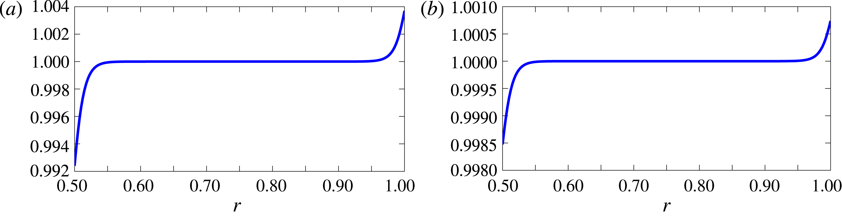
Plot of (a)
 $\unicode[STIX]{x1D70C}_{nbl}(h)/\widehat{\unicode[STIX]{x1D70C}_{0}}(r)$
and (b)
 $c_{nbl}(h)/\widehat{c_{0}}(r)$
, showing they can be approximated by a constant for a flow with an exponential boundary layer of displacement thickness
 $\unicode[STIX]{x1D700}=0.02$
(with
 $U_{\unicode[STIX]{x1D703}}=0.5$
).

Due to the complicated form of both
 $P_{1}$
and
 $V_{1}$
, it will be useful to make a simplification before calculating
 $P_{1}(0)$
and
 $V_{1}(0)$
. For the base flow, empirically
 $\widehat{\unicode[STIX]{x1D70C}_{0}}=\unicode[STIX]{x1D70C}_{nbl}+O(\unicode[STIX]{x1D6FF}^{\star })$
and
 $\widehat{c_{0}}=c_{nbl}+O(\unicode[STIX]{x1D6FF}^{\star })$
, where
 $\unicode[STIX]{x1D6FF}^{\star }=o(\unicode[STIX]{x1D6FF})$
. In figure 1, this can be seen by plotting the density ratio
 $\unicode[STIX]{x1D70C}_{nbl}(h)/\widehat{\unicode[STIX]{x1D70C}_{0}}$
and speed of sound ratio
 $c_{nbl}(h)/\widehat{c_{0}}(r)$
for an exponential boundary layer with displacement thickness
 $\unicode[STIX]{x1D700}=0.02$
and
 $U_{\unicode[STIX]{x1D703}}=0.5$
. Since the effective impedance is only calculated to
 $O(\unicode[STIX]{x1D6FF})$
, then the ratios
 $\unicode[STIX]{x1D70C}_{nbl}/\widehat{\unicode[STIX]{x1D70C}_{0}}$
and
 $c_{nbl}^{2}/\widehat{c_{0}}^{2}$
can be approximated by
 $1$
in (C 1), (C 2), (C 3) and (C 4). This will be particularly useful in simplifying the pressure term. This approximation is referred to as the ‘simplified’ modified Myers for swirling flow, as opposed to the ‘full’ modified Myers.
3.5 Solution at the inner duct wall
Finally,
 $P(0)$
and
 $V(0)$
have to be evaluated at the duct wall to be related to the pressure and normal velocity of the flow without a boundary layer at the duct wall,
 $P_{\infty }^{h}$
and
 $V_{\infty }^{h}$
, to finally complete the derivation of the modified Myers boundary condition.
3.5.1 Normal velocity
From (3.8), (3.13) and (C 1) the normal velocity at the wall is found to be
 $$\begin{eqnarray}V(0)=-\frac{\unicode[STIX]{x1D714}}{\unicode[STIX]{x1D6EC}_{nbl}(h)}V_{\infty }^{h}-\unicode[STIX]{x1D6FF}\unicode[STIX]{x1D714}C_{h}+O(\unicode[STIX]{x1D6FF}^{2}).\end{eqnarray}$$
A simplified form for
 $C_{h}$
is calculated from inserting the expression for
 $P_{0}(y)$
from (3.13) into (C 3) and then using the simplifications from § 3.4. The normal velocity at the duct wall is then given by:
 $$\begin{eqnarray}\displaystyle \frac{V(0)}{V_{\infty }^{h}} & = & \displaystyle -\frac{\unicode[STIX]{x1D714}}{\unicode[STIX]{x1D6EC}_{nbl}(h)}-\unicode[STIX]{x1D6FF}\text{i}\frac{\unicode[STIX]{x1D714}\left(k^{2}+\displaystyle \frac{m^{2}}{h^{2}}\right)}{\unicode[STIX]{x1D70C}_{nbl}(h)\unicode[STIX]{x1D6EC}_{nbl}^{2}(h)}\frac{P_{\infty }^{h}}{V_{\infty }^{h}}\int _{0}^{\infty }\left(1-\frac{\unicode[STIX]{x1D6EC}_{nbl}^{2}(h)}{\unicode[STIX]{x1D6EC}_{h}^{2}}\right)\text{d}y\nonumber\\ \displaystyle & & \displaystyle +\,\unicode[STIX]{x1D6FF}\frac{\unicode[STIX]{x1D714}\left(k^{2}+\displaystyle \frac{m^{2}}{h^{2}}\right)(U_{\unicode[STIX]{x1D703}}^{nbl})^{2}}{h\unicode[STIX]{x1D6EC}_{nbl}^{3}(h)}\int _{0}^{\infty }\frac{\unicode[STIX]{x1D6EC}_{nbl}^{2}(h)}{\unicode[STIX]{x1D6EC}_{h}^{2}}\left[1-\frac{U_{\unicode[STIX]{x1D703}}^{2}}{(U_{\unicode[STIX]{x1D703}}^{nbl})^{2}}\right]\text{d}y\nonumber\\ \displaystyle & & \displaystyle -\,\unicode[STIX]{x1D6FF}\frac{2m\unicode[STIX]{x1D714}U_{\unicode[STIX]{x1D703}}^{nbl}}{h^{2}\unicode[STIX]{x1D6EC}_{nbl}^{2}(h)}\int _{0}^{\infty }1-\frac{U_{\unicode[STIX]{x1D703}}\unicode[STIX]{x1D6EC}_{nbl}(h)}{U_{\unicode[STIX]{x1D703}}^{nbl}\unicode[STIX]{x1D6EC}_{h}}\,\text{d}y+O(\unicode[STIX]{x1D6FF}^{2}).\end{eqnarray}$$
3.5.2 Pressure
Similarly, from (3.8), (3.13) and (C 2) the pressure at the wall is found to be
 $$\begin{eqnarray}\displaystyle \frac{P(0)}{V_{\infty }^{h}}=\frac{P_{\infty }^{h}}{V_{\infty }^{h}}-\frac{\text{i}}{h\unicode[STIX]{x1D6EC}_{nbl}(h)}\int _{0}^{\infty }\widehat{\unicode[STIX]{x1D70C}_{0}}(U_{\unicode[STIX]{x1D703}}^{2})_{y}\,\text{d}y+\frac{\unicode[STIX]{x1D6FF}D_{h}}{V_{\infty }^{h}}+O(\unicode[STIX]{x1D6FF}^{2}). & & \displaystyle\end{eqnarray}$$
 $D_{h}$
is calculated by inserting the definition of
 $P_{0}(y)$
and
 $V_{1}(y)$
into (C 4) and using the simplifications from § 3.4. After some algebra
 $\unicode[STIX]{x1D6FF}P^{h}=\unicode[STIX]{x1D6FF}D_{h}/V_{\infty }^{h}$
can be calculated, and it is given by (C 5) in appendix C.
3.6 The modified Myers boundary condition at the inner wall
Having calculated
 $P(0)$
and
 $V(0)$
at the inner wall, the effective impedance can be evaluated. Let
 $Z_{h}=-P(h)/V(h)$
be the true impedance at the duct wall, and
 $Z_{eff}^{h}=-P_{\infty }^{h}/V_{\infty }^{h}$
be the effective impedance needed by the flow without a boundary layer. The bounded integrals are written in terms of
 $r$
instead of
 $y$
. The true impedance reads
 $$\begin{eqnarray}Z_{h}=-\frac{P(h)}{V(h)}=-\frac{\displaystyle \frac{P(h)}{V_{\infty }^{h}}}{\displaystyle \frac{V(h)}{V_{\infty }^{h}}}=\frac{Z_{eff}^{h}+\displaystyle \frac{\text{i}}{h\unicode[STIX]{x1D6EC}_{nbl}(h)}\int _{h}^{r_{m}}\widehat{\unicode[STIX]{x1D70C}_{0}}(U_{\unicode[STIX]{x1D703}}^{2})_{r}\,\text{d}r-Z_{eff}^{h}\unicode[STIX]{x1D6FF}I_{1}^{h}-\unicode[STIX]{x1D6FF}I_{2}^{h}}{-\displaystyle \frac{\unicode[STIX]{x1D714}}{\unicode[STIX]{x1D6EC}_{nbl}(h)}+Z_{eff}^{h}\unicode[STIX]{x1D6FF}J_{1}^{h}+\unicode[STIX]{x1D6FF}J_{2}^{h}}+O(\unicode[STIX]{x1D6FF}^{2}),\end{eqnarray}$$
where
 $$\begin{eqnarray}\displaystyle \unicode[STIX]{x1D6FF}J_{1}^{h} & = & \displaystyle \frac{\text{i}\unicode[STIX]{x1D714}\left(k^{2}+\displaystyle \frac{m^{2}}{h^{2}}\right)}{\unicode[STIX]{x1D70C}_{nbl}(h)\unicode[STIX]{x1D6EC}_{nbl}^{2}(h)}\int _{h}^{r_{m}}1-\frac{\unicode[STIX]{x1D6EC}_{nbl}^{2}(h)}{\unicode[STIX]{x1D6EC}_{h}^{2}}\,\text{d}r,\end{eqnarray}$$
 $$\begin{eqnarray}\displaystyle \unicode[STIX]{x1D6FF}J_{2}^{h} & = & \displaystyle \frac{\unicode[STIX]{x1D714}\left(k^{2}+\displaystyle \frac{m^{2}}{h^{2}}\right)(U_{\unicode[STIX]{x1D703}}^{nbl})^{2}}{h\unicode[STIX]{x1D6EC}_{nbl}^{3}(h)}\int _{h}^{r_{m}}\frac{\unicode[STIX]{x1D6EC}_{nbl}^{2}(h)}{\unicode[STIX]{x1D6EC}_{h}^{2}}\left[1-\frac{U_{\unicode[STIX]{x1D703}}^{2}}{(U_{\unicode[STIX]{x1D703}}^{nbl})^{2}}\right]\text{d}r\nonumber\\ \displaystyle & & \displaystyle -\,\frac{2m\unicode[STIX]{x1D714}U_{\unicode[STIX]{x1D703}}^{nbl}}{h^{2}\unicode[STIX]{x1D6EC}_{nbl}^{2}(h)}\int _{h}^{r_{m}}1-\frac{U_{\unicode[STIX]{x1D703}}\unicode[STIX]{x1D6EC}_{nbl}(h)}{U_{\unicode[STIX]{x1D703}}^{nbl}\unicode[STIX]{x1D6EC}_{h}}\,\text{d}r,\end{eqnarray}$$
 $$\begin{eqnarray}\displaystyle \unicode[STIX]{x1D6FF}I_{1}^{h} & = & \displaystyle \frac{2mU_{\unicode[STIX]{x1D703}}^{nbl}}{h^{2}\unicode[STIX]{x1D6EC}_{nbl}(h)}\int _{h}^{r_{m}}1-\frac{U_{\unicode[STIX]{x1D703}}\unicode[STIX]{x1D6EC}_{nbl}(h)}{U_{\unicode[STIX]{x1D703}}^{nbl}\unicode[STIX]{x1D6EC}_{h}}\,\text{d}r-\frac{\left(k^{2}+\displaystyle \frac{m^{2}}{h^{2}}\right)(U_{\unicode[STIX]{x1D703}}^{nbl})^{2}}{h\unicode[STIX]{x1D6EC}_{nbl}^{2}(h)}\int _{h}^{r_{m}}1-\frac{U_{\unicode[STIX]{x1D703}}^{2}\unicode[STIX]{x1D6EC}_{nbl}^{2}(h)}{(U_{\unicode[STIX]{x1D703}}^{nbl})^{2}\unicode[STIX]{x1D6EC}_{h}^{2}}\,\text{d}r,\nonumber\\ \displaystyle & & \displaystyle\end{eqnarray}$$
and
 $$\begin{eqnarray}\displaystyle \unicode[STIX]{x1D6FF}I_{2}^{h} & = & \displaystyle \frac{\text{i}\unicode[STIX]{x1D70C}_{nbl}(h)(U_{\unicode[STIX]{x1D703}}^{nbl})^{4}}{h^{2}c_{nbl}^{2}(h)\unicode[STIX]{x1D6EC}_{nbl}(h)}\int _{h}^{r_{m}}\frac{U_{\unicode[STIX]{x1D703}}^{2}}{(U_{\unicode[STIX]{x1D703}}^{nbl})^{2}}\left[1-\frac{U_{\unicode[STIX]{x1D703}}^{2}}{(U_{\unicode[STIX]{x1D703}}^{nbl})^{2}}\right]\text{d}r\nonumber\\ \displaystyle & & \displaystyle +\,\frac{4\text{i}\unicode[STIX]{x1D70C}_{nbl}(h)(U_{\unicode[STIX]{x1D703}}^{nbl})^{2}}{h^{2}\unicode[STIX]{x1D6EC}_{nbl}(h)}\int _{h}^{r_{m}}1-\frac{U_{\unicode[STIX]{x1D703}}^{2}}{(U_{\unicode[STIX]{x1D703}}^{nbl})^{2}}\,\text{d}r-\text{i}\unicode[STIX]{x1D70C}_{nbl}(h)\unicode[STIX]{x1D6EC}_{nbl}(h)\int _{h}^{r_{m}}1-\frac{\unicode[STIX]{x1D6EC}_{h}^{2}}{\unicode[STIX]{x1D6EC}_{nbl}^{2}(h)}\,\text{d}r\nonumber\\ \displaystyle & & \displaystyle -\,\frac{4\text{i}m\unicode[STIX]{x1D70C}_{nbl}(h)(U_{\unicode[STIX]{x1D703}}^{nbl})^{3}}{h^{3}\unicode[STIX]{x1D6EC}_{nbl}^{2}(h)}\int _{h}^{r_{m}}\frac{U_{\unicode[STIX]{x1D703}}\unicode[STIX]{x1D6EC}_{nbl}(h)}{U_{\unicode[STIX]{x1D703}}^{nbl}\unicode[STIX]{x1D6EC}_{h}}\left[1-\frac{U_{\unicode[STIX]{x1D703}}^{2}}{(U_{\unicode[STIX]{x1D703}}^{nbl})^{2}}\right]\text{d}r\nonumber\\ \displaystyle & & \displaystyle +\,\frac{\text{i}\left(k^{2}+\displaystyle \frac{m^{2}}{h^{2}}\right)\unicode[STIX]{x1D70C}_{nbl}(h)(U_{\unicode[STIX]{x1D703}}^{nbl})^{4}}{h^{2}\unicode[STIX]{x1D6EC}_{nbl}^{3}(h)}\int _{h}^{r_{m}}\frac{U_{\unicode[STIX]{x1D703}}^{2}\unicode[STIX]{x1D6EC}_{nbl}^{2}(h)}{(U_{\unicode[STIX]{x1D703}}^{nbl})^{2}\unicode[STIX]{x1D6EC}_{h}^{2}}\left[1-\frac{U_{\unicode[STIX]{x1D703}}^{2}}{(U_{\unicode[STIX]{x1D703}}^{nbl})^{2}}\right]\text{d}r\nonumber\\ \displaystyle & & \displaystyle -\,\frac{2\text{i}m\unicode[STIX]{x1D70C}_{nbl}(h)(U_{\unicode[STIX]{x1D703}}^{nbl})^{3}}{h^{3}\unicode[STIX]{x1D6EC}_{nbl}^{2}(h)}\int _{h}^{r_{m}}1-\frac{U_{\unicode[STIX]{x1D703}}\unicode[STIX]{x1D6EC}_{nbl}(h)}{U_{\unicode[STIX]{x1D703}}^{nbl}\unicode[STIX]{x1D6EC}_{h}}\,\text{d}r.\end{eqnarray}$$
Hence, to first order the effective impedance is finally
 $$\begin{eqnarray}\displaystyle Z_{eff}^{h}=-\frac{\unicode[STIX]{x1D714}\left(Z_{h}+\displaystyle \frac{\text{i}}{h\unicode[STIX]{x1D714}}\int _{h}^{r_{m}}\widehat{\unicode[STIX]{x1D70C}_{0}}(U_{\unicode[STIX]{x1D703}}^{2})_{r}\,\text{d}r\right)+\unicode[STIX]{x1D6EC}_{nbl}(h)\unicode[STIX]{x1D6FF}I_{2}^{h}+Z_{h}\unicode[STIX]{x1D6EC}_{nbl}(h)\unicode[STIX]{x1D6FF}J_{2}^{h}}{\unicode[STIX]{x1D6EC}_{nbl}(h)(1-\unicode[STIX]{x1D6FF}I_{1}^{h}-Z_{h}\unicode[STIX]{x1D6FF}J_{1}^{h})}.\end{eqnarray}$$
The boundary condition at the outer wall is provided in appendix D.
4 Useful limits of the modified Myers boundary condition
It is worth computing the boundary condition in some useful limits. Firstly, it is clear that in the limit of an infinitely thin boundary layer with
 $\unicode[STIX]{x1D6FF}=0$
, the boundary condition from Masson et al. (Reference Masson, Mathews, Moreau, Posson and Brambley2017) is recovered, i.e. in the limit of
 $\unicode[STIX]{x1D6FF}\rightarrow 0$
, (3.26) tends to (2.19) provided that the slight assumption of constant density in the boundary layer is assumed.
4.1 Limit in hard walls
Next, the specific case of a hard wall duct is considered, namely
 $Z=\infty$
. By taking the limit as
 $Z\rightarrow \infty$
in (3.26) and (D 1), the effective impedance is
 $$\begin{eqnarray}Z_{eff}^{h}=\frac{\unicode[STIX]{x1D714}+\unicode[STIX]{x1D6EC}_{nbl}(h)\unicode[STIX]{x1D6FF}J_{2}^{h}}{\unicode[STIX]{x1D6EC}_{nbl}(h)\unicode[STIX]{x1D6FF}J_{1}^{h}}\quad \text{and}\quad Z_{eff}^{1}=\frac{\unicode[STIX]{x1D714}-\unicode[STIX]{x1D6EC}_{nbl}(1)\unicode[STIX]{x1D6FF}J_{2}^{d}}{\unicode[STIX]{x1D6EC}_{nbl}(1)\unicode[STIX]{x1D6FF}J_{1}^{d}}.\end{eqnarray}$$
Thus, the effective impedance is a large purely imaginary value but non-infinite (since
 $\unicode[STIX]{x1D6FF}J_{2}$
is real and
 $\unicode[STIX]{x1D6FF}J_{1}$
is purely imaginary and non-zero). This is exactly the same situation as when the swirl was zero in Brambley (Reference Brambley2011).
4.2 Limit in no swirl
Finally, it is worth checking that in the limit of no swirl the effective impedance from Brambley (Reference Brambley2011) and Khamis & Brambley (Reference Khamis and Brambley2016) is retrieved. They were derived at the outer wall. In that case,
 $\unicode[STIX]{x1D70C}_{nbl}(1)=1$
,
 $\unicode[STIX]{x1D6FF}J_{2}^{d}=\unicode[STIX]{x1D6FF}I_{1}^{d}=0$
,
 $$\begin{eqnarray}\unicode[STIX]{x1D6FF}J_{1}^{d}=\frac{\text{i}\unicode[STIX]{x1D714}(k^{2}+m^{2})}{\unicode[STIX]{x1D6EC}_{nbl}^{2}(1)}\int _{r_{m}}^{1}1-\frac{\unicode[STIX]{x1D6EC}_{nbl}^{2}(1)}{\unicode[STIX]{x1D6EC}_{1}^{2}}\,\text{d}r\quad \text{and}\quad \unicode[STIX]{x1D6FF}I_{2}^{d}=\text{i}\unicode[STIX]{x1D6EC}_{nbl}(1)\int _{r_{m}}^{1}1-\frac{\unicode[STIX]{x1D6EC}_{1}^{2}}{\unicode[STIX]{x1D6EC}_{nbl}^{2}(1)}\,\text{d}r.\end{eqnarray}$$
The effective impedance is then given by
 $$\begin{eqnarray}Z_{eff}^{1}=\frac{-\unicode[STIX]{x1D714}Z_{1}-\unicode[STIX]{x1D6EC}_{nbl}(1)\unicode[STIX]{x1D6FF}I_{2}^{d}}{\unicode[STIX]{x1D6EC}_{nbl}(1)(1-Z_{1}\unicode[STIX]{x1D6FF}J_{1}^{d})},\end{eqnarray}$$
which agrees exactly with the result in Brambley (Reference Brambley2011) once the opposite Fourier transform sign convention (
 $\unicode[STIX]{x1D714}\rightarrow -\unicode[STIX]{x1D714}$
,
 $k\rightarrow -k$
,
 $m\rightarrow -m$
) is used.
5 Extending the validity of the new boundary condition
Next, the usefulness of the boundary condition is extended to arbitrary, radially varying profiles. The boundary condition also easily extends in the case of grazing flow with non-zero slip flow at the boundary (
 $U_{x}(h),U_{\unicode[STIX]{x1D703}}(h)\neq 0$
), which Aurégan, Starobinski & Pagneux (Reference Aurégan, Starobinski and Pagneux2001) showed was needed to model surface roughness. Essentially,
 $\unicode[STIX]{x1D714}$
is replaced by
 $-\unicode[STIX]{x1D6EC}(h)$
in (3.26) and the associated delta integrals.
For conciseness, only the flow at the inner wall will be considered, with a very similar result holding at the outer wall which is given in appendix E. The change of variables
 $r=h+\unicode[STIX]{x1D6FF}y$
will again be used. The only problem with the analysis in § 3 is that now the limits
 $U_{x}(y)$
and
 $U_{\unicode[STIX]{x1D703}}(y)$
are not defined as
 $y\rightarrow \infty$
(i.e. outside of the boundary layer), due to the radial variation in the flow. To overcome this, we introduce
 $$\begin{eqnarray}\widehat{U_{x}}(y)=\frac{U_{x}^{nbl}(h)U_{x}(y)}{U_{x}^{nbl}(y)}\quad \text{and}\quad \widehat{U_{\unicode[STIX]{x1D703}}}(y)=\frac{U_{\unicode[STIX]{x1D703}}^{nbl}(h)U_{\unicode[STIX]{x1D703}}(y)}{U_{\unicode[STIX]{x1D703}}^{nbl}(y)},\end{eqnarray}$$
so that
 $\widehat{U_{x}}(y)$
and
 $\widehat{U_{\unicode[STIX]{x1D703}}}(y)$
have limits as
 $y\rightarrow \infty$
. Similarly,
 $\widehat{U_{x}}(r)$
and
 $\widehat{U_{\unicode[STIX]{x1D703}}}(r)$
can be defined. The results
 $$\begin{eqnarray}\frac{U_{\unicode[STIX]{x1D703}}^{nbl}(h)}{U_{\unicode[STIX]{x1D703}}^{nbl}(y)}=1-\unicode[STIX]{x1D6FF}y\frac{(U_{\unicode[STIX]{x1D703}}^{nbl})^{\prime }(h)}{U_{\unicode[STIX]{x1D703}}^{nbl}(h)}+O(\unicode[STIX]{x1D6FF}^{2})\quad \text{and}\quad U_{\unicode[STIX]{x1D703}}(y)=U_{\unicode[STIX]{x1D703}}(h)+\unicode[STIX]{x1D6FF}yU_{\unicode[STIX]{x1D703}}^{\prime }(h)+O(\unicode[STIX]{x1D6FF}^{2})=O(\unicode[STIX]{x1D6FF}),\end{eqnarray}$$
follow from Taylor expanding (in
 $\unicode[STIX]{x1D6FF}$
)
 $U_{\unicode[STIX]{x1D703}}^{nbl}$
and
 $U_{\unicode[STIX]{x1D703}}$
, with the latter equation following since
 $U_{\unicode[STIX]{x1D703}}(h)=0$
. Thus,
 $$\begin{eqnarray}\widehat{U_{\unicode[STIX]{x1D703}}}(y)=U_{\unicode[STIX]{x1D703}}(y)+O(\unicode[STIX]{x1D6FF}^{2}),\end{eqnarray}$$
and similarly
 $$\begin{eqnarray}\widehat{U_{x}}(y)=U_{x}(y)+O(\unicode[STIX]{x1D6FF}^{2}).\end{eqnarray}$$
Hence, we can effectively ignore the radial variations of the mean flow velocities in the boundary layer to first order. To first order,
 $U_{\unicode[STIX]{x1D703}}(y)$
,
 $U_{x}(y)$
and
 $\unicode[STIX]{x1D6EC}_{h}(y)$
can then be replaced by
 $\widehat{U_{\unicode[STIX]{x1D703}}}(y)$
,
 $\widehat{U_{x}}(y)$
and
 $\widehat{\unicode[STIX]{x1D6EC}_{h}}(y)=k\widehat{U_{x}}(y)+m\widehat{U_{\unicode[STIX]{x1D703}}}(y)/h-\unicode[STIX]{x1D714}$
respectively. These have limits of
 $U_{\unicode[STIX]{x1D703}}^{nbl}(h)$
,
 $U_{x}^{nbl}(h)$
and
 $\unicode[STIX]{x1D6EC}_{nbl}(h)=kU_{x}^{nbl}(h)+mU_{\unicode[STIX]{x1D703}}^{nbl}(h)/h-\unicode[STIX]{x1D714}$
respectively as
 $y\rightarrow \infty$
. Using the same method as in § 3 then gives the effective impedance at the inner wall as
 $$\begin{eqnarray}Z_{eff}^{h}=-\frac{\unicode[STIX]{x1D714}\left(Z_{h}+\displaystyle \frac{\text{i}}{h\unicode[STIX]{x1D714}}\int _{h}^{r_{m}}\widehat{\unicode[STIX]{x1D70C}_{0}}(\widehat{U_{\unicode[STIX]{x1D703}}}^{2})_{r}\,\text{d}r\right)+\unicode[STIX]{x1D6EC}_{nbl}(h)\unicode[STIX]{x1D6FF}I_{2}^{h}+Z_{h}\unicode[STIX]{x1D6EC}_{nbl}(h)\unicode[STIX]{x1D6FF}J_{2}^{h}}{\unicode[STIX]{x1D6EC}_{nbl}(h)(1-\unicode[STIX]{x1D6FF}I_{1}^{h}-Z_{h}\unicode[STIX]{x1D6FF}J_{1}^{h})},\end{eqnarray}$$
where the integrands of
 $\unicode[STIX]{x1D6FF}I$
and
 $\unicode[STIX]{x1D6FF}J$
in (3.25) instead involve terms of the form
 $$\begin{eqnarray}\frac{\widehat{U_{\unicode[STIX]{x1D703}}}(r)}{U_{\unicode[STIX]{x1D703}}^{nbl}(h)}\quad \text{and}\quad \frac{\widehat{\unicode[STIX]{x1D6EC}_{h}}(r)}{\unicode[STIX]{x1D6EC}_{nbl}(h)}.\end{eqnarray}$$
Finally, the relations
 $$\begin{eqnarray}\frac{\widehat{U_{\unicode[STIX]{x1D703}}}(r)}{U_{\unicode[STIX]{x1D703}}^{nbl}(h)}=\frac{U_{\unicode[STIX]{x1D703}}(r)}{U_{\unicode[STIX]{x1D703}}^{nbl}(r)}\quad \text{and}\quad \frac{\widehat{\unicode[STIX]{x1D6EC}_{h}}(r)}{\unicode[STIX]{x1D6EC}_{nbl}(h)}=\frac{kU_{x}(r)+mU_{\unicode[STIX]{x1D703}}(r)/h-\unicode[STIX]{x1D714}}{kU_{x}^{nbl}(r)+mU_{\unicode[STIX]{x1D703}}^{nbl}(r)/h-\unicode[STIX]{x1D714}}+O(\unicode[STIX]{x1D6FF}),\end{eqnarray}$$
are used to give the final boundary condition in appendix E.
6 Assessment of the modified Myers boundary condition in swirling flow
The new boundary condition is first assessed by checking its error behaviour with boundary layer thickness, which should be quadratic. The exact value of the impedance
 $Z_{eff}^{h}=-P_{nbl}(h)/V_{nbl}(h)$
at the inner wall is compared with the calculated value from the modified Myers boundary condition in (3.26) for constant axial and swirling flow. The analysis is then repeated at the outer wall, but for radially varying axial and swirling flow. In both cases, several values of
 $k$
are chosen, and the boundary layer thickness is varied to produce similar figures to Khamis & Brambley (Reference Khamis and Brambley2016, figure 1). Instead, the boundary layer thickness could be fixed and the whole
 $k$
plane considered, as in Khamis & Brambley (Reference Khamis and Brambley2016, figure 2).
6.1 Boundary layer profile
A duct where the inner wall is given by
 $h=0.5$
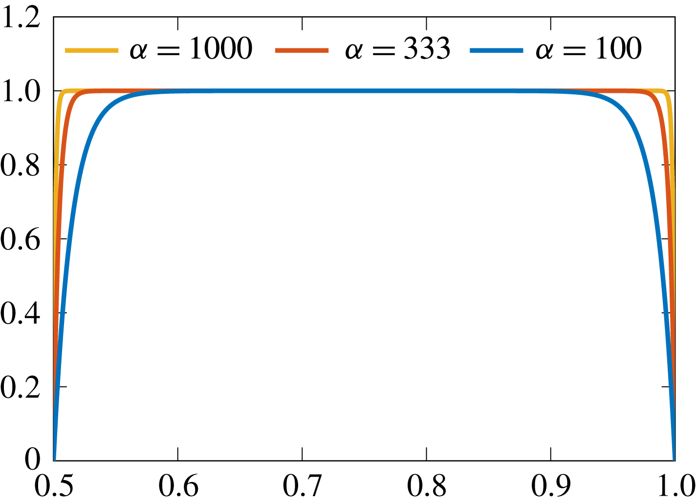
is considered. An exponential boundary layer profile of normalised shape
 $$\begin{eqnarray}L_{\unicode[STIX]{x1D6FC}}^{exp}(r)=1-\text{e}^{-\unicode[STIX]{x1D6FC}(r-h)}-\text{e}^{-\unicode[STIX]{x1D6FC}(1-r)},\end{eqnarray}$$
with different values of
 $\unicode[STIX]{x1D6FC}$
is selected. In figure 2, the boundary layer profile for
 $\unicode[STIX]{x1D6FC}=100$
,
 $\unicode[STIX]{x1D6FC}=333$
and
 $\unicode[STIX]{x1D6FC}=1000$
are plotted. The flow with and without the boundary layer are related by
 $U_{x}(r)=U_{x}^{nbl}L_{\unicode[STIX]{x1D6FC}}^{exp}(r)$
and
 $U_{\unicode[STIX]{x1D703}}(r)=U_{\unicode[STIX]{x1D703}}^{nbl}L_{\unicode[STIX]{x1D6FC}}^{exp}(r)$
. Given a boundary layer profile, the displacement thickness at each duct wall is given by
 $$\begin{eqnarray}\unicode[STIX]{x1D700}^{h}=2\int _{h}^{r_{m}}1-\frac{U_{x}(r)}{U_{x}^{nbl}(r)}\,\text{d}r\quad \text{and}\quad \unicode[STIX]{x1D700}^{1}=2\int _{r_{m}}^{1}1-\frac{U_{x}(r)}{U_{x}^{nbl}(r)}\,\text{d}r,\end{eqnarray}$$
which is proportional to the boundary layer thickness.
Boundary layer profiles
 $L_{\unicode[STIX]{x1D6FC}}^{exp}(r)$
in (6.1) for different values of
 $\unicode[STIX]{x1D6FC}$
.

In § 7.2, other boundary layer profiles are considered, such as a polynomial boundary layer to model a laminar boundary layer rather than a turbulent boundary layer.
6.2 Assessment at the inner wall for swirl with constant azimuthal velocity
The modified Myers boundary condition is now assessed at the inner wall. Different values of
 $k$
are considered (
 $k=\pm 1$
and
 $k=\pm (1+\text{i})$
), with the other parameters chosen as
 $\unicode[STIX]{x1D714}=5$
,
 $h=0.5$
,
 $m=1$
,
 $U_{x}^{nbl}=0.5$
and
 $U_{\unicode[STIX]{x1D703}}^{nbl}=0.5$
for a canonical example. An exponential boundary layer profile is specified, but only near
 $r=h$
. A boundary condition is imposed at the outer wall of
 $P(1)/V(1)=P_{nbl}(1)/V_{nbl}(1)=Z=1-\text{i}$
, with the choice of
 $Z$
arbitrary. From using this boundary condition and the governing equations (2.14) and (2.15) for swirling flow without a boundary layer (and arbitrarily specifying
 $V(1)$
to be a constant
 $c$
) the exact value of
 $Z_{eff}^{h}=-P_{nbl}(h)/V_{nbl}(h)$
can be computed, since the constant drops out. The swirling flow with a boundary layer is then considered to compute
 $P(h)/V(h)$
, and then let
 $$\begin{eqnarray}Z_{eff}^{h,\star }=\frac{-\unicode[STIX]{x1D714}\left(-\displaystyle \frac{P(h)}{V(h)}+\frac{\text{i}}{h\unicode[STIX]{x1D714}}\int _{h}^{r_{m}}\widehat{\unicode[STIX]{x1D70C}_{0}}(U_{\unicode[STIX]{x1D703}}^{2})_{r}\,\text{d}r\right)+\unicode[STIX]{x1D6EC}_{nbl}(h)\unicode[STIX]{x1D6FF}I_{2}^{h}-\displaystyle \frac{P(h)}{V(h)}\unicode[STIX]{x1D6EC}_{nbl}(h)\unicode[STIX]{x1D6FF}J_{2}^{h}}{\unicode[STIX]{x1D6EC}_{nbl}(h)\left(1-\unicode[STIX]{x1D6FF}I_{1}^{h}+\displaystyle \frac{P(h)}{V(h)}\unicode[STIX]{x1D6FF}J_{1}^{h}\right)},\end{eqnarray}$$
where
 $\unicode[STIX]{x1D6FF}I_{l}^{h}$
and
 $\unicode[STIX]{x1D6FF}J_{l}^{h}$
are given in (3.25). The relative error
 $|Z_{eff}^{h,\star }/Z_{eff}^{h}-1|$
is plotted against displacement thickness
 $\unicode[STIX]{x1D700}^{h}$
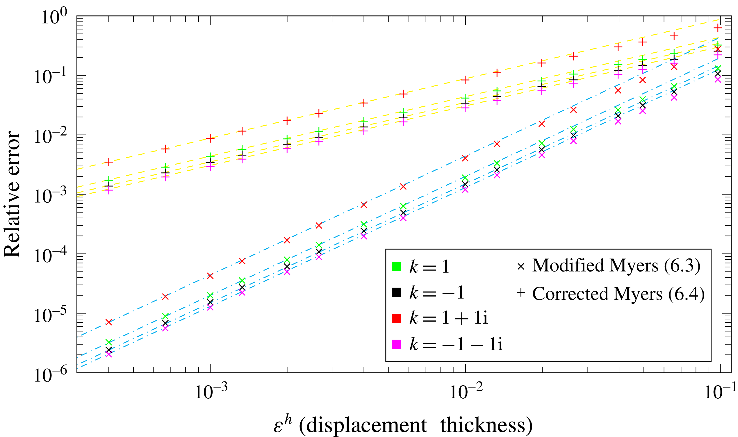
with crosses in figure 3.
Inner wall, constant flow. Plot of the relative error of the modified Myers condition
 $|Z_{eff}^{h,\star }/Z_{eff}^{h}-1|$
(crosses) and corrected Myers condition
 $|Z_{eff}^{h,\dagger }/Z_{eff}^{h}-1|$
(pluses) against displacement thickness
 $\unicode[STIX]{x1D700}^{h}$
. Different values of
 $k$
are considered, with the other parameters
 $\unicode[STIX]{x1D714}=5$
,
 $h=0.5$
,
 $m=1$
,
 $U_{x}^{nbl}=0.5$
and
 $U_{\unicode[STIX]{x1D703}}^{nbl}=0.5$
. Yellow dashed lines: gradient
 $1$
(zero-order solution); cyan dot-dashed lines: gradient
 $2$
(first-order solution).

The corrected Myers boundary condition is also considered, with
 $$\begin{eqnarray}Z_{eff}^{h,\dagger }=\frac{\unicode[STIX]{x1D714}\left(\displaystyle \frac{P(h)}{V(h)}-\frac{\text{i}}{\unicode[STIX]{x1D714}}\int _{h}^{r_{m}}\widehat{\unicode[STIX]{x1D70C}_{0}}(U_{\unicode[STIX]{x1D703}}^{2})_{r}\,\text{d}r\right)}{\unicode[STIX]{x1D6EC}_{nbl}(h)},\end{eqnarray}$$
and the relative error
 $|Z_{eff}^{h,\dagger }/Z_{eff}^{h}-1|$
is plotted against displacement thickness in figure 3 with pluses. From the figure, it is seen that the relative error for the corrected Myers boundary condition is linear as expected (with gradient
 $1$
, dashed yellow line). The relative error for the modified Myers boundary condition is seen to be quadratic (with gradient
 $2$
, dot-dashed cyan line) as expected.
6.3 Assessment at the outer wall with radially varying swirl
The boundary condition is now assessed at the outer wall, but with a radially varying swirling flow
 $U_{x}^{nbl}(r)=0.6-0.2r$
and
 $U_{\unicode[STIX]{x1D703}}^{nbl}(r)=0.3r+0.2/r$
, which is a representative test case. Different values of
 $k$
are considered (
 $k=3$
,
 $k=-5$
,
 $k=3+2\text{i}$
and
 $k=-1-\text{i}$
), with the other parameters
 $\unicode[STIX]{x1D714}=10$
,
 $h=0.5$
and
 $m=3$
. An exponential boundary layer profile is specified, but only near
 $r=1$
. The boundary condition at the inner wall is set as
 $-P(h)/V(h)=-P_{nbl}(h)/V_{nbl}(h)=Z=1-\text{i}$
, with
 $Z$
again arbitrary. From using this boundary condition and the governing equations
 $P_{nbl}(1)$
and
 $V_{nbl}(1)$
can be calculated by considering a swirling flow with no boundary layer, which allows the exact calculation of
 $Z_{eff}^{1}$
. By considering the same governing equation but with the swirling flow having the exponential boundary layer,
 $P(1)$
and
 $V(1)$
can be calculated. This allows the computation of
 $$\begin{eqnarray}Z_{eff}^{1,\star }=\frac{-\unicode[STIX]{x1D714}\left(\displaystyle \frac{P(1)}{V(1)}+\frac{\text{i}}{\unicode[STIX]{x1D714}}\int _{r_{m}}^{1}\widehat{\unicode[STIX]{x1D70C}_{0}}(\widehat{U_{\unicode[STIX]{x1D703}}}^{2})_{r}\,\text{d}r\right)-\unicode[STIX]{x1D6EC}_{nbl}(1)\unicode[STIX]{x1D6FF}I_{2}^{d}+\displaystyle \frac{P(1)}{V(1)}\unicode[STIX]{x1D6EC}_{nbl}(1)\unicode[STIX]{x1D6FF}J_{2}^{d}}{\unicode[STIX]{x1D6EC}_{nbl}(1)\left(1+\unicode[STIX]{x1D6FF}I_{1}^{d}-\displaystyle \frac{P(1)}{V(1)}\unicode[STIX]{x1D6FF}J_{1}^{d}\right)},\end{eqnarray}$$
where
 $\unicode[STIX]{x1D6FF}I_{l}^{d}$
and
 $\unicode[STIX]{x1D6FF}J_{l}^{d}$
can be found in appendix E. The relative error
 $|Z_{eff}^{1,\star }/Z_{eff}^{1}-1|$
is plotted against displacement thickness
 $\unicode[STIX]{x1D700}^{1}$
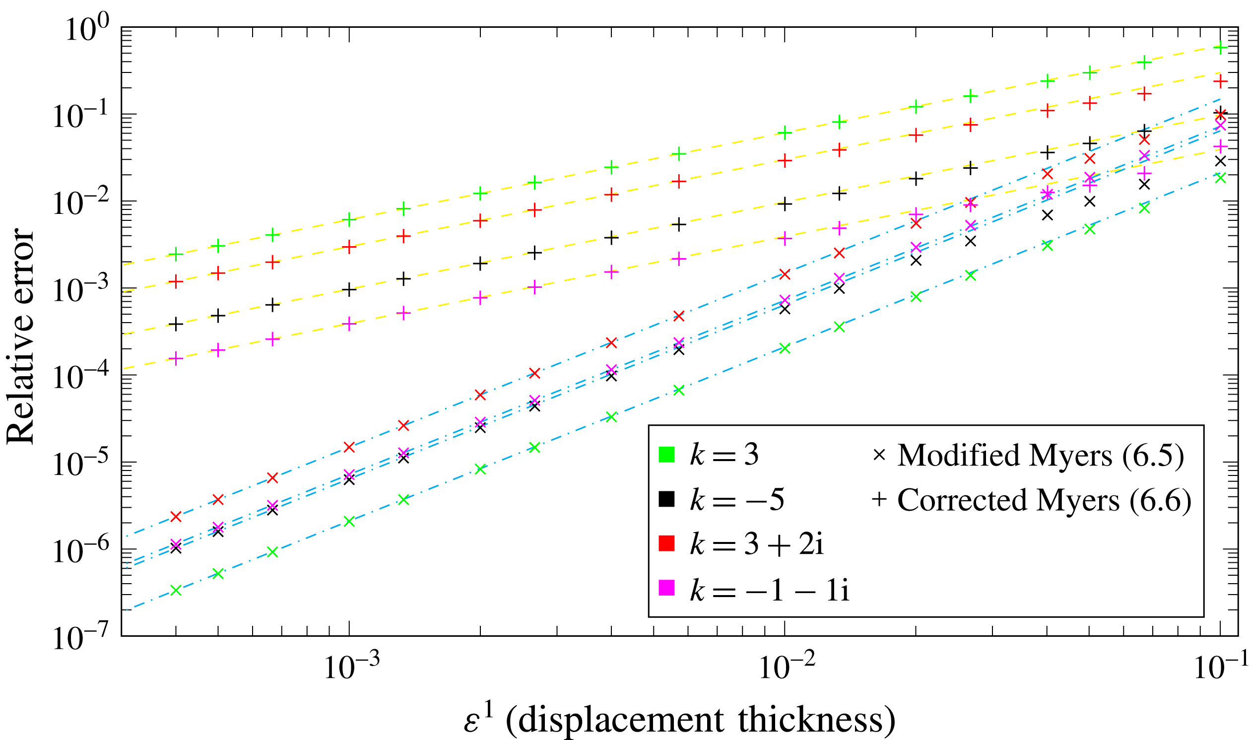
with crosses in figure 4.
Outer wall, varying flow. Plot of the relative error of the modified Myers condition
 $|Z_{eff}^{1,\star }/Z_{eff}^{1}-1|$
(crosses) and corrected Myers condition
 $|Z_{eff}^{1,\dagger }/Z_{eff}^{1}-1|$
(pluses) against displacement thickness
 $\unicode[STIX]{x1D700}$
. Different values of
 $k$
are considered, with the other parameters
 $\unicode[STIX]{x1D714}=10$
,
 $h=0.5$
,
 $m=3$
,
 $U_{x}^{nbl}(r)=0.6-0.2r$
and
 $U_{\unicode[STIX]{x1D703}}^{nbl}(r)=0.3r+0.2/r$
. Yellow dashed lines: gradient
 $1$
(zero-order solution); cyan dot-dashed lines: gradient
 $2$
(first-order solution).

The corrected Myers boundary condition
 $$\begin{eqnarray}Z_{eff}^{1,\dagger }=-\frac{\unicode[STIX]{x1D714}\left(\displaystyle \frac{P(1)}{V(1)}+\frac{\text{i}}{\unicode[STIX]{x1D714}}\int _{r_{m}}^{1}\widehat{\unicode[STIX]{x1D70C}_{0}}(\widehat{U_{\unicode[STIX]{x1D703}}}^{2})_{r}\,\text{d}r\right)}{\unicode[STIX]{x1D6EC}_{nbl}(1)},\end{eqnarray}$$
is also considered, and the relative error
 $|Z_{eff}^{1,\dagger }/Z_{eff}^{1}-1|$
is plotted against displacement thickness in figure 4 with pluses. From figure 4 it is clear that the relative error for the corrected Myers boundary condition is linear as expected, while the relative error for the modified Myers boundary condition is quadratic as expected.
There are a couple of interesting features from when the flow varies radially in figure 4 compared to figure 3. Firstly, in figure 3 the relative error is squared when changing the boundary condition from the corrected Myers to the modified Myers. In figure 4 there is a more complex relation between the relatives errors. For example when
 $\unicode[STIX]{x1D700}^{1}=4\times 10^{-4}$
, when
 $k=3$
(green) the relative error for the corrected Myers boundary condition is
 $2\times 10^{-3}$
, and for the modified Myers boundary condition it is
 $3\times 10^{-7}$
, so the error has more than squared. However, when
 $k=-1-1\text{i}$
(pink) the relative error for the corrected Myers boundary condition is
 $1.5\times 10^{-4}$
and for the modified Myers it is
 $1.1\times 10^{-6}$
, so the error has not improved by so much. The different error behaviour for radially varying flow is believed to be caused by the approximations from § 5 to derive the boundary condition in the case of radially varying flow. It is possible that other derivations of this boundary condition might give different error behaviour.
Secondly, for a large boundary layer thickness and varying flow it is possible that the modified Myers boundary condition actually does worse than the corrected Myers boundary condition, as seen when
 $k=-1-1\text{i}$
(pink) for
 $\unicode[STIX]{x1D700}^{1}\geqslant 0.05$
. This is likely because the approximations in § 3.4 are not valid for large boundary layer thicknesses, and introduce a significant error.
7 Shape of the boundary layer
In this section, the modified Myers boundary condition is first considered for a piecewise linear boundary layer, especially for a hard-walled duct. Then, the effect of different boundary layer profiles are considered but with the same boundary layer displacement thickness, to investigate how important the shape of the profile is.
To investigate the effects of the sound attenuation the acoustic eigenvalues are calculated by rearranging equations (2.13) to give an eigenvalue problem of the form
 $$\begin{eqnarray}\unicode[STIX]{x1D63C}(\text{i}U,V,\text{i}W,P)^{\text{T}}=k\unicode[STIX]{x1D63D}(\text{i}U,V,\text{i}W,P)^{\text{T}},\end{eqnarray}$$
where the matrices
 $\unicode[STIX]{x1D63C}$
and
 $\unicode[STIX]{x1D63D}$
are the standard matrices defined in Posson & Peake (Reference Posson and Peake2013), Mathews & Peake (Reference Mathews and Peake2017) amongst others, and are given in appendix F. The boundary condition at each duct wall also depends on
 $k$
.
7.1 Piecewise linear boundary layer
For a piecewise linear boundary layer, the integrals
 $\unicode[STIX]{x1D6FF}I$
and
 $\unicode[STIX]{x1D6FF}J$
can be calculated analytically. A piecewise linear boundary layer is chosen since it has the simplest possible form, although the integrals can also be evaluated analytically in other cases such as for an exponential boundary layer.
Let the boundary layer thickness be
 $\unicode[STIX]{x1D6FF}$
, then the piecewise linear boundary layer profile is
 $$\begin{eqnarray}U_{x,\unicode[STIX]{x1D703}}(r)=\left\{\begin{array}{@{}ll@{}}U_{x,\unicode[STIX]{x1D703}}^{nbl}(r-h)/\unicode[STIX]{x1D6FF}\quad & h\leqslant r<h+\unicode[STIX]{x1D6FF}\\ U_{x,\unicode[STIX]{x1D703}}^{nbl}\quad & h+\unicode[STIX]{x1D6FF}\leqslant r<1-\unicode[STIX]{x1D6FF}\\ U_{x,\unicode[STIX]{x1D703}}^{nbl}(1-r)/\unicode[STIX]{x1D6FF}\quad & 1-\unicode[STIX]{x1D6FF}\leqslant r\leqslant 1\end{array}\right.\!.\end{eqnarray}$$
7.1.1 Non-swirling flow
In Khamis & Brambley (Reference Khamis and Brambley2016, equation (6.2) to
 $O(\unicode[STIX]{x1D6FF})$
), it was shown that for non-swirling flow with a piecewise linear boundary layer, the boundary condition to first order is given by
 $$\begin{eqnarray}\displaystyle & & \displaystyle P[\unicode[STIX]{x1D714}^{2}-kU_{x}(2\unicode[STIX]{x1D714}+\text{i}\unicode[STIX]{x1D6FF}^{1}Z_{1}m^{2})+k^{2}U_{x}^{2}-k^{3}(\text{i}\unicode[STIX]{x1D6FF}^{1}U_{x}Z_{1})]\nonumber\\ \displaystyle & & \displaystyle \quad -\,V\left[\unicode[STIX]{x1D714}^{2}Z_{1}-k\unicode[STIX]{x1D714}U_{x}(Z_{1}+\text{i}\unicode[STIX]{x1D6FF}^{1}\unicode[STIX]{x1D714})+k^{2}\frac{5\text{i}\unicode[STIX]{x1D6FF}^{1}\unicode[STIX]{x1D714}U_{x}^{2}}{3}-k^{3}\frac{2\text{i}\unicode[STIX]{x1D6FF}^{1}U_{x}^{3}}{3}\right]=0\quad \text{at }r=1,\quad\end{eqnarray}$$
 $$\begin{eqnarray}\displaystyle & & \displaystyle P[\unicode[STIX]{x1D714}^{2}-kU_{x}(2\unicode[STIX]{x1D714}+\text{i}\unicode[STIX]{x1D6FF}^{h}Z_{h}(m^{2}/h^{2}))+k^{2}U_{x}^{2}-k^{3}(\text{i}\unicode[STIX]{x1D6FF}^{h}U_{x}Z_{h})]\nonumber\\ \displaystyle & & \displaystyle \quad +\,V\left[\unicode[STIX]{x1D714}^{2}Z_{h}-k\unicode[STIX]{x1D714}U_{x}(Z_{h}+\text{i}\unicode[STIX]{x1D6FF}^{h}\unicode[STIX]{x1D714})+k^{2}\frac{5\text{i}\unicode[STIX]{x1D6FF}^{h}\unicode[STIX]{x1D714}U_{x}^{2}}{3}-k^{3}\frac{2\text{i}\unicode[STIX]{x1D6FF}^{h}U_{x}^{3}}{3}\right]=0\quad \text{at }r=h,\quad\end{eqnarray}$$
namely only involving polynomials in
 $k$
. The same result holds by calculating the integrals analytically in (3.26) and setting the swirl to be zero. As a result, to solve the eigenvalue problem the variables
 ${\dot{P}}=kP$
,
 $\ddot{P}=k{\dot{P}}$
,
 $\dddot{P}=k\ddot{P}$
,
 $\dot{V}=kV$
,
 $\ddot{V}=k\dot{V}$
and
 $\dddot{V}=k\ddot{V}$
are defined which allows us removing the eigenvalue from the boundary condition and instead solve the system
 $$\begin{eqnarray}\unicode[STIX]{x1D63C}^{\star }(U,V,W,P,{\dot{P}},\ddot{P},\dddot{P},\dot{V},\ddot{V},\dddot{V})^{\text{T}}=k\quad \unicode[STIX]{x1D63D}^{\star }(U,V,W,P,{\dot{P}},\ddot{P},\dddot{P},\dot{V},\ddot{V},\dddot{V})^{\text{T}}.\end{eqnarray}$$
To get the hard wall boundary conditions the impedances are set to infinity, while to recover the standard Myers boundary condition in no swirl the boundary layer thickness
 $\unicode[STIX]{x1D6FF}$
is set to zero.
7.1.2 Swirling flow with hard walls
For conciseness, only the boundary condition at the inner wall is considered. The modified Myers boundary condition is given by (4.1). For a piecewise linear boundary layer profile
 $$\begin{eqnarray}\unicode[STIX]{x1D6FF}J_{1}^{h}=\unicode[STIX]{x1D6FF}\frac{\text{i}\left(k^{2}+\displaystyle \frac{m^{2}}{h^{2}}\right)}{\unicode[STIX]{x1D70C}_{nbl}(h)\unicode[STIX]{x1D6EC}_{nbl}^{2}(h)}\left(kU_{x}^{nbl}+\frac{mU_{\unicode[STIX]{x1D703}}^{nbl}}{h}\right),\end{eqnarray}$$
and
 $$\begin{eqnarray}\displaystyle \unicode[STIX]{x1D6FF}J_{2}^{h} & = & \displaystyle \unicode[STIX]{x1D6FF}\frac{2m\unicode[STIX]{x1D714}^{2}U_{\unicode[STIX]{x1D703}}^{nbl}}{h^{2}\unicode[STIX]{x1D6EC}_{nbl}^{2}(h)}\frac{1}{(kU_{x}^{nbl}+mU_{\unicode[STIX]{x1D703}}^{nbl}/h)^{2}}\left[\unicode[STIX]{x1D6EC}_{nbl}(h)\log \left(-\frac{\unicode[STIX]{x1D6EC}_{nbl}(h)}{\unicode[STIX]{x1D714}}\right)-kU_{x}^{nbl}-\frac{mU_{\unicode[STIX]{x1D703}}^{nbl}}{h}\right]\nonumber\\ \displaystyle & & \displaystyle +\,\unicode[STIX]{x1D6FF}\frac{\unicode[STIX]{x1D714}\left(k^{2}+\displaystyle \frac{m^{2}}{h^{2}}\right)(U_{\unicode[STIX]{x1D703}}^{nbl})^{2}}{h\unicode[STIX]{x1D6EC}_{nbl}^{3}(h)}\unicode[STIX]{x1D6EC}_{nbl}(h)\nonumber\\ \displaystyle & & \displaystyle \times \left(\frac{1}{\unicode[STIX]{x1D714}}+\frac{\unicode[STIX]{x1D6EC}_{nbl}^{2}(h)-\unicode[STIX]{x1D714}^{2}+2\unicode[STIX]{x1D714}\unicode[STIX]{x1D6EC}_{nbl}(h)\log \left(-\displaystyle \frac{\unicode[STIX]{x1D6EC}_{nbl}(h)}{\unicode[STIX]{x1D714}}\right)}{(kU_{x}^{nbl}+mU_{\unicode[STIX]{x1D703}}^{nbl}/h)^{3}}\right),\end{eqnarray}$$
so
 $\unicode[STIX]{x1D6FF}J_{1}^{h}$
is a polynomial in
 $k$
, but
 $\unicode[STIX]{x1D6FF}J_{2}^{h}$
is not, due to the
 $\log (-\unicode[STIX]{x1D6EC}_{nbl}(h)/\unicode[STIX]{x1D714})$
terms. Log terms prevent the use of spectral methods to solve the problem.
However, provided the boundary layer thickness is small compared to the frequency, then
 $|\unicode[STIX]{x1D6FF}J_{2}^{h}|\ll \unicode[STIX]{x1D714}$
, and hence the boundary condition becomes approximately
 $$\begin{eqnarray}Z_{eff}^{h}\approx \frac{\unicode[STIX]{x1D714}}{\unicode[STIX]{x1D6EC}_{nbl}(h)\unicode[STIX]{x1D6FF}J_{1}^{h}}=\frac{\unicode[STIX]{x1D714}h^{3}\unicode[STIX]{x1D70C}_{nbl}(h)\unicode[STIX]{x1D6EC}_{nbl}(h)}{\unicode[STIX]{x1D6FF}\text{i}(k^{2}h^{2}+m^{2})(khU_{x}^{nbl}+mU_{\unicode[STIX]{x1D703}}^{nbl})},\end{eqnarray}$$
which is a polynomial in
 $k$
. This is referred to as the one term modified Myers boundary condition for hard walls in swirling flow. A third-order polynomial can then be used for the boundary condition, similar to (7.4). In the case of non-swirling flow, (7.8) becomes exact with
 $U_{\unicode[STIX]{x1D703}}^{nbl}=0$
, and the boundary condition in (7.4) is recovered for
 $Z_{h}=\infty$
.
Comparison of eigenmodes when
 $m=5$
,
 $\unicode[STIX]{x1D714}=10$
,
 $U_{x}^{nbl}=U_{\unicode[STIX]{x1D703}}^{nbl}=0.5$
,
 $h=0.5$
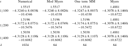
and hard walls. The eigenmodes from the fully resolved boundary layer (Numerical), the modified Myers (Mod Myers, equation (4.1)), the one term modified Myers (One term MM, equation (7.8)) and the original Myers boundary condition (Myers) are given at different displacement thicknesses
 $\unicode[STIX]{x1D700}$
. The final row is the number of the grid points,
 $\unicode[STIX]{x1D706}$
, needed for the discretisation.

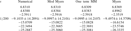
Comparison of eigenmodes for a counter-rotating mode
 $m=-6$
. The other details are as in table 1.

In table 1, the eigenmodes from a fully resolved boundary layer (second column), the modified Myers boundary condition (third column), one term modified Myers boundary condition (fourth column) and the Myers (fifth column) are compared for
 $m=5$
and
 $\unicode[STIX]{x1D714}=10$
. The eigenmodes are calculated at three different displacement thicknesses. Note that for hard walls the corrected Myers and the Myers boundary condition are equivalent.
The method used for calculating the eigenmodes for the nonlinear modified Myers boundary condition is given in the next section. For the fully resolved boundary layer, there are some difficulties in calculating the eigenmodes due to the discontinuities in the derivatives which appear in the operator in (F 1). This is dealt with by slightly smoothing the piecewise linear profile, but at the expense of accuracy (of the order of
 ${\approx}10^{-4}$
) in the eigenmodes in the second column in table 1. This again highlights the interest for using the modified Myers boundary condition. We have also included in the table the number of grid points,
 $\unicode[STIX]{x1D706}$
, needed for the discretisation to get the desired accuracy from our Chebyshev method for solving the eigenmodes. Because we implemented the Chebshev method using Chebfun (Driscoll, Hale & Trefethen Reference Driscoll, Hale and Trefethen2014), these discretisation are in powers of 2, since the number of points is doubled each time until the desired accuracy is achieved. The number of grid points further highlights the fact that numerically solving for the eigenmode is significantly more expensive that solving for it using the modified Myers condition.
The results are very clear; almost no accuracy is lost (at most the eigenmode differs by
 $10^{-3}$
) by using the one term modified Myers compared to the modified Myers boundary condition, and both are very accurate compared to the fully resolved eigenmode. Meanwhile, using the Myers boundary condition (fifth column) gives significant errors compared to the fully resolved eigenmode. Because of the impressive accuracy of the one term modified Myers and the linear nature of the boundary condition, it will always be preferable to use it over the full modified Myers boundary condition for hard walls. The one term modified Myers boundary condition will be valid provided
 $\unicode[STIX]{x1D6FF}\ll \unicode[STIX]{x1D714}$
, which is the situation in most realistic cases.
In table 2 the eigenmodes from a counter-rotating mode (
 $m=-6$
) are considered, with all other parameters the same. For conciseness only the results from a boundary layer of
 $\unicode[STIX]{x1D700}=1/200$
are shown. Although there are now more cut-on modes, the results are very similar. The modified Myers and one term modified Myers boundary conditions perform very similarly, and much better than the Myers boundary condition and compare favourably to the full numerical eigenmodes.
7.1.3 Swirling flow with acoustically lined walls
When the walls of the duct are acoustically lined, both
 $\unicode[STIX]{x1D6FF}I_{1}^{h}$
and
 $\unicode[STIX]{x1D6FF}I_{2}^{h}$
have logarithmic terms of the form
 $\log (-\unicode[STIX]{x1D6EC}_{nbl}(h)/\unicode[STIX]{x1D714})$
involving
 $k$
, while the
 $\unicode[STIX]{x1D6FF}J_{2}^{h}$
term can no longer be ignored like for a piecewise linear boundary layer. The integrals
 $\unicode[STIX]{x1D6FF}I_{1}^{h}$
and
 $\unicode[STIX]{x1D6FF}I_{2}^{h}$
have a significantly more complicated analytical expression than (7.7) so for conciseness the details have been omitted. These details can be found in the online supplementary material available at https://doi.org/10.1017/jfm.2018.326. Thus, a polynomial in
 $k$
for
 $Z_{eff}^{h}$
is unable to be found and hence the eigenvalue problem needs to be solved in a different way, for example by using an iterative scheme.
In the iterative scheme an initial guess for the acoustic eigenmode is taken by solving the problem (7.1) with the corrected Myers boundary condition, which can be solved using standard eigenvalue methods such as Chebyshev methods in both Posson & Peake (Reference Posson and Peake2013) and Mathews & Peake (Reference Mathews and Peake2017). From the initial guess for a single eigenmode
 $k_{0}$
,
 $Z^{h}=Z_{eff}^{h}(k_{0})$
and
 $Z^{1}=Z_{eff}^{1}(k_{0})$
are calculated, and then used to solve the problem (7.1) with the boundary conditions
 $P(h)+Z^{h}V(h)=0$
,
 $P(1)-Z^{1}V(1)=0$
. The closest eigenmode to
 $k_{0}$
is then found and labelled
 $k_{1}$
. This procedure is then iterated and stops when
 $|k_{n+1}-k_{n}|<\unicode[STIX]{x1D700}_{tol}$
, for some predefined tolerance
 $\unicode[STIX]{x1D700}_{tol}$
. In §§ 7.2 and 8 this method will be used to calculate the eigenmodes for a number of different parameters.
Sometimes, two (or more) different eigenmodes with the corrected Myers boundary condition could lead to the algorithm finding the same eigenmode with the modified Myers boundary condition. Since we expect there to be a one to one correspondence between the number of acoustic eigenmodes for the different boundary conditions, then we should try a new start point to find the missing modified Myers eigenmodes. Provided that we find all the acoustic eigenmodes we are interested in with the corrected Myers boundary condition then we expect to find all the acoustic eigenmodes with the modified Myers boundary condition.
7.1.4 Summary of when logarithmic terms appear in the boundary condition
For the case of a piecewise linear boundary layer and no swirling flow, then no logarithmic terms appear regardless of the lining of the duct, as shown in Brambley (Reference Brambley2011). In the case of a piecewise linear boundary layer and swirling flow with hard walls, then it was shown in § 7.1.2 that the logarithmic terms can be ignored provided
 $\unicode[STIX]{x1D6FF}\ll \unicode[STIX]{x1D714}$
, otherwise they need to be included. For these cases, a standard eigenmode solver can be used to calculate the eigenmodes.
In the case of a piecewise linear boundary layer and swirling flow in a lined duct, these logarithmic terms cannot be ignored. For other types of boundary layer such as an exponential boundary layer, these logarithmic terms appear with or without swirl, with or without lining. Thus, it is really only a couple of special cases where these terms can be ignored, and otherwise the eigenmode problem becomes nonlinear and more difficult to solve.
These logarithmic terms were also found by Khamis & Brambley (Reference Khamis and Brambley2016) for the second-order modified Myers boundary condition with no swirl, with or without lining.
7.2 Effect of different boundary layer profiles
The eigenmodes are now calculated, using the modified Myers boundary condition for different boundary layer profiles, but with the same displacement thickness
 $\unicode[STIX]{x1D700}$
. It has been suggested by Nayfeh, Kaiser & Shaker (Reference Nayfeh, Kaiser and Shaker1974), Gabard (Reference Gabard2013) that different boundary layer profiles with the same displacement thickness should have a very similar effect on the acoustic attenuation. As well as a piecewise linear boundary layer profile (with
 $\unicode[STIX]{x1D6FF}=\unicode[STIX]{x1D700}$
in (7.2)) and an exponential boundary layer (with
 $\unicode[STIX]{x1D6FC}=2/\unicode[STIX]{x1D700}$
in (6.1)), a tanh boundary layer profile and a laminar boundary layer profile are considered. These are respectively given by
 $$\begin{eqnarray}L_{\unicode[STIX]{x1D6FC}}^{tanh}(r)=\tanh (\unicode[STIX]{x1D6FC}(r-h))+\tanh (\unicode[STIX]{x1D6FC}(1-r))-1,\quad \unicode[STIX]{x1D6FC}=1.384/\unicode[STIX]{x1D700}\end{eqnarray}$$
and
 $$\begin{eqnarray}L_{\unicode[STIX]{x1D6FC}}^{lam}(r)=\left\{\begin{array}{@{}ll@{}}2\left(\displaystyle \frac{r-h}{\unicode[STIX]{x1D6FC}}\right)-\left(\displaystyle \frac{r-h}{\unicode[STIX]{x1D6FC}}\right)^{2}\quad & h\leqslant r<h+\unicode[STIX]{x1D6FC}\\ 1\quad & h+\unicode[STIX]{x1D6FC}\leqslant r<1-\unicode[STIX]{x1D6FC}\\ 2\left(\displaystyle \frac{1-r}{\unicode[STIX]{x1D6FC}}\right)-\left(\displaystyle \frac{1-r}{\unicode[STIX]{x1D6FC}}\right)^{2}\quad & 1-\unicode[STIX]{x1D6FC}\leqslant r\leqslant 1\end{array}\right.,\quad \unicode[STIX]{x1D6FC}=\frac{3\unicode[STIX]{x1D700}}{2}.\end{eqnarray}$$
A test case for the swirling flow of
 $U_{x}^{nbl}(r)=0.6-0.2r$
,
 $U_{\unicode[STIX]{x1D703}}^{nbl}(r)=0.3r+0.2/r$
,
 $\unicode[STIX]{x1D714}=10$
,
 $m=3$
and
 $Z_{h}=Z_{1}=2.55+1.5\text{i}$
is considered.
Comparison of furthest downstream eigenmode from modified Myers boundary condition when
 $m=3$
,
 $\unicode[STIX]{x1D714}=10$
,
 $U_{x}^{nbl}(r)=0.6-0.2r$
,
 $U_{\unicode[STIX]{x1D703}}^{nbl}(r)=0.3r+0.2/r$
,
 $h=0.5$
and
 $Z_{h}=Z_{1}=2.55+1.5\text{i}$
. The average eigenmode
 $\overline{k}$
is also given, as is the maximum distance between the eigenmodes and the average,
 $\unicode[STIX]{x0394}k=\max (|k-\overline{k}|)$
. The eigenmode is
 $k=4.9730+0.4747\text{i}$
for an infinitely thin boundary layer (corrected Myers boundary condition).

In table 3, the furthest downstream (largest positive real part) eigenmode is given, and in table 4 the furthest upstream eigenmode (largest negative real part) is given for each of the four different boundary layer profiles at four displacement thicknesses
 $\unicode[STIX]{x1D700}=1/50$
,
 $\unicode[STIX]{x1D700}=1/100$
,
 $\unicode[STIX]{x1D700}=1/200$
and
 $\unicode[STIX]{x1D700}=1/400$
. The eigenmode is also given for the infinitely thin boundary layer, using the corrected Myers boundary condition.
Overall, from both tables it is clear that the boundary layer profile has a much smaller effect than the boundary layer thickness. In table 3, the maximum distance between the average eigenmode and the eigenmodes from any boundary layer profile is given by
 $\unicode[STIX]{x0394}k=0.0074$
when
 $\unicode[STIX]{x1D700}=1/50$
, while the distance from the average eigenmode
 $\bar{k}$
to the eigenmode from the infinitely thin boundary layer is
 $\unicode[STIX]{x0394}k=0.1004$
. Thus the error from using different boundary layer profiles with the modified Myers boundary condition is around
 $7.5\,\%$
of the displacement thickness error, from using the infinitely thin boundary layer and the corrected Myers boundary condition. For the other displacement thicknesses this ratio is found to be very similar, and is between
 $6.5\,\%$
and
 $7.5\,\%$
. The biggest discrepancy between two boundary layer profiles is seen between the exponential and the piecewise linear boundary layer, with the laminar and tanh boundary layers somewhere in the middle of them. Considering the exact eigenmode by fully resolving the boundary layer instead of using the modified Myers boundary condition leads to very similar results, with the boundary layer profile error of 6–7 % of the boundary layer displacement thickness error.
In table 4 the furthest upstream eigenmode is calculated using the modified Myers boundary condition, and the results are very similar to the downstream case. Again, the biggest discrepancy is seen to be between the exponential and piecewise linear boundary layer profiles, with the tanh and laminar boundary profiles somewhere in the middle. The variations caused by the shape of the boundary layer range of 4.3–4.6 % of the variations caused by the boundary layer displacement thickness, so even smaller than the downstream eigenmode. Considering the fully resolved eigenmodes instead gives a ratio in the range of 5–6.5 %.
Same parameters as table 3 except the furthest upstream eigenmode is now considered. The eigenmode is
 $k=-12.8182-2.1054\text{i}$
for an infinitely thin boundary layer.

In figure 5 the eigenmode spectrum is plotted from using the modified Myers boundary condition at displacement thicknesses
 $\unicode[STIX]{x1D700}=1/50$
and
 $\unicode[STIX]{x1D700}=1/100$
. It is clear that for both values of
 $\unicode[STIX]{x1D700}$
, for the two ‘cut-on’ upstream and downstream modes and the first cutoff upstream and downstream modes the shape of boundary layer profile is unimportant, since to the scale on the graph the eigenmodes are the same. For the more cutoff modes, there are greater differences between the different boundary layer profiles for the eigenmodes, but these eigenmodes are so cutoff that they would have very little effect on the sound attenuation.
Thus, for most purposes any boundary layer profile can be chosen as long as it has the correct boundary layer displacement thickness. The conclusions from Nayfeh et al. (Reference Nayfeh, Kaiser and Shaker1974) and Gabard (Reference Gabard2013) without swirling flow therefore remain unchanged. The boundary layer profile that is most convenient should be chosen, for example having a smooth boundary layer profile or being able to calculate the integrals analytically.
8 Eigenmodes and Green’s function of realistic SDT flow with a boundary layer
Finally, the effect of the modified Myers boundary condition is considered on realistic NASA source diagnostic test (SDT) flow. The mean flow has been extracted from a Reynolds-averaged Navier–Stokes (RANS) simulation performed on the NASA SDT test case (Hughes et al. (Reference Hughes, Jeracki, Woodward and Miller2002) and Woodward et al. (Reference Woodward, Hughes, Jeracki and Miller2002)) at approach condition so that the flow is representative of the interstage region between the rotor and stator. This has then been interpolated by a low order Laurent polynomial, with representative non-dimensional axial and swirling flow profiles plotted in figure 6, with (blue/solid) and without (red/dashed) a boundary layer. For convenience, the actual boundary layer of the RANS is replaced by an exponential boundary layer, with
 $\unicode[STIX]{x1D6FC}=200$
in (6.1), which gives a displacement thickness of
 $\unicode[STIX]{x1D700}=0.01$
for the boundary layer. The chosen representative non-dimensional parameters are
 $\unicode[STIX]{x1D714}=15$
,
 $h=0.5$
and
 $Z_{h}=Z_{1}=2.55+1.5\text{i}$
. Two different azimuthal numbers are considered,
 $m=1$
and
 $m=15$
.
Modified Myers eigenmode spectrum for the different boundary layer profiles (crosses/pluses, different colours), and the corrected Myers eigenmodes (blue circles), for displacement thicknesses (a)
 $\unicode[STIX]{x1D700}=1/50$
and (b)
 $\unicode[STIX]{x1D700}=1/100$
.

Flow profiles from the SDT data.

The eigenmodes and Green’s function are compared for three different cases. The first will be the flow with the fully resolved boundary layer, so the boundary condition is simply
 $Z_{1}=P(1)/V(1)$
and
 $Z_{h}=-P(h)/V(h)$
. The second will be with the corrected Myers boundary condition, so an infinitely thin boundary layer. The third case will be with the modified Myers boundary condition in swirling flow.
8.1 Eigenmodes
Firstly, the eigenmodes for
 $m=15$
are computed for the three cases and plotted in figure 7. The eigenmodes from the first two cases are found using standard eigenmode solvers, while the eigenmodes for the third case are found using the iterative scheme given in § 7.1.3. The first four downstream (top four) and upstream (bottom four) eigenmodes are also given in table 5 for each of the three cases, as well as the error from the fully resolved or exact eigenmodes.
Eigenmodes when
 $m=15$
,
 $\unicode[STIX]{x1D714}=15$
, SDT flow,
 $h=0.5$
and
 $Z_{j}=2.55+1.5\text{i}$
. Blue circles: fully resolved boundary layer; orange triangles: modified Myers; red crosses: corrected Myers.

Comparison of the first four downstream (top four) and upstream (bottom four) eigenmodes when
 $m=15$
,
 $\unicode[STIX]{x1D714}=15$
, SDT flow,
 $h=0.5$
and
 $Z_{j}=2.55+1.5\text{i}$
. The eigenmodes from the fully resolved (or exact) boundary layer, the modified Myers boundary condition and the corrected Myers boundary condition are compared.

In both the table and the figure, using the modified Myers boundary condition gives a much better approximation to the exact eigenmodes for the most cut-on eigenmodes than the corrected Myers boundary condition. In table 5, the error compared to the exact eigenmode reduces by at least a factor of eight by using the modified Myers boundary condition rather than the corrected Myers boundary condition. It is particularly noticeable in figure 7 how the third and fourth cut-on downstream eigenmodes (corresponding to the first two lines in table 5) are much better predicted with the modified Myers boundary condition. However, as the modes become more cutoff, the modified Myers boundary condition performs less well compared to the exact eigenmodes as shown in figure 7, but these cutoff eigenmodes are much less important for acoustic propagation.
Secondly, the azimuthal mode is set to
 $m=1$
, while the rest of the problem settings are kept the same. The predicted eigenmodes from the three cases are plotted in figure 8, and the first four downstream and upstream eigenmodes for the three cases are given in table 6, with the error compared to the fully resolved boundary layer. The errors are generally smaller than for
 $m=15$
. The error reduces significantly by using the modified Myers boundary condition rather than the corrected Myers boundary condition, by around a factor of eight again except for the fourth downstream eigenmode (the first line in the table). For this mode, using the modified Myers boundary condition does not bring much improvement compared to the corrected Myers boundary condition, with the reason probably down to one error cancelling another error (e.g. first- and second-order errors) when using the corrected Myers boundary condition. In figure 8, again, the modified Myers boundary condition performs less well for the more cutoff eigenmodes, and in some cases is not more accurate than using the corrected Myers boundary condition.
Finally, a counter-rotating mode with
 $m=-12$
is considered, with the rest of the problem parameters kept the same. The first four downstream and upstream eigenmodes for the three cases are given in table 7, with the error compared to the fully resolved boundary layer. The errors are of a similar magnitude to
 $m=1$
, and the error still reduces significantly by using the modified Myers boundary condition rather than the corrected Myers boundary condition.
Eigenmodes when
 $m=1$
,
 $\unicode[STIX]{x1D714}=15$
, SDT flow,
 $h=0.5$
and
 $Z_{j}=2.55+1.5\text{i}$
. Blue circles: fully resolved boundary layer; orange triangles: modified Myers; red crosses: corrected Myers.

Comparison of the first four downstream (top four) and upstream (bottom four) eigenmodes when
 $m=1$
,
 $\unicode[STIX]{x1D714}=15$
, SDT flow,
 $h=0.5$
and
 $Z_{j}=2.55+1.5\text{i}$
. The eigenmodes from the fully resolved boundary layer, the modified Myers boundary condition and the corrected Myers boundary condition are compared.

Comparison of the first four downstream (top four) and upstream (bottom four) eigenmodes when
 $m=-12$
,
 $\unicode[STIX]{x1D714}=15$
, SDT flow,
 $h=0.5$
and
 $Z_{j}=2.55+1.5\text{i}$
. The eigenmodes from the fully resolved boundary layer, the modified Myers boundary condition and the corrected Myers boundary condition are compared.

8.2 Acoustic Green’s function
As in Posson & Peake (Reference Posson and Peake2013), it is possible to compute the Green’s function, for the acoustic analogy defined by (2.8) that is tailored to the duct with the chosen boundary conditions. The reduced Green’s function
 $\widehat{p}_{\unicode[STIX]{x1D714}}$
, which satisfies
 $$\begin{eqnarray}{\mathcal{F}}(\widehat{p}_{\unicode[STIX]{x1D714}}(\boldsymbol{x}|\boldsymbol{x}_{0})\text{e}^{-\text{i}\unicode[STIX]{x1D714}t})=\frac{1}{2\unicode[STIX]{x03C0}}\frac{\text{D}_{0}^{2}}{\text{D}t^{2}}{\mathcal{R}}(\unicode[STIX]{x1D6FF}(\boldsymbol{x}-\boldsymbol{x}_{0})\text{e}^{-\text{i}\unicode[STIX]{x1D714}t}),\end{eqnarray}$$
is given by
 $$\begin{eqnarray}\widehat{p}_{\unicode[STIX]{x1D714}}(\boldsymbol{x}|\boldsymbol{x}_{0})=\frac{1}{4\unicode[STIX]{x03C0}^{2}}\mathop{\sum }_{m=-\infty }^{\infty }\text{e}^{\text{i}m(\unicode[STIX]{x1D703}-\unicode[STIX]{x1D703}_{0})}\int _{\mathbb{R}}\widehat{p}_{m}(r|r_{0};\unicode[STIX]{x1D714},k)\text{e}^{\text{i}k(x-x_{0})}\,\text{d}k,\end{eqnarray}$$
with
 $$\begin{eqnarray}\widehat{p}_{m}(r|r_{0};\unicode[STIX]{x1D714},k)=\frac{1}{2\unicode[STIX]{x03C0}r_{0}{\mathcal{W}}(r_{0},k)}\left\{\begin{array}{@{}ll@{}}g_{1}(r_{0};k)g_{2}(r;k)\quad & r\leqslant r_{0}\\ g_{2}(r_{0};k)g_{1}(r;k)\quad & r>r_{0}\end{array}\right.,\end{eqnarray}$$
where
 ${\mathcal{W}}(r_{0},k)$
is the Wrońskian of
 $g_{1}(r;k)$
and
 $g_{2}(r;k)$
, which both satisfy (2.14). The function
 $g_{1}(r;k)$
satisfies the appropriate boundary condition at
 $r=1$
and
 $g_{2}(r;k)$
satisfies the boundary condition at
 $r=h$
. The more standard reduced Green’s function
 $G_{\unicode[STIX]{x1D714}}$
which satisfies
 ${\mathcal{F}}(G_{\unicode[STIX]{x1D714}}(\boldsymbol{x}|\boldsymbol{x}_{0})\text{e}^{-\text{i}\unicode[STIX]{x1D714}t})=\unicode[STIX]{x1D6FF}(\boldsymbol{x}-\boldsymbol{x}_{0})\text{e}^{-\text{i}\unicode[STIX]{x1D714}t}$
could instead be considered, as in Mathews & Peake (Reference Mathews and Peake2017).
To evaluate the Green’s function, the contour in (8.2) is deformed in accordance with the Briggs–Bers procedure (Briggs Reference Briggs1964; Bers Reference Bers1983; Brambley Reference Brambley2009). This new contour is then closed in the upper or lower half-plane, depending on the sign of
 $x-x_{0}$
. When
 $x-x_{0}>0$
, it is closed in the upper half-plane, which gives a sum of residues at the acoustic downstream modes plus an integral around the critical layer and nearly convected modes, while if
 $x-x_{0}<0$
, it is closed in the lower half plane and just gives a sum of residues at the acoustic upstream modes. The contribution from the critical layer and the nearly convected modes has been shown to be considerably smaller than the contribution from the acoustic modes (Posson & Peake Reference Posson and Peake2013), so their contribution will be ignored from this integral as it is computationally expensive.
After evaluating the residues, the contribution from each azimuthal number reads
 $$\begin{eqnarray}\widehat{p}_{\unicode[STIX]{x1D714}}^{m}(r,x|r_{0},x_{0})=\pm \mathop{\sum }_{{\mathcal{K}}_{m}^{\pm }}\frac{\text{i}}{4\unicode[STIX]{x03C0}^{2}}\text{e}^{\text{i}k_{m}^{n}(x-x_{0})}\frac{1}{r_{0}\displaystyle \frac{\unicode[STIX]{x2202}{\mathcal{W}}}{\unicode[STIX]{x2202}k}(k_{m}^{n})}\left\{\begin{array}{@{}ll@{}}g_{1}(r_{0};k_{m}^{n})g_{2}(r;k_{m}^{n})\quad & r\leqslant r_{0}\\ g_{2}(r_{0};k_{m}^{n})g_{1}(r;k_{m}^{n})\quad & r>r_{0}\end{array}\right.,\end{eqnarray}$$
where the
 $\pm$
comes from the sign of
 $x-x_{0}$
,
 ${\mathcal{K}}_{m}^{+}$
consists of all downstream acoustic modes,
 ${\mathcal{K}}_{m}^{-}$
consists of all upstream acoustic modes, and the acoustic modes are indexed by
 $n$
. The Green’s function
 $\widehat{p}_{\unicode[STIX]{x1D714}}$
is then calculated by Fourier summing
 $\widehat{p}_{\unicode[STIX]{x1D714}}^{m}$
.
The downstream and upstream Green’s function contribution is calculated for the two azimuthal numbers
 $m=1$
and
 $m=15$
, for the source position
 $r_{0}=0.75$
and
 $x-x_{0}=\pm 1$
respectively. The method for calculating the Green’s function is the same as in Posson & Peake (Reference Posson and Peake2013) or Mathews & Peake (Reference Mathews and Peake2017), but with the new boundary condition.
(a) Upstream and (b) downstream acoustic Green’s function
 $\widehat{p}_{\unicode[STIX]{x1D714}}^{m}(r,x|r_{0},x_{0})$
for
 $m=15$
. Blue/circles: exact boundary condition; orange/triangles: modified Myers boundary condition; red/squares: corrected Myers condition. Solid: real part; dashed: imaginary part. Source is at
 $(r_{0},x-x_{0})=(0.75,\pm 1)$
.

(a) Upstream and (b) downstream acoustic Green’s function
 $\widehat{p}_{\unicode[STIX]{x1D714}}^{m}(r,x|r_{0},x_{0})$
for
 $m=1$
. Blue/circles: exact boundary condition; orange/triangles: modified Myers boundary condition; red/squares: corrected Myers condition. Solid: real part; dashed: imaginary part. Source is at
 $(r_{0},x-x_{0})=(0.75,\pm 1)$
.

Firstly, the contributions of the mode
 $m=15$
to both the upstream and the downstream Green’s function are plotted in figure 9. The different colours or symbols correspond to the choice of boundary condition, while the solid line corresponds to
 $\text{Re}(\widehat{p}_{\unicode[STIX]{x1D714}}^{m})$
and the dashed line
 $\text{Im}(\widehat{p}_{\unicode[STIX]{x1D714}}^{m})$
. Using the corrected Myers boundary condition (red/squares) is a really poor approximation compared to the fully resolved boundary layer (blue/circles) for the upstream Green’s function, with the Green’s function having completely different behaviour throughout the duct. If instead the modified Myers boundary condition (orange/triangles) is used the approximation is much more accurate, and gives the correct shape of the upstream Green’s function, although the amplitude of the Green’s function differs by a small amount. The cause of the large discrepancy of the corrected Myers boundary condition is the huge error in determining the most cut-on upstream eigenmode in table 5 when using the corrected Myers boundary condition.
In contrast, the downstream Green’s function in figure 9(b) is significantly less affected by the boundary condition. The modified Myers boundary condition performs extremely well compared to the fully resolved boundary layer, with the difference hardly visible in figure 9(b). Using the corrected Myers boundary condition instead makes the Green’s function less accurate, but it still has the same qualitative behaviour as the Green’s function from the fully resolved boundary layer.
Secondly, the contributions of the mode
 $m=1$
to both the upstream and the downstream Green’s function are plotted in figure 10. Similar behaviour as for the mode
 $m=15$
is observed. Namely, the upstream Green’s function is significantly more affected by the boundary condition than the downstream Green’s function. However, the discrepancies of both predictions with the modified Myers boundary condition and the corrected Myers boundary condition are much more reduced for
 $m=1$
than for
 $m=15$
. The downstream prediction from the modified Myers boundary condition is indistinguishable from that predicted with the fully resolved boundary layer in figure 10(b), while using the corrected Myers boundary condition only produces a very small error. For the upstream Green’s function in figure 10(a), using the modified Myers boundary condition gives a Green’s function which is very accurate when compared to the fully resolved boundary layer. The corrected Myers boundary condition performs a lot better than when
 $m=15$
but there is still a significant error in the interior of the duct when compared with the exact solution.
9 Conclusions
In this paper, a new modified Myers boundary condition for swirling flow which accounts for the fact that the base flow in an annular duct has a small but non-zero boundary layer due to viscous effects has been derived. This boundary condition has been initially derived for a uniform axial and swirling flow profile, before being extended to arbitrary swirling flow profiles. It has been shown that in the limit of zero swirl, the boundary condition reduced to that given in Brambley (Reference Brambley2011) and Khamis & Brambley (Reference Khamis and Brambley2016), and for an infinitely thin boundary layer the boundary condition reduces to the one given in Masson et al. (Reference Masson, Mathews, Moreau, Posson and Brambley2017). It was shown that all forms of the boundary condition have a number of terms which take into account the swirling flow, with and without lining.
The modified Myers boundary condition is quite complex and involves possibly solving an expensive nonlinear equation, although we showed how to implement it to give us a number of new results. It was shown that the modified boundary condition performs much better than the corrected Myers boundary condition, with a quadratic error
 $O(\unicode[STIX]{x1D6FF}^{2})$
as expected rather than linear error
 $O(\unicode[STIX]{x1D6FF})$
compared to the boundary layer thickness
 $\unicode[STIX]{x1D6FF}$
. This has been verified for both a constant axial flow and a radially varying swirling flow.
In a hard-walled duct it was shown that, for a piecewise linear boundary layer and a moderately sized frequency (of
 $\unicode[STIX]{x1D714}=10$
, which is generally exceeded in realistic configurations), the boundary condition can be reduced to a polynomial in axial wavenumber
 $k$
, meaning our eigenvalue problem stays linear. However, even with a piecewise linear boundary layer, the boundary condition contains logarithmic terms when the duct is lined, giving a nonlinear eigenvalue problem. This then has to be solved by using different methods, for example an iterative method. The effect of using different boundary layer profiles with the same displacement thickness
 $\unicode[STIX]{x1D700}$
was also considered, such as an exponential, piecewise linear, laminar and a tanh profile. The error from using a different boundary layer profile at the same displacement thickness was around
 $5\,\%$
of the error made when using an infinitely thin boundary layer instead of an actual boundary layer. The conclusions are therefore similar as for axial shear flow: the shape of the boundary layer is much less important than accounting for the boundary layer thickness.
Finally, the new modified Myers boundary condition was used to numerically calculate the eigenmodes and Green’s function for a realistic mean flow, derived from NASA SDT data at approach condition. It was shown that it was essential in some cases (especially when the observer is upstream of the source or for large azimuthal orders) to use the new boundary condition rather than the corrected Myers boundary condition to have the correct eigenmode and Green’s function behaviour.
Acknowledgements
A preliminary (unreviewed) version of this work (Mathews et al. Reference Mathews, Masson, Moreau and Posson2017) was presented as AIAA paper 2017-3702 at the 23rd AIAA/CEAS Aeroacoustics Conference, 5–9 June 2017, Denver (CO), United States of America. The authors would like to thank Dr E. Brambley, Dr D. Khamis and Professor N. Peake from the University of Cambridge as well as Professor M. Roger from École Centrale de Lyon, for the interesting conversations about this topic and their precious advice. D. Khamis suggested the inner solution scaling in (3.9). The authors are also grateful to Thomas Nodé-Langlois from Airbus for having provided the RANS data for the SDT test case. J. Mathews was funded by ENOVAL, grant no. 604999. V. Masson was funded by Airbus through the Industrial Chair in Aeroacoustics at Université de Sherbrooke. He performed the present work in the Laboratoire de Mécanique des Fluides et d’Acoustique of École Centrale de Lyon, within the framework of the Labex CeLyA of the Université de Lyon, within the programme ‘Investissements d’Avenir’ (ANR-10- LABX-0060/ANR-11-IDEX-0007) operated by the French National Research Agency (ANR).
Supplementary material
Supplementary material is available at https://doi.org/10.1017/jfm.2018.326.
Appendix A
The coefficients of the differential equation in (2.14) are given by
 $$\begin{eqnarray}\displaystyle & \displaystyle {\mathcal{A}}(r,k)=({\mathcal{U}}_{\unicode[STIX]{x1D703}}(r)-\unicode[STIX]{x1D6EC}^{2}(r,k))\unicode[STIX]{x1D6EC}^{2}(r,k), & \displaystyle\end{eqnarray}$$
 $$\begin{eqnarray}\displaystyle & \displaystyle {\mathcal{B}}(r,k)=\unicode[STIX]{x1D6EC}^{2}(r,k)\left[({\mathcal{U}}_{\unicode[STIX]{x1D703}}(r)-\unicode[STIX]{x1D6EC}^{2}(r,k))\left(\frac{1}{r}-\frac{\unicode[STIX]{x1D70C}_{0}^{\prime }(r)}{\unicode[STIX]{x1D70C}_{0}(r)}\right)+(\unicode[STIX]{x1D6EC}^{2}(r,k)-{\mathcal{U}}_{\unicode[STIX]{x1D703}}(r))^{\prime }\right], & \displaystyle\end{eqnarray}$$
and
 $$\begin{eqnarray}\displaystyle {\mathcal{C}}(r,k) & = & \displaystyle ({\mathcal{U}}_{\unicode[STIX]{x1D703}}-\unicode[STIX]{x1D6EC}^{2})^{2}\left(\frac{\unicode[STIX]{x1D6EC}^{2}}{c_{0}^{2}}-k^{2}-\frac{m^{2}}{r^{2}}\right)+\unicode[STIX]{x1D6F6}({\mathcal{U}}_{\unicode[STIX]{x1D703}}-\unicode[STIX]{x1D6EC}^{2})\left[\unicode[STIX]{x1D6F6}-\unicode[STIX]{x1D6EC}\left(\frac{1}{r}-\frac{\unicode[STIX]{x1D70C}_{0}^{\prime }}{\unicode[STIX]{x1D70C}_{0}}\right)\right]\nonumber\\ \displaystyle & & \displaystyle -\,\unicode[STIX]{x1D6F6}[\unicode[STIX]{x1D6EC}(\unicode[STIX]{x1D6EC}^{2}-{\mathcal{U}}_{\unicode[STIX]{x1D703}})]^{\prime }+\unicode[STIX]{x1D6EC}(\unicode[STIX]{x1D6EC}^{2}-{\mathcal{U}}_{\unicode[STIX]{x1D703}})\unicode[STIX]{x1D6F6}^{\prime }.\end{eqnarray}$$
Appendix B
To leading order, the differential equations in (2.13) become
 $$\begin{eqnarray}\displaystyle & \displaystyle \widehat{\unicode[STIX]{x1D70C}_{0}}\left[\text{i}m\widetilde{W}_{0}+\text{i}k\widetilde{U}_{0}-\frac{\text{d}V_{0}}{\text{d}y}\right]=0, & \displaystyle\end{eqnarray}$$
 $$\begin{eqnarray}\displaystyle & \displaystyle \widehat{\unicode[STIX]{x1D70C}_{0}}\left[\text{i}\unicode[STIX]{x1D6EC}_{1}\widetilde{U}_{0}-V_{0}\frac{\text{d}U_{x}}{\text{d}y}\right]=0, & \displaystyle\end{eqnarray}$$
 $$\begin{eqnarray}\displaystyle & \displaystyle \widehat{\unicode[STIX]{x1D70C}_{0}}\,[2U_{\unicode[STIX]{x1D703}}\widetilde{W}_{0}]+\frac{\text{d}P_{0}}{\text{d}y}=0, & \displaystyle\end{eqnarray}$$
 $$\begin{eqnarray}\displaystyle & \displaystyle \widehat{\unicode[STIX]{x1D70C}_{0}}\left[\text{i}\unicode[STIX]{x1D6EC}_{1}\widetilde{W}_{0}-V_{0}\frac{\text{d}U_{\unicode[STIX]{x1D703}}}{\text{d}y}\right]=0, & \displaystyle\end{eqnarray}$$
and hence (3.14) can be derived, while we get
 $V_{0}(y)=A_{1}\unicode[STIX]{x1D6EC}_{1}(y)$
and a more complicated expression for
 $P_{0}$
which are then matched with the outer solution to get (3.13).
Appendix C
This appendix gives some of the lengthy equations from the derivation of the modified Myers boundary condition in §§ 3.2–3.5. The term
 $V_{1}$
from § 3.2 is given by
 $$\begin{eqnarray}\displaystyle V_{1} & = & \displaystyle C_{h}\unicode[STIX]{x1D6EC}_{h}-\frac{y\text{i}\unicode[STIX]{x1D6EC}_{h}}{\unicode[STIX]{x1D70C}_{nbl}(h)c_{nbl}^{2}(h)}P_{\infty }^{h}+\frac{\text{i}\unicode[STIX]{x1D6EC}_{h}}{\unicode[STIX]{x1D70C}_{nbl}(h)c_{nbl}^{2}(h)}P_{\infty }^{h}\int _{0}^{y}\left(1-\frac{P_{0}}{P_{\infty }^{h}}\frac{\unicode[STIX]{x1D70C}_{nbl}(h)c_{nbl}^{2}(h)}{\widehat{\unicode[STIX]{x1D70C}_{0}}\widehat{c_{0}}^{2}}\right)\text{d}y\nonumber\\ \displaystyle & & \displaystyle +\,\text{i}y\unicode[STIX]{x1D6EC}_{h}\frac{k^{2}+\displaystyle \frac{m^{2}}{h^{2}}}{\unicode[STIX]{x1D70C}_{nbl}(h)\unicode[STIX]{x1D6EC}_{nbl}^{2}(h)}P_{\infty }^{h}-\text{i}\unicode[STIX]{x1D6EC}_{h}\frac{k^{2}+\displaystyle \frac{m^{2}}{h^{2}}}{\unicode[STIX]{x1D70C}_{nbl}(h)\unicode[STIX]{x1D6EC}_{nbl}^{2}(h)}P_{\infty }^{h}\int _{0}^{y}\!\left(1-\frac{P_{0}}{P_{\infty }^{h}}\frac{\unicode[STIX]{x1D70C}_{nbl}(h)\unicode[STIX]{x1D6EC}_{nbl}^{2}(h)}{\widehat{\unicode[STIX]{x1D70C}_{0}}\unicode[STIX]{x1D6EC}_{h}^{2}}\right)\text{d}y\nonumber\\ \displaystyle & & \displaystyle -\,\frac{y\unicode[STIX]{x1D6EC}_{h}}{h}\frac{V_{\infty }^{h}}{\unicode[STIX]{x1D6EC}_{nbl}(h)}-\frac{ymU_{\unicode[STIX]{x1D703}}}{h^{2}}\frac{V_{\infty }^{h}}{\unicode[STIX]{x1D6EC}_{nbl}(h)}-\frac{y\unicode[STIX]{x1D6EC}_{h}(U_{\unicode[STIX]{x1D703}}^{nbl})^{2}}{hc_{nbl}^{2}(h)}\frac{V_{\infty }^{h}}{\unicode[STIX]{x1D6EC}_{nbl}(h)}\nonumber\\ \displaystyle & & \displaystyle +\,\frac{\unicode[STIX]{x1D6EC}_{h}(U_{\unicode[STIX]{x1D703}}^{nbl})^{2}}{hc_{nbl}^{2}(h)}\frac{V_{\infty }^{h}}{\unicode[STIX]{x1D6EC}_{nbl}(h)}\int _{0}^{y}\left(1-\frac{U_{\unicode[STIX]{x1D703}}^{2}c_{nbl}^{2}(h)}{(U_{\unicode[STIX]{x1D703}}^{nbl})^{2}\widehat{c_{0}}^{2}}\right)\text{d}y\nonumber\\ \displaystyle & & \displaystyle +\,\frac{2ym\unicode[STIX]{x1D6EC}_{h}U_{\unicode[STIX]{x1D703}}^{nbl}}{h^{2}\unicode[STIX]{x1D6EC}_{nbl}^{2}(h)}V_{\infty }^{h}-\frac{2m\unicode[STIX]{x1D6EC}_{h}U_{\unicode[STIX]{x1D703}}^{nbl}}{h^{2}\unicode[STIX]{x1D6EC}_{nbl}^{2}(h)}V_{\infty }^{h}\int _{0}^{y}\left(1-\frac{U_{\unicode[STIX]{x1D703}}\unicode[STIX]{x1D6EC}_{nbl}(h)}{U_{\unicode[STIX]{x1D703}}^{nbl}\unicode[STIX]{x1D6EC}_{h}}\right)\text{d}y.\end{eqnarray}$$
The term
 $P_{1}$
from § 3.2 is given by
 $$\begin{eqnarray}\displaystyle P_{1} & = & \displaystyle D_{h}+\frac{(U_{\unicode[STIX]{x1D703}}^{nbl})^{2}}{hc_{nbl}^{2}(h)}P_{\infty }^{h}y-\frac{(U_{\unicode[STIX]{x1D703}}^{nbl})^{2}}{hc_{nbl}^{2}(h)}P_{\infty }^{h}\int _{0}^{y}\left(1-\frac{P_{0}}{P_{\infty }^{h}}\frac{U_{\unicode[STIX]{x1D703}}^{2}c_{nbl}^{2}(h)}{(U_{\unicode[STIX]{x1D703}}^{nbl})^{2}\widehat{c_{0}}^{2}}\right)\text{d}y\nonumber\\ \displaystyle & & \displaystyle -\,\frac{2mU_{\unicode[STIX]{x1D703}}^{nbl}}{h^{2}\unicode[STIX]{x1D6EC}_{nbl}(h)}P_{\infty }^{h}y+\frac{2mU_{\unicode[STIX]{x1D703}}^{nbl}}{h^{2}\unicode[STIX]{x1D6EC}_{nbl}(h)}P_{\infty }^{h}\int _{0}^{y}\left(1-\frac{P_{0}}{P_{\infty }^{h}}\frac{U_{\unicode[STIX]{x1D703}}\unicode[STIX]{x1D6EC}_{nbl}(h)}{U_{\unicode[STIX]{x1D703}}^{nbl}\unicode[STIX]{x1D6EC}_{h}}\right)\text{d}y\nonumber\\ \displaystyle & & \displaystyle -\,\text{i}\unicode[STIX]{x1D70C}_{nbl}(h)\unicode[STIX]{x1D6EC}_{nbl}(h)V_{\infty }^{h}y+\text{i}\unicode[STIX]{x1D70C}_{nbl}(h)\unicode[STIX]{x1D6EC}_{nbl}(h)V_{\infty }^{h}\int _{0}^{y}\left(1-\frac{\widehat{\unicode[STIX]{x1D70C}_{0}}\unicode[STIX]{x1D6EC}_{h}^{2}}{\unicode[STIX]{x1D70C}_{nbl}(h)\unicode[STIX]{x1D6EC}_{nbl}^{2}(h)}\right)\text{d}y\nonumber\\ \displaystyle & & \displaystyle +\,2\text{i}\frac{\unicode[STIX]{x1D70C}_{nbl}(h)(U_{\unicode[STIX]{x1D703}}^{nbl})^{2}}{h^{2}\unicode[STIX]{x1D6EC}_{nbl}(h)}V_{\infty }^{h}y-2\text{i}\frac{\unicode[STIX]{x1D70C}_{nbl}(h)(U_{\unicode[STIX]{x1D703}}^{nbl})^{2}}{h^{2}\unicode[STIX]{x1D6EC}_{nbl}(h)}V_{\infty }^{h}\int _{0}^{y}\left(1-\frac{\widehat{\unicode[STIX]{x1D70C}_{0}}U_{\unicode[STIX]{x1D703}}^{2}}{\unicode[STIX]{x1D70C}_{nbl}(h)(U_{\unicode[STIX]{x1D703}}^{nbl})^{2}}\right)\text{d}y\nonumber\\ \displaystyle & & \displaystyle -\,\frac{V_{\infty }^{h}}{\unicode[STIX]{x1D6EC}_{nbl}(h)}\int _{0}^{y}\text{i}\widehat{\unicode[STIX]{x1D70C}_{0}}\frac{y(U_{\unicode[STIX]{x1D703}}^{2})_{y}}{h^{2}}\left(1-\frac{mU_{\unicode[STIX]{x1D703}}}{h\unicode[STIX]{x1D6EC}_{h}}-\frac{(U_{\unicode[STIX]{x1D703}}^{nbl})^{2}}{c_{nbl}^{2}(h)}\right)\text{d}y+\int _{0}^{y}\frac{\text{i}\widehat{\unicode[STIX]{x1D70C}_{0}}(U_{\unicode[STIX]{x1D703}}^{2})_{y}}{h\unicode[STIX]{x1D6EC}_{h}}V_{1}\,\text{d}y.\qquad\end{eqnarray}$$
The term
 $C_{h}$
from § 3.3 is given by
 $$\begin{eqnarray}\displaystyle C_{h} & = & \displaystyle -\frac{\text{i}P_{\infty }^{h}}{\unicode[STIX]{x1D70C}_{nbl}(h)c_{nbl}^{2}(h)}\int _{0}^{\infty }\left(1-\frac{P_{0}}{P_{\infty }^{h}}\frac{\unicode[STIX]{x1D70C}_{nbl}(h)c_{nbl}^{2}(h)}{\widehat{\unicode[STIX]{x1D70C}_{0}}\widehat{c_{0}}^{2}}\right)\text{d}y\nonumber\\ \displaystyle & & \displaystyle +\,\text{i}P_{\infty }^{h}\frac{k^{2}+\displaystyle \frac{m^{2}}{h^{2}}}{\unicode[STIX]{x1D70C}_{nbl}(h)\unicode[STIX]{x1D6EC}_{nbl}^{2}(h)}\int _{0}^{\infty }\left(1-\frac{P_{0}}{P_{\infty }^{h}}\frac{\unicode[STIX]{x1D70C}_{nbl}(h)\unicode[STIX]{x1D6EC}_{nbl}^{2}(h)}{\widehat{\unicode[STIX]{x1D70C}_{0}}\unicode[STIX]{x1D6EC}_{h}^{2}}\right)\text{d}y\nonumber\\ \displaystyle & & \displaystyle -\,\frac{(U_{\unicode[STIX]{x1D703}}^{nbl})^{2}}{hc_{nbl}^{2}(h)}\frac{V_{\infty }^{h}}{\unicode[STIX]{x1D6EC}_{nbl}(h)}\int _{0}^{\infty }\left(1-\frac{U_{\unicode[STIX]{x1D703}}^{2}c_{nbl}^{2}(h)}{(U_{\unicode[STIX]{x1D703}}^{nbl})^{2}\widehat{c_{0}}^{2}}\right)\text{d}y\nonumber\\ \displaystyle & & \displaystyle +\,\frac{2m\unicode[STIX]{x1D6EC}_{h}U_{\unicode[STIX]{x1D703}}^{nbl}}{h^{2}\unicode[STIX]{x1D6EC}_{nbl}^{2}(h)}V_{\infty }^{h}\int _{0}^{\infty }\left(1-\frac{U_{\unicode[STIX]{x1D703}}\unicode[STIX]{x1D6EC}_{nbl}(h)}{U_{\unicode[STIX]{x1D703}}^{nbl}\unicode[STIX]{x1D6EC}_{h}}\right)\text{d}y.\end{eqnarray}$$
The term
 $D_{h}$
from § 3.3 is given by
 $$\begin{eqnarray}\displaystyle & & \displaystyle D_{h}-\frac{(U_{\unicode[STIX]{x1D703}}^{nbl})^{2}}{hc_{nbl}^{2}(h)}P_{\infty }^{h}\int _{0}^{\infty }\left(1-\frac{P_{0}}{P_{\infty }^{h}}\frac{U_{\unicode[STIX]{x1D703}}^{2}c_{nbl}^{2}(h)}{(U_{\unicode[STIX]{x1D703}}^{nbl})^{2}\widehat{c_{0}}^{2}}\right)\text{d}y\nonumber\\ \displaystyle & & \displaystyle \quad +\,\frac{2mU_{\unicode[STIX]{x1D703}}^{nbl}}{h^{2}\unicode[STIX]{x1D6EC}_{nbl}(h)}P_{\infty }^{h}\int _{0}^{\infty }\left(1-\frac{P_{0}}{P_{\infty }^{h}}\frac{U_{\unicode[STIX]{x1D703}}\unicode[STIX]{x1D6EC}_{nbl}(h)}{U_{\unicode[STIX]{x1D703}}^{nbl}\unicode[STIX]{x1D6EC}_{h}}\right)\text{d}y\nonumber\\ \displaystyle & & \displaystyle \quad +\,\text{i}\unicode[STIX]{x1D70C}_{nbl}(h)\unicode[STIX]{x1D6EC}_{nbl}(h)V_{\infty }^{h}\int _{0}^{\infty }\left(1-\frac{\widehat{\unicode[STIX]{x1D70C}_{0}}\unicode[STIX]{x1D6EC}_{h}^{2}}{\unicode[STIX]{x1D70C}_{nbl}(h)\unicode[STIX]{x1D6EC}_{nbl}^{2}(h)}\right)\text{d}y\nonumber\\ \displaystyle & & \displaystyle \quad -\,2\text{i}\frac{\unicode[STIX]{x1D70C}_{nbl}(h)(U_{\unicode[STIX]{x1D703}}^{nbl})^{2}}{h^{2}\unicode[STIX]{x1D6EC}_{nbl}(h)}V_{\infty }^{h}\int _{0}^{\infty }\left(1-\frac{\widehat{\unicode[STIX]{x1D70C}_{0}}U_{\unicode[STIX]{x1D703}}^{2}}{\unicode[STIX]{x1D70C}_{nbl}(h)(U_{\unicode[STIX]{x1D703}}^{nbl})^{2}}\right)\text{d}y\nonumber\\ \displaystyle & & \displaystyle \quad -\,\frac{V_{\infty }^{h}}{\unicode[STIX]{x1D6EC}_{nbl}(h)}\int _{0}^{\infty }\text{i}\widehat{\unicode[STIX]{x1D70C}_{0}}\frac{y(U_{\unicode[STIX]{x1D703}}^{2})_{y}}{h^{2}}\left(1-\frac{mU_{\unicode[STIX]{x1D703}}}{h\unicode[STIX]{x1D6EC}_{h}}-\frac{(U_{\unicode[STIX]{x1D703}}^{nbl})^{2}}{c_{nbl}^{2}(h)}\right)\text{d}y+\int _{0}^{\infty }\frac{\text{i}\widehat{\unicode[STIX]{x1D70C}_{0}}(U_{\unicode[STIX]{x1D703}}^{2})_{y}}{h\unicode[STIX]{x1D6EC}_{h}}V_{1}\,\text{d}y=0.\nonumber\\ \displaystyle & & \displaystyle\end{eqnarray}$$
The term
 $\unicode[STIX]{x1D6FF}P^{h}$
from § 3.5 is given by:
 $$\begin{eqnarray}\displaystyle \unicode[STIX]{x1D6FF}P^{h} & = & \displaystyle \unicode[STIX]{x1D6FF}\frac{\text{i}\unicode[STIX]{x1D70C}_{nbl}(h)(U_{\unicode[STIX]{x1D703}}^{nbl})^{4}}{h^{2}c_{nbl}^{2}(h)\unicode[STIX]{x1D6EC}_{nbl}(h)}\int _{0}^{\infty }\frac{U_{\unicode[STIX]{x1D703}}^{2}}{(U_{\unicode[STIX]{x1D703}}^{nbl})^{2}}\left[1-\frac{U_{\unicode[STIX]{x1D703}}^{2}}{(U_{\unicode[STIX]{x1D703}}^{nbl})^{2}}\right]\text{d}y\nonumber\\ \displaystyle & & \displaystyle -\,\unicode[STIX]{x1D6FF}\frac{2mU_{\unicode[STIX]{x1D703}}^{nbl}}{h^{2}\unicode[STIX]{x1D6EC}_{nbl}(h)}\frac{P_{\infty }^{h}}{V_{\infty }^{h}}\int _{0}^{\infty }1-\frac{U_{\unicode[STIX]{x1D703}}\unicode[STIX]{x1D6EC}_{nbl}(h)}{U_{\unicode[STIX]{x1D703}}^{nbl}\unicode[STIX]{x1D6EC}_{h}}\,\text{d}y\nonumber\\ \displaystyle & & \displaystyle -\,\unicode[STIX]{x1D6FF}\frac{4\text{i}m\unicode[STIX]{x1D70C}_{nbl}(h)(U_{\unicode[STIX]{x1D703}}^{nbl})^{3}}{h^{3}\unicode[STIX]{x1D6EC}_{nbl}^{2}(h)}\int _{0}^{\infty }\frac{U_{\unicode[STIX]{x1D703}}\unicode[STIX]{x1D6EC}_{nbl}(h)}{U_{\unicode[STIX]{x1D703}}^{nbl}\unicode[STIX]{x1D6EC}_{h}}\left[1-\frac{U_{\unicode[STIX]{x1D703}}^{2}}{(U_{\unicode[STIX]{x1D703}}^{nbl})^{2}}\right]\text{d}y\nonumber\\ \displaystyle & & \displaystyle -\,\unicode[STIX]{x1D6FF}\text{i}\unicode[STIX]{x1D70C}_{nbl}(h)\unicode[STIX]{x1D6EC}_{nbl}(h)\int _{0}^{\infty }1-\frac{\unicode[STIX]{x1D6EC}_{h}^{2}}{\unicode[STIX]{x1D6EC}_{nbl}^{2}(h)}\,\text{d}y+\unicode[STIX]{x1D6FF}\frac{4\text{i}\unicode[STIX]{x1D70C}_{nbl}(h)(U_{\unicode[STIX]{x1D703}}^{nbl})^{2}}{h^{2}\unicode[STIX]{x1D6EC}_{nbl}(h)}\int _{0}^{\infty }1-\frac{U_{\unicode[STIX]{x1D703}}^{2}}{(U_{\unicode[STIX]{x1D703}}^{nbl})^{2}}\,\text{d}y\nonumber\\ \displaystyle & & \displaystyle +\,\frac{\unicode[STIX]{x1D6FF}\left(k^{2}+\displaystyle \frac{m^{2}}{h^{2}}\right)(U_{\unicode[STIX]{x1D703}}^{nbl})^{2}}{h\unicode[STIX]{x1D6EC}_{nbl}^{2}(h)}\frac{P_{\infty }^{h}}{V_{\infty }^{h}}\int _{0}^{\infty }1-\frac{U_{\unicode[STIX]{x1D703}}^{2}\unicode[STIX]{x1D6EC}_{nbl}^{2}(h)}{(U_{\unicode[STIX]{x1D703}}^{nbl})^{2}\unicode[STIX]{x1D6EC}_{h}^{2}}\,\text{d}y\nonumber\\ \displaystyle & & \displaystyle -\,\frac{2\unicode[STIX]{x1D6FF}\text{i}m\unicode[STIX]{x1D70C}_{nbl}(h)(U_{\unicode[STIX]{x1D703}}^{nbl})^{3}}{h^{3}\unicode[STIX]{x1D6EC}_{nbl}^{2}(h)}\int _{0}^{\infty }1-\frac{U_{\unicode[STIX]{x1D703}}\unicode[STIX]{x1D6EC}_{nbl}(h)}{U_{\unicode[STIX]{x1D703}}^{nbl}\unicode[STIX]{x1D6EC}_{h}}\,\text{d}y\nonumber\\ \displaystyle & & \displaystyle +\,\frac{\unicode[STIX]{x1D6FF}\text{i}\left(k^{2}+\displaystyle \frac{m^{2}}{h^{2}}\right)\unicode[STIX]{x1D70C}_{nbl}(h)(U_{\unicode[STIX]{x1D703}}^{nbl})^{4}}{h^{2}\unicode[STIX]{x1D6EC}_{nbl}^{3}(h)}\int _{0}^{\infty }\frac{U_{\unicode[STIX]{x1D703}}^{2}\unicode[STIX]{x1D6EC}_{nbl}^{2}(h)}{(U_{\unicode[STIX]{x1D703}}^{nbl})^{2}\unicode[STIX]{x1D6EC}_{h}^{2}}\left[1-\frac{U_{\unicode[STIX]{x1D703}}^{2}}{(U_{\unicode[STIX]{x1D703}}^{nbl})^{2}}\right]\text{d}y.\end{eqnarray}$$
Appendix D
To derive the modified Myers boundary condition at the outer wall
 $r=1$
, very similar analysis to § 3 can be used. The change of variables is now
 $r=1-\unicode[STIX]{x1D6FF}y$
and both the inner and outer solution are found by using the same method, and then matched. Letting
 $Z_{1}=P(1)/V(1)$
and
 $Z_{eff}^{1}=P_{\infty }^{1}/V_{\infty }^{1}$
, the boundary condition is given by
 $$\begin{eqnarray}\displaystyle Z_{eff}^{1}=\frac{-\unicode[STIX]{x1D714}\left(Z_{1}+\displaystyle \frac{\text{i}}{\unicode[STIX]{x1D714}}\int _{r_{m}}^{1}\widehat{\unicode[STIX]{x1D70C}_{0}}(U_{\unicode[STIX]{x1D703}}^{2})_{r}\,\text{d}r\right)-\unicode[STIX]{x1D6EC}_{nbl}(1)\unicode[STIX]{x1D6FF}I_{2}^{d}+Z_{1}\unicode[STIX]{x1D6EC}_{nbl}(1)\unicode[STIX]{x1D6FF}J_{2}^{d}}{\unicode[STIX]{x1D6EC}_{nbl}(1)(1+\unicode[STIX]{x1D6FF}I_{1}^{d}-Z_{1}\unicode[STIX]{x1D6FF}J_{1}^{d})},\end{eqnarray}$$
to first order, where
 $$\begin{eqnarray}\displaystyle \unicode[STIX]{x1D6FF}J_{1}^{d} & = & \displaystyle \frac{\text{i}\unicode[STIX]{x1D714}(k^{2}+m^{2})}{\unicode[STIX]{x1D70C}_{nbl}(1)\unicode[STIX]{x1D6EC}_{nbl}^{2}(1)}\int _{r_{m}}^{1}1-\frac{\unicode[STIX]{x1D6EC}_{nbl}^{2}(1)}{\unicode[STIX]{x1D6EC}_{1}^{2}}\,\text{d}r,\end{eqnarray}$$
 $$\begin{eqnarray}\displaystyle \unicode[STIX]{x1D6FF}J_{2}^{d} & = & \displaystyle \frac{\unicode[STIX]{x1D714}(k^{2}+m^{2})(U_{\unicode[STIX]{x1D703}}^{nbl})^{2}}{\unicode[STIX]{x1D6EC}_{nbl}^{3}(1)}\int _{r_{m}}^{1}\frac{\unicode[STIX]{x1D6EC}_{nbl}^{2}(1)}{\unicode[STIX]{x1D6EC}_{1}^{2}}\left[1-\frac{U_{\unicode[STIX]{x1D703}}^{2}}{(U_{\unicode[STIX]{x1D703}}^{nbl})^{2}}\right]\text{d}r\nonumber\\ \displaystyle & & \displaystyle -\,\frac{2m\unicode[STIX]{x1D714}U_{\unicode[STIX]{x1D703}}^{nbl}}{\unicode[STIX]{x1D6EC}_{nbl}^{2}(1)}\int _{r_{m}}^{1}1-\frac{U_{\unicode[STIX]{x1D703}}\unicode[STIX]{x1D6EC}_{nbl}(1)}{U_{\unicode[STIX]{x1D703}}^{nbl}\unicode[STIX]{x1D6EC}_{1}}\,\text{d}r,\end{eqnarray}$$
 $$\begin{eqnarray}\displaystyle \unicode[STIX]{x1D6FF}I_{1}^{d} & = & \displaystyle \frac{2mU_{\unicode[STIX]{x1D703}}^{nbl}}{\unicode[STIX]{x1D6EC}_{nbl}(1)}\int _{r_{m}}^{1}1-\frac{U_{\unicode[STIX]{x1D703}}\unicode[STIX]{x1D6EC}_{nbl}(1)}{U_{\unicode[STIX]{x1D703}}^{nbl}\unicode[STIX]{x1D6EC}_{1}}\,\text{d}r-\frac{(k^{2}+m^{2})(U_{\unicode[STIX]{x1D703}}^{nbl})^{2}}{\unicode[STIX]{x1D6EC}_{nbl}^{2}(1)}\int _{r_{m}}^{1}1-\frac{U_{\unicode[STIX]{x1D703}}^{2}\unicode[STIX]{x1D6EC}_{nbl}^{2}(1)}{(U_{\unicode[STIX]{x1D703}}^{nbl})^{2}\unicode[STIX]{x1D6EC}_{1}^{2}}\,\text{d}r,\qquad\end{eqnarray}$$
and
 $$\begin{eqnarray}\displaystyle \unicode[STIX]{x1D6FF}I_{2}^{d} & = & \displaystyle -\frac{\text{i}\unicode[STIX]{x1D70C}_{nbl}(1)(U_{\unicode[STIX]{x1D703}}^{nbl})^{4}}{c_{nbl}^{2}(1)\unicode[STIX]{x1D6EC}_{nbl}(1)}\int _{r_{m}}^{1}\frac{U_{\unicode[STIX]{x1D703}}^{2}}{(U_{\unicode[STIX]{x1D703}}^{nbl})^{2}}\left[1-\frac{U_{\unicode[STIX]{x1D703}}^{2}}{(U_{\unicode[STIX]{x1D703}}^{nbl})^{2}}\right]\text{d}r\nonumber\\ \displaystyle & & \displaystyle -\,\frac{4\text{i}\unicode[STIX]{x1D70C}_{nbl}(1)(U_{\unicode[STIX]{x1D703}}^{nbl})^{2}}{\unicode[STIX]{x1D6EC}_{nbl}(1)}\int _{r_{m}}^{1}\left[1-\frac{U_{\unicode[STIX]{x1D703}}^{2}}{(U_{\unicode[STIX]{x1D703}}^{nbl})^{2}}\right]\text{d}r+\text{i}\unicode[STIX]{x1D70C}_{nbl}(1)\unicode[STIX]{x1D6EC}_{nbl}(1)\int _{r_{m}}^{1}1-\frac{\unicode[STIX]{x1D6EC}_{1}^{2}}{\unicode[STIX]{x1D6EC}_{nbl}^{2}(1)}\,\text{d}r\nonumber\\ \displaystyle & & \displaystyle +\,\frac{4\text{i}m\unicode[STIX]{x1D70C}_{nbl}(1)(U_{\unicode[STIX]{x1D703}}^{nbl})^{3}}{\unicode[STIX]{x1D6EC}_{nbl}^{2}(1)}\int _{r_{m}}^{1}\frac{U_{\unicode[STIX]{x1D703}}\unicode[STIX]{x1D6EC}_{nbl}(1)}{U_{\unicode[STIX]{x1D703}}^{nbl}\unicode[STIX]{x1D6EC}_{1}}\left[1-\frac{U_{\unicode[STIX]{x1D703}}^{2}}{(U_{\unicode[STIX]{x1D703}}^{nbl})^{2}}\right]\text{d}r\nonumber\\ \displaystyle & & \displaystyle -\,\frac{\text{i}\unicode[STIX]{x1D70C}_{nbl}(1)(k^{2}+m^{2})(U_{\unicode[STIX]{x1D703}}^{nbl})^{4}}{\unicode[STIX]{x1D6EC}_{nbl}^{3}(1)}\int _{r_{m}}^{1}\frac{\unicode[STIX]{x1D6EC}_{nbl}^{2}(1)U_{\unicode[STIX]{x1D703}}^{2}}{\unicode[STIX]{x1D6EC}_{1}^{2}(U_{\unicode[STIX]{x1D703}}^{nbl})^{2}}\left(1-\frac{U_{\unicode[STIX]{x1D703}}^{2}}{(U_{\unicode[STIX]{x1D703}}^{nbl})^{2}}\right)\text{d}r\nonumber\\ \displaystyle & & \displaystyle +\,\frac{2\text{i}m\unicode[STIX]{x1D70C}_{nbl}(1)(U_{\unicode[STIX]{x1D703}}^{nbl})^{3}}{\unicode[STIX]{x1D6EC}_{nbl}^{2}(1)}\int _{r_{m}}^{1}\left(1-\frac{U_{\unicode[STIX]{x1D703}}\unicode[STIX]{x1D6EC}_{nbl}(1)}{U_{\unicode[STIX]{x1D703}}^{nbl}\unicode[STIX]{x1D6EC}_{1}}\right)\text{d}r,\end{eqnarray}$$
with
 $\unicode[STIX]{x1D6EC}_{1}(r)=kU_{x}(r)+mU_{\unicode[STIX]{x1D703}}(r)-\unicode[STIX]{x1D714}$
.
Appendix E
The modified Myers boundary condition is now given when the swirling flow has arbitrary radial dependence as derived in § 5. At the inner wall, define
 $$\begin{eqnarray}\displaystyle \widehat{U_{x}}(r)=\frac{U_{x}^{nbl}(h)U_{x}(r)}{U_{x}^{nbl}(r)}\quad \text{and}\quad \widehat{U_{\unicode[STIX]{x1D703}}}(r)=\frac{U_{\unicode[STIX]{x1D703}}^{nbl}(h)U_{\unicode[STIX]{x1D703}}(r)}{U_{\unicode[STIX]{x1D703}}^{nbl}(r)} & & \displaystyle\end{eqnarray}$$
and then the effective impedance is given by
 $$\begin{eqnarray}\displaystyle Z_{eff}^{h}=-\frac{\unicode[STIX]{x1D714}\left(Z_{h}+\displaystyle \frac{\text{i}}{h\unicode[STIX]{x1D714}}\int _{h}^{r_{m}}\widehat{\unicode[STIX]{x1D70C}_{0}}(\widehat{U_{\unicode[STIX]{x1D703}}}^{2})_{r}\,\text{d}r\right)+\unicode[STIX]{x1D6EC}_{nbl,h}(h)\unicode[STIX]{x1D6FF}I_{2}^{h}+Z_{h}\unicode[STIX]{x1D6EC}_{nbl,h}(h)\unicode[STIX]{x1D6FF}J_{2}^{h}}{\unicode[STIX]{x1D6EC}_{nbl,h}(h)(1-\unicode[STIX]{x1D6FF}I_{1}^{h}-Z_{h}\unicode[STIX]{x1D6FF}J_{1}^{h})}, & & \displaystyle\end{eqnarray}$$
where
 $$\begin{eqnarray}\displaystyle \unicode[STIX]{x1D6FF}J_{1}^{h} & = & \displaystyle \frac{\text{i}\unicode[STIX]{x1D714}\left(k^{2}+\displaystyle \frac{m^{2}}{h^{2}}\right)}{\unicode[STIX]{x1D70C}_{nbl}(h)\unicode[STIX]{x1D6EC}_{nbl,h}^{2}(h)}\int _{h}^{r_{m}}1-\frac{\unicode[STIX]{x1D6EC}_{nbl,h}^{2}(r)}{\unicode[STIX]{x1D6EC}_{h}(r)^{2}}\,\text{d}r,\end{eqnarray}$$
 $$\begin{eqnarray}\displaystyle \unicode[STIX]{x1D6FF}J_{2}^{h} & = & \displaystyle \frac{\unicode[STIX]{x1D714}\left(k^{2}+\displaystyle \frac{m^{2}}{h^{2}}\right)(U_{\unicode[STIX]{x1D703}}^{nbl})^{2}}{h\unicode[STIX]{x1D6EC}_{nbl,h}^{3}(h)}\int _{h}^{r_{m}}\frac{\unicode[STIX]{x1D6EC}_{nbl,h}^{2}(r)}{\unicode[STIX]{x1D6EC}_{h}^{2}(r)}\left[1-\frac{U_{\unicode[STIX]{x1D703}}^{2}}{(U_{\unicode[STIX]{x1D703}}^{nbl})^{2}}\right]\text{d}r\nonumber\\ \displaystyle & & \displaystyle -\,\frac{2m\unicode[STIX]{x1D714}U_{\unicode[STIX]{x1D703}}^{nbl}}{h^{2}\unicode[STIX]{x1D6EC}_{nbl,h}^{2}(h)}\int _{h}^{r_{m}}1-\frac{U_{\unicode[STIX]{x1D703}}\unicode[STIX]{x1D6EC}_{nbl,h}(r)}{U_{\unicode[STIX]{x1D703}}^{nbl}\unicode[STIX]{x1D6EC}_{h}(r)}\,\text{d}r,\end{eqnarray}$$
 $$\begin{eqnarray}\displaystyle \unicode[STIX]{x1D6FF}I_{1}^{h} & = & \displaystyle \frac{2mU_{\unicode[STIX]{x1D703}}^{nbl}}{h^{2}\unicode[STIX]{x1D6EC}_{nbl,h}(h)}\int _{h}^{r_{m}}1-\frac{U_{\unicode[STIX]{x1D703}}\unicode[STIX]{x1D6EC}_{nbl,h}(r)}{U_{\unicode[STIX]{x1D703}}^{nbl}\unicode[STIX]{x1D6EC}_{h}(r)}\,\text{d}r\nonumber\\ \displaystyle & & \displaystyle -\,\frac{\left(k^{2}+\displaystyle \frac{m^{2}}{h^{2}}\right)(U_{\unicode[STIX]{x1D703}}^{nbl})^{2}}{h\unicode[STIX]{x1D6EC}_{nbl,h}^{2}(h)}\int _{h}^{r_{m}}1-\frac{U_{\unicode[STIX]{x1D703}}^{2}\unicode[STIX]{x1D6EC}_{nbl,h}^{2}(r)}{(U_{\unicode[STIX]{x1D703}}^{nbl})^{2}\unicode[STIX]{x1D6EC}_{h}^{2}(r)}\,\text{d}r,\end{eqnarray}$$
and
 $$\begin{eqnarray}\displaystyle \unicode[STIX]{x1D6FF}I_{2}^{h} & = & \displaystyle \frac{\text{i}\unicode[STIX]{x1D70C}_{nbl}(h)(U_{\unicode[STIX]{x1D703}}^{nbl})^{4}}{h^{2}c_{nbl}^{2}(h)\unicode[STIX]{x1D6EC}_{nbl,h}(h)}\int _{h}^{r_{m}}\frac{U_{\unicode[STIX]{x1D703}}^{2}}{(U_{\unicode[STIX]{x1D703}}^{nbl})^{2}}\left[1-\frac{U_{\unicode[STIX]{x1D703}}^{2}}{(U_{\unicode[STIX]{x1D703}}^{nbl})^{2}}\right]\text{d}r\nonumber\\ \displaystyle & & \displaystyle +\,\frac{4\text{i}\unicode[STIX]{x1D70C}_{nbl}(h)(U_{\unicode[STIX]{x1D703}}^{nbl})^{2}}{h^{2}\unicode[STIX]{x1D6EC}_{nbl,h}(h)}\int _{h}^{r_{m}}1-\frac{U_{\unicode[STIX]{x1D703}}^{2}}{(U_{\unicode[STIX]{x1D703}}^{nbl})^{2}}\,\text{d}r-\text{i}\unicode[STIX]{x1D70C}_{nbl}(h)\unicode[STIX]{x1D6EC}_{nbl,h}(h)\int _{h}^{r_{m}}1-\frac{\unicode[STIX]{x1D6EC}_{h}^{2}(r)}{\unicode[STIX]{x1D6EC}_{nbl,h}^{2}(r)}\,\text{d}r\nonumber\\ \displaystyle & & \displaystyle -\,\frac{4\text{i}m\unicode[STIX]{x1D70C}_{nbl}(h)(U_{\unicode[STIX]{x1D703}}^{nbl})^{3}}{h^{3}\unicode[STIX]{x1D6EC}_{nbl,h}^{2}(h)}\int _{h}^{r_{m}}\frac{U_{\unicode[STIX]{x1D703}}\unicode[STIX]{x1D6EC}_{nbl,h}(r)}{U_{\unicode[STIX]{x1D703}}^{nbl}\unicode[STIX]{x1D6EC}_{h}(r)}\left[1-\frac{U_{\unicode[STIX]{x1D703}}^{2}}{(U_{\unicode[STIX]{x1D703}}^{nbl})^{2}}\right]\text{d}r\nonumber\\ \displaystyle & & \displaystyle +\,\frac{\text{i}\left(k^{2}+\displaystyle \frac{m^{2}}{h^{2}}\right)\unicode[STIX]{x1D70C}_{nbl}(h)(U_{\unicode[STIX]{x1D703}}^{nbl})^{4}}{h^{2}\unicode[STIX]{x1D6EC}_{nbl,h}^{3}(h)}\int _{h}^{r_{m}}\frac{U_{\unicode[STIX]{x1D703}}^{2}\unicode[STIX]{x1D6EC}_{nbl,h}^{2}(r)}{(U_{\unicode[STIX]{x1D703}}^{nbl})^{2}\unicode[STIX]{x1D6EC}_{h}^{2}(r)}\left[1-\frac{U_{\unicode[STIX]{x1D703}}^{2}}{(U_{\unicode[STIX]{x1D703}}^{nbl})^{2}}\right]\text{d}r\nonumber\\ \displaystyle & & \displaystyle -\,\frac{2\text{i}m\unicode[STIX]{x1D70C}_{nbl}(h)(U_{\unicode[STIX]{x1D703}}^{nbl})^{3}}{h^{3}\unicode[STIX]{x1D6EC}_{nbl,h}^{2}(h)}\int _{h}^{r_{m}}1-\frac{U_{\unicode[STIX]{x1D703}}\unicode[STIX]{x1D6EC}_{nbl,h}(r)}{U_{\unicode[STIX]{x1D703}}^{nbl}\unicode[STIX]{x1D6EC}_{h}(r)}\,\text{d}r,\end{eqnarray}$$
with
 $$\begin{eqnarray}\displaystyle \unicode[STIX]{x1D6EC}_{h}(r)=kU_{x}(r)+\frac{mU_{\unicode[STIX]{x1D703}}(r)}{h}-\unicode[STIX]{x1D714}\quad \text{and}\quad \unicode[STIX]{x1D6EC}_{nbl,h}(r)=kU_{x}^{nbl}(r)+\frac{mU_{\unicode[STIX]{x1D703}}^{nbl}(r)}{h}-\unicode[STIX]{x1D714}.\qquad & & \displaystyle\end{eqnarray}$$
At the outer wall, define
 $$\begin{eqnarray}\displaystyle \widehat{U_{x}}(r)=\frac{U_{x}^{nbl}(1)U_{x}(r)}{U_{x}^{nbl}(r)}\quad \text{and}\quad \widehat{U_{\unicode[STIX]{x1D703}}}(r)=\frac{U_{\unicode[STIX]{x1D703}}^{nbl}(1)U_{\unicode[STIX]{x1D703}}(r)}{U_{\unicode[STIX]{x1D703}}^{nbl}(r)}, & & \displaystyle\end{eqnarray}$$
and then the effective impedance is given by
 $$\begin{eqnarray}\displaystyle Z_{eff}^{1}=\frac{-\unicode[STIX]{x1D714}\left(Z_{1}+\displaystyle \frac{\text{i}}{\unicode[STIX]{x1D714}}\int _{r_{m}}^{1}\widehat{\unicode[STIX]{x1D70C}_{0}}(\widehat{U_{\unicode[STIX]{x1D703}}}^{2})_{r}\,\text{d}r\right)-\unicode[STIX]{x1D6EC}_{nbl,1}(1)\unicode[STIX]{x1D6FF}I_{2}^{d}+Z_{1}\unicode[STIX]{x1D6EC}_{nbl,1}(1)\unicode[STIX]{x1D6FF}J_{2}^{d}}{\unicode[STIX]{x1D6EC}_{nbl,1}(1)(1+\unicode[STIX]{x1D6FF}I_{1}^{d}-Z_{1}\unicode[STIX]{x1D6FF}J_{1}^{d})}, & & \displaystyle\end{eqnarray}$$
where
 $$\begin{eqnarray}\displaystyle \unicode[STIX]{x1D6FF}J_{1}^{d} & = & \displaystyle \frac{\text{i}\unicode[STIX]{x1D714}(k^{2}+m^{2})}{\unicode[STIX]{x1D70C}_{nbl}(1)\unicode[STIX]{x1D6EC}_{nbl,1}^{2}(1)}\int _{r_{m}}^{1}1-\frac{\unicode[STIX]{x1D6EC}_{nbl,1}^{2}(r)}{\unicode[STIX]{x1D6EC}_{1}^{2}(r)}\,\text{d}r,\end{eqnarray}$$
 $$\begin{eqnarray}\displaystyle \unicode[STIX]{x1D6FF}J_{2}^{d} & = & \displaystyle \frac{\unicode[STIX]{x1D714}(k^{2}+m^{2})(U_{\unicode[STIX]{x1D703}}^{nbl})^{2}}{\unicode[STIX]{x1D6EC}_{nbl,1}^{3}(1)}\int _{r_{m}}^{1}\frac{\unicode[STIX]{x1D6EC}_{nbl,1}^{2}(r)}{\unicode[STIX]{x1D6EC}_{1}^{2}(r)}\left[1-\frac{U_{\unicode[STIX]{x1D703}}^{2}}{(U_{\unicode[STIX]{x1D703}}^{nbl})^{2}}\right]\text{d}r\nonumber\\ \displaystyle & & \displaystyle -\,\frac{2m\unicode[STIX]{x1D714}U_{\unicode[STIX]{x1D703}}^{nbl}}{\unicode[STIX]{x1D6EC}_{nbl,1}^{2}(1)}\int _{r_{m}}^{1}1-\frac{U_{\unicode[STIX]{x1D703}}\unicode[STIX]{x1D6EC}_{nbl,1}(r)}{U_{\unicode[STIX]{x1D703}}^{nbl}\unicode[STIX]{x1D6EC}_{1}(r)}\,\text{d}r,\end{eqnarray}$$
 $$\begin{eqnarray}\displaystyle \unicode[STIX]{x1D6FF}I_{1}^{d} & = & \displaystyle \frac{2mU_{\unicode[STIX]{x1D703}}^{nbl}}{\unicode[STIX]{x1D6EC}_{nbl,1}(1)}\int _{r_{m}}^{1}1-\frac{U_{\unicode[STIX]{x1D703}}\unicode[STIX]{x1D6EC}_{nbl,1}(r)}{U_{\unicode[STIX]{x1D703}}^{nbl}\unicode[STIX]{x1D6EC}_{1}(r)}\,\text{d}r-\frac{(k^{2}+m^{2})(U_{\unicode[STIX]{x1D703}}^{nbl})^{2}}{\unicode[STIX]{x1D6EC}_{nbl,1}^{2}(1)}\int _{r_{m}}^{1}1-\frac{U_{\unicode[STIX]{x1D703}}^{2}\unicode[STIX]{x1D6EC}_{nbl,1}^{2}(r)}{(U_{\unicode[STIX]{x1D703}}^{nbl})^{2}\unicode[STIX]{x1D6EC}_{1}^{2}(r)}\,\text{d}r,\nonumber\\ \displaystyle & & \displaystyle\end{eqnarray}$$
and
 $$\begin{eqnarray}\displaystyle \unicode[STIX]{x1D6FF}I_{2}^{d} & = & \displaystyle -\frac{\text{i}\unicode[STIX]{x1D70C}_{nbl}(1)(U_{\unicode[STIX]{x1D703}}^{nbl})^{4}}{c_{nbl}^{2}(1)\unicode[STIX]{x1D6EC}_{nbl,1}(1)}\int _{r_{m}}^{1}\frac{U_{\unicode[STIX]{x1D703}}^{2}}{(U_{\unicode[STIX]{x1D703}}^{nbl})^{2}}\left[1-\frac{U_{\unicode[STIX]{x1D703}}^{2}}{(U_{\unicode[STIX]{x1D703}}^{nbl})^{2}}\right]\text{d}r\nonumber\\ \displaystyle & & \displaystyle -\,\frac{4\text{i}\unicode[STIX]{x1D70C}_{nbl}(1)(U_{\unicode[STIX]{x1D703}}^{nbl})^{2}}{\unicode[STIX]{x1D6EC}_{nbl,1}(1)}\int _{r_{m}}^{1}\left[1-\frac{U_{\unicode[STIX]{x1D703}}^{2}}{(U_{\unicode[STIX]{x1D703}}^{nbl})^{2}}\right]\text{d}r+\text{i}\unicode[STIX]{x1D70C}_{nbl}(1)\unicode[STIX]{x1D6EC}_{nbl,1}(1)\int _{r_{m}}^{1}1-\frac{\unicode[STIX]{x1D6EC}_{1}^{2}(r)}{\unicode[STIX]{x1D6EC}_{nbl,1}^{2}(r)}\,\text{d}r\nonumber\\ \displaystyle & & \displaystyle +\,\frac{4\text{i}m\unicode[STIX]{x1D70C}_{nbl}(1)(U_{\unicode[STIX]{x1D703}}^{nbl})^{3}}{\unicode[STIX]{x1D6EC}_{nbl,1}^{2}(1)}\int _{r_{m}}^{1}\frac{U_{\unicode[STIX]{x1D703}}\unicode[STIX]{x1D6EC}_{nbl,1}(r)}{U_{\unicode[STIX]{x1D703}}^{nbl}\unicode[STIX]{x1D6EC}_{1}(r)}\left[1-\frac{U_{\unicode[STIX]{x1D703}}^{2}}{(U_{\unicode[STIX]{x1D703}}^{nbl})^{2}}\right]\text{d}r\nonumber\\ \displaystyle & & \displaystyle -\,\frac{\text{i}\unicode[STIX]{x1D70C}_{nbl}(1)(k^{2}+m^{2})(U_{\unicode[STIX]{x1D703}}^{nbl})^{4}}{\unicode[STIX]{x1D6EC}_{nbl,1}^{3}(1)}\int _{r_{m}}^{1}\frac{\unicode[STIX]{x1D6EC}_{nbl,1}^{2}(r)U_{\unicode[STIX]{x1D703}}^{2}}{\unicode[STIX]{x1D6EC}_{1}^{2}(r)(U_{\unicode[STIX]{x1D703}}^{nbl})^{2}}\left(1-\frac{U_{\unicode[STIX]{x1D703}}^{2}}{(U_{\unicode[STIX]{x1D703}}^{nbl})^{2}}\right)\text{d}r\nonumber\\ \displaystyle & & \displaystyle +\,\frac{2\text{i}m\unicode[STIX]{x1D70C}_{nbl}(1)(U_{\unicode[STIX]{x1D703}}^{nbl})^{3}}{\unicode[STIX]{x1D6EC}_{nbl,1}^{2}(1)}\int _{r_{m}}^{1}\left(1-\frac{U_{\unicode[STIX]{x1D703}}\unicode[STIX]{x1D6EC}_{nbl,1}(r)}{U_{\unicode[STIX]{x1D703}}^{nbl}\unicode[STIX]{x1D6EC}_{1}(r)}\right)\text{d}r,\end{eqnarray}$$
and
 $$\begin{eqnarray}\displaystyle \unicode[STIX]{x1D6EC}_{1}(r)=kU_{x}(r)+mU_{\unicode[STIX]{x1D703}}(r)-\unicode[STIX]{x1D714}\quad \text{and}\quad \unicode[STIX]{x1D6EC}_{nbl,1}(r)=kU_{x}^{nbl}(r)+mU_{\unicode[STIX]{x1D703}}^{nbl}(r)-\unicode[STIX]{x1D714}.\qquad & & \displaystyle\end{eqnarray}$$
Appendix F
The matrices
 $\unicode[STIX]{x1D63C}$
and
 $\unicode[STIX]{x1D63D}$
in (7.1) are defined by
 $$\begin{eqnarray}\unicode[STIX]{x1D63C}=\left(\begin{array}{@{}cccc@{}}-\displaystyle \frac{\bar{\unicode[STIX]{x1D6FA}}U_{x}}{\unicode[STIX]{x1D701}c_{0}^{2}} & -\displaystyle \frac{1}{\unicode[STIX]{x1D701}}\left(\frac{1}{r}+\frac{\unicode[STIX]{x1D70C}_{0}^{\prime }}{\unicode[STIX]{x1D70C}_{0}}-\frac{U_{x}U_{x}^{\prime }}{c_{0}^{2}}\right)-\frac{1}{\unicode[STIX]{x1D701}}\frac{\text{d}}{\text{d}r} & -\displaystyle \frac{m}{\unicode[STIX]{x1D701}r} & \displaystyle \frac{\text{i}\bar{\unicode[STIX]{x1D6FA}}}{\unicode[STIX]{x1D701}\unicode[STIX]{x1D70C}_{0}c_{0}^{2}}\\ 0 & \displaystyle \frac{\bar{\unicode[STIX]{x1D6FA}}}{U_{x}} & -\displaystyle \frac{2U_{\unicode[STIX]{x1D703}}}{rU_{x}} & -\displaystyle \frac{\text{i}U_{\unicode[STIX]{x1D703}}^{2}}{rc_{0}^{2}\unicode[STIX]{x1D70C}_{0}U_{x}}+\frac{\text{i}}{U_{x}\unicode[STIX]{x1D70C}_{0}}\frac{\text{d}}{\text{d}r}\\ 0 & -\left(\displaystyle \frac{U_{\unicode[STIX]{x1D703}}}{rU_{x}}+\frac{U_{\unicode[STIX]{x1D703}}^{\prime }}{U_{x}}\right) & \displaystyle \frac{\bar{\unicode[STIX]{x1D6FA}}}{U_{x}} & -\displaystyle \frac{\text{i}m}{r\unicode[STIX]{x1D70C}_{0}U_{x}}\\ -\displaystyle \frac{\text{i}\unicode[STIX]{x1D70C}_{0}\bar{\unicode[STIX]{x1D6FA}}}{\unicode[STIX]{x1D701}} & \displaystyle \frac{\text{i}}{\unicode[STIX]{x1D701}}\left(\unicode[STIX]{x1D70C}_{0}U_{x}^{\prime }-\frac{U_{x}\unicode[STIX]{x1D70C}_{0}}{r}-U_{x}\unicode[STIX]{x1D70C}_{0}^{\prime }\right)-\frac{\text{i}\unicode[STIX]{x1D70C}_{0}U_{x}}{\unicode[STIX]{x1D701}^{2}}\frac{\text{d}}{\text{d}r} & -\displaystyle \frac{\text{i}m\unicode[STIX]{x1D70C}_{0}U_{x}}{r\unicode[STIX]{x1D701}} & -\displaystyle \frac{\bar{\unicode[STIX]{x1D6FA}}U_{x}}{\unicode[STIX]{x1D701}c_{0}^{2}}\end{array}\right),\end{eqnarray}$$
and
 $\unicode[STIX]{x1D63D}=\unicode[STIX]{x1D644}_{4}$
, the identity matrix. The derivatives of the flow variables are with respect to
 $r$
, and
 $$\begin{eqnarray}\displaystyle \bar{\unicode[STIX]{x1D6FA}}=\unicode[STIX]{x1D714}-\frac{mU_{\unicode[STIX]{x1D703}}}{r}\quad \text{and}\quad \unicode[STIX]{x1D701}=1-\frac{U_{x}^{2}}{c_{0}^{2}}. & & \displaystyle\end{eqnarray}$$