1. Introduction
The dynamics of a meniscus of a conducting liquid hanging at the tip of a capillary tube, when subjected to an electric field, presents a broad variety of functioning modes. For intense enough electric fields, those modes eventually lead to the atomization of the liquid, thus constituting the so-called electrohydrodynamic (known as EHD) atomization technique, recently reviewed in Rosell-Llompart, Grifolls & Loscertales (Reference Rosell-Llompart, Grifolls and Loscertales2018). Cloupeau & Prunet-Foch (Reference Cloupeau and Prunet-Foch1994) and Krupa & Jaworek (Reference Krupa and Jaworek1999) classified for the first time those modes. Juraschek & Röllgen (Reference Juraschek and Röllgen1998) investigated the electrohydrodynamic atomization when a capillary tube continuously fed with liquid was placed in front of a metallic plate, such that the electric field was set by applying a constant voltage difference between the needle and the plate (i.e. needle–plate configuration). For low voltage differences, droplets detach continuously from the capillary tip due to the electric pulling: this is called electrodripping. These droplets have diameters similar to that of the capillary tube. As the voltage difference increases, they found three axial atomization modes in which the droplets are substantially smaller than the capillary tube, which they labelled as axial mode I, II and III. The first two modes are pulsating modes, where the meniscus is oscillating axially. In the axial mode I, sequences of emissions, in which ligaments are stretched from the meniscus tip and finally detached, are interspersed with intervals of no emission, where the meniscus oscillates at the frequency of an electrified pinned droplet without forming a ligament. Axial mode II is a periodic pulsating mode, also known as the microdripping emission mode, which is the one considered in this work. In each pulsation, a ligament is stretched and detached from the meniscus. This ligament may yield one or several droplets. Marginean, Nemes & Vertes (Reference Marginean, Nemes and Vertes2006) suggested that the axial mode I is a transition mode from electrodripping to microdripping regimes. Finally, axial mode III is a continuous mode, also known as steady cone-jet electrospray, where a steady fine jet is issued from the tip of a static meniscus.
We focus in the axial mode II in situations in which a single droplet is produced in each oscillation, since this is a simple way to produce monodisperse droplets, considerably smaller than the capillary tube, at relatively high frequencies. Hijano et al. (Reference Hijano, Loscertales, Ibáñez and Higuera2015) studied experimentally the axial mode II for the production of monodisperse droplets. They found that the main controlling parameters are the liquid flow rate,  $q$ in dimensionless form, and the voltage difference,
 ${B_{E}}$ in dimensionless form. While
 ${B_{E}}= O(1)$,
 $q$ may span several orders of magnitude, thus becoming the most important controlling parameter. These authors also proposed some asymptotic power laws for the dependence of the dimensionless oscillation frequency
 $f$, the dimensionless droplet diameter
 $d_d$ and the ligament length and diameter,
 $L_s$ and
 $D_s$, respectively, versus
 $q$. Briefly, they noticed two different trends, one for the moderate and large values of
 $q$ and the other for the smaller values of
 $q$. For low values of
 $q$, the dynamic of the meniscus is independent of that of the tiny ligament, so that
 $f$ becomes independent of
 $q$, being the capillary frequency; the droplet diameter
 $d_d$ decreases with
 $q$, so they could form droplets 10 times smaller than the capillary tube. For larger values of
 $q$ the ligament length becomes comparable to the meniscus size, and it exists for a rather important part of the oscillation period, so it strongly affects the dynamics of the whole process. These authors noticed the emission of an ultrafine spray from the tip of the ligament during part of its elongation stage, particularly while its tip locally adopts a conical shape. This happens during a non-negligible part of the microdripping period, resembling a cone-jet electrospray emission. Hijano et al. (Reference Hijano, Loscertales, Ibáñez and Higuera2015) argued that the flow rate emitted from the tip in the form of an aerosol has a negligible contribution to the total volume emitted in each meniscus oscillation because the size of the aerosol droplets is very small for the high conductivity of the dissolution used. Nevertheless, the presence of such ultrafine highly charged aerosol is expected to affect the electric field, at least in a region close to the ligament tip, and therefore its dynamics up to some extent.
In the first part of this work we model and simulate the dynamics of a meniscus of an inviscid liquid,  $\mu =0$, infinitely conducting,
 $K\rightarrow \infty$, (i.e. the liquid remains equipotential) subjected to an intense electric field in the needle–plate configuration and compare the results with experiments done with highly conducting water dissolutions in microdripping (axial mode II). This is similar to the work developed by Higuera et al. (Reference Higuera, Ibáñez, Hijano and Loscertales2013), except that now the electrode configuration is that of the real experiments, so the results may be contrasted. The model, which does not consider the airborne droplets nor any possible electrospray emitted from the tip, presents a limited range of applicability for two reasons. First, it does not apply at the cone-jet that may form locally at the tip of the ligament because the electric field enters the liquid in the cone-to-jet transition region (Higuera Reference Higuera2003), so the liquid does not remain equipotential there. Second, the ultrafine, highly charged aerosol emitted from the tip strongly distorts the electric field around the tip of the ligament in a region whose extent is unknown.
Up to factors that depend on the dielectric constant of the liquid  $\epsilon$, the characteristic size of the region around the tip where the aerosol originates is
 $r_e=( {\epsilon _0^2 \gamma /\rho K^2})^{1/3}$ and the characteristic time of the dynamics in this region is the electric relaxation time
 $t_e=\epsilon _0 \epsilon /K$ (Fernández de la Mora & Loscertales Reference Fernández de la Mora and Loscertales1994; Higuera Reference Higuera2003). Here
 $\rho$,
 $\gamma$ and
 $K$ are the density, surface tension, and electrical conductivity of the liquid, with
 $\epsilon _0$ the permittivity of vacuum. For the liquids used here,
 $r_e \sim 10^{-9}$ m and
 $t_e \sim 10^{-9}$ s, which are to be compared with the diameter of the tube,
 $D \sim 10^{-3}$ m and the capillary time
 $t_c=( {\rho D^3/\gamma })^{1/2} \sim 10^{-3}$ s. The disparity of space and time scales revealed by these comparisons makes clear the extreme difficulty of simultaneously modelling the processes in the oscillating meniscus and in the region around the tip where the aerosol originates.
Careful and accurate computations of the pinch-off of electrified droplets have been carried out by Basaran and coworkers for tip streaming from the pointed tip that develops when a layer of conducting liquid is subjected to a high electric field (Collins et al. Reference Collins, Jones, Harris and Basaran2008) and for the disintegration of a neutral drop in an electric field (Collins et al. Reference Collins, Sambath, Harris and Basaran2013), and by Ferrera et al. (Reference Ferrera, López-Herrera, Herrada, Montanero and Acero2013) for a pendant drop. Using the leaky dielectric model, these authors were able to compute the elongation of the liquid surface up to the point where a small droplet is emitted. On the basis of their numerical results, Collins et al. (Reference Collins, Sambath, Harris and Basaran2013) proposed scaling laws for the size and charge of the emitted droplet that extend the existing laws for the cone-jet mode of electrospraying. The scaling law for the charge of the emitted droplet is used below in the estimations at the end of § 4. While these simulations and new scaling laws are important steps forward, their results are not directly applicable to our problem. In the most extreme cases reported by Collins et al. (Reference Collins, Sambath, Harris and Basaran2013) and Ferrera et al. (Reference Ferrera, López-Herrera, Herrada, Montanero and Acero2013), the scale disparity measured by the ratio of the size of the emitted droplet to the size of the original drop is of the order of  $10^{-2}$, which is approximately 50 times larger than can be expected in our case, and the dielectric constants of their liquids are approximately 10 times smaller than ours. Moreover, these simulations describe, at most, the dynamics of the liquid up to the emission of the first droplet, whereas in the microdripping mode each cycle of the meniscus oscillation involves the sequential emission of the droplets of a whole spray, and the computations should extend to a minimum of approximately 10 cycles to achieve a periodic regime.
In this paper, short of handling such a problem, the perfect conductor liquid assumption is considered valid in the whole meniscus, and the singularity that this assumption brings in at the tip of the ligament when a spray is emitted will be smoothed out in a manner that is not expected to significantly affect the flow in the bulk of the meniscus when the ligament's conical tip forms relatively far from the capillary tube, for moderate or large flow rates.
2. Mathematical model
A flow rate  $\hat {q}$ of a liquid of density
 $\rho$, surface tension
 $\gamma$, zero viscosity (
 $\mu =0$) and an infinite electrical conductivity
 $K\rightarrow \infty$, flows through a metallic tube of length
 $\hat {L}_{N}$, diameter
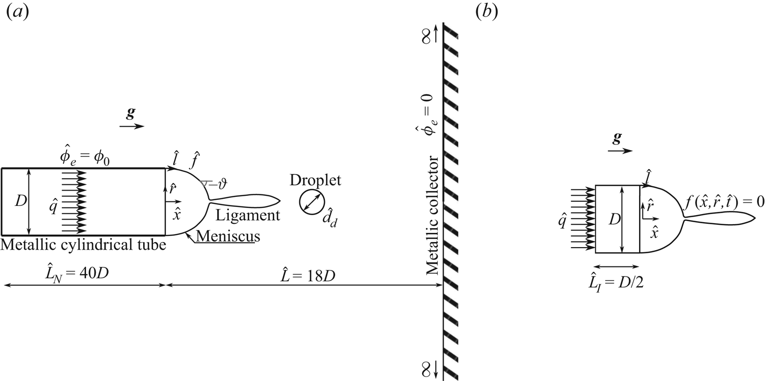
 $D$, and infinitely thin wall, discharging into the space between the tube and a very large, flat collector electrode normal to the tube; see the sketch in figure 1(
 $a$). The distance
 $\hat {L}$ between the tube and the collector electrode is large compared with the diameter of the tube,
 $\hat {L}/D \gg 1$. An electric field,
 $\hat {\boldsymbol {E}}$, is created between the tube and the collector electrode when a voltage difference
 $\phi _0$ is applied between both. Cylindrical coordinates
 $\hat {x}$ and
 $\hat {r}$ are used, which are distances along and normal to the symmetry axis, with
 $\hat {x}=0$ at the end of the tube.
Model sketch to solve the electric potential ( $a$) and the velocity potential (
 $b$).

2.1. Model formulation
The surface of the liquid is considered electrically equipotential at the voltage of the tube, and the movement of the meniscus perturbs the electric field in the vicinity of the tube's tip. Leaving out the charge of the droplets emitted by the meniscus, the electric potential outside the liquid,  $\hat {\phi }_e$, satisfies the Laplace equation, which is solved outside the liquid in the region sketched in figure 1(
 $a$) with the boundary conditions
 $\hat {\phi }_e=0$ at the collector electrode
 $\hat {x}=\hat {L}$ and infinitely far from the tube and the liquid, and
 $\hat {\phi }_e=\phi _0$ at the tube and the meniscus.
The flow of the liquid is considered irrotational, and the velocity potential,  $\hat {\phi }$ such that
 $\hat {\boldsymbol {v}}=\boldsymbol {\nabla }\hat {\phi }$, obeys the Laplace equation in the liquid, both in the meniscus and inside the tube, as sketched in figure 1(
 $b$). We consider homogeneous Neumann conditions at the wall of the tube
 $-\hat {L}_{I}<\hat {x}<0$,
 $\hat {r}=D/2$, and
 $\partial \hat {\phi }/\partial \hat {x}=4\hat {q}/({\rm \pi} D^2)$ at an inlet section
 $\hat {x}=-\hat {L}_{I}$,
 $\hat {r}< D/2$. On the surface of the liquid, defined by the unknown function
 $f(\hat {x},\hat {r},\hat {t})=0$, with
 $f<0$ in the liquid, the kinematic condition,
 $Df/D\hat {t}=0$, and the dynamic condition,
 $\partial _{\hat {t}}\hat {\phi }+\hat {p}/\rho +|\boldsymbol {\nabla }\hat {\phi }|^2/2-g\hat {x}=0$ (which holds everywhere in the liquid), must be satisfied, where
 $\hat {p}$ is the pressure of the liquid referred to the outer medium,
 $g$ is the acceleration of the gravity and
 $D/D\hat {t}=\partial _{\hat {t}}+\hat {\boldsymbol {v}}\boldsymbol {\cdot }\boldsymbol {\nabla }$ (Landau & Lifshitz Reference Landau and Lifshitz1987).
At the surface of the liquid, the pressure  $\hat {p}$ can be written from a balance of normal stresses at the meniscus surface as
 $\hat {p}=\gamma \hat {\kappa } -\epsilon _0 \hat {E}^2 /2$, where
 $\hat {\kappa }$ is twice the mean curvature of the surface, so that
 $\gamma \hat {\kappa }$ is the capillary pressure,
 $\epsilon _0$ is the electric permittivity of vacuum and
 $\epsilon _0 \hat {E}^2/2$ is the electric stress, which is normal to the surface and is obtained from the Maxwell stress tensor (Landau & Lifshitz Reference Landau and Lifshitz1984). The curvature of the meniscus is calculated in terms of the arclength,
 $\hat {l}= \int _0^{\hat {l}}\sqrt {1+(\mathrm {d}{\hat {r}}/\mathrm {d}{\hat {x}})^2}\,\mathrm {d}{\hat {x}}$ with
 $\hat {l}=0$ at the contact line of the meniscus and the tube, and the slope angle,
 $\vartheta$, with
 $\tan {\vartheta }=\mathrm {d}{\hat {r}}/\mathrm {d}{\hat {x}}$:
 $\hat {\kappa }=-\mathrm {d}{\vartheta }/\mathrm {d}{\hat {l}}+\cos (\vartheta )/\hat {r}$. For a liquid of infinite conductivity, the electric field is normal to its surface,
 $\hat {\boldsymbol {E}}=\hat {E}\boldsymbol {n}$, where
 $\boldsymbol {n}=\boldsymbol {\nabla } f/|\boldsymbol {\nabla } f|$ is the unit normal to the meniscus surface pointing away from the liquid.
Summarizing, the mathematical formulation of the model problem is
 \begin{gather} \nabla^2 \hat{\phi}_e=0 \quad \text{outside the liquid}, \text{ with }\hat{\boldsymbol{E}}={-}\boldsymbol{\nabla} \hat{\phi}_e, \end{gather}
 \begin{gather} \nabla^2 \hat{\phi}=0 , \quad \frac{\partial \hat{\phi}}{\partial \hat{t}} + \frac{1}{2} \left| {\boldsymbol{\nabla} \hat{\phi} } \right|^2 + \frac{\hat{p}}{\rho} - g \hat{x} = 0 \quad \text{in the liquid},\text{ with }\hat{\boldsymbol{v}}=\boldsymbol{\nabla} \hat{\phi},\end{gather}
 \begin{gather} \left. \begin{gathered} \hat{\phi}_e= \phi_0, \\ \frac{\partial f}{\partial \hat{t}} + \frac{\partial \hat{\phi}}{\partial \hat{x}} \frac{\partial f}{\partial \hat{x}} + \frac{\partial \hat{\phi}}{\partial \hat{r}} \frac{\partial f}{\partial \hat{r}} = 0, \\ \frac{\partial \hat{\phi}}{\partial \hat{t}} + \frac{1}{2} \left| {\boldsymbol{\nabla} \hat{\phi}} \right|^2 - g \hat{x} = \frac{1}{\rho} \left( {\frac{1}{2} \epsilon_0 \hat{E}^2 - \gamma \hat{\kappa} } \right), \end{gathered}\right\} \quad \text{at the surface of the liquid,} \end{gather}
 \begin{gather} \hat{\phi}_e=0, \quad \text{at the collector electrode and far from the liquid }(\hat{r} \rightarrow \infty), \end{gather}
 \begin{gather} \hat{\phi}_e = \phi_0 , \quad \text{at the wall and the far base of the tube}, \end{gather}
 \begin{gather} \frac{\partial \hat{\phi}}{\partial \hat{r}} = 0, \quad \text{at the surface of the tube between }\hat{x}={-}\hat{L}_{I}\text{ and }\hat{x}=0, \end{gather}
 \begin{gather} \frac{\partial \hat{\phi}}{\partial \hat{x}} = \frac{4 \hat{q}}{{\rm \pi} D^2}, \quad \text{at the inlet section }\hat{x}={-}\hat{L}_{I},\ \hat{r}< D/2. \end{gather}
A time periodic solution of this problem is sought by starting at an arbitrary initial state (see below) and letting the system evolve in time through a number of cycles of elongation, droplet emission and retraction of the meniscus.
The treatment of droplet emission from the tip of the meniscus requires additional approximations. A droplet is assumed to detach from the meniscus when the local radius of the surface of the liquid ( $\hat {h}(\hat {x}, \hat {t})$ say) develops a minimum smaller than a selected threshold,
 $\min _{\hat {x}} \hat {h} < \hat {r}_m$. Whenever this happens, the tip of the meniscus is cut and rounded at the position of minimum
 $\hat {h}$, assigning the lost volume to a droplet emitted from the tip. However, the presence of the droplet is not subsequently accounted for in the computations.
Two types of droplets are emitted from a real meniscus in the microdripping mode. On the one hand, the meniscus develops an apparent conical tip during part of the oscillation cycle, whose apparent vertex emits a spray of very small droplets, of size comparable to the characteristic size  $r_e$ of the region where the surface of the liquid is not equipotential (see introduction and § 2.3 below). On the other hand, the meniscus develops a ligament during its elongation, whose periodic detachment originates one or a few larger droplets per cycle. Apparent conical tip means here that the tip resembles a cone at the scale of the whole meniscus. However, the curvature of the surface at the tip is finite except at the instants when pinch-off occurs, though it may be very large. The tip is a regular point, and the solutions of (2.1) and (2.2) are regular there. The normal to the surface is well defined at the tip, and no special treatment of this point is needed. The fact that
 $\partial \hat {h}/\partial \hat {x}$ tends to infinity at the tip is of no consequence because the contour of the meniscus is described parametrically in terms of the arclength
 $\hat {l}$.
The value of  $r_e$ is much smaller than the size of the meniscus, and the equipotential surface model cannot describe the flow in the small droplets emission region. The threshold value
 $\hat {r}_m$ is always much larger than
 $r_e$, so that the small droplets yielded by the model are far larger and less numerous than in reality, its size depending on the artificial threshold
 $\hat {r}_m$. The large droplets, on the contrary, are well resolved by the model. Despite this limitation, forced upon us by the multiscale character of the problem, the model still gives reasonable results for large-scale features such as the oscillation frequency and the size and charge of the large droplets, in ample ranges of the control parameters. The reason probably is that the fast dynamics of the ill resolved small droplets emission region is dictated by the slow dynamics of the meniscus bulk.
2.2. Non-dimensionalization
The problem is made non-dimensional using as scale factors the tube's diameter,  $D$, the capillary time,
 $t_c=(\rho D^3/\gamma )^{1/2}$, the surface tension
 $\gamma$ and the applied voltage,
 $\phi _0$. Velocities are scaled with the capillary velocity
 $v_c=[\gamma /(\rho D)]^{1/2}$, the flow rate with
 $q_c=(\gamma D^3/\rho )^{1/2}$, the velocity potential with
 $\phi _c=v_c D$ and the electric potential and the electric field with
 $\phi _0$ and
 $E_c=\phi _0/D$. For convenience, the electric charge and the electric current are scaled with
 $(\epsilon _0 \gamma D^3)^{1/2}$ and
 $(\epsilon _0 \gamma ^2/\rho )^{1/2}$, respectively.
For a given set-up (i.e.  $L=\hat {L}/D$ fixed, as well as
 $L_{I}=\hat {L}_{I}/D$ and
 $L_{N}=\hat {L}_{N}/D$, though the last two parameters have little effect on the solution), the problem depends on three dimensionless parameters, which are a electric Bond number,
 ${B_{E}}$, a Bond number,
 ${B}$, and a dimensionless flow rate,
 $q$, or a dimensionless injection velocity,
 $v_o$ at
 $x=-L_{I}, r<1/2$. These parameters are
 $$\begin{gather} {B_{E}}=\dfrac{\epsilon_0 E_c^2 D}{\gamma}, \end{gather}$$
 $$\begin{gather}{B}=\dfrac{\rho g D^2}{\gamma}, \end{gather}$$
 $$\begin{gather}q=\frac{\rm \pi}{4} v_o= \dfrac{\rho^{1/2} \hat{q}}{\gamma^{1/2} D^{3/2}}. \end{gather}$$
In what follows, dimensionless variables are denoted with the same symbols used in (2.1)–(2.7) for their dimensional counterparts, with the hat removed. The dimensionless equations and boundary conditions coincide with (2.1)–(2.7) except that  $D$,
 $\rho$,
 $\gamma$ and
 $\phi _0$ are replaced by unity, and
 $\epsilon _0$ and
 $g$ are replaced by
 ${B_{E}}$ and
 ${B}$.
2.3. Charge transport in the liquid
Transport of charged species in the liquid occurs due to migration, convection and diffusion when a voltage is applied between the metallic tube and the plate. In the simplest case, this leads to a flux  $\hat {\boldsymbol {j}}_i=\nu _i \hat {n}_i \hat {\boldsymbol {E}} + \hat {n}_i \hat {\boldsymbol {v}} - D_i \boldsymbol {\nabla } \hat {n}_i$ for species
 $i$, where
 $\nu _i$ and
 $D_i$ are the mobility and diffusion coefficient of this species,
 $\hat {n}_i$ is its number density and
 $\hat {\boldsymbol {v}}$ is the velocity of the liquid. Conservation equations for fully dissociated species are
 $\partial _{\hat {t}} \hat {n}_i + \boldsymbol {\nabla } \boldsymbol {\cdot } \hat {\boldsymbol {j}}_i = 0$, while charge conservation requires
 $\partial _{\hat {t}} \hat {\rho }_e + \boldsymbol {\nabla } \boldsymbol {\cdot } \hat {\boldsymbol {J}} = 0$. Here
 $\hat {\rho }_e=\sum _i {\mathcal {C}}_i \hat {n}_i$ and
 $\hat {\boldsymbol {J}} = \sum _i {\mathcal {C}}_i \hat {\boldsymbol {j}}_i$ are the charge and electric current densities, with
 ${\mathcal {C}}_i$ the charge of species
 $i$. Since
 $\boldsymbol {\nabla } \boldsymbol {\cdot } \hat {\boldsymbol {E}} = \hat {\rho }_e/\epsilon _0 \epsilon$ and
 $\boldsymbol {\nabla } \boldsymbol {\cdot } \hat {\boldsymbol {v}} = 0$, where
 $\epsilon$ is the dielectric constant of the liquid, the condition of charge conservation can be written as
 $D\hat {\rho }_e/D\hat {t} =-K \hat {\rho }_e/\epsilon _0 \epsilon - \hat {\boldsymbol {E}} \boldsymbol {\cdot } \boldsymbol {\nabla } K + \boldsymbol {\nabla } \boldsymbol {\cdot } ( {\sum {\mathcal {C}}_i D_i \boldsymbol {\nabla } \hat {n}_i} )$, where
 $K=\sum _i {\mathcal {C}}_i \nu _i \hat {n}_i$ would be the electrical conductivity of the liquid in cases when Ohm's law can be used. The first term on the right-hand side of this equation implies that
 $\hat {\rho }_e$ tends to zero, establishing quasi-neutrality in the liquid, in a time of the order of the electric relaxation time
 $t_e=\epsilon _0 \epsilon /K$. As was mentioned before, this time is short compared with the characteristic time of the meniscus,
 $t_c$, implying that
 $\hat {\rho }_e \approx 0$ in the bulk of the liquid, even in cases when electric charges are injected upstream of the meniscus by means of an electrode immersed in the liquid. Quasi-neutrality also holds in the small region of characteristic size
 $r_e$ that may exist around the tip of the meniscus. The residence time of the liquid in this region is not large compared with
 $t_e$, but the liquid enters this region already with
 $\hat {\rho }_e \approx 0$.
Diffusion matters in a thin non-neutral layer by the surface of the liquid where electric charge accumulates under the action of the electric field due to the applied voltage. The field induced by this charge in the bulk of the liquid opposes the component normal to the surface of the field due to the applied voltage. The time it takes for the non-neutral layer to attain a steady state and reduce to zero the component of the electric field normal to the surface in the bulk of the liquid is  $t_e$. This can be seen from the balance of accumulation and migration in the conservation equations for the charged species during the charging of the layer. Calling
 $\hat {\delta }$ the characteristic thickness of the layer,
 $\hat {t}_{ch}$ the characteristic time of charging,
 $\hat {E}_l$ the electric field at the liquid side of the surface, and
 ${\mathcal {C}}_c$,
 $\nu _c$ and
 $\hat {n}_c$ the characteristic charge, mobility and number density of the relevant species, so that
 ${\mathcal {C}}_c \nu _c \hat {n}_c \sim K$, this balance reads
 $\hat {n}_c/\hat {t}_{ch} \sim \nu _c \hat {n}_c \hat {E}_l/\hat {\delta } \sim \nu _c {\mathcal {C}}_c \hat {n}_c^2/\epsilon _0 \epsilon$, where the last estimation comes from the Poisson equation in the layer:
 $\hat {E}_l/\hat {\delta } \sim {\mathcal {C}}_c \hat {n}_c/\epsilon _0 \epsilon$. Hence
 $\hat {t}_{ch} \sim t_e$ and the liquid acts as a perfect conductor when this time is short compared with the characteristic time of the flow.
This condition is not always satisfied uniformly. It fails in the small region around the tip of the meniscus mentioned above, in the part of the oscillation cycle when a spray of very fine droplets is emitted. The residence time of the liquid in this region is of the order of  $t_e$, as was already mentioned, and the electric field due to the applied voltage gets into the liquid. This small relaxation region will not be analysed here.
2.4. Inviscid liquid assumption
The assumption of inviscid liquid is reasonable for water solutions such as the liquid used in the experiments of Hijano et al. (Reference Hijano, Loscertales, Ibáñez and Higuera2015), for which the velocity is of the order of the capillary velocity  $v_c=[\gamma /(\rho D)]^{1/2}$ and the Ohnesorge number,
 ${Oh}=\mu /\sqrt {\rho \gamma D}$, is of the order of
 $10^{-2}$. So viscous effects are considerably less important than the effects of inertia or capillary forces. Gravitational forces are also small,
 ${B}\sim 10^{-2}$, but they are retained in the analysis.
3. Numerical procedure and results
3.1. Numerical method
The Laplace equations for the velocity and electric potentials,  $\phi$ and
 $\phi _e$, are solved by boundary element methods (BEM). Each of these equations is rewritten as an integral equation on the boundary of the region where it has to be solved, and the surface integrals reduce to line integrals on a meridional section of the boundary taking advantage of the axisymmetry of the problem; see, for example, Pozrikidis (Reference Pozrikidis2002). At a given time, for a given position of the liquid surface, the equation for the velocity potential is
 $$\begin{align} \phi(x_0,r_0) &={-}2\int_{C_1}{G_1(x,r,x_0,r_0) v_n(x,r) r \, \mathrm{d}{l}}\nonumber\\ &\quad + 2\int_{C_1}^{PV}{G_{1n}(x,r,x_0,r_0) \phi(x,r) r \, \mathrm{d}{l}} , \end{align}$$
where the contour  $C_1$ is made of meridional sections of the surface of the liquid,
 $f(x,r,t)=0$ at the instant considered, the wall of the tube between
 $x=-L_{I}$ and
 $x=0$, and the inlet section, (
 $x=-L_{I}$,
 $r<1/2$);
 $v_n=\boldsymbol {n}_i \boldsymbol {\cdot } \boldsymbol {\nabla } \phi$ with the unit normal vector
 $\boldsymbol {n}_i$ pointing inward (into the liquid domain);
 $l$ denotes the arclength along the contour,
 $x(l)$ and
 $r(l)$ is a generic point on
 $C_1$, parameterized with the arclength, and
 $x_0=x(l_0)$,
 $r_0=r(l_0)$ is a fixed point on
 $C_1$; and
 $G_1$ and
 $G_{1n}=\partial _{n_i} G_1$ are the Green function for an axisymmetric ring of sources and its normal derivative, see Pozrikidis (Reference Pozrikidis2002). The
 $PV$ in the second integral stands for Cauchy's principal value. The contour
 $C_1$ is discretized using
 $N_1$ points (of which
 $N$ are on the surface of the meniscus, equispaced in the arclength), linear interpolation is used for
 $\phi$ and
 $v_n$ in each element, and the integrals are evaluated using four points Gaussian integration. The solution of the discretized form of (3.1) determines
 $v_n$ at the points on the liquid surface, and
 $\phi$ at the points on the tube wall and the inlet section, in terms of
 $\phi$ at the points on the liquid surface.
Similarly, for the electric potential  $\phi _e$,
 $$\begin{align}
\phi_e(x_0,r_0) &= 2 \int_{C_2}{G_2(x,r,x_0,r_0) E(x,r) r \,
\mathrm{d}{l}} \nonumber\\ &\quad + 2
\int_{C_2}^{PV}{G_{2n}(x,r,x_0,r_0) \phi_e(x,r) r \,
\mathrm{d}{l}} ,
\end{align}$$
where  $E=\boldsymbol {n}_i \boldsymbol {\cdot } \boldsymbol {\nabla } \phi _e$ and
 $G_{2n}$ is the normal derivative of
 $G_2$, with the unit normal vector
 $\boldsymbol {n}_i$ now pointing outward from the meniscus and the tube. In principle,
 $C_2$ is made of meridional sections of the surface of the liquid, the surfaces of the tube and the section (
 $x=-L_{N}$,
 $r<1/2$), and the surface of the collector, and closes at infinity. However, the collector is replaced by the images of the other surfaces by using for
 $G_2$ the potential of an axisymmetric ring of sources and its image in the collector, so that
 $G_2=0$ at points
 $(x_0, r_0)$ on the collector. In addition, since the net charge of the ring of sources plus its image is zero, the electric field decreases faster than the inverse of the square of the distance to the meniscus and the tube, and the contributions to the integrals of the segment of
 $C_2$ at infinity are null. Thus, only the contours of the meniscus, the tube and the section (
 $x=-L_{N}$,
 $r<1/2$) need be considered in
 $C_2$, and the electric potential
 $\phi _e=1$ in the second integral of (3.2) on these contours. This
 $C_2$ is discretized using
 $N_2$ points (
 $N$ of them on the meniscus). The same linear interpolation and Gaussian integration mentioned above are used for (3.2). The solution of the discretized form of (3.2) determines
 $E$ at all the points on
 $C_2$. The dimensionless length of the tube and its distance to the collector electrode are taken to be
 $L_{N}=40$ and
 $L=18$, which correspond to the values
 $\hat {L}_{N}=20$ mm and
 $\hat {L}=9$ mm in the experiments of Hijano et al. (Reference Hijano, Loscertales, Ibáñez and Higuera2015). To save computer time, the dimensionless distance to the inlet section is taken to be
 $L_{I}=0.5$. Numerical tests show that the solution does not change when this value is increased.
The Green functions and their derivatives are written in terms of complete elliptic integrals of the first and second kind,  $F(k)$ and
 $E(k)$, with
 $k^2=4 r r_0/[(x-x_0)^2+(r+r_0)^2]$. Both elliptic integrals are approximated as
 $F(k) \approx a_1-a_2\log (1-k^2)$ and
 $E(k) \approx a_3-a_4\log (1-k^2)$, respectively, with
 $a_i=\sum _{j=0}^{j=4} b_{ij}(1-k^2)^j$ and
 $b_{ij}$ given by Pozrikidis (Reference Pozrikidis2002). Points (
 $x_0$,
 $r_0$) are located at the centres of the linear elements.
Once  $v_n$ and
 $E$ are computed at the surface of the liquid (in terms of the unknown
 $\phi$), the following differential equations can be set up for the time evolution of material particles coinciding with the discretization points of the surface and the values of the velocity potential at these material particles:
 $$\begin{gather} \dfrac{\textrm{D} x}{\textrm{D} t}=v_x , \end{gather}$$
 $$\begin{gather}\dfrac{\textrm{D} r}{\textrm{D} t}=v_r , \end{gather}$$
 $$\begin{gather}\dfrac{\textrm{D}\phi}{\textrm{D} t}=\dfrac{1}{2} \left( {v_n^2 + v_l^2} \right) + \dfrac{1}{2} {B_{E}} E^2 - \kappa + Bx , \end{gather}$$
where the derivatives on the left-hand sides are material derivatives,  $\textrm {D} (\cdot )/\textrm {D} t = \partial _t (\cdot ) + \boldsymbol {v} \boldsymbol {\cdot } \boldsymbol {\nabla } (\boldsymbol {\cdot })$, with
 $\boldsymbol {v} = (v_x, v_r)$,
 $v_x=v_l \cos \vartheta - v_n \sin \vartheta$,
 $v_r=v_l \sin \vartheta + v_n \cos \vartheta$. Here
 $v_l=\partial _l \phi$ is obtained by numerically differentiating the discretized
 $\phi$ with respect to the arclength. These equations (three per discretization point on the liquid surface) are solved using the adaptive Runge–Kutta–Fehlberg method of fourth order (Mathews & Fink Reference Mathews and Fink1999). The discretization points are changed at each time step to keep them equidistributed on the surface, and
 $\phi$ is interpolated to the new discretization points. We arbitrarily impose
 $\phi =0$ at
 $x=0$,
 $r=1/2$ at each time step, a renormalization allowed by boundary conditions (2.3) and (2.6)–(2.7).
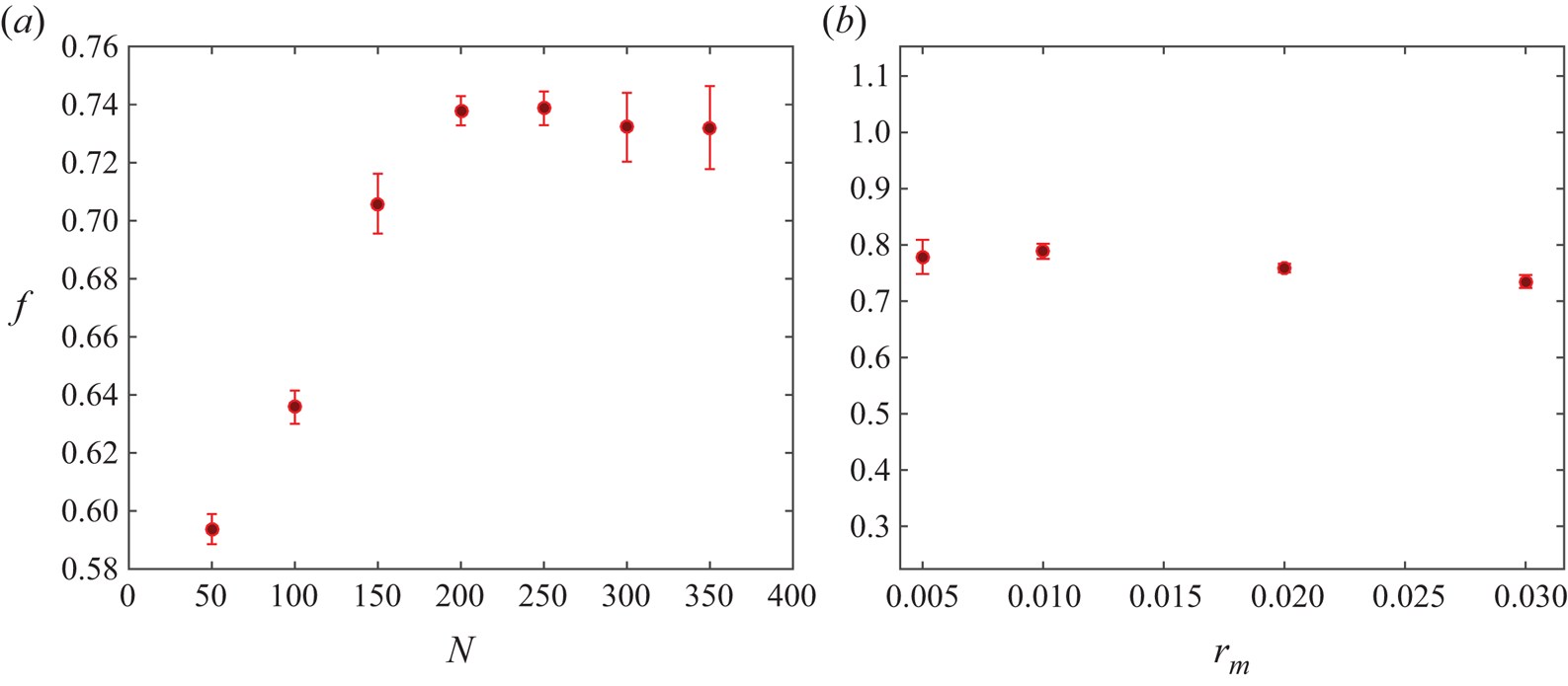
Numerical tests have been used to analyse the effects of the threshold  $r_m$ and the number of nodes on the meniscus,
 $N$. The results show that the computed number and size of small droplets emitted from the tip during an oscillation cycle depend on
 $r_m$. However, large-scale magnitudes such as the meniscus oscillation frequency and the size of the large droplet emitted when the ligament detaches are fairly independent of these numerical parameters when
 $N$ is larger than approximately 150, provided
 $N$ is increased when
 $r_m$ is decreased, in such a way that the mean spacing of the nodes is not large compared with
 $r_m$. Very small values of
 $r_m$ without a sufficiently large
 $N$ may lead to spurious solutions with artificially long ligaments, because the condition of detachment from the tip,
 $\min _x h < r_m$, may not be satisfied for small droplets. On the basis of these tests, we have chosen
 $r_m=10^{-2}$ and
 $N=200$, while the numbers of nodes on the solid surface of the tube used to discretize (3.1) and (3.2) are
 $N_1-N=60$ and
 $N_2-N=260$, respectively (non-equispaced). Figure 2(
 $a$) shows the oscillation frequency of the meniscus (
 $f$) when a periodic regime is reached versus the number of equispaced points on the meniscus (
 $N$) for
 $r_m=10^{-2}$, and figure 2(
 $b$) shows
 $f$ versus
 $r_m$ when
 $r_m$ is of the order of the distance between two consecutive points on the meniscus.
( $a$) Dimensionless oscillation frequency of the meniscus,
 $f$, versus the number of equispaced points on the meniscus,
 $N$, with
 $r_m=10^{-2}$; (
 $b$)
 $f$ versus
 $r_m$, where
 $N$ is increased when
 $r_m$ decreases, to maintain of order one the relation between
 $r_m$ and the distance between two consecutive points on the meniscus. Results are shown for
 $q=4.56\times 10^{-2}$,
 ${B_{E}}=3.72$ and
 ${B}=6.3 \times 10^{-2}$.

3.2. Validation of the numerical code
The numerical code has been validated by computing the oscillation of an electrified free inviscid drop of a perfectly conducting liquid in a vacuum. In a classical work, Rayleigh (Reference Rayleigh1882) solved the linearized problem for small amplitude oscillations. Scaling distances with the radius  $R$ of the equilibrium drop and times with
 $(\rho R^3/\gamma )^{1/2}$, where
 $\rho$ and
 $\gamma$ are the density and surface tension of the liquid, and using spherical coordinates with origin at the centre of the drop (see inset of figure 3
 $b$), the eigensolutions of the linear problem have surface deformations
 $R_p(\theta ,t)-1=\delta \, P_n(\cos \theta ) \textrm {e}^{2{\rm \pi} \textrm {i} f_n t}$ and oscillation frequencies
 $2 {\rm \pi}f_n = [n (n-1) (n+2) - {\tilde {B}_{E}} n (n-1)]^{1/2}$, with
 $n=2, 3, \dots$. Here
 $P_n$ are Legendre polynomials and
 ${\tilde {B}_{E}}=Q^2/(16 {\rm \pi}^2 \epsilon _0 \gamma R^3)$, where
 $Q$ is the electric charge of the drop, which becomes unstable when
 ${\tilde {B}_{E}}>4$.
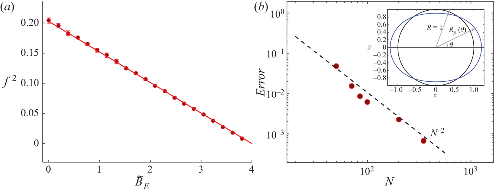
( $a$) Square of the dimensionless free oscillation frequency,
 $f^2$, versus
 ${\tilde {B}_{E}}$ for
 $N=100$ (circles) compared with the frequency of Rayleigh's linear theory for
 $n=2$ (solid line). (
 $b$) Numerical error of the method versus number of equispaced points on the drop surface for
 ${\tilde {B}_{E}}=2.6667$ (circles). A sketch of the droplet deformation is included (for visualization purposes, the amplitude of the deformation in the sketch is larger than in the computations).

For the validation, the surface of the drop is discretized with  $N$ equispaced points and the full discrete problem (without linearization) is solved with an initial deformation of the surface corresponding to the first eigenmode of the linear problem (
 $n=2$) and
 $\delta =10^{-2}$. Figure 3(
 $a$) compares the oscillation frequency computed as a function of
 ${\tilde {B}_{E}}$ using
 $N=100$ points (circles) with the frequency of the linear oscillation (solid curve).
The order of the method is determined by computing, for  ${\tilde {B}_{E}}=2.6667$ and various values of
 $N$, the difference between the norm of the surface deformation and its value for
 $N=500$, which is taken to be close to the exact solution. The error is defined as
 \begin{equation} \text{error} = \frac{1}{2 \delta} \overline{ \left|\left[ {\int_{{-}1}^1 {(R_{pN} - 1)^2 \, \mathrm{d}{(\cos \theta)} } }\right]^{1/2} -\left[ {\int_{{-}1}^1 {(R_{p500} - 1)^2 \, \mathrm{d}{(\cos \theta)} } }\right]^{1/2}\right| } , \end{equation}
where  $R_{pN}-1$ is the deformation of the drop surface discretized with
 $N$ points and the overbar denotes averaging over a time interval spanning various oscillation cycles. This error is shown in figure 3(
 $b$) as a function of
 $N$. Owing to the weak nonlinearity of the problem, the solution computed with the initial condition mentioned above is not strictly periodic, which may be the cause of the small irregularity of the data points in the figure.
The attenuation of the surface oscillation is determined by fitting an exponential to the envelope of the oscillatory deformation. Values of the decaying rate, which is a numerical artefact, are of the order of the error displayed in figure 3( $b$).
3.3. Numerical results
The initial meniscus shape is a hemisphere. For given values of the flow rate,  $q$, electric Bond number,
 ${B_{E}}$, and Bond number,
 ${B}$, the simulation is run in time until a periodic oscillation of the meniscus is obtained.
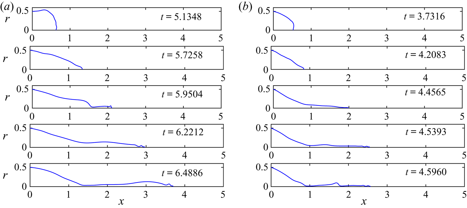
Figure 4 shows sequences of five snapshots of the dimensionless meniscus contour, from its most retracted position to its most elongated one (prior to pinch-off), for  ${B_{E}}=3.72$ and
 ${B}=6.3 \times 10^{-2}$, with
 $q=5.79 \times 10^{-2}$ in the sequence in panel
 $(a)$ and
 $q=6.82 \times 10^{-3}$ in the sequence in panel
 $(b)$. The meniscus begins to elongate from its retracted position until it adopts a quasi-conical shape (second snapshot from the top in panels
 $(a)$ and
 $(b)$), after which small droplets begin to be ejected from the meniscus tip. As time advances, the meniscus develops a ligament whose tip keeps on emitting bursts of small droplets (snapshots 3 and 4 in both cases). The ligament is stretched and finally detaches from the meniscus (the last snapshot of each panel sequence shows the meniscus immediately before detachment), generating a droplet much larger than those previously emitted during the cycle. After the detachment, the meniscus recedes violently (not shown) and the same process starts again periodically. Figure 4 also shows the strong influence of the flow rate
 $q$ on the meniscus mean volume, the length and width of the ligament, and the volume of the droplet emitted upon its detachment. The main features are similar to those observed in the experiments, except that the droplets emitted from the tip before the ligament detaches are far larger and less numerous than in the experiments. These droplets should make the electrospray at the conical tip, but in reality they are too small to be seen in the video images. The size of the small droplets in the simulations is related to the artificial threshold
 $r_m$ introduced above.
Dimensionless meniscus profile at different stages during its oscillation for two different flow rates,  $q=5.79\times 10^{-2}$ (
 $a$) and
 $q=6.82\times 10^{-3}$ (
 $b$), with
 ${B_{E}}=3.72$ and
 ${B}=6.3 \times 10^{-2}$. The dimensionless time is specified in each panel.

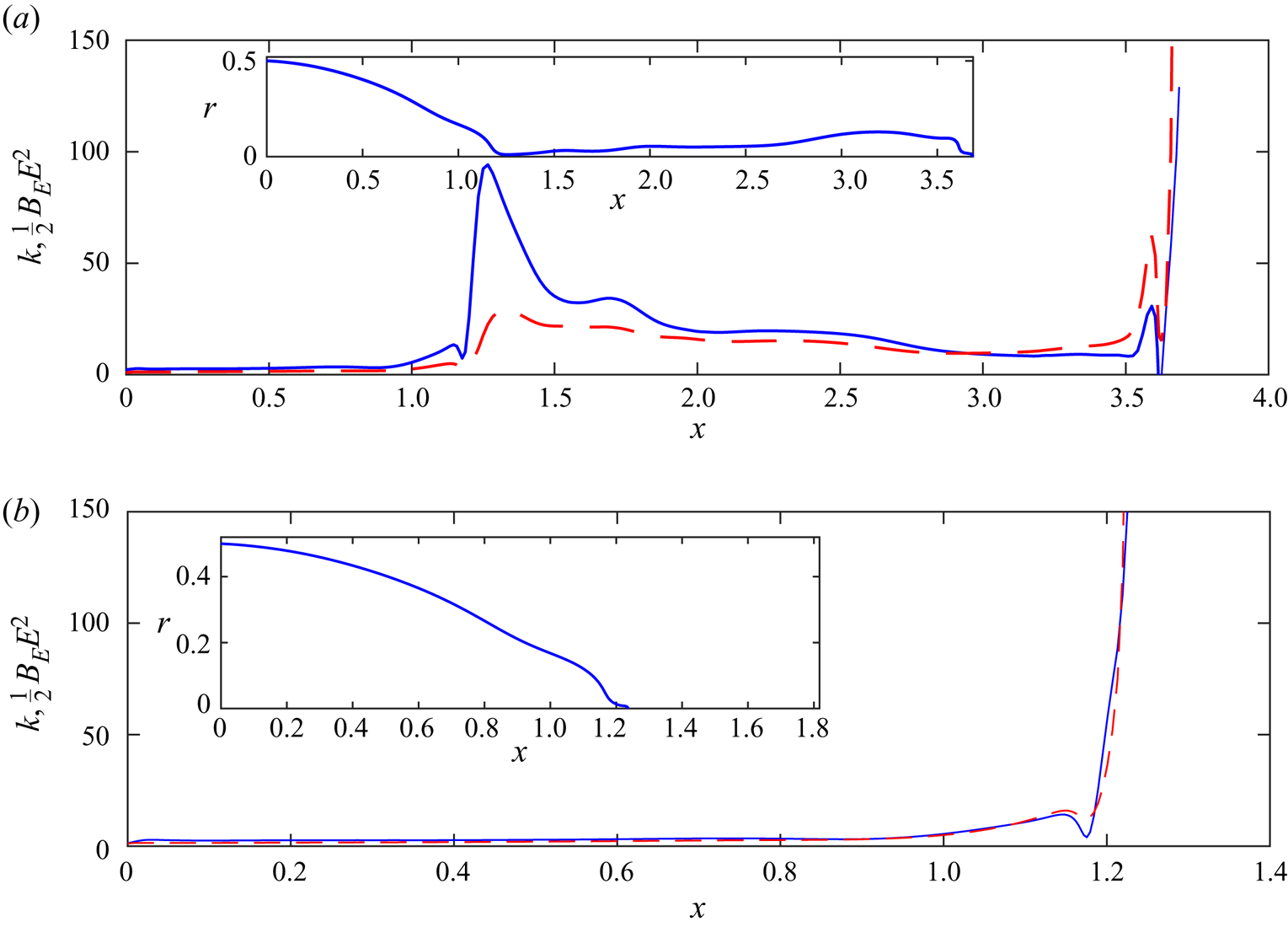
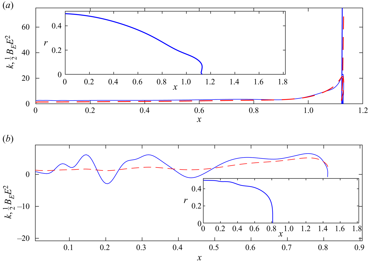
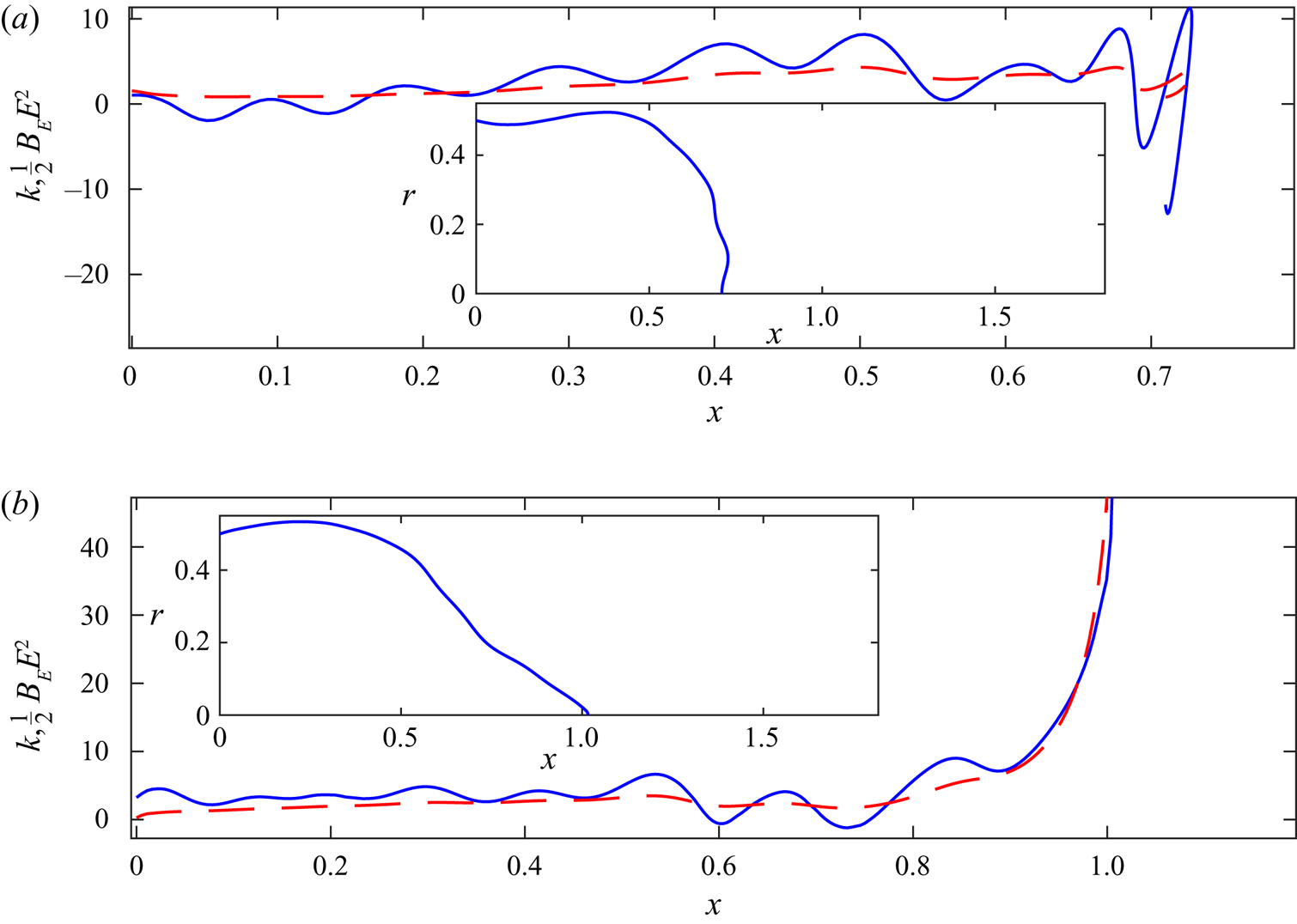
The simulations allow measuring the importance of the capillary and electric stresses on each point of the meniscus surface at any stage of its oscillation, and so checking if the assumptions made in Hijano et al. (Reference Hijano, Loscertales, Ibáñez and Higuera2015) are appropriate. Figures 5–7 show the dimensionless capillary and electric stresses on the meniscus,  $\kappa$ and
 ${B_{E}} E^2 /2$, respectively, versus the dimensionless axial position,
 $x$, at various stages of the meniscus oscillation.
Capillary stress (solid) and electric stress (dashed) on the meniscus surface just before ( $a$) and after (
 $b$) the ligament detachment. Inset: dimensionless meniscus shape. Results are shown for
 $q=5.79\times 10^{-2}$,
 ${B_{E}}=3.72$ and
 ${B}=6.3\times 10^{-2}$.

Figure 5( $a$) shows a meniscus with an elongated ligament right before its detachment. The ligament is fully stretched and the neck where the capillary stresses are going to produce the pinch-off can be clearly observed. As assumed in Hijano et al. (Reference Hijano, Loscertales, Ibáñez and Higuera2015), the capillary and electric stresses nearly balance each other along the ligament, where they are almost constant, whereas the capillary stress dominates around the neck and the electric stress dominates around the tip. Right after the detachment, figure 5(
 $b$), the electric stress at the new formed tip is stronger than the capillary stress, leading to the ejection of more small droplets from the meniscus tip until the capillary stress takes over and the meniscus begins to recede violently with a velocity of the order of the capillary velocity. This feature is not observed in the experiments, where there are no emissions from the newly formed tip of the meniscus after the detachment of the ligament. The beginning of the recession period is shown in figure 6(
 $a$). As mentioned before, the capillary stress eventually becomes dominant at the tip leading to a retraction of the meniscus. Figure 6(
 $b$) shows an instant where the retraction velocity is of the order of the capillary velocity. Some capillary waves begin to form. After the retraction, the meniscus elongates again, figure 7(
 $a$), and a rounded tip is formed later on, figure 7(
 $b$), when the electric stress begins to take over around the tip. Capillary waves can be observed also at this stage. In subsequent times, small droplets will start being ejected from the tip and the ligament begins to form.
Capillary stress (solid) and electric stress (dashed) during the first stages of the retraction ( $a$) and during its violent retraction (
 $b$). Results are shown for
 $q=5.79 \times 10^{-2}$,
 ${B_{E}}=3.72$ and
 ${B}=6.3 \times 10^{-2}$.

Capillary stress (solid) and electric stress (dashed) when the meniscus starts to elongate after the retraction stage ( $a$) and when a pointed tip starts to form (
 $b$). Results are shown for
 $q=5.79 \times 10^{-2}$,
 ${B_{E}}=3.72$ and
 ${B}=6.3 \times 10^{-2}$.

The last stages of the process leading to pinch-off have been analysed in the absence of electric forces. For liquids of low viscosity, capillary forces and the inertia of the liquid dominate around the neck during much of its time evolution, with viscous forces coming in only at the last moment (see Day, Hinch & Lister (Reference Day, Hinch and Lister1998) and Leppinen & Lister (Reference Leppinen and Lister2003)). Even though the resolution of our computations is not enough to describe these stages in detail, figure 5( $a$) suggests that the analysis of the last cited references could hold also during the detachment of an electrified ligament. The first stages following pinch-off in the absence of electric forces have been analysed by Keller, King & Ting (Reference Keller, King and Ting1995) and Decent & King (Reference Decent and King2008), among others. However, the strong electric stress at the tip in figure 5(
 $b$) (which could be an artefact due to the numerical truncation of the surface) makes this analysis less certain for an electrified meniscus.
In the experiments, an ultrafine electrospray is also emitted during some phases of the duty cycle, in particular when a conical tip forms (Taylor cone). This is easily demonstrated by adding nanoparticles to the liquid: after operating the experiment for some minutes, one may observe on the collector a circular area of approximately one centimetre in diameter, in front of the needle, stained with nanoparticles even though no visible droplets landed in such region. The present model fails to simulate the electrohydrodynamics around the meniscus’ nose when a Taylor cone forms at the tip for the reason explained before. Namely, the assumption of perfect conductor liquid breaks down in a very small region around the tip where the residence time of the liquid is of the order of the electric relaxation time. In this region, the surface ceases to be equipotential, the electric field penetrates the liquid, and significant tangential electric stresses appear. In addition, the ultrafine electrospray generates a volumetric charge density around the meniscus tip, whose strength and distribution are unknown. Neither one of these effects are considered in the present model. As a result, the computations yield ligament shapes that may be different from those observed in the experiments. In the simulations, bursts of small droplets are emitted from the tip of the ligament as it stretches, the size of these droplets being dependent on the discretization used at the meniscus tip. Nevertheless, in situations where the conical tip is far from the oscillating meniscus, one would expect that the errors introduced by the limitations of the model on the dynamics of the meniscus will be small.
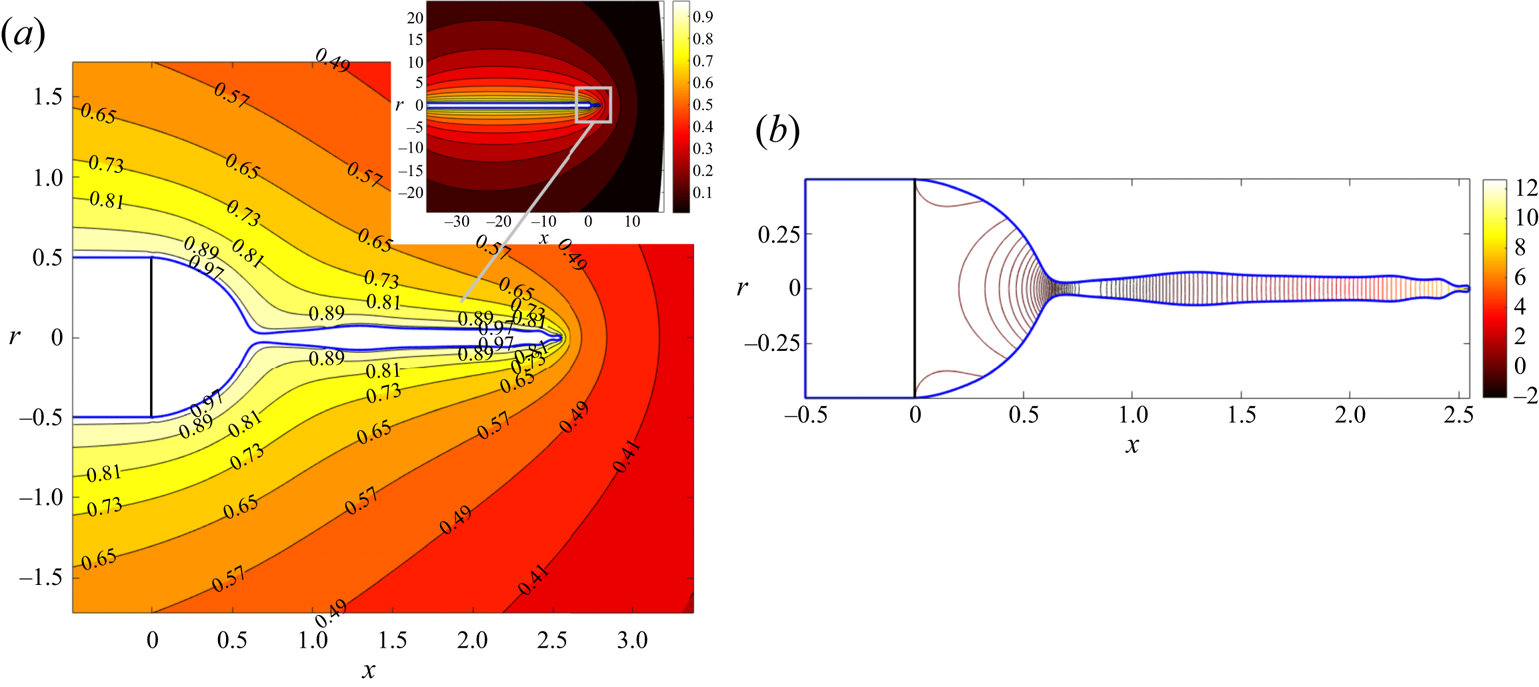
Sample contour maps of the electric potential outside the liquid and the velocity potential inside are shown in figure 8 shortly before the detachment of a ligament. The liquid flows from the neck, at approximately  $x=0.6$, into the ligament and the meniscus. In the ligament, the velocity increases toward the tip.
Contours of the electric potential,  $\phi _e$, around the meniscus (
 $a$) and of the velocity potential,
 $\phi$, in the liquid (
 $b$). Labels in panel (
 $a$) indicate the values of the electric potential. A solid line marks the end of the tube. Results are for
 $q=2.84 \times 10^{-2}$,
 ${B_{E}}=3.72$ and
 ${B}=6.3 \times 10^{-2}$, at a time shortly before the detachment of a ligament.

4. Comparison with experiments
Experiments were carried out by Hijano et al. (Reference Hijano, Loscertales, Ibáñez and Higuera2015) in which a constant flow rate of a mixture of water, ethanol and ethylene glycol conductivized with hydrochloric acid, with  $\rho =1065\ \textrm {kg}\,\textrm {m}^{-3}$,
 $\mu =2.3 \times 10^{-3}\ \textrm {Pa}\,\textrm {s}$,
 $\gamma =4.14 \times 10^{-2}\ \textrm {N}\,\textrm {m}^{-1}$ and
 $K=0.41\ \textrm {S}\,\textrm {m}^{-1}$, was injected through a vertical tube of outer diameter
 $D=500\ \mathrm {\mu }\textrm {m}$ set at a distance
 $\hat {L}=9$ mm from a horizontal collector. The values
 ${B_{E}}=3.72$ and
 ${B}=6.3 \times 10^{-2}$ were obtained when a voltage
 $\phi _0=2.95$ kV was applied between the tube and the collector.
4.1. Oscillations and droplet emission
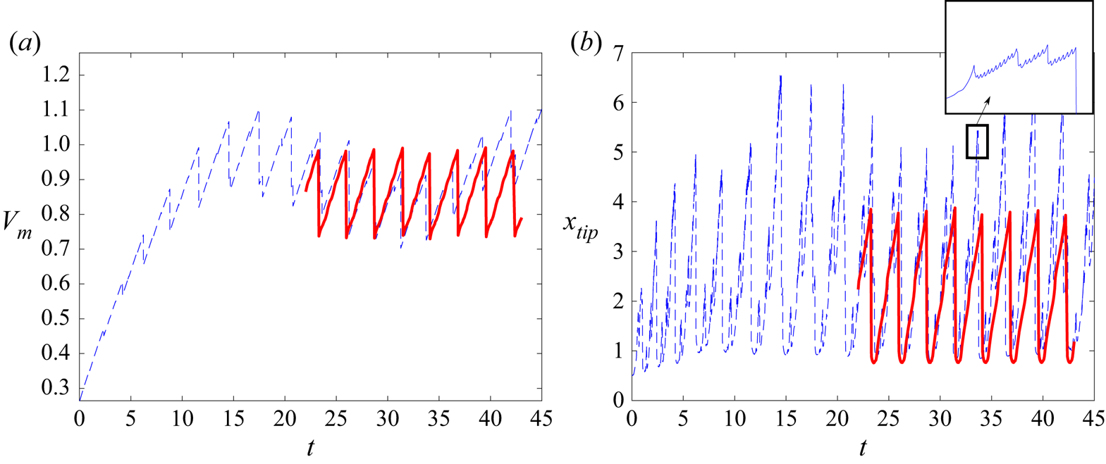
As mentioned before, the simulations start with an initial hemispherical meniscus that inflates while being fed at a constant flow rate. The electric stresses pull the meniscus, giving it an ellipsoidal-like shape as it continuously grows in volume. After some time, the electric stresses start tearing off a small mass of liquid from the meniscus tip while it keeps on growing and elongating, until a ligament forms and detaches. After this sequence repeats a certain number of times, a periodic state is reached in which the volume that enters the meniscus during a period of the oscillation equals the volume emitted from it in the form of droplets during that period. These processes can be observed in figure 9 for  $q=9.32\times 10^{-2}$,
 ${B_{E}}=3.72$ and
 ${B}=6.3\times 10^{-2}$. Dotted curves are numerical results while solid curves collect experimental results. Figure 9
 $(a)$ shows the dimensionless meniscus volume,
 $V_m$, versus the dimensionless time,
 $t$. It is interesting to note that the values of
 $V_m$ and the oscillation period are well captured by the simulations. However, it is also clear that the details of the emission of small droplets are not.
Temporal evolution of the meniscus volume ( $a$) and the axial position of the tip (
 $b$) for
 $q=9.32 \times 10^{-2}$,
 ${B_{E}}=3.72$ and
 ${B}=6.3 \times 10^{-2}$. Solid line for experiments and dashed line for simulations.

Figure 9( $b$) shows the dimensionless axial position of the meniscus tip,
 $x_{tip}$, versus the dimensionless time
 $t$. Whereas in the experiments there is apparently just one droplet emitted at the end of each oscillation, indicated by the steep fall of
 $x_{tip}$ (because the variation of
 $x_{tip}$ due to the emission of the tiny droplets making up the electrospray is too small to be seen), the simulations show two or three bursts of high-frequency emission of small droplets during the meniscus elongation, as indicated by the phases of highly oscillating
 $x_{tip}$ within each cycle of the meniscus oscillation, before a much larger droplet is eventually emitted at the end of the cycle. The inset of figure 9(
 $b$) is an enlargement of one of these high-frequency bursts.
A more detailed comparison between the experimental and numerical values of  $x_{tip}$ during a cycle of the meniscus oscillation is shown in figure 10 for
 $q=9.32 \times 10^{-2}$,
 ${B_{E}}=3.72$ and
 ${B}=6.3\times 10^{-2}$. The time offset between the experimental curve (solid) and the numerical one (dotted) has been manually adjusted to overlap both curves. This figure includes pictures of the experimental meniscus shape at the times indicated by the arrows. As mentioned before, only the emission of a single droplet can be observed in the experiments, indicated by the sudden drop of
 $x_{tip}$. The experimental curve
 $x_{tip}$ versus
 $t$ apparently increases smoothly from the beginning of the cycle (leftmost point in the curve) and its slope presents an abrupt drop at approximately
 $t\sim 27.7$. This jump in the slope of
 $x_{tip}(t)$ occurs when the meniscus develops the conical tip, as indicated by the corresponding picture. In this case, the conical tip persists even after the ligament detaches from the meniscus (rightmost picture). It seems reasonable to expect that the intense space charge in front of the meniscus, caused by the electrospray of invisible droplets emitted from this conical tip, decreases or limits the electric field acting on a region close to the tip of the ligament, thus making its evolution rather different from the one yielded by our basic model.
Temporal evolution of the axial position of the tip for  $q=9.32 \times 10^{-2}$,
 ${B_{E}}=3.72$ and
 ${B}=6.3\times 10^{-2}$. Solid line for experiments and dashed line for simulations.

Figure 11 shows the evolution of the experimental tip velocity,  $v_{tip}$, made dimensionless with the capillary velocity,
 $v_c$, versus the time made dimensionless with the oscillation period,
 $T$, for the case
 $q=5.79\times 10^{-2}$,
 ${B_{E}}=3.72$ and
 ${B}=6.3\times 10^{-2}$. The starting time is set at the instant when the ligament detaches from the meniscus at the previous cycle. The symbol (star) indicates the time location when the conical tip develops. At the beginning, the tip velocity is negative, indicating the recession of the meniscus after the detachment of the ligament. At
 $t/T\sim 0.1$ the tip velocity is zero, indicating the time at which the recession part of the oscillation ends. Between
 $t/T\sim 0.1$ and
 $t/T\sim 0.5$ the meniscus grows and its tip remains rounded, although its tip velocity does not grow monotonically: a noticeable hump near
 $t/T\sim 0.3$ may be easily identified, although there is one more hump, much more subtle, around
 $t/T\sim 0.15$. These humps are caused by capillary waves reflecting back and forth from the meniscus base at the needle rim, which may be clearly seen in the videos. At
 $t/T\sim 0.5$, when the conical tip develops, the tip velocity suffers a rapid drop, from
 $v_{tip}/v_c\sim 2.5$ to
 $v_{tip}/v_c\sim 0.7$, and then increases more smoothly than before until the end of the oscillation cycle. Very similar results (see figure 12) are obtained from experiments where
 $q$ varies in a certain range while keeping constant
 ${B_{E}}=3.72$ and
 ${B}=6.3\times 10^{-2}$: the conical tip develops somewhere close to
 $t/T\sim 0.5$ and the dimensionless tip velocity drops from
 $v_{tip}/v_c\sim 2.2 - 2.8$ down to
 $v_{tip}/v_c\sim 0.7$. Therefore, it seems that the tip may accelerate to attain a maximum dimensionless velocity between
 $2.2$ and
 $2.8$, which occurs when the conical tip develops, to suddenly slow down to a constant dimensionless velocity of order unity until the ligament detaches.
Temporal evolution of the dimensionless experimental velocity of the tip,  $v_{tip}$, in a cycle of the meniscus oscillation for
 $q=5.79 \times 10^{-2}$,
 ${B_{E}}=3.72$ and
 ${B}=6.3 \times 10^{-2}$ (
 $T=2.08$). A star symbol indicates the moment at which an electrospray starts to be emitted from the meniscus tip. Here
 $T$ is the dimensionless period of the oscillation.

Temporal evolution of the dimensionless experimental velocity of the tip,  $v_{tip}$, in a cycle of the meniscus oscillation for dimensionless flow rates varying from
 $q=8 \times 10^{-4}$ up to
 $q=2.37 \times 10^{-2}$ (
 $a$), and from
 $q=2.57 \times 10^{-2}$ up to
 $q=7.9 \times 10^{-2}$ (
 $b$). Darker solid lines are for higher flow rates, and pentagon symbols indicate the moment at which an electrospray starts to be emitted from the meniscus tip. Results are shown for
 ${B_{E}}=3.72$ and
 ${B}=6.3 \times 10^{-2}$. Here
 $T$ is the dimensionless period of the oscillation.

For our nearly inviscid liquid, we may assume that the velocity of the tip is caused by the electric suction, so that  $\rho v_{tip}^2\sim \epsilon _0 E_{tip}^2$, from which we obtain
 $E_{tip}\sim (\rho /\epsilon _0)^{1/2} v_{tip}$ or, in dimensionless form,
 $E_{tip} \sim v_{tip}/{B_{E}}^{1/2}$. With this hypothesis, figure 11 is just a rescaled measurement of
 $E_{tip}$ versus time. In this case,
 $E_{tip}$ drops down as soon as the conical tip forms, and remains relatively constant until the detachment of the ligament.
In the numerical simulation, however, the tip accelerates to dimensionless velocities much larger than  $2.8$. This is clearly seen from figure 10, where before each burst the slope of the dashed curve (computed
 $x_{tip}$) becomes much steeper than the maximum slope of the solid curve (measured
 $x_{tip}$) before the conical tip forms.
Figure 13 shows the experimental (Hijano et al. Reference Hijano, Loscertales, Ibáñez and Higuera2015) and computed dimensionless frequencies of the oscillations,  $f$, and the dimensionless mean volume of the meniscus in each oscillation,
 $V_{M}$, versus the dimensionless flow rate,
 $q$, for
 ${B_{E}}=3.72$ and
 ${B}=6.3 \times 10^{-2}$. For moderate and large flow rates,
 $q \geq 10^{-2}$, the computed values of both
 $f$ and
 $V_{M}$ partially exhibit the corresponding experimental trends,
 $q^{-1/2}$ and
 $q^{1/2}$, respectively, although the frequencies are overestimated by
 $40\, \%$ at most, and the mean volumes are underestimated by a similar percentage. The computed frequencies attain a plateau for values of
 $q$ smaller than
 $10^{-2}$, whereas this plateau is found experimentally for
 $q<10^{-3}$. Something similar occurs with
 $V_{M}$. On the other hand, for flow rates
 $q < 10^{-3}$ there is not a truly periodic microdripping emission in the simulations. Instead, the outcome of the simulations resemble axial mode I in that stages of droplet emission are interspersed with stages of no emission. This inability to capture axial mode II is mainly due to the emissions from the tip of the meniscus that are not being properly simulated for the reasons shown before. The volume ejected in these spurious emissions, much larger than the one emitted in the experiments, affects the mass balance in the meniscus. This undesirable effect becomes more important as the flow rate decreases. Since the ligament also becomes shorter as the flow rate decreases, for sufficiently small flow rates the spurious emissions finally become able of emptying the ligament before it detaches from the meniscus, thus leading to an artificial pulsating mode akin to axial mode I.
Evolution of the dimensionless frequency of oscillation ( $a$) and mean volume of the meniscus (
 $b$) versus the dimensionless flow rate
 $q$. Circles for the experiments and squares for the simulations. Results are shown for
 ${B_{E}}=3.72$ and
 ${B}=6.3 \times 10^{-2}$. The dashed lines show the trends suggested by Hijano et al. (Reference Hijano, Loscertales, Ibáñez and Higuera2015).

Figure 14 shows the experimental (Hijano et al. Reference Hijano, Loscertales, Ibáñez and Higuera2015) and computed values of the dimensionless length (panel ( $a$)) and diameter (panel (
 $b$)) of the ligament right before its detachment from the meniscus,
 $l_s=\hat {l}_s/D$ and
 $d_s=\hat {d}_s/D$, respectively, versus the dimensionless flow rate,
 $q$, for
 ${B_{E}}=3.72$ and
 ${B}=6.3\times 10^{-2}$. Even though the computed length shows the expected trend for moderate and large flow rates,
 $l_s\sim q^{1/2}$, it always overestimates the experimental length. This is due to the stronger electric pulling obtained in the simulations compared with the experimental one, which seems to be limited by the space charge emitted from the conical meniscus.
Dimensionless ligament length  $l_s$ (
 $a$) and ligament mean diameter
 $d_s$ (
 $b$) versus the dimensionless flow rate
 $q$. Circles for the experiments and squares for the simulations. Results are shown for
 ${B_{E}}=3.72$ and
 ${B}=6.3 \times 10^{-2}$.

As expected, the simulations also predict that the ligament diameter scales as  $d_s \sim q^{1/2}$ for moderate and large flow rates, although in this case the computed results always underestimate the experimental values. This is caused mainly by the emptying effect, which combined with the overestimation of
 $l_s$ yields a substantial reduction of
 $d_s$.
As a consequence of these two effects in the simulations, the dimensionless diameter  $d_d$ of the large droplet formed as a result of the ligament pinch-off turns out to be smaller than the drop observed in the experiments. This can be seen in figure 15, which shows
 $d_d$ for the experiments of Hijano et al. (Reference Hijano, Loscertales, Ibáñez and Higuera2015) (circles) and the simulations (squares) versus the dimensionless flow rate,
 $q$, for
 ${B_{E}}=3.72$ and
 ${B}=6.3 \times 10^{-2}$. Again, the computed results follow the expected trend for moderate and large flow rates,
 $d_d \sim q^{1/2}$, but underestimate the real droplet size. Finally, in figure 15, the crosses represent the mean total volume emitted per oscillation obtained from the computations. This global value does agree well with the experimental one, even in the region of small flow rates where the model does not reproduce axial mode I.
Equivalent diameter of liquid emission per meniscus oscillation. Circles for the experiments and crosses for the simulations. Squares represent the equivalent diameter of the volume emitted in the main ligament developed in each period. Results are shown for  ${B_{E}}=3.72$ and
 ${B}=6.3 \times 10^{-2}$.

4.2. Measurements of the mean current. Effect of the electrospray on the field around the tip
The existence of an electrospray emitted from the conical tip of the ligament is also supported by the measurements of the mean current reaching the collector.
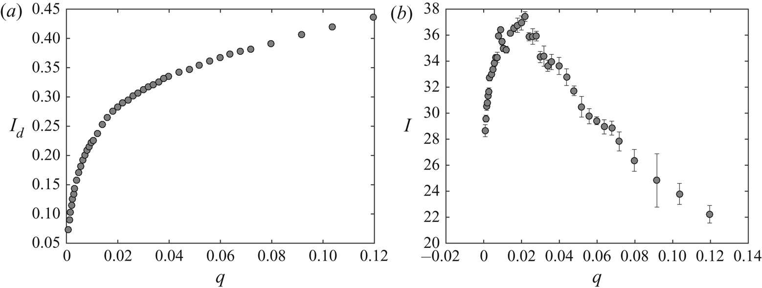
The electric charge  $\hat {{\mathcal {C}}}_d$ of the large droplets was measured in Hijano et al. (Reference Hijano, Loscertales, Ibáñez and Higuera2015) and found to be approximately 25 % of the Rayleigh limit charge
 $\hat {{\mathcal {C}}}_{R}=8 {\rm \pi}(\epsilon _0 \gamma \hat {d}_d^3)^{1/2}$. The mean dimensionless electric current carried by the large droplets (scaled with
 $(\epsilon _0 \gamma ^2/\rho )^{1/2}$) is thus
 $I_d \approx 6.28 \, f d_d^{3/2}$, which is shown in figure 16(
 $a$). This current is one order of magnitude smaller than the total mean current reaching the collector, also obtained from experimental measurements in Hijano et al. (Reference Hijano, Loscertales, Ibáñez and Higuera2015), shown in figure 16(
 $b$), so the current must be mainly transported by other entities apart from the main droplets. If those were the droplets generated by the electrospray emitted from the conical tip, according to Fernández de la Mora & Loscertales (Reference Fernández de la Mora and Loscertales1994) the dimensionless current would be
 $I_s\approx g(\epsilon )\eta =g(\epsilon )(\hat {q}_s/\hat {q}_o)^{1/2}$, where
 $\hat {q}_s$ is the liquid flow rate of the electrospray,
 $\hat {q}_o= \gamma \epsilon _0 \epsilon /\rho K$ is a characteristic flow rate, and
 $g(\epsilon )$ is a dimensionless function of the permittivity of the liquid, which turns out to be
 $g\approx 18$ for liquids with relatively large permittivities, such as the ones used in our experiments. According to Fernández de la Mora & Loscertales (Reference Fernández de la Mora and Loscertales1994), the dimensionless flow rate
 $\eta$ is of order unity so the typical values of
 $I_s$ are in the range of the observed current.
Dimensionless mean current transported by large droplets  $I_d$ (
 $a$) and total mean current measured at the collector electrode
 $I$ (
 $b$) versus the dimensionless flow rate
 $q$, from experimental measurements. Results are shown for
 ${B_{E}}=3.72$,
 ${B}=6.3 \times 10^{-2}$ and
 ${Oh}=1.55\times 10^{-2}$.

In this case, a rough estimation of the electric field induced by the charge of the electrospray around the tip of the meniscus can be worked out as follows. The flow rate of the electrospray can be expected to be of the order of the minimum flow rate in the cone-jet mode. According to Fernández de la Mora & Loscertales (Reference Fernández de la Mora and Loscertales1994), this flow rate is approximately  $0.25 \, \hat {q}_o$, and the diameter of the spray droplets (approximately twice the diameter of the jet) is
 $\hat {d}_{sd} \approx 0.5 \, (\epsilon _0^2 \epsilon ^2 \gamma /\rho K^2)^{1/3} =24.6$ nm. The charge of these droplets may be a fraction 0.44 of their Rayleigh limit charge (Collins et al. Reference Collins, Sambath, Harris and Basaran2013), which amounts to
 $\hat {{\mathcal {C}}}_{sd}=2.58 \times 10^{-17}$ coulomb. The Cunningham factor for droplets of this size in air at normal conditions is
 $C \approx 10.04$, and their electrical mobility is
 $\hat {\nu }_{sd}= C {\mathcal {C}}_{sd}/(3 {\rm \pi}\mu _{air} \hat {d}_{sd})=6.17 \times 10^{-5}\ \textrm {m}^2\,\textrm {V}^{-1}\,\textrm {s}^{-1}$. The electric field at the axis of a Taylor cone is
 $\hat {E}_{T} \approx (\gamma /2 \epsilon _0 \hat {R})^{1/2}$ at a distance
 $\hat {R}$ from the apparent vertex of the cone. The electric field induced by the charge of the spray is also proportional to
 $\hat {R}^{-1/2}$, so that the total field can be written as
 $\hat {E}=(\gamma /2 \epsilon _0 \hat {R})^{1/2} a$, with
 $a$ to be found, and the droplets immersed in this field move with velocity
 $\hat {\nu }_{sd} \hat {E}$ in quiescent air. The value of
 $a$ was approximately computed by Fernández de la Mora (Reference Fernández de la Mora1992) assuming that the density of charge of the spray depends only on
 $R$. For a spray carrying an electric current
 $\hat {I}_s$ and spreading over a conical region of half-angle
 $\beta$, the result is
 $a=( {2 \hat {I}_s/[3 {\rm \pi}(1 - \cos \beta ) \hat {\nu }_{sd} \gamma ]})^{1/2}$. For
 $\hat {I}_s=200$ nA (from figure 16
 $b$, assuming that the mean current is due to electrospray emission during half of the oscillation period, see figure 10) and
 $\beta \approx 29^{\circ }$ (from the radius of the spray deposition spot on the collector), this gives
 $a \approx 0.36$, showing that the electric field induced by the charge of the spray around the tip of the meniscus significantly modifies the Taylor field.
5. Quantification of the reduction of the electric field at the conical tip due to electrospray emission
The effect of the electrospray emitted when the ligament of the equipotential meniscus develops a conical tip is further quantified in this section using the non-steady quasi-one-dimensional approximation of the Navier–Stokes equation introduced by Eggers & Dupont (Reference Eggers and Dupont1994) for slender menisci, combined with experimental information on the menisci profiles measured at consecutive times.
As in previous sections, we assume that the cone-to-jet transition region around the tip where charge transport phenomena take place, and the jet breakup length, are much smaller than any other length scale and, of course, much smaller than our optical resolution. This is based on the huge disparity between the characteristic time of the meniscus,  $t_c$, and the electrical relaxation time,
 $t_e$, as argued above, and on our experimental observations, where no jet can be identified with our current experimental set-up (spatial resolution of
 $5\,\mathrm {\mu }\textrm {m}$ per pixel). Therefore, in this scenario, the ultrafine electrospray is assumed to be directly emitted from the tip of an equipotential meniscus.
5.1. Mathematical model. One-dimensional approximation of the fluid dynamics
In the one-dimensional (1-D) approximation, the mass and momentum conservation equations for a viscous fluid with infinite conductivity subjected to an electric field are (Hohman et al. Reference Hohman, Shin, Rutledge and Brenner2001; Ibáñez Reference Ibáñez2015)
 $$\begin{gather} \frac{\partial h^2}{\partial t}+\frac{\partial}{\partial x}\left(h^2u\right)=0, \end{gather}$$
 $$\begin{gather}\frac{\partial u}{\partial t}+u\frac{\partial u}{\partial x}={-}\frac{\partial}{\partial x} {\left( {\kappa-\frac{{B_{E}}}{2} E^2}\right)} +3\frac{{Oh}}{h^2} \frac{\partial}{\partial x} \left(h^2\frac{\partial u}{\partial x}\right) +{B} , \end{gather}$$
where  $h(x,t)$ and
 $u(x,t)$ are the dimensionless radius of the meniscus and the dimensionless velocity of the liquid. We look for time-periodic solutions of these equations satisfying the boundary conditions
 \begin{equation} \left. \begin{gathered} h(0,t)=\tfrac{1}{2} , \quad u(0,t)=v_o , \\ h(\ell,t)= 0 , \quad u(\ell,t) < \infty , \end{gathered} \right\} \end{equation}
where  $v_o=(4/{\rm \pi} ) q$ is the dimensionless average velocity of the flow feeding the meniscus and
 $\ell (t)$ is the instantaneous dimensionless length of the meniscus.
In (5.2),  $E$ is the electric field at the surface of the meniscus, which should be computed by solving
 \begin{equation} \boldsymbol{E}={-}\boldsymbol{\nabla} \phi_e , \quad \boldsymbol{\nabla}^2 \phi_e ={-}\rho_e, \end{equation}
with  $\phi _e=1$ at the tube and the surface of the meniscus and
 $\phi _e=0$ at the collector electrode. Here
 $\rho _e(\boldsymbol {x},t)$ is the dimensionless density of space charge in the gas due to the small droplets of the spray emitted from the tip of the meniscus. In this section, rather than finding
 $\rho _e$ and solving the electric problem, the electric field and the electric stress at the surface of the meniscus will be evaluated using the distribution of meniscus radius
 $h$ measured in the experiment.
For the treatment of the mechanical problem (5.1)–(5.3), it is convenient to rescale the axial distance  $x$ with the meniscus length,
 $\ell$, which changes with time as the meniscus evolves. In terms of the rescaled axial distance
 $z=x/\ell$, which varies between 0 and 1, (5.1)–(5.3) become
 \begin{align} &\frac{\partial h^2}{\partial t} -\left(\frac{\dot{\ell}}{\ell}\right)z\frac{\partial h^2}{\partial z} +\left(\frac{1}{\ell}\right)\frac{\partial}{\partial z}\left(h^2u\right)=0, \end{align}
 $$\begin{align} &\frac{\partial u}{\partial t}+\left[\left(\frac{1}{\ell}\right)u -\left(\frac{\dot{\ell}}{\ell}\right)z\right]\frac{\partial u}{\partial z}={-}\left(\frac{1}{\ell}\right)\frac{\partial}{\partial z}{\left( { \kappa-\frac{{B_{E}}}{2} E^2}\right)} \nonumber\\ &\quad +3\left(\frac{{Oh}}{\ell^2}\right) \frac{1}{h^2}\frac{\partial}{\partial z}\left( { h^2\frac{\partial u}{\partial z} }\right) + {B} , \end{align}$$
 \begin{align} &\left. \begin{gathered} h(0,t)=\tfrac{1}{2} , \quad u(0,t)=v_o , \\ h(1,t)= 0 , \quad u(1,t) < \infty . \end{gathered} \right\} \end{align}
Here  $\dot {\ell }=\mathrm {d} \ell /\mathrm {d} t$.
5.2. Computing the electric field on the meniscus surface
Since the distribution of space charge around the meniscus is not known, the 1-D model sketched above can be used only in combination with experimental data to obtain the dimensionless electric field on the meniscus surface,  $E(z,t)$. This is done as follows.
From the experiments, we can measure the meniscus profile  $h(z,t)$ and the length
 $\ell (t)$ at several consecutive times, so that the quantities
 $\partial h/\partial t$ and
 $\dot {\ell }(t)$ can be computed. Our system allows a resolution of
 $5\ \mathrm {\mu }\textrm {m}$ per pixel, which provides an error on the measurements of
 $h$ and
 $\ell$ of less than
 $2\,\%$. Each meniscus profile is discretized using 1000 points. The time step between consecutive frames may be as small as
 $2.63\times 10^{-5}$ s, which amounts to
 $\delta t \approx 9 \times 10^{-3}$ in dimensionless variables. We compute the time derivatives with a precision of
 $O(\delta t^2)$.
Using these data, we numerically integrate with respect to  $z$ the mass conservation equation (5.5) to obtain the dimensionless local flow rate
 $\tilde {q} = {\rm \pi}h^2 u$ up to an integration constant that depends on time. The way this constant is determined deserves some discussion. According to the 1-D model, the local flow rate
 $\tilde {q}(z,t)$ must satisfy simultaneously
 $\tilde {q}=({\rm \pi} /4) v_o$ at
 $z=0$ and
 $\tilde {q}=0$ at
 $z=1$, since
 $h(1,t)=0$ and
 $u(1,t)$ remains finite. However, the condition at
 $z=0$ is hard to use for the following reasons. First, the experimental profiles are obtained with slight uncertainties associated mainly with some lack of symmetry, to possible misalignment between the axis of the meniscus and that of the video camera, and to the finite resolution of the video frame (i.e. pixelation). To increase precision, a subpixel detection method has also been implemented, which consists of fitting a sigmoid function to the grey intensity level across the edge in each point of the meniscus (Acero et al. Reference Acero, Ferrera, Montanero, Herrada and López-Herrera2013; Hijano et al. Reference Hijano, Loscertales, Ibáñez and Higuera2015). All of previous uncertainties may lead to a violation of the mass conservation equation between consecutive frames (the mass emitted by the invisible aerosol is much smaller and plays no role in this regard); since
 ${\rm \pi} h^2 \mathrm {d} z$ is the volume of a slice of the meniscus of radius
 $h$, the experimental errors of the volume are amplified at larger values of
 $h$, that is, near the tube exit. Second, it is not always easy to detect the point at which the meniscus touches the needle. Third, the velocity of the fluid exiting the capillary tube has a parabolic profile (provided the Reynolds number of the flow in the tube is below 2200) rather than the flat profile assumed in the 1-D model. As a consequence, the 1-D model does not reproduce the experimental shape of the meniscus near the needle (Yildirim & Basaran Reference Yildirim and Basaran2001). The length required to flatten out the axial velocity profile may be estimated by considering the adaptation length in a tube,
 $\hat {L}_a$, given by
 $\hat {L}_a/D \sim \rho \hat {q}/(\mu D)$, which reads
 $\hat {L}_a/D \sim q/{Oh}$ in terms of the dimensionless flow rate
 $q$ and the Ohnesorge number. This length is not small in our experiments. Due to these issues, the results of the 1-D model are expected to depart from the experimental results near the tube, and the condition
 $\tilde {q}=({\rm \pi} /4) v_o$ can hardly be satisfied at
 $z=0$.
At the meniscus tip the measurement errors are also present, but in contrast to  $h(0,t)$, the tip
 $h(1,t)=0$ is easily identified experimentally, and its axial position in time,
 $\ell (t)$ is easily measured, so we have chosen the condition
 $h^2 u=0$ at
 $z=1$ to fix the integration constant that yields
 $\tilde {q}(z,t)$. Even though the meniscus might cease being slender around its tip, particularly when the meniscus nose is rounded, we are interested in menisci having pointed conical tips, where the slenderness might still be enough (we shall see that the cone semiangle in our experiments is approximately
 $37^{\circ }$) and, on the other hand, Eggers & Dupont (Reference Eggers and Dupont1994) and Yildirim & Basaran (Reference Yildirim and Basaran2001) argue that the 1-D model still provides good results for rounded menisci if they are approximately hydrostatic. This is because the capillary stresses (and the electric stresses in our case) are exactly represented in the model, so equilibrium and quasi-equilibrium shapes are actually well reproduced. From
 $\tilde {q}(z,t)={\rm \pi} h^2(z,t) u(z,t)$,
 $u(z,t)$ can be computed. By repeating this procedure with profiles measured at consecutive times we compute
 $u(z,t)$ at consecutive instants, and then also
 $\partial u/\partial t$,
 $\partial u/\partial z$ and
 $\partial ^2 u/\partial z^2$, evaluating all the spatial derivatives with precision of
 $O(\mathrm {d} z^2)$ after using least-squares spline interpolation to smooth the measured contour of the meniscus.
Figure 17 shows five digitalized dimensionless meniscus profiles recorded at five consecutive dimensionless times,  $0$,
 $0.0785$,
 $0.1570$,
 $0.2358$ and
 $0.3139$, respectively. They capture the early stages of the neck formation during one cycle. In this example
 ${B_{E}}=3.72$,
 ${B}=6.3 \times 10^{-2}$,
 ${Oh}=1.55 \times 10^{-2}$ and
 $v_o=6.12\times 10^{-3}$. The axial distance is normalized with the instantaneous dimensionless length
 $\ell$ (also measured from the video frames). Each profile consists of 1000 points.
Dimensionless meniscus profiles  $h$ versus
 $z$ for
 ${B_{E}}=3.72$,
 ${B}=6.3 \times 10^{-2}$,
 ${Oh}=1.55 \times 10^{-2}$ and
 $v_o=6.12\times 10^{-3}$. The dimensionless times elapsed from the first profile are 0.0785, 0.1570, 0.2358 and 0.3139, respectively.

Figure 18 shows  $h^2 u$ (a) and
 $u$ (b) versus
 $z$ at times 0.0785, 0.1570 and 0.2358. The figure also shows
 $\partial (h^2 u)/\partial t$ (c) and
 $\partial u/\partial t$ (d) versus
 $z$ at time 0.1570, obtained from data in figure 17. Figure 18(
 $a$) shows
 $h^2 u$ obtained from the numerical integration of the mass conservation equation applied to the experimental profiles. Note that we have forced
 $h^2 u=0$ at
 $z=1$, so that
 $h^2 u \neq v_o/4$ at
 $z=0$ in all the cases, exhibiting relatively large differences due to inaccuracies in the measurements of
 $h(z,t)$. These departures from the correct boundary condition at
 $z=0$ are even larger for rounded menisci (not shown), for which the limited resolution of the video frames leads to relatively large errors in computing the volume of the experimental meniscus. Also, it is important to notice that we can only integrate the mass conservation equation on
 $t=0.0785$, 0.1570 and 0.2354 since we used centred (time) differences to compute time derivatives. Figure 18(
 $b$) shows the corresponding velocity profiles for these three times, where the tip velocity is experimentally obtained from the measurement of
 $\ell$ with time. Figure 18(
 $c$,
 $d$) shows
 $\partial (h^2 u)/\partial t$ and
 $\partial u/\partial t$, respectively. The latter are calculated only at
 $t=0.1579$.
Plots of  $h^2 u$ (
 $a$) and
 $u$ (
 $b$) versus
 $z$ at times
 $0.0785$,
 $0.1570$ and
 $0.2358$,
 $\partial (h^2 u)/\partial t$ (
 $c$) and
 $\partial u/\partial t$ (
 $d$) versus
 $z$ at time
 $0.1570$. Results are shown for
 ${B_{E}}=3.72$,
 ${B}=6.3 \times 10^{-2}$,
 ${Oh}=1.55 \times 10^{-2}$ and
 $v_o=6.12\times 10^{-3}$.

The next step is to turn to the axial momentum equation (5.6), where everything is now known except the pressure gradient,  $\partial {(\kappa - {B_{E}} E^2/2)}/\partial z$. Therefore, we numerically integrate (5.6) over
 $z$ to obtain the pressure distribution
 $\kappa - {B_{E}} E^2/2 + C(t)$, where
 $C(t)$ is another integration constant that depends on time. Since the meniscus profile is known experimentally, the curvature
 $\kappa$ can be evaluated, so that the only unknowns left are the electric field
 $E$ and the constant
 $C$. To evaluate
 $C$ we should know the value of the electric pressure at some point on the meniscus surface. Since this information is not experimentally available, we fix
 $C$ by assuming that, far from the tip, the effect of the space charge due to the electrospray emitted from the tip is small, so that
 $E=|\boldsymbol {\nabla } \phi _e|$ with
 $\boldsymbol {\nabla }^2 \phi _e=0$; i.e. the electric field away from the meniscus tip coincides with the electric field computed with the BEM method without any space charge. Figure 19 shows the values of the pressure,
 $p=\kappa -{B_{E}} E^2/2 + C$ and the capillary pressure,
 $p_{\gamma }=\kappa$ computed from the data in figure 18.
Dimensionless total pressure,  $p=\kappa -{B_{E}} E^2/2+C$ (
 $a$), and dimensionless capillary pressure,
 $p_{\gamma }=\kappa$ (
 $b$), versus the axial coordinate
 $z$ at
 $t=0.157$.

It is interesting to notice that the capillary pressure,  $p_{\gamma }$, which is of the order of the electric pressure, becomes much larger than
 $p$ as the conical tip of the ligament is approached (see figure 19), whereas the inertia term at the tip,
 $\partial u/\partial t$ (see figure 18
 $d$), remains of the order of
 $p$. This result indicates that, near the conical tip of the ligament, the fluid behaves approximately as if it were at electrohydrostatic equilibrium. Therefore, even though the conical tip might not be slender, the arguments raised by Eggers & Dupont (Reference Eggers and Dupont1994) and Yildirim & Basaran (Reference Yildirim and Basaran2001) to support the 1-D approximation also hold in our case.
Figure 20 shows the electric field at the meniscus computed using the BEM and the combination of the 1-D model and the experimental profiles for three different cases, with the constant  $C$ evaluated as described above. The figure also includes the instantaneous shape of the meniscus, rescaled radially to facilitate visualization. The solid curve is the meniscus profile, the dash–dotted curve is the electric field computed with the BEM method (that is, assuming there is no space charge) and the dashed curve is the electric field obtained using the 1-D model. In all the cases
 ${B}=6.3\times 10^{-2}$ and
 ${Oh}=1.55\times 10^{-2}$. In figure 20(a)
 ${B_{E}}=4.96$ and
 $v_o=6.12\times 10^{-3}$, while figure 20(
 $b$,
 $c$) shows results for
 ${B_{E}}=3.76$ and
 $v_o=10.71\times 10^{-3}$ at two instants during the oscillation cycle. Cases if figure 20(
 $a$,
 $c$) exhibit sharp tips whereas the case in figure 20
 $(b)$ corresponds to a rounded meniscus, as shown.
Electric field  $E$ versus the axial coordinate
 $z$ for three different situations. Dash–dotted line, electric field computed with the BEM; dashed line, electric field obtained from the integration of the 1-D model; solid line, the meniscus profile. Results are shown for (a)
 ${B_{E}}=4.96$ and
 $v_o=6.12\times 10^{-3}$, (
 $b$,
 $c$)
 ${B_{E}}=3.76$ and
 $v_o=10.71\times 10^{-3}$. In all cases
 ${B}=6.3\times 10^{-2}$ and
 ${Oh}=1.55\times 10^{-2}$.

It is interesting to note that in figure 20 $(b)$, where there is no sharp tip, the values of the electric field obtained from the BEM and the 1-D model are nearly equal to each other throughout the meniscus surface, particularly at the meniscus nose. The small differences are probably due to the limitations on the measurements of the profile mentioned in previous sections, and perhaps also to the lack of slenderness in this meniscus. This result strongly suggests that while the meniscus tip stays rounded there is no space charge near the meniscus. On the other hand, when the sharp tip appears, such as in cases in figure 20(
 $a$,
 $c$), the values of the electric field computed by the BEM and the 1-D model are nearly identical far from the tip but become rather different as the tip is approached. In fact, the field computed by the 1-D model is systematically smaller than the one computed by BEM. This is consistent with the presence of a relatively intense space charge near the meniscus tip, which would be caused by the emission of an ultrafine electrospray from the tip of the liquid ligament.
5.3. Relationship between the electric field at the conical tip and the tip semiangle
The magnitude of the effect of such ultrafine electrospray on the electric field at a conical meniscus may be estimated following the work of Fernández de la Mora (Reference Fernández de la Mora1992). This author analytically describes an extension of the hydrostatic solution for an electrified conical meniscus given by Taylor (Reference Taylor1964) by introducing a conical inertialess charged spray of semiangle  $\beta$ that is emitted from the tip of the static electrified conical meniscus of semiangle
 $\alpha$. The presence of this charged spray alters the original solution given by Taylor, in which the conical meniscus has a semiangle
 $\alpha _T=49.23^{\circ }$, yielding values of
 $\alpha$ smaller than
 $\alpha _T$, as regularly observed experimentally. Even though Fernández de la Mora (Reference Fernández de la Mora1992) does not provide the explicit expression of the electric field at the surface of the conical meniscus,
 $E^*$ say, it may be easily computed from the solution given there, resulting in dimensionless form in
 \begin{equation} E^*=\left(\frac{2}{{B_{E}}}\right)^{1/2}\frac{F(\alpha)}{R^{1/2}}, \end{equation}
where  $R$ is the dimensionless distance to the tip of the conical meniscus and
 $F(\alpha )$ is a known combination of Legendre functions. In brief, as the charged aerosol becomes more intense
 $\alpha$ decreases.
That the electric field in a region around the conical tip varies as  $R^{-1/2}$ is not clear at this point. To check this assumption we represent in figure 21 the electric field on the surface of the meniscus calculated by using the 1-D model,
 $E$, versus
 $R$, the dimensionless distance measured from the apex of the tip to the point on the surface of the tip of the meniscus where the electric field is obtained. Also, figure 21 includes a fitting of the data with an
 $R^{-1/2}$ dependence with the origin shifted 0.01 to account for the misallocation of the virtual apex due the limitations of our optical system. Except for the noisy points at the very tip
 $R\rightarrow 0$ due to the limitations of our experimental system, the data suggest that the electric field on the menisci goes approximately as
 $R^{-1/2}$ during a relatively large part of the conical tip of the ligaments, as assumed in Fernández de la Mora (Reference Fernández de la Mora1992). Therefore, one would expect a relationship between the value of the group
 \begin{equation} \left(\frac{{B_{E}}R}{2}\right)^{1/2}E \end{equation}
and the conical tip semiangle  $\alpha$, as suggested by (5.8).
Plot of  $E$ versus
 $R$ measured from the tip for cases in figure 20
 $(a)$, circles, and
 $(c)$, diamonds. The dashed line is proportional to
 $R^{-1/2}$.

We have measured the semiangle  $\alpha$ of the conical tips that form during the evolution of the oscillating meniscus for three dimensionless flow rates,
 $q=2.4\times 10^{-4}$,
 $2.4\times 10^{-3}$ and
 $2.4\times 10^{-2}$, with
 ${B}=1.2\times 10^{-1}$,
 ${Oh}=1.55 \times 10^{-2}$, and several values of
 ${B_{E}}$, and have computed the corresponding values of the electric field around the tip rescaled as in (5.9), where
 $E$ is obtained from the 1-D model as explained above.
To measure the semiangle  $\alpha$ we fit a line to the 10 points (pixels in the image) closer to the tip of the meniscus contour detected in each frame of the recorded experimental videos. If there is spray emission in the frame being considered, the tip of the meniscus has a conical shape and the fitting of a line to the last 10 points of the tip is good. A fitting is accepted if the R-square value of the linear regression is higher than 0.96. Then the angle
 $\alpha$ is measured between the fitted line and the centreline of the meniscus.
The results, along with the prediction of (5.8), are shown in figure 22. For all the experimental conditions, the values of  $\alpha$ remains within
 $37\pm 5 ^{\circ }$, and the values of the rescaled electric fields, which are scattered around unity, are in surprisingly good agreement with the predictions of Fernández de la Mora (Reference Fernández de la Mora1992). This is despite the fact that our conical menisci are not steady and despite all the errors in the measurements of
 $\alpha$ and the approximations in computing
 $E$. On one hand, this agreement gives support to the scheme we have followed to compute
 $E$ for the experimental meniscus and, on the other hand, indicates that the effect of the ultrafine electrospray emitted from the pointed meniscus is of paramount importance to describe the evolution of a relatively large portion of the ligament, even in the case of an infinitely conducting liquid. Furthermore, it also indicates that the details of the cone-to-jet transition region and the jet breakup length that must exist at the inception of the ultrafine electrospray on the conical tip and involve complicated charge transport processes, do not affect the dynamics of the oscillating meniscus for the case of highly conducting liquids.
Rescaled normal electric field  $(R{B_{E}}/2)^{1/2}E$ versus the semiangle of the conical tip
 $\alpha$ for three different flow rates and several
 ${B_{E}}$. The line is the prediction from (5.8). For
 $q=2.4\times 10^{-4}$: squares,
 ${B_{E}}=4.0$; diamonds,
 ${B_{E}}=4.5$; circle,
 ${B_{E}}=5.9$. For
 $q=2.4\times 10^{-3}$: upward-pointing triangles,
 ${B_{E}}=4.1$; crosses,
 ${B_{E}}=5.0$; plus sign,
 ${B_{E}}=7.0$; pentagram,
 ${B_{E}}=7.2$. For
 $q=2.4\times 10^{-2}$: hexagrams,
 ${B_{E}}=4.5$; asterisks,
 ${B_{E}}=5.2$; downward-pointing triangles,
 ${B_{E}}=7.6$. In all cases
 ${B}=1.2\times 10^{-1}$ and
 ${Oh}=1.55 \times 10^{-2}$.

6. Conclusions and future work
The present research introduces a simple model to simulate the dynamics of a meniscus of a highly conducting, low viscosity liquid sticking out of a capillary needle when it is subjected to an intense electric field. The electric field is set by applying an electric potential difference between the capillary needle and a flat metallic plate placed in front of the needle (needle–plate configuration). In particular, the aim is to model the so-called axial mode II of Juraschek & Röllgen (Reference Juraschek and Röllgen1998), an oscillating regime in which the meniscus elongates, forming a liquid ligament that upon pinch-off forms a single droplet per oscillation.
This basic model assumes the liquid to be a perfect conductor,  $K\rightarrow \infty$, and inviscid,
 $\mu =0$, so the velocity may be written in terms of a velocity potential,
 $\hat {\boldsymbol {v}}=\boldsymbol {\nabla }\hat {\phi }$, that must satisfy the Laplace equation,
 $\boldsymbol {\nabla }^2\hat {\phi }=0$. The electric potential outside the liquid is assumed to satisfy the Laplace equation,
 $\boldsymbol {\nabla }^2\hat {\phi }_e=0$. The interaction between the fields occurs across the liquid surface. For a fixed electrode geometry, the problem is governed by three dimensionless parameters: the electric Bond number,
 ${B_{E}}$, the dimensionless flow rate,
 $q$, and the gravitational Bond number,
 ${B}$. The problem is solved by using the BEM.
The numerical results show that the assumptions taken by Hijano et al. (Reference Hijano, Loscertales, Ibáñez and Higuera2015) to perform their asymptotic analysis are basically correct.
The model has been compared with the experiments carried out by Hijano et al. (Reference Hijano, Loscertales, Ibáñez and Higuera2015), with conducting water solutions operating in the axial mode II, so-called electric microdripping regime.
The simulations capture the dependence of the oscillation frequency,  $f$, and mean volume,
 $V_{M}$, with the dimensionless flow rate,
 $q$, but overestimate the former by
 $40\,\%$ at most and underestimate the later by a similar amount.
The reason behind the discrepancy is twofold. The experiments show that during a non-negligible part of the life of the ligament extending from the meniscus, a conical tip forms. This Taylor cone emits a very thin jet that yields a stream of tiny, highly charged droplets. Therefore, an intense volumetric charge density exists. On one hand, the fluid might cease to be equipotential near the vertex of the Taylor cone, where the jet forms, and therefore one of the assumptions breaks down. On the other hand, the electrospray emitted from the cone tip constitutes a volumetric charge density between the meniscus and the collector whose intensity and location are unknown. In fact, the presence of the space charge limits the strength of the electric field pulling the liquid ligament, as measured from the experiments, whereas in the computations the electric field pulling the ligament grows well beyond this limiting value since there is no allowance for any space charge. This spurious electric pulling is able to tear off a certain mass of fluid while the ligament evolves.
As a consequence, the shape and lengths of the ligaments obtained from the model are larger and thinner than those in the experiments, respectively, and the volume of the ligament that pinches-off is smaller than the experimental one. Also, the minimum flow rate at which the axial mode II changes into the axial mode I is overestimated by the simulations; this is also explained in terms of the spurious mass ejection.
Although the mean averaged volume emitted by the oscillating meniscus is well captured by the model, the details of the electrohydrodynamics of these oscillating meniscus require the inclusion of the space charge due to the electrospray emitted from the cone tip and also the effect of the finite conductivity.
We have used a combination of the 1-D approximation of the Navier–Stokes equations introduced by Eggers & Dupont (Reference Eggers and Dupont1994) and experimental meniscus profiles to compute the normal electric field along the meniscus surface at different stages of its evolution. When the meniscus is pointed, the computed field becomes considerably smaller than the one computed by BEM, thus unravelling the effect of the emitted ultrafine electrospray. The newly computed normal electric field near the meniscus conical tip is in agreement with the asymptotic description of a conical meniscus emitting a conical electrospray made by Fernández de la Mora (Reference Fernández de la Mora1992). This could be used in the future to include in the modelling an approximate effect of this ultrafine electrospray.
Funding
This work has been supported by the Spanish Red Nacional para el Desarrollo de la Microfluídica (MIFLUNET) through project DPI2015-71901-REDT, RED2018-102829-T and by the Spanish Ministerio de Ciencia, Innovación y Universidades through grants DPI2017-86547-C2-1-P and DPI2017-86547-C2-2-P. The authors thank the Supercomputing Center of Universidad de Málaga (SCBI) for computational facilities and support.
Declaration of interests
The authors report no conflict of interest.
Author contributions
A.J.H. performed the experimental measurements, and A.J.H., I.G.L. and F.J.H. derived the theory and performed the computations. All authors contributed equally to analysing data and reaching conclusions, and in writing the paper.