1. Introduction
This paper advances the study of boundary-layer transition over rotating cones. Specifically, we consider the convective instability of a slender rotating cone of half-angle
 $15^{\circ }$
placed in oncoming uniform axial flows of various strengths. While the model presented is valid for other slender half-angles in the range up to approximately
 $40^{\circ }$
, a half-angle of
 $15^{\circ }$
is chosen as a representative value for definiteness and to facilitate comparison with existing results in the literature by Kobayashi, Kohama & Kurosawa (Reference Kobayashi, Kohama and Kurosawa1983).
The article forms part of a series of studies which have used theoretical techniques to construct the correct models of governing instability for both broad and slender rotating cones. The current study represents a significant extension to the general problem in the slender cone case, introduced when enforcing an oncoming axial flow.
Physically, the problem represents an accurate model of flow over a rotating conical projectile, such as the nose of a spinning sharp missile. Here laminar–turbulent transition within the boundary layer can lead to significant increases in drag, which has negative implications for fuel efficiency, control and accurate missile-targeting. In such cases, delaying transition to turbulent flow is seen as beneficial, and controlling the primary instability may be one route to achieving this. Ultimately, control of the input parameters of such a problem may lead to design modifications and potential cost savings.
The purpose of applying a linear stability analysis in such a study is to reveal the effect of varying the governing control parameter, namely the ratio of oncoming flow to rotational flow. While the current authors have conducted cross-flow stability analyses of the effects of enforced axial flow over broad rotating cones and disks (see Garrett & Peake Reference Garrett and Peake2007; Garrett, Hussain & Stephen Reference Garrett, Hussain and Stephen2010; Hussain Reference Hussain2010; Hussain, Garrett & Stephen Reference Hussain, Garrett and Stephen2011), this paper represents the first such study to apply a centrifugal Görtler stability analysis to a slender cone rotating within an axial flow. As such, the investigation extends the work of Hussain, Garrett & Stephen (Reference Hussain, Garrett and Stephen2014), which presents a full description of the still-fluid problem. Specifically, we present a new and rigorous similarity solution for the basic flow, on which we perform a stability analysis, employing both asymptotic and numeric methods.
Importantly, in this paper we consider only stationary instabilities, which are the most easily observed in flow-visualisation experiments. While travelling modes, which move along the surface in the axial direction, have been shown to play an important role in the rotating-disk case (see Corke & Knasiak Reference Corke and Knasiak1998; Hussain et al. Reference Hussain, Garrett and Stephen2011), the slender-rotating-cone boundary layer is dominated by a different underlying centrifugal instability. Such travelling modes are neglected in the present study, but their effect on the flow may be considered in future investigations.
The paper is structured as follows. We begin by justifying the rationale for the choice of a new basic flow in § 2, proceeding to formulate the problem in § 3, using modified scalings to correctly model terms arising from the centrifugal instability. Subsequently we outline the asymptotic analysis in § 4 and the corresponding numerical analysis in § 5, along with the major differences between the two solution methods. The results of the two theoretical analyses are compared in § 6, as well as with other numerical and experimental studies in the literature. Finally, conclusions are drawn in § 7.
2. Justification of the centrifugal mode and updated basic flow
We begin by discussing the rationale for the choice of an alternative instability mechanism for slender rotating cones, as well as the reasons for using a modified basic flow field.
First, flow visualisation studies of flow over slender rotating cones by Kobayashi et al. (Reference Kobayashi, Kohama and Kurosawa1983) (axial flow) and Kobayashi & Izumi (Reference Kobayashi and Izumi1983) (still fluid) show that the primary instability is characterised by pairs of counter-rotating Görtler vortices. However, as the half-angle
 ${\it\psi}$
is increased beyond
 $40^{\circ }$
, their visualisations clearly show that these vortices change to co-rotating vortices, as observed on rotating disks by Gregory, Stuart & Walker (Reference Gregory, Stuart and Walker1955), Kohama (Reference Kohama1985), Reed & Saric (Reference Reed and Saric1989), Kobayashi (Reference Kobayashi1994), Corke & Knasiak (Reference Corke and Knasiak1998), Saric, Reed & White (Reference Saric, Reed and White2003), for example. It has been proposed by Garrett, Hussain & Stephen (Reference Garrett, Hussain and Stephen2009) and Hussain et al. (Reference Hussain, Garrett and Stephen2014) that the counter-rotating vortices are expected to arise from a dynamic instability induced by the centrifugal force of the flow field, and the co-rotating vortices are attributed to an underlying cross-flow instability. The existence of an alternative mode of instability to the cross-flow-dominated type I and type II modes used to model vortices on broad rotating cones was discussed in Garrett et al. (Reference Garrett, Hussain and Stephen2009). Subsequently, a consistent model to correctly characterise the dominant centrifugal-instability ‘Görtler’ mode for slender rotating cones has been applied successfully by Hussain et al. (Reference Hussain, Garrett and Stephen2014) in the still-fluid case. Therefore, both experimental observations and theoretical predictions provide evidence for the existence of distinct governing instability mechanisms over slender and broad cones.
Secondly, the physical problem of superposing an oncoming axial flow onto a rotating cone in still fluid depends on two important velocities: the rotational speed of the cone surface and the local tangential slip velocity at the edge of the boundary layer, which is directly related to the strength of the oncoming axial flow. The ratio of these two velocities defines whether the cone is rotating ‘quickly’ (with a larger rotational velocity) or ‘slowly’ (with a larger oncoming flow). Specifically, we consider cases where the oncoming uniform axial flow is increased gradually from zero (starting from initially still fluid), so the flow setup corresponds to the former case above of a cone rotating ‘quickly’. Importantly, we note that this is not a single unsteady problem but rather a sequence of steady ones, each of which is characterised by a different strength of oncoming axial flow. Existing studies have computed the basic flow for this problem, with Garrett et al. (Reference Garrett, Hussain and Stephen2010) displaying accurate solutions for
 $50^{\circ }$
and
 $70^{\circ }$
half-angle cones. We note that this study adopted a new method of similarity solution in terms of the governing stream-function, which resolved problems in the basic flows originally proposed by Garrett & Peake (Reference Garrett and Peake2007). Furthermore, the earlier basic flow solutions proposed by Kobayashi (Reference Kobayashi1981) and later used in the theoretical analysis of Kobayashi et al. (Reference Kobayashi, Kohama and Kurosawa1983) appear to show some deviation from convergent behaviour at the edge of the boundary layer. Results are given for a range of spiral wave angles, in order to recover the case which more closely represents experimental results. Basic flow solutions presented by both Kobayashi (Reference Kobayashi1981) and Garrett et al. (Reference Garrett, Hussain and Stephen2010) apply a method which is similar to that used by Koh & Price (Reference Koh and Price1967). However, the new solutions presented by Garrett et al. (Reference Garrett, Hussain and Stephen2010) require only specification of the cone half-angle and the governing ratio of the two characteristic flow velocities in order to produce solutions exhibiting fully convergent behaviour at the edge of the boundary layer. It is for this reason that we apply this updated formulation to obtain new basic flow solutions for a
 $15^{\circ }$
half-angle cone in a range of axial flows.
Importantly, for very slender cones
 $({\it\psi}\leqslant 15^{\circ })$
, Kobayashi & Izumi (Reference Kobayashi and Izumi1983), Kobayashi et al. (Reference Kobayashi, Kohama and Kurosawa1983) have observed both spiral and circular vortices for cones rotating in axial flow and still fluid, respectively. These are distinguished by non-zero and zero wave angles. For the still-fluid problem, the theoretical study of these two cases differs depending on the orientation of the spiral vortices, with the circular wave case of
 ${\it\psi}\leqslant 15^{\circ }$
being analysed by Hussain, Stephen & Garrett (Reference Hussain, Stephen and Garrett2012), while the case of spiral vortices is presented by Hussain et al. (Reference Hussain, Garrett and Stephen2014). However, in the present study for a
 $15^{\circ }$
cone rotating in an enforced axial flow, the formulation in § 3 covers both circular and spiral vortices, depending on the wave angle parameter, which is essentially determined by the ratio of the oncoming flow speed to the rotational speed of the cone surface.
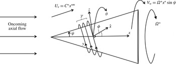
Diagram of the spiral vortex instability on a rotating cone placed in an oncoming axial flow, showing coordinates in the
 $\hat{x}$
- and
 $y$
-logarithmic spiral directions, as well as the corresponding vortex wavenumber,
 ${\it\gamma}$
, and vortex wave angle,
 ${\it\phi}$
. The problem is characterised by the relative strengths of the streamwise slip velocity at the edge of the boundary layer,
 $U_{e}$
, and the rotational speed of the cone surface,
 $V_{w}$
, which are encapsulated in the axial flow or rotational flow parameters,
 $T_{s}$
and
 $s$
, respectively.

3. Formulation
We consider a cone of half-angle
 ${\it\psi}$
rotating in a fluid of kinematic viscosity
 ${\it\nu}^{\ast }$
with an angular velocity
 ${\it\Omega}^{\ast }$
in an anti-clockwise direction around the streamwise coordinate axis
 $x^{\ast }$
(where a
 $^{\ast }$
denotes a dimensional quantity in all that follows). Other than the imposition of the axial flow, the formulation follows that detailed in Hussain et al. (Reference Hussain, Garrett and Stephen2014) and we construct coordinate axes aligned along and perpendicular to the spiral vortices (
 $\hat{x}^{\ast }$
and
 $y^{\ast }$
, respectively), as shown in figure 1. These are shifted from the conventional streamwise and azimuthal coordinates,
 $x^{\ast }$
and
 ${\it\theta}$
, that are based on cylindrical polar coordinates. In such a problem, there exists a boundary layer close to the rotating cone surface characterised by the distance along the cone
 $l^{\ast }$
and defined by the Reynolds number,
 $R$
, such that:
 $$\begin{eqnarray}R=\frac{{\it\Omega}^{\ast }l^{\ast 2}\sin {\it\psi}}{{\it\nu}^{\ast }}.\end{eqnarray}$$
However, we make the important distinction in this case by including an oncoming uniform axial flow. The physical problem is thus altered such that there now exists a dimensional local slip velocity at the edge of the boundary layer, which is obtained via a well-known potential-flow solution (see for example Rosenhead Reference Rosenhead1963 or Evans Reference Evans1968), given by
 $U_{e}=C^{\ast }x^{\ast m}$
, where
 $C^{\ast }$
is a constant and for a cone of half-angle
 $15^{\circ }$
considered in this study,
 $m=0.03927$
approximately.
We compare this velocity to the rotational velocity of the cone surface, given by
 $V_{w}={\it\Omega}^{\ast }x^{\ast }\sin {\it\psi}$
, to obtain two important ratios. These ratios fully characterise the problem, and are the local axial-flow parameter
 $$\begin{eqnarray}T_{s}=\frac{C^{\ast }x^{\ast m}}{{\it\Omega}^{\ast }x^{\ast }\sin {\it\psi}},\end{eqnarray}$$
used in the literature by Garrett & Peake (Reference Garrett and Peake2007), and the rotational-flow parameter given by
 $$\begin{eqnarray}s=\frac{1}{T_{s}^{2}}=\left(\frac{V_{w}}{U_{e}}\right)^{2},\end{eqnarray}$$
used earlier by Kobayashi (Reference Kobayashi1981) and Kobayashi et al. (Reference Kobayashi, Kohama and Kurosawa1983). In this study, we will predominantly use
 $s$
in order to facilitate comparison of our results with the experiments of Kobayashi et al. (Reference Kobayashi, Kohama and Kurosawa1983). However, we will make reference to
 $T_{s}$
where appropriate in physical cases where the cone is rotating ‘quickly’ and the axial flow is increased from a zero value.
In contrast to the axial flow problem for a rotating disk where
 ${\it\psi}=90^{\circ }$
analysed in Hussain et al. (Reference Hussain, Garrett and Stephen2011), the corresponding axial flow problem for a rotating cone with
 ${\it\psi}<90^{\circ }$
results in the solution of a system of partial differential equations (PDEs), with the basic flow velocities depending on both the streamwise and normal coordinates. Following Garrett et al. (Reference Garrett, Hussain and Stephen2010), we seek a similarity-type solution and utilise a Mangler transformation to capture the base flow quantities. The full details are provided in Garrett et al. (Reference Garrett, Hussain and Stephen2010) for
 ${\it\psi}=50^{\circ }$
and
 $70^{\circ }$
, and more completely in Hussain (Reference Hussain2010) for a range of values of
 ${\it\psi}$
. Here, we shall outline the important differences between the formulation for broad and slender half-angle cones in axial flow, and focus on the strategy of shifting the basic flow velocities from the well-known streamwise and azimuthal coordinates
 $x^{\ast }$
and
 ${\it\theta}$
to the new logarithmic coordinates along and normal to the spiral vortices
 $\hat{x}^{\ast }$
and
 $y^{\ast }$
.
We note that the shifted coordinate system
 $(\hat{x}^{\ast },y^{\ast },z^{\ast })$
rotates with the cone surface at the constant angular velocity
 ${\it\Omega}^{\ast }$
in order to aid the modelling of stationary disturbances over the cone surface. As in Hussain et al. (Reference Hussain, Garrett and Stephen2014), the logarithmic spirals are directed such that the
 $y^{\ast }$
-axis has a positive projection with the direction of rotation of the cone. This requires that the
 $\hat{x}^{\ast }$
-axis has positive projection onto the axis of rotation and the
 $y^{\ast }$
-axis has a negative projection, as shown in figure 1. The spiral vortices are orientated at an angle
 ${\it\phi}$
relative to the circle formed from the planar cross-sectional normal to the axis of rotation of the cone. Consequently, the governing dimensional Navier–Stokes equations are derived in this shifted coordinate system with appropriate scale factors.
We proceed to non-dimensionalise lengths on the distance along the cone
 $l^{\ast }$
, so that
 $\hat{x}^{\ast }=l^{\ast }\hat{x}$
and
 $y^{\ast }=l^{\ast }y$
. Furthermore, we scale both logarithmic coordinates
 $\hat{x}$
and
 $y$
, as well as the normal coordinate
 $z^{\ast }$
, on the boundary-layer thickness, leading to the scaled coordinate system
 $(\check{x},\bar{y},{\it\eta})=R^{1/2}(\hat{x},y,z)$
.
As for the still-fluid problem, this scaling is imperative to enable the vortex structure in both logarithmic directions to be analysed at the same order as the length scale in the surface-normal direction. This is because the counter-rotating Görtler vortices are characterised by both logarithmic coordinates, and so, as in Hussain et al. (Reference Hussain, Garrett and Stephen2014), we require this scaling to reveal their growth-dependent behaviour in each direction. Interestingly, for rotational flow parameter values
 $s\geqslant 5$
on a
 $15^{\circ }$
rotating cone, experimental studies by Kobayashi et al. (Reference Kobayashi, Kohama and Kurosawa1983) observe circular ‘Taylor’ waves (
 ${\it\phi}=0^{\circ }$
), as opposed to the more general spiral vortices. Nevertheless, the current formulation is able to model both spiral and circular waves, as we include the assumption that the spiral vortices exist and have a corresponding orientation angle
 ${\it\phi}$
. Therefore, setting
 ${\it\phi}=0^{\circ }$
pertains to the circular wave case.
Importantly, the basic flow quantities
 $\tilde{U}$
and
 $\tilde{V}$
are expressed as projections along the shifted spiral coordinates. However, due to the introduction of an oncoming axial flow, these are now functions of both the non-dimensional streamwise and surface-normal coordinates,
 $x$
and
 $z$
, respectively (where
 $x$
is the streamwise direction over the cone, scaled on
 $l^{\ast }$
). Hence, obtaining the base flows now requires the solution of a system of PDEs (see Garrett et al.
Reference Garrett, Hussain and Stephen2010; Hussain Reference Hussain2010 for full details and discussion) as opposed to the projected von Kármán solution of a system of ordinary differential equations (ODEs) presented in Hussain et al. (Reference Hussain, Garrett and Stephen2014) for the still-fluid problem. We also note from Hussain (Reference Hussain2010) that the basic flow solution to the boundary-layer equations for this problem has a correction of
 $O(R^{-1/2})$
. While there exist similar numerical basic flow formulations used by Kobayashi (Reference Kobayashi1981) and Kobayashi et al. (Reference Kobayashi, Kohama and Kurosawa1983), experimental verification of the basic flow is currently planned by R. Lingwood (personal communication, 2015). The shifted basic flow quantities are written correctly in the form:
 $$\begin{eqnarray}\displaystyle \tilde{U} (x,{\it\eta}) & = & \displaystyle U(x,{\it\eta})\cos {\it\phi}+V(x,{\it\eta})\sin {\it\phi},\end{eqnarray}$$
 $$\begin{eqnarray}\displaystyle \tilde{V}(x,{\it\eta}) & = & \displaystyle U(x,{\it\eta})\sin {\it\phi}+V(x,{\it\eta})\cos {\it\phi}.\end{eqnarray}$$
 $U(x,{\it\eta})$
and
 $V(x,{\it\eta})$
can be expressed in terms of the solution functions
 $f^{\prime }(s,{\it\eta}_{1})$
and
 $g(s,{\it\eta}_{1})$
(where
 $^{\prime }$
indicates
 $\partial /\partial {\it\eta}_{1}$
) obtained in Hussain (Reference Hussain2010) and presented in Garrett et al. (Reference Garrett, Hussain and Stephen2010) for
 ${\it\psi}=50^{\circ },70^{\circ }$
. However, in this study, we remain consistent with the formulation presented in Hussain (Reference Hussain2010), pertaining to the shifted basic flow quantities, which are essential when considering the slender rotating cone problem for
 ${\it\psi}<40^{\circ }$
. Specifically, we may write
 $$\begin{eqnarray}\displaystyle \tilde{U} (x,{\it\eta}) & = & \displaystyle \frac{U_{e}}{{\it\Omega}^{\ast }l^{\ast }\sin {\it\psi}}\left(f^{\prime }(s,{\it\eta}_{1})\cos {\it\phi}+s^{1/2}g(s,{\it\eta}_{1})\sin {\it\phi}\right)=s^{-1/2}\hat{U} (s,{\it\eta}_{1}),\end{eqnarray}$$
 $$\begin{eqnarray}\displaystyle \tilde{V}(x,{\it\eta}) & = & \displaystyle \frac{U_{e}}{{\it\Omega}^{\ast }l^{\ast }\sin {\it\psi}}\left(f^{\prime }(s,{\it\eta}_{1})\sin {\it\phi}+s^{1/2}g(s,{\it\eta}_{1})\cos {\it\phi}\right)=s^{-1/2}\hat{V}(s,{\it\eta}_{1}),\end{eqnarray}$$
 $\hat{U}$
and
 $\hat{V}$
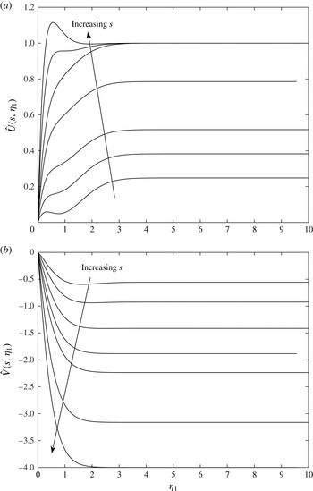
are presented in figure 2 for
 ${\it\psi}=15^{\circ }$
for a range of axial flows, increasing from
 $s=1.5$
to
 $s=16$
(corresponding to a ‘quickly’ rotating cone). We note that the
 $\hat{x}$
-component,
 $\hat{U}$
, exhibits a familiar inflectional nature, with its limiting value at the edge of the boundary layer increasing as
 $s$
increases. However, for
 $s\geqslant 5$
, we observe from the results of Kobayashi et al. (Reference Kobayashi, Kohama and Kurosawa1983) that
 ${\it\phi}=0^{\circ }$
, which is consistent with our basic flow solution where
 $\hat{U}$
recovers the streamwise basic flow component,
 $f^{\prime }$
, to within a factor of
 $s^{-1/2}$
. In contrast, the
 $y$
-component of velocity,
 $\hat{V}$
, exhibits a uniform shear and is consistently reduced as
 $s$
is increased.
Velocity profiles (a)
 $\hat{U} (s,{\it\eta}_{1})$
and (b)
 $\hat{V}(s,{\it\eta}_{1})$
in the
 $\hat{x}$
- and
 $y$
-directions, respectively, at
 ${\it\psi}=15^{\circ }$
for
 $s=1.5,2,3,4,5,10,16$
and
 ${\it\phi}=30.2^{\circ },22.5^{\circ },13.6^{\circ },6^{\circ },0^{\circ },0^{\circ },0^{\circ }$
(in the direction of the arrows).

We now outline the important link between the standard surface-normal coordinate
 ${\it\eta}$
and the modified surface-normal coordinate
 ${\it\eta}_{1}$
scaled on boundary-layer thickness according to the new velocity scales applied to the basic flow boundary-layer equations. The coordinate stretching yields
 $$\begin{eqnarray}{\it\eta}_{1}={\it\eta}\left(\frac{m+3}{2s^{1/2}}\sin {\it\psi}\right)^{1/2}.\end{eqnarray}$$
This relation enables the shifted velocity profiles
 $\tilde{U} (x,{\it\eta})$
and
 $\tilde{V}(x,{\it\eta})$
, expressed in terms of the standard boundary-layer coordinates, to be written in terms of
 $f^{\prime }(s,{\it\eta}_{1})$
and
 $g(s,{\it\eta}_{1})$
, which depend on
 $s$
and the modified boundary-layer coordinate.
We assume that the spiral waves are periodic in the
 $\hat{x}$
-direction and introduce periodicity into the perturbation quantities of vortex
 $\check{x}$
-wavenumber
 $a$
and
 $\bar{y}$
-wavenumber
 $b$
. Scaling our perturbation quantities on the boundary-layer thickness, we introduce a combined flow of the form
 $$\begin{eqnarray}\displaystyle \tilde{\boldsymbol{u}}^{\ast } & = & \displaystyle {\it\Omega}^{\ast }l^{\ast }\sin {\it\psi}\left[\{\tilde{U} (x,{\it\eta}),\tilde{V}(x,{\it\eta}),R^{-1/2}W(x,{\it\eta})\}\right.\nonumber\\ \displaystyle & & \displaystyle +\left.R^{-1/2}\{\tilde{u} ({\it\eta}),\tilde{v}({\it\eta}),\tilde{w}({\it\eta})\}\text{exp}(\text{i}a\check{x}+\text{i}b\bar{y})\right].\end{eqnarray}$$
Here
 $W(x,{\it\eta})$
is the surface-normal basic flow component, which is defined in Hussain (Reference Hussain2010) but not used explicitly in the analysis of the problem. Similarly, the pressure perturbation term scales as
 $$\begin{eqnarray}p^{\ast }=({\it\rho}^{\ast }{\it\Omega}^{\ast 2}l^{\ast 2}\sin ^{2}{\it\psi})R^{-1}\tilde{p}({\it\eta})\text{exp}(\text{i}a\check{x}+\text{i}b\bar{y}).\end{eqnarray}$$
Importantly, in order to obtain the correct form of the disturbance equations for analysing spiral vortices and circular waves (
 ${\it\phi}\neq 0^{\circ }$
and
 ${\it\phi}=0^{\circ }$
, respectively), we employ mathematical approximations, specifically using the assumption of large Reynolds number to expand the scale factors, which eventually lead to the expressions (A 6) and (A 7) in appendix A. We also focus on the large spiral wavenumber apparent within the problem, which forms the basis for a small-parameter expansion in § 4. However, a significant difference between the current approach and the analysis of Hussain et al. (Reference Hussain, Garrett and Stephen2014) is that the axial flow problem is now characterised by
 $x$
-dependence in the shifted basic flow quantities (
 $\tilde{U} (x,{\it\eta}),\tilde{V}(x,{\it\eta})$
). Hence, we may express this
 $x$
-dependence in terms of the logarithmic spiral coordinates after they have been scaled on boundary-layer thickness,
 $\check{x}$
and
 $\bar{y}$
, so that in essence
 $\tilde{U} =\tilde{U} (\check{x},\bar{y},{\it\eta})$
and
 $\tilde{V}=\tilde{V}(\check{x},\bar{y},{\it\eta})$
. This re-formulation reveals the correct length scalings that successfully model the spiral waves.
Next we proceed to investigate the orientation of the short-wavelength asymptotic structure of the centrifugal instability and hence identify the spiral wavenumber in the
 $\check{x}$
-direction as
 $a={\it\epsilon}^{-1}$
, where
 ${\it\epsilon}$
is a small parameter. Here,
 $b=O(1)$
is the corresponding wavenumber in the
 $\bar{y}$
-direction. The importance of transforming to the new logarithmic coordinate system now becomes apparent when considering that the spiral vortex wavenumbers
 $a$
and
 $b$
in the
 $\check{x}$
- and
 $\bar{y}$
-directions, respectively, enable the introduction of periodicity into the disturbance quantities. Specifically, we observe that boundary-layer growth occurs along the
 $\check{x}$
-direction, with spiral waves in the
 $\bar{y}$
-direction remaining fixed. Hence, the use of the logarithmic spiral coordinate system is not only essential to obtaining the correct length scalings upon which to model the spiral vortices of the centrifugal instability, but also to revealing the correct orientations along which these spiral vortices grow within the boundary layer. Further details of the mathematical manipulations employed in the asymptotic analysis are given in Hussain (Reference Hussain2010) and we arrive at the governing stability equations given in appendix A.
4. Asymptotic analysis
As with the asymptotic analysis presented in Hussain et al. (Reference Hussain, Garrett and Stephen2014) for the still-fluid problem, we follow a strategy of employing a large vortex wavenumber and large Reynolds number. However, given the experimental observations of Kobayashi (Reference Kobayashi1981) and Kobayashi et al. (Reference Kobayashi, Kohama and Kurosawa1983), who report the existence of both spiral and circular waves for different values of
 $s$
, we extend the analysis of Hussain et al. (Reference Hussain, Garrett and Stephen2014) to account for both zero and non-zero values of
 ${\it\phi}$
. We subsequently treat
 ${\it\phi}=0^{\circ }$
as a special case of this analysis, recovering the circular wave setup. It is important to note that the wave angle
 ${\it\phi}$
is essentially a function of both
 ${\it\psi}$
and
 $s$
, as once the half-angle and axial flow strength is determined, the instability develops accordingly, admitting spiral waves of a certain wave angle. Hence, for a fixed
 ${\it\psi}=15^{\circ }$
, we may consider
 ${\it\phi}={\it\phi}(s)$
.
We solve the governing equations to determine leading- and next-order estimates of the scaled Taylor number for neutrally stable modes, which arise due to the scaling analysis and loosely follows Hall (Reference Hall1982) for the Taylor problem of flow between concentric rotating cylinders. Importantly, we are able to make comparisons with results in the literature expressed in terms of Reynolds numbers (see § 6 for more details). The corresponding Taylor number, which characterises the relative importance of centrifugal and viscous forces, is given by
 $$\begin{eqnarray}T=\frac{2\cot {\it\psi}\cos {\it\phi}}{\sin ^{4}{\it\psi}}.\end{eqnarray}$$
In the axial flow problem, for a fixed
 ${\it\psi}$
, this quantity is an output of the analysis and represents a measure of how
 $s$
(or alternatively
 $T_{s}$
) affects the physical flow characteristics. In general, we can consider it to be a function of
 ${\it\psi}$
and parameterised by the particular
 ${\it\phi}(s)$
and
 $s$
under consideration. However, in this study, we fix
 ${\it\psi}=15^{\circ }$
and investigate the effect of varying
 $s$
. Consequently, this determines
 ${\it\phi}$
and hence the expression for
 $T$
, which is observed by Kobayashi et al. (Reference Kobayashi, Kohama and Kurosawa1983) to decrease as
 $s$
is increased for a
 $15^{\circ }$
cone. Essentially, the problem becomes a competition between the rotational flow due to the spinning cone surface and the streamwise forcing due the external oncoming axial flow. The former promotes the centrifugal instability, whereas the latter amplifies a viscous Tollmien–Schlichting instability. Hence, it is clear that the relative strengths of these two respective centrifugal and viscous mechanisms reveal why the Taylor number becomes the governing parameter in this regime. The Taylor number is closely related to the Görtler number for centrifugal instability problems and has been studied for example by Hall (Reference Hall1982) for fully developed boundary-layer flows.
Furthermore, a significant modification of the axial flow problem compared with the still-fluid case arises when considering the governing perturbation equations in appendix A. Due to the fact that the basic flow quantities and the streamwise coordinate
 $x$
depend on the logarithmic coordinates (see above in § 3), we expand the shifted basic flows in powers of
 $R^{-1/2}$
, about the location of vortex activity, namely at
 ${\it\eta}=0$
on the cone surface. This leads to the expressions
 $$\begin{eqnarray}\displaystyle \tilde{U} (\check{x},\bar{y},{\it\eta}) & = & \displaystyle R^{-1/2}{\it\eta}\frac{\partial \tilde{U} }{\partial {\it\eta}}(\check{x},\bar{y},0)+O(R^{-1}),\end{eqnarray}$$
 $$\begin{eqnarray}\displaystyle \tilde{V}(\check{x},\bar{y},{\it\eta}) & = & \displaystyle R^{-1/2}{\it\eta}\frac{\partial \tilde{V}}{\partial {\it\eta}}(\check{x},\bar{y},0)+O(R^{-1}),\end{eqnarray}$$
 $\tilde{U} (\check{x},\bar{y},0)=\tilde{V}(\check{x},\bar{y},0)=0$
. This expansion allows important quantities related to the basic flows, which appear in the governing perturbation equations, to be evaluated within the leading- and first-order asymptotic analyses.
4.1. Leading-order solution
Upon incorporating the basic flow expansions, we expand the perturbation quantities and pose a WKB solution for small values of
 ${\it\epsilon}$
, where
 $a={\it\epsilon}^{-1}$
for the wavenumber
 $a$
in the
 $\check{x}$
-direction. As for the still-fluid problem, the dominant terms in the governing equations (A 1)–(A 4) balance if we scale
 $T\sim {\it\epsilon}^{-4}$
and
 $W/V\sim O({\it\epsilon}^{-2})$
, resulting in identical perturbation expansions to those presented in Hussain et al. (Reference Hussain, Garrett and Stephen2014) (reproduced here for clarity when manipulating subsequent quantities):
 $$\begin{eqnarray}\displaystyle \tilde{u} & = & \displaystyle E(u_{0}({\it\eta})+{\it\epsilon}u_{1}({\it\eta})+{\it\epsilon}^{2}u_{2}({\it\eta})+\cdots \,),\end{eqnarray}$$
 $$\begin{eqnarray}\displaystyle \tilde{v} & = & \displaystyle {\it\epsilon}^{2}E(v_{0}({\it\eta})+{\it\epsilon}v_{1}({\it\eta})+{\it\epsilon}^{2}v_{2}({\it\eta})+\cdots \,),\end{eqnarray}$$
 $$\begin{eqnarray}\displaystyle \tilde{w} & = & \displaystyle E(w_{0}({\it\eta})+{\it\epsilon}w_{1}({\it\eta})+{\it\epsilon}^{2}w_{2}({\it\eta})+\cdots \,),\end{eqnarray}$$
 $$\begin{eqnarray}\displaystyle T & = & \displaystyle {\it\epsilon}^{-4}({\it\lambda}_{0}+{\it\lambda}_{1}{\it\epsilon}+{\it\lambda}_{2}{\it\epsilon}^{2}+\cdots \,),\end{eqnarray}$$
 ${\it\lambda}={\it\lambda}_{0}+{\it\lambda}_{1}{\it\epsilon}+{\it\lambda}_{2}{\it\epsilon}^{2}+\cdots \,,E=\text{exp}(\text{i}/{\it\epsilon})\int ^{{\it\varphi}}K({\it\tau})\,\text{d}{\it\tau}$
and
 ${\it\varphi}=(\sin {\it\psi}/\bar{h}_{1}){\it\eta}.$
However, when substituting these expansions into the governing equations to obtain the corresponding eigenrelation, we make the appropriate simplification
 $\sin ^{2}{\it\phi}\ll \cos ^{2}{\it\phi}$
in (A 1)–(A 4) relating to a small wave angle, which for
 ${\it\psi}=15^{\circ }$
holds for
 $s\geqslant 5$
and reasonably well for
 $s<5$
, from the experiments of Kobayashi et al. (Reference Kobayashi, Kohama and Kurosawa1983). This is solved to yield the scaled leading-order eigenvalue estimate
 $$\begin{eqnarray}\bar{{\it\lambda}}_{0}=-\!\left(\frac{2\sqrt{s}}{m+3}\right)^{1/2}\frac{1}{\hat{V}^{\prime }(s,0)},\end{eqnarray}$$
where the scaled eigenvalue is now given by
 $$\begin{eqnarray}\bar{{\it\lambda}}={\it\lambda}\bar{h}_{1}^{4}\frac{U_{e}}{{\it\Omega}^{\ast }l^{\ast }\sin {\it\psi}},\end{eqnarray}$$
such that
 $\bar{{\it\lambda}}=\bar{{\it\lambda}}_{0}+\bar{{\it\lambda}}_{1}{\it\epsilon}+\bar{{\it\lambda}}_{2}{\it\epsilon}^{2}+\cdots \,$
and
 $\bar{h}_{1}$
is a scale factor defined as
 $\bar{h}_{1}=1+\check{x}\cos {\it\phi}-\bar{y}\sin {\it\phi}+{\it\eta}\cos {\it\psi}\sin ^{2}{\it\phi}$
.
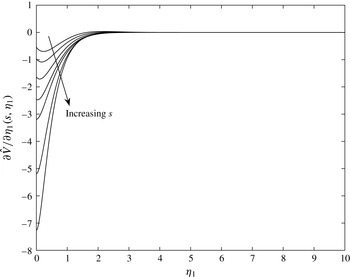
Plots of
 $(\partial \hat{V}/\partial {\it\eta}_{1})(s,{\it\eta}_{1})$
for a slender rotating cone with
 ${\it\psi}=15^{\circ },s=1.5,2,3,4,5,10,16.$

Figure 3 shows that, for
 $s\geqslant 5$
, the vortex activity is located at the wall, with the minimum of
 $\hat{V}^{\prime }(s,{\it\eta}_{1})$
at
 ${\it\eta}_{1}=0$
. However, for
 $s<5$
, the curve has a minimum slightly away from the wall, indicating that the location of vortex activity will not be at
 ${\it\eta}_{1}=0$
. This correlation is a consequence of the requirement of obtaining valid real solutions for the growth rate
 $K$
when solving the governing eigenvalue equation at leading order, which arises when following the study of Hall (Reference Hall1982) for the Taylor problem of flow between concentric rotating cylinders. For the case of
 $s<5$
, the solutions obtained are not the most dangerous modes available, but we include them as they provide useful information about non-zero wave angles (spiral waves) for a
 $15^{\circ }$
rotating cone in axial flow. Furthermore, an interesting observation pertains to the related study of Hussain et al. (Reference Hussain, Garrett and Stephen2011) on the rotating disk in axial flow, where non-stationary travelling modes become more important as the strength of oncoming axial flow increases. Specifically, for
 $s<5$
in the current problem, it appears that the location of vortex activity being slightly away from the wall suggests that travelling modes may grow as
 $T_{s}$
is increased (or
 $s$
reduced) and in fact become the most unstable modes in this parameter regime. Indeed, physically, the departure of a vortex from the wall suggests that vorticity within the boundary layer is no longer fixed on the cone surface, but is instead propagating or travelling in the effective velocity
 $\hat{x}$
-direction. Ultimately, in order to confirm whether travelling instabilities may harbour the most unstable modes for the slender-rotating-cone problem, a further investigation would be required, taking account of time-dependent terms within the governing disturbance equations (A 1)–(A 4).
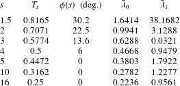
As seen from table 1, for
 ${\it\psi}=15^{\circ }$
, the scaled leading-order eigenvalue estimate
 $\bar{{\it\lambda}}_{0}$
is found to decrease as
 $s$
is increased and also increases as
 ${\it\phi}(s)$
increases for corresponding experimental observations.
Leading- and first-order eigenvalue estimates of the scaled Taylor number for rotational flow parameters
 $s$
observed by Kobayashi et al. (Reference Kobayashi, Kohama and Kurosawa1983) on a cone with
 $15^{\circ }$
half-angle.

4.2. First-order solution
We now apply Hall’s method and account for modifications to the analysis of Hussain et al. (Reference Hussain, Garrett and Stephen2014) due to the shifted basic flow terms. We also include the assumption of sufficiently small wave angle, such that
 $\tan ^{2}{\it\phi}$
is small compared with
 $1$
, which is consistent with the vortex activity being located at the wall. Hence, following Hussain et al. (Reference Hussain, Garrett and Stephen2014), we impose a thin layer of thickness
 $O({\it\epsilon}^{2/3})$
about
 ${\it\eta}_{1}=0$
, expanding the Taylor number in the form
 $$\begin{eqnarray}T={\it\epsilon}^{-4}({\it\lambda}_{0}+{\it\lambda}_{1}{\it\epsilon}^{2/3}+\cdots \,)\end{eqnarray}$$
and re-scaling the normal variable on an appropriate thickness
 ${\it\xi}={\it\varphi}/3^{1/3}{\it\epsilon}^{2/3}$
. The normal perturbation velocity is similarly expanded as
 $$\begin{eqnarray}\tilde{w}=w_{0}({\it\xi})+{\it\epsilon}^{2/3}w_{1}({\it\xi})+\cdots \,,\end{eqnarray}$$
with
 $\tilde{u} =O(1)$
and
 $\tilde{v}=O({\it\epsilon}^{2})$
as in the leading-order analysis. Substituting these expressions into the updated governing equations and equating terms of
 $O({\it\epsilon}^{2/3})$
yields a modified eigenvalue relation at first order, which is solved to give a first-order estimate of our scaled Taylor-number eigenvalue as
 $$\begin{eqnarray}\bar{{\it\lambda}}_{1}=\frac{2.3381\times 3^{1/3}}{|\hat{V}^{\prime }(s,0)|}\left(\frac{2\sqrt{s}}{m+3}\right)^{1/2}\left[\frac{\hat{V}^{\prime \prime }(s,0)+s^{-1/2}\hat{V}^{\prime }(s,0)^{2}\cos {\it\phi}}{\hat{V}^{\prime }(s,0)}\right]^{2}.\end{eqnarray}$$
The full analysis is mathematically quite detailed and provided more completely in Hussain (Reference Hussain2010). Numerical values for the first order
 $\bar{{\it\lambda}}_{1}$
are displayed in table 1 for various
 $s$
and
 ${\it\phi}$
corresponding to experimental observations.
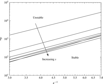
Asymptotic scaled Taylor number
 $\bar{T}$
as a function of non-dimensional vortex wavenumber
 ${\it\epsilon}^{-1}$
for
 ${\it\psi}=15^{\circ },s=1.5,2,3,4,5,10,16$
and
 ${\it\phi}(s)=30.2^{\circ },22.5^{\circ },13.6^{\circ },6^{\circ },0^{\circ },0^{\circ },0^{\circ }$
.

4.3. Asymptotic estimate of Taylor number
Finally, we combine the leading- and first-order estimates for the scaled effective Taylor number, which is given by
 $$\begin{eqnarray}\displaystyle \bar{T} & = & \displaystyle T\bar{h}_{1}^{4}\frac{U_{e}}{{\it\Omega}^{\ast }l^{\ast }\sin {\it\psi}}={\it\epsilon}^{-4}\left(\frac{2\sqrt{s}}{m+3}\right)^{1/2}\nonumber\\ \displaystyle & & \displaystyle \times ~\left[\frac{1}{\hat{V}^{\prime }(s,0)}+\frac{2.3381\times 3^{1/3}}{|\hat{V}^{\prime }(s,0)|}{\it\epsilon}^{2/3}\left(\frac{\hat{V}^{\prime \prime }(s,0)+s^{-1/2}\hat{V}^{\prime }(s,0)^{2}\cos {\it\phi}}{\hat{V}^{\prime }(s,0)}\right)^{2}+\cdots \,\right].\nonumber\\ \displaystyle & & \displaystyle\end{eqnarray}$$
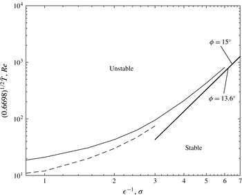
Logarithmic plots of the scaled asymptotic Taylor number against vortex wavenumber,
 ${\it\epsilon}^{-1}=a$
, are shown in figure 4 for
 ${\it\psi}=15^{\circ }$
and various values of
 $s$
. The unstable region is above the curves and the stable region below. In general, we observe that increasing
 $s$
leads to a trend of reducing the asymptotic Taylor-number branch. Physically, this can be interpreted as promoting the more dangerous centrifugal instability mode, and hence destabilising the flow, which leads to a larger unstable region above the neutral stability branch, as depicted in figure 4.
5. Numerical analysis
In this section, we develop the corresponding numerical solution, outlining the major differences between the axial flow problem formulated in § 3 and the still-fluid case presented in Hussain et al. (Reference Hussain, Garrett and Stephen2014). These arise due to the fact that the basic flow quantities
 $\tilde{U}$
and
 $\tilde{V}$
are now functions of the logarithmic spiral coordinates
 $\check{x}$
and
 $\bar{y}$
, as well as
 ${\it\eta}$
. We manipulate the disturbance equations (A 1)–(A 4) and subsequently express the basic flow terms in terms of
 ${\it\eta}_{1}$
by making use of the coordinate stretching (3.8). The analysis involves neglecting Coriolis terms and viscous streamline-curvature effects. Importantly, we note that the centrifugal mode under investigation differs from the streamline-curvature mode for large-half-angle cones (as studied in Garrett et al.
Reference Garrett, Hussain and Stephen2009), which arises due to viscous effects of the cone surface. In contrast, the centrifugal mode for small-half-angle cones arises from the centrifugal forces present in the mean flow for small
 ${\it\psi}$
, due to the effects of surface curvature. Such centrifugal curvature terms are not neglected in the analysis and contain the Taylor number as a factor. Proceeding in this fashion yields a modified Orr–Sommerfeld (OS) equation for stationary disturbances within the system, given by
 $$\begin{eqnarray}\displaystyle & & \displaystyle \left[\text{i}\left(\partial _{{\it\eta}{\it\eta}}^{2}-k^{2}\right)^{2}+\frac{Re}{\sqrt{s}}\left({\it\alpha}_{1}\hat{U} +{\it\beta}_{1}\hat{V}\right)\left(\partial _{{\it\eta}{\it\eta}}^{2}-k^{2}\right)\right.\nonumber\\ \displaystyle & & \displaystyle \quad -\left.\frac{Re}{2s}(m+3)\sin {\it\psi}\left({\it\alpha}_{1}\hat{U} ^{\prime \prime }+{\it\beta}_{1}\hat{V}^{\prime \prime }\right)\right]\tilde{w}=0,\end{eqnarray}$$
where
 $$\begin{eqnarray}{\it\alpha}_{1}=\frac{a\sin {\it\psi}}{Re},\quad {\it\beta}_{1}=b\sin {\it\psi},\quad k=\sqrt{{\it\alpha}_{1}^{2}+{\it\beta}_{1}^{2}}\end{eqnarray}$$
represent the vortex wavenumbers in the
 $\check{x}$
-,
 $\bar{y}$
- and effective velocity directions, respectively, and
 $\partial _{{\it\eta}{\it\eta}}^{2}=\partial ^{2}/\partial {\it\eta}^{2}$
. Furthermore,
 $Re=x\sin {\it\psi}$
is the local Reynolds number, interpreted as the local non-dimensional radius of the cone surface from the axis of rotation. We can relate the rotational Reynolds number, Re, to the conventional Reynolds number,
 $R$
, defined in § 3 using equation (45) of Kobayashi (Reference Kobayashi1981) to re-express the surface-curvature term, yielding
 $$\begin{eqnarray}Re=R^{1/2}\sqrt{0.6698}.\end{eqnarray}$$
In similar fashion to the still-fluid study of Hussain et al. (Reference Hussain, Garrett and Stephen2014), the system depends on the updated basic flow solutions. However, in the axial flow case, this includes a related dependence on the rotational flow parameter,
 $s$
, as well as on the wave angle
 ${\it\phi}$
, arising from the definition of the projected basic flow quantities
 $\hat{U}$
and
 $\hat{V}$
in (3.6) and (3.7). We solve the OS equation to obtain estimates of the effective vortex wavenumber
 $k$
and rotational Reynolds number
 $Re$
, for a range of values of
 $s$
and
 ${\it\phi}$
, which enable a suitable comparison with the experimental results of Kobayashi et al. (Reference Kobayashi, Kohama and Kurosawa1983).
To obtain the numerical solution, we first convert the system of disturbance equations (A 1)–(A 4) into a set of six first-order equations. Upon following the above description, specifically neglecting Coriolis and viscous streamline-curvature terms, we arrive at the fourth-order OS equation (5.1). However, we now apply an OS solver routine, which has been modified to allow existing solutions of the OS neutral curve at specific values of
 ${\it\psi}$
and (
 $s,{\it\phi}(s)$
) to be used in order to facilitate fast convergence when searching for neutral curves for the required the values. Essentially, we reduce
 ${\it\psi}$
for fixed
 $s$
, traversing from the upper branch of known neutral curves presented in Garrett et al. (Reference Garrett, Hussain and Stephen2010) for larger half-angles
 ${\it\psi}=50^{\circ }$
and
 $70^{\circ }$
. Our current basic flows are used as input solutions to the OS solver in order to obtain results for
 ${\it\psi}=15^{\circ }$
. Subsequently we repeat the updated routine by now reducing
 $s$
for fixed
 ${\it\psi}=15^{\circ }$
, traversing from the known upper branch for large
 $s$
(
 $s\rightarrow \infty$
) and reducing to the required parameter range of
 $s$
investigated by Kobayashi et al. (Reference Kobayashi, Kohama and Kurosawa1983). We again use the shifted basic flow solutions for varying (
 $s,{\it\phi}(s)$
) at
 ${\it\psi}=15^{\circ }$
. The result is that the modified OS solver enables us to gradually merge, in an incremental process, from previously computed OS solutions in order to obtain the OS neutral stability curves that we seek for the required values of
 ${\it\psi}$
and (
 $s,{\it\phi}(s)$
).
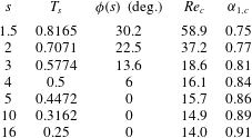
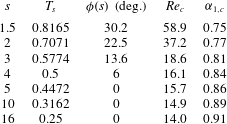
We present numerical predictions of the critical Reynolds numbers and critical vortex wavenumbers for
 ${\it\psi}=15^{\circ }$
in a range of axial flows varying from
 $s=1.5$
to
 $s=16$
in table 2. The results show that an increase in
 $s$
leads to a reduction in the critical Reynolds number, which suggests that a stronger rotational flow promotes the centrifugal instability mode, hence destabilising the flow. This is supported by the critical vortex wavenumbers in the effective velocity direction, which increase as
 $s$
is increased, leading to greater amplification rates for steady flow. Importantly, we observe close agreement with the experimental observations of Kobayashi et al. (Reference Kobayashi, Kohama and Kurosawa1983) and with our asymptotic results in § 4, discussion of which is developed below in § 6.
Numerical calculations of the critical Reynolds numbers,
 $Re_{c}$
, and critical vortex wavenumbers,
 ${\it\alpha}_{1,c}$
, in the effective velocity direction for a cone of
 $15^{\circ }$
half-angle in a range of axial flows defined by
 $s$
, with corresponding vortex wave angles,
 ${\it\phi}$
.
However, at this stage we must note that the OS numerical analysis presented neglects Coriolis and streamline-curvature effects. These effects are known to yield a characteristic two-lobe structure for the neutral-stability curve, which cannot be captured by the OS analysis. This behaviour is concentrated around the critical Reynolds number region of the stability curve. Consequently, the results of the OS numerical analysis will exhibit a slight discrepancy when compared with the experimental measurements of Kobayashi et al. (Reference Kobayashi, Kohama and Kurosawa1983) around the critical Reynolds number region.
First, we justify the use of the OS numerical stability analysis, as it represents a useful simplification of the disturbance equations (A 1)–(A 4). Nevertheless, the process of obtaining the numerical solution is complicated by the use of the modified OS solver routine, which requires the updated basic flow solutions for successively varying values of
 ${\it\psi}$
and subsequently (
 $s,{\it\phi}(s)$
) in order to converge gradually to an updated neutral curve for
 ${\it\psi}=15^{\circ }$
and the relevant axial flow strengths. While the process is incremental and time-consuming when compared with, for example, the asymptotic solution presented in § 4, it improves in accuracy, yielding closer comparisons with the experimental measurements of Kobayashi et al. (Reference Kobayashi, Kohama and Kurosawa1983) as
 $Re$
increases.
Secondly, the current OS numerical solution represents an interesting comparison with the numerical method of Kobayashi (Reference Kobayashi1981) and Kobayashi et al. (Reference Kobayashi, Kohama and Kurosawa1983), revealing the effect of perturbing around the more accurate base flows
 $\hat{U}$
and
 $\hat{V}$
used in this study. As the majority of the terms in the OS analysis leading to (5.1) depend on these base flow quantities, improving their accuracy can significantly boost the overall accuracy of the OS neutral-curve solution. In fact, we observe that the numerical analysis presented yields generally better agreement with the experimental data of Kobayashi et al. (Reference Kobayashi, Kohama and Kurosawa1983) than the numerical calculations. As such, these comparisons are expanded upon and discussed later in § 6.
Lastly, we note that in the numerical analysis,
 ${\it\phi}(s)$
is treated as a general unknown value. Neutral stability curves are constructed for
 ${\it\psi}=15^{\circ }$
and the required values of
 $s$
. As in Kobayashi (Reference Kobayashi1981), a range of
 ${\it\phi}$
values are investigated around the critical Reynolds number region, in order to ascertain the
 ${\it\phi}$
with the minimum critical Reynolds number. These values of
 ${\it\phi}$
exist in a range, for example for
 ${\it\psi}=15^{\circ }$
and
 $s=3$
,
 ${\it\phi}$
lies between
 $5^{\circ }$
and
 $20^{\circ }$
. The
 ${\it\phi}$
values presented in this study are selected to enable direct comparisons between our numerical analysis and the numerical results of Kobayashi (Reference Kobayashi1981) and Kobayashi et al. (Reference Kobayashi, Kohama and Kurosawa1983), showing the improved accuracy in our basic flows and perturbation solutions compared with their numerical techniques. Furthermore, if we consider figure 10 in Kobayashi et al. (Reference Kobayashi, Kohama and Kurosawa1983), we see that there is a wide range of experimental data measurements available for
 ${\it\phi}$
. Our numerical results can be compared with these, but have not been chosen to fit this data.
6. Comparison between asymptotic and numerical analysis
In this section, we compare the numerical OS neutral stability curves with the large-vortex-wavenumber asymptotic predictions. We use modified scalings linking the Taylor number defined in (4.1) to the rotational Reynolds number (used in Kobayashi et al. Reference Kobayashi, Kohama and Kurosawa1983), which yields
 $$\begin{eqnarray}Re=\bar{T}\sqrt{0.6698}\end{eqnarray}$$
for large Reynolds number,
 $Re$
, and large Taylor number,
 $T$
.
We again compare scaled effective asymptotic Taylor number,
 $\bar{T}$
, versus large vortex wavenumber,
 ${\it\epsilon}^{-1}$
, and the numerical OS neutral curves of Reynolds number,
 $Re$
, versus vortex wavenumber
 ${\it\sigma}$
in the effective velocity direction. Here,
 ${\it\sigma}={\it\alpha}{\it\delta}_{1}/h_{1}$
, from Kobayashi (Reference Kobayashi1981), where
 ${\it\alpha}$
represents the wavenumber in the effective velocity direction. Following comparisons with the definitions used in Kobayashi (Reference Kobayashi1981), we associate
 ${\it\sigma}$
with our vortex wavenumber in the
 $\check{x}$
-direction,
 ${\it\alpha}_{1}$
, given in the OS equation (5.1).
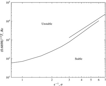
A comparison between the scaled effective asymptotic Taylor number
 $\bar{T}$
(upper line) and the Reynolds number
 $Re$
predicted by the Orr–Sommerfeld analysis (lower line), against vortex wavenumbers
 ${\it\epsilon}^{-1}$
and
 ${\it\sigma}$
respectively, for
 ${\it\psi}=15^{\circ },s=1.5$
.

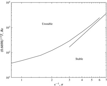
A comparison between the scaled effective asymptotic Taylor number
 $\bar{T}$
(lower line) and the Reynolds number
 $Re$
predicted by the Orr–Sommerfeld analysis (upper line), against vortex wavenumbers
 ${\it\epsilon}^{-1}$
and
 ${\it\sigma}$
respectively, for
 ${\it\psi}=15^{\circ },s=2$
.

A comparison between the scaled effective asymptotic Taylor numbers
 $\bar{T}$
(lower solid lines) for
 ${\it\phi}=13.6^{\circ },15^{\circ }$
and the Reynolds number
 $Re$
predicted by the Orr–Sommerfeld analysis (upper solid line) as well as by the numerical calculations of Kobayashi (Reference Kobayashi1981) (dashed curve), plotted against vortex wavenumbers
 ${\it\epsilon}^{-1}$
and
 ${\it\sigma}$
respectively, for
 ${\it\psi}=15^{\circ },s=3$
. Note that the asymptotic estimates for
 ${\it\phi}=13.6^{\circ }$
and
 ${\it\phi}=15^{\circ }$
appear very close together, with
 ${\it\phi}=15^{\circ }$
slightly above
 ${\it\phi}=13.6^{\circ }$
.

Figures 5–7 show log–log comparisons between the scaled effective asymptotic Taylor number,
 $\bar{T}$
, expanded in terms of vortex wavenumber
 ${\it\epsilon}^{-1}$
, versus the numerically predicted Reynolds number
 $Re$
, expressed in terms of
 ${\it\sigma}$
, for
 ${\it\psi}=15^{\circ }$
and
 $s=1.5,2$
and
 $3$
, respectively. In each figure, we compute asymptotic curves for the corresponding wave angles used in the experiments of Kobayashi et al. (Reference Kobayashi, Kohama and Kurosawa1983), namely
 ${\it\phi}=30.2^{\circ },22.5^{\circ }$
and
 $13.6^{\circ }$
respectively. Additionally, we also present asymptotic curves for
 ${\it\phi}=15^{\circ }$
in the case of
 $s=3$
in figure 7, which corresponds to the wave angle used in the numerical study of Kobayashi (Reference Kobayashi1981).
For
 ${\it\psi}=15^{\circ }$
, we observe good qualitative agreement between the OS neutral curves and the asymptotic branches of the scaled effective Taylor number for
 $s=1.5,2$
and
 $3$
. In particular, the agreement between the asymptotics and numerics becomes better for larger values of
 $\bar{T}$
, further along the asymptotic branch. Due to the nature of the large vortex wavenumbers and large Reynolds numbers used in the asymptotic analysis, we expect better agreement for large values of
 ${\it\epsilon}^{-1}$
and
 ${\it\sigma}$
. Furthermore, the accuracy of the OS numerical neutral curves should increase for larger values of
 $Re$
, which is consistent with our observations as we move along the upper branch of the neutral stability curves.
Furthermore, as
 $s$
increases, we observe closer general agreement between the asymptotic and numerical estimates, which can be seen as we move from figures 5 to 7. One explanation pertains to a modelling assumption used in § 4 to derive the asymptotic Taylor number estimates, which requires a sufficiently small wave angle. This is consistent with the vortex activity being located at the wall, which is the case for
 $s\geqslant 5$
. For smaller values of
 $s$
, this location departs slightly from the wall, as can be seen in figure 3. The consequence is that the asymptotic stability modes obtained, whilst not being the most dangerous modes available, will nevertheless be close to the most dangerous modes. Hence, comparisons between the asymptotic and numerical estimates should yield greater accuracy for larger values of
 $s$
, where the asymptotic stability modes are closer to the neutral stability modes obtained from the numerical analysis.
A second explanation for the closer agreement between the asymptotics and numerics for larger values of
 $s$
relates to a physical interpretation of the problem, where a larger value of
 $s$
corresponds to a stronger rotational flow component. This essentially promotes the centrifugal instability, which has been used to model the important length scalings for both the asymptotic and numerical analyses. Hence, the parameter regime of large
 $s$
(or small
 $T_{s}$
) corresponds to the closest theoretical model of the counter-rotating vortex activity observed for slender rotating cones in axial flow. In contrast, smaller values of
 $s$
lead to a stronger streamwise flow component. This instead promotes a distinct viscous Tollmien–Schlichting instability, which forces the spiral waves further along in the streamwise direction. Overall, the centrifugal instability is identified as the more dangerous mechanism, with a stronger streamwise flow component acting to stabilise the flow versus the destabilising rotational flow component. Consequently, larger values of
 $s$
should yield closer agreement between the asymptotic and numerics, as observed.
In the specific case of figure 7, we observe that both our numerical OS results (solid curve) and the numerical calculations of Kobayashi (Reference Kobayashi1981) (dashed curve) lead to slightly closer agreement with the asymptotic branch for
 ${\it\phi}=15^{\circ }$
rather than for
 ${\it\phi}=13.6^{\circ }$
. This is consistent with the fact that
 ${\it\phi}=15^{\circ }$
corresponds to Kobayashi’s numerical study, whereas
 ${\it\phi}=13.6^{\circ }$
relates to the experiments of Kobayashi et al. (Reference Kobayashi, Kohama and Kurosawa1983).
More importantly, figure 7 shows that while both our numerical results (solid curve) and those of Kobayashi (Reference Kobayashi1981) (dashed curve) agree well with the asymptotic branches for large
 ${\it\sigma}$
and large
 $Re$
, our OS calculations predict a higher critical Reynolds number at the leading edge of the curve, compared with the numerical results of Kobayashi (Reference Kobayashi1981). This discrepancy is discussed further in § 7, where we compare both predictions for the critical Reynolds numbers, with the experimental observations of Kobayashi et al. (Reference Kobayashi, Kohama and Kurosawa1983), showing our results are closer to their experimental measurements, as depicted in figure 9 below.
One explanation for the observed improvement in our results involves considering the differences between our numerical analysis and that of Kobayashi (Reference Kobayashi1981). As discussed earlier in § 2, Kobayashi’s basic flows appear to show some deviation from the required convergent behaviour at the edge of the boundary layer, matching with the inviscid potential flow solution
 $U_{e}$
. In contrast, our shifted basic flows developed in § 3 and obtained using the commercial NAG routine D03PEF exhibit strongly convergent behaviour at the edge of the boundary layer (as shown in figure 2). While in the asymptotic model many of the important quantities which feed into the analysis are calculated at the wall location (
 ${\it\eta}=0$
), this is not the case for the numerical model. Specifically, we see from the governing OS stability equation (5.1) that the complete basic flow profiles are fed into the numerical analysis when employing the modified OS solver described in § 5. Hence, greater accuracy in the calculation of these shifted basic flows is important for the numerical model to ensure more accurate predictions of the OS neutral curves when compared with those curves of Kobayashi (Reference Kobayashi1981), particularly near the regions corresponding to the critical values of the rotational Reynolds number
 $Re$
.
7. Conclusion
In this paper, we have presented a physical extension to the problem of boundary-layer flow over a rotating cone. Specifically, by imposing an oncoming axial flow, we have developed distinct asymptotic and numerical analyses based on the centrifugal-instability mode, which captures the effects of surface curvature and incorporates the rotational flow component. Furthermore, through the control parameter
 $s$
, we have also included the effects of the streamwise flow component, which is susceptible to a viscous Tollmien–Schlichting instability. We observe that the combined flow is a competition between these two competing instabilities, with the former the most dangerous mechanism. Meanwhile, the latter acts to stabilise the flow and force the counter-rotating spiral waves along the cone surface in the streamwise direction.
In general, we observe close agreement between our asymptotic and OS numerical stability results. We also obtain reasonably good comparisons between our numerics and the numerical stability calculations of Kobayashi (Reference Kobayashi1981) in figure 7. Importantly, while we have used the asymptotic results to provide an envelope for the right-hand branch of the numerical neutral stability curve, they are unable to predict the effect of varying axial flow on the critical Reynolds numbers. Nevertheless, the asymptotic analysis has proved invaluable in this study, as it reveals the correct length scalings on which to model the counter-rotating vortex pairs, which characterise the centrifugal mode. Furthermore, by expanding the shifted basic flows about the location
 ${\it\eta}=0$
, we were able to confirm that the vortex activity of the most dangerous modes is located at the wall. Subsequently, as
 $s$
was varied, we tracked the location of vortex activity, observing that it departs slightly from the wall for
 $s<5$
. As a result, we have posed the hypothesis that stationary modes could dominate in the region
 $s\geqslant 5$
, but below this non-stationary (or ‘travelling’) modes may begin to grow. Such an observation requires further investigation, but would not be possible solely through a numerical analysis. Hence, the importance of an asymptotic analysis is clear in revealing the underlying physical mechanisms at work, along with how they might interact.
In contrast, the OS numerical stability results complement the asymptotics in confirming the existence of the neutral stability curve for the centrifugal mode. Furthermore, we observe a reduction in the critical Reynolds number
 $Re_{c}$
as well as an increase in the critical amplification rate
 ${\it\alpha}_{1,c}$
with increasing
 $s$
, suggesting that larger values of
 $s$
are destabilising (or larger values of
 $T_{s}$
are stabilising), as seen in table 2. Hence, the centrifugal-instability mode is physically the most dangerous mechanism, despite alternatives being present, including the cross-flow and Tollmien–Schlichting instabilities.
Finally, we propose that a condition of ‘optimal’ stability exists around
 $s=T_{s}=1$
, where the competing effects of the rotational and streamwise flow components balance. For
 $s<1$
(or
 $T_{s}>1$
), the physical problem changes from a ‘quickly’ rotating cone (the parameter range considered in this study) to a ‘slowly’ rotating cone. In this latter regime, the physical effect of the oncoming axial flow strengthens, thereby promoting the streamwise Tollmien–Schlichting instability, which begins to dominate over the centrifugal mode. This conclusion has interesting implications for the design of spinning projectiles, for example in military and defence applications. Here, the streamwise component is often large due to the projected velocity of the missile. For example, projectile applications that involve high rotation rates, such as spinning bullets and spinning missiles, can spin up to
 $3000^{\circ }\,\text{s}^{-1}$
and higher. In such a case, it is important to design a missile that spins at sufficiently high rotation rate in order to promote the centrifugal mode and obtain a suitable balance between the competing instabilities. In fact, the primary instability can break down to a secondary instability, which has been observed, for example, by Kohama (Reference Kohama1985) in the formation of ‘horseshoe-like’ vortices. Essentially, the aim in such spinning body applications is to reduce the parameter scope for transition to turbulence within the flow. Therefore, influencing the primary and, potentially, the secondary instability along the spinning body over a longer streamwise distance may achieve a delay in turbulent transition, which consequently leads to more accurate targeting and projectile control properties. It should be noted at this point that the current study neglects the effects of compressibility, which would play a significant role in accurately modelling such high-speed applications. In the light of this, the authors are presently working on a compressible flow study of the rotating cone (Towers & Garrett Reference Towers and Garrett2014) and hope to report on this in the near future.
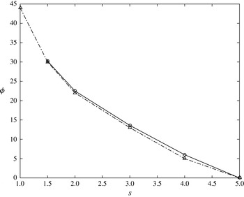
Figure 8 presents the observed wave angle,
 ${\it\phi}$
, versus various
 $s$
for a
 $15^{\circ }$
rotating cone. We compare results from the present study with the experiments of Kobayashi et al. (Reference Kobayashi, Kohama and Kurosawa1983), observing close agreement. Both studies show that in the regime of a ‘quickly’ rotating cone (
 $s>1$
), increasing
 $s$
leads to a reduction in
 ${\it\phi}$
, to the point where
 ${\it\phi}=0$
for
 $s\geqslant 5$
, physically corresponding to the transition from spiral waves to circular or ‘Taylor’ vortices. Interestingly, this appears consistent with the asymptotic analysis in § 4 where, for
 $s\geqslant 5$
, the vortex activity remains located on the wall at
 ${\it\eta}=0$
. Conversely for
 $s<5$
, the stronger axial flow (larger
 $T_{s}$
) acts to sweep vorticity in the streamwise direction, which is again consistent with the asymptotic findings in § 4, namely that the vortex activity undergoes a slight departure from the wall in this regime.
We note that
 ${\it\phi}={\it\phi}(s)$
forms a pseudo-parameter in the numerical analysis. For
 ${\it\psi}=15^{\circ }$
and fixed
 $s$
, we obtained basic flows for a range of
 ${\it\phi}$
, supplying these as input profiles to the modified OS solver discussed in § 5 in order to construct the neutral stability curves from the corresponding curves for larger cone half-angles. Consequently, following the method of Kobayashi (Reference Kobayashi1981), the values of
 ${\it\phi}$
yielding the lowest critical Reynolds numbers when plotting the stability curves were chosen to identify the most unstable modes and compare with the experimental measurements of Kobayashi et al. (Reference Kobayashi, Kohama and Kurosawa1983). Additionally, we observe more consistent and smoother convergence behaviour in the OS solver for these
 ${\it\phi}$
, suggesting that the numerical analysis accurately captures the dominant centrifugal mode within the parameter range for the
 $s$
under investigation.
A comparison between the experimental observations of Kobayashi et al. (Reference Kobayashi, Kohama and Kurosawa1983) (dot-dashed line, ▵) and the current theoretical predictions (solid line, ○) of the vortex orientation angle,
 ${\it\phi}$
, at the onset of instability. The diagram illustrates that
 ${\it\phi}(s)$
reduces with increased rotational flow parameter,
 $s$
, to a limiting value of
 ${\it\phi}=0^{\circ }$
at
 $s=5$
.

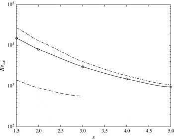
A comparison between the experimental and numerical observations of Kobayashi et al. (Reference Kobayashi, Kohama and Kurosawa1983) (dot-dashed and dashed curves, respectively) and the current theoretical predictions (solid curve, ○) of the critical Reynolds number,
 $Re_{x,c}$
, at the onset of instability. The diagram illustrates that
 $Re_{x,c}$
reduces with increased rotational flow parameter,
 $s$
.

In figure 9, we present a logarithmic plot of the critical experimental Reynolds number
 $Re_{x,c}$
against various values of
 $s$
for a cone with
 ${\it\psi}=15^{\circ }$
. We compare our numerics with both the numerical and experimental results in figure 6 of Kobayashi et al. (Reference Kobayashi, Kohama and Kurosawa1983), using (5.3) and identifying
 $R$
at the critical location to be
 $Re_{x,c}$
in Kobayashi’s notation. Similar to table 2, we observe a reduction in
 $Re_{x,c}$
as
 $s$
is increased, suggesting that increasing the rotational flow is destabilising. In general, we observe good comparisons with the experimental measurements of Kobayashi et al. (Reference Kobayashi, Kohama and Kurosawa1983), with improving accuracy as
 $s$
is increased. One explanation for this is that the centrifugal mechanism strengthens for increasing
 $s$
, due to the larger rotational flow component. Hence, the length scalings and approximations governing the numerical analysis will yield better comparisons with experiments as
 $s$
increases.
Interestingly, while our results appear to under-predict the critical Reynolds number
 $Re_{x,c}$
, we observe closer agreement with the experiments of Kobayashi et al. (Reference Kobayashi, Kohama and Kurosawa1983) than their numerical results. This may be due to the increased accuracy achieved in calculating the shifted basic flow profiles. Indeed, for the numerical analysis in § 5, we use the complete shifted basic flow profiles, as opposed to the asymptotic analysis in § 4, where predominantly the quantities at
 ${\it\eta}=0$
are utilised. Specifically, use of the commercial NAG routine D03PEF appears to yield more accurate basic flows, with smoother convergence behaviour at the edge of the boundary layer, compared with those obtained in Kobayashi (Reference Kobayashi1981). As a result, this increased accuracy is transferred to the numerical stability analysis, where the basic flows are used in solving the governing OS equation (5.1). Ultimately, this leads to more accurate predictions of the critical
 $Re_{x,c}$
, when compared with the experiments of Kobayashi et al. (Reference Kobayashi, Kohama and Kurosawa1983). Furthermore, we notice our results are consistent with the related study of Garrett et al. (Reference Garrett, Hussain and Stephen2010), where the OS neutral curves for a broad rotating cone (
 ${\it\psi}=70^{\circ }$
) under-predict the critical Reynolds number, compared with the corresponding neutral curves obtained from the full perturbation system.
The problem of experimentally investigating spinning body applications with an axial flow introduced remains an open question. This is predominantly due to the inherent difficulties in accurate measurement of the important aerodynamic parameters when incorporating an external oncoming axial flow. Consequently, theoretical studies, such as the asymptotic and numerical analyses presented here, represent important pathways to progress in such complex problems, which often involve the interaction of a number competing instabilities.
While the present study uses an OS numerical analysis to estimate the neutral stability curves, it cannot accurately model the familiar two-lobed structure of the curve near the critical Reynolds number region. However, the numerics yield results of improving accuracy as
 $Re$
increases, and also recover the asymptotics for large
 $Re$
and
 ${\it\sigma}$
, which utilise the full disturbance equations. Furthermore, comparisons of our OS results for
 $Re_{x,c}$
with the experiments of Kobayashi et al. (Reference Kobayashi, Kohama and Kurosawa1983) in figure 9 show reasonably good agreement. Nevertheless, we propose a numerical analysis of the full perturbation equations, including the Coriolis and viscous streamline-curvature effects, as an extension to this problem. It should be stressed that, as in § 5, such an analysis will obtain neutral curves for the required values of
 ${\it\psi}$
and
 $s$
. We will subsequently investigate the stability curves for the range of
 ${\it\phi}$
which produces the lowest critical Reynolds numbers. This will form an accurate estimate for
 ${\it\phi}$
that can be compared to existing experimental and numerical results. Ultimately, utilisation of the updated basic flows presented in this study would potentially lead to closer comparison with existing experiments, not to mention with any potential future experimental studies. In the light of this, we are currently in the process of developing and extending the work of Garrett et al. (Reference Garrett, Hussain and Stephen2009) to a broad rotating cone undergoing a cross-flow instability, to incorporate an oncoming axial flow. We hope to extend these results in due course to the current problem of a slender rotating cone in axial flow.
Acknowledgements
Z.H. wishes to acknowledge Manchester Metropolitan University and the University of Leicester, where some of the results for this paper were obtained. The authors are also grateful to the referees for their useful comments regarding the structure of a previous version of the article, and drawing our attention to comparisons with results from Kobayashi (Reference Kobayashi1981), Kobayashi et al. (Reference Kobayashi, Kohama and Kurosawa1983).
Appendix A. The governing perturbation equations
 $$\begin{eqnarray}\displaystyle & & \displaystyle \displaystyle \text{i}a\frac{\sin {\it\psi}}{\bar{h}_{1}}\tilde{u} +\frac{\sin {\it\psi}(\tilde{u} \cos {\it\phi}+\tilde{v}\sin {\it\phi})}{\bar{h}_{1}\bar{h}_{2}}+\text{i}b\frac{\sin {\it\psi}}{\bar{h}_{2}}\tilde{v}+\frac{\partial \tilde{w}}{\partial {\it\eta}}\nonumber\\ \displaystyle & & \displaystyle \displaystyle \quad +\,\left(\frac{\cos {\it\psi}\cos ^{2}{\it\phi}}{\bar{h}_{2}}+\frac{\cos {\it\psi}\sin ^{2}{\it\phi}}{\bar{h}_{1}}\right)\tilde{w}=0,\end{eqnarray}$$
 $$\begin{eqnarray}\displaystyle & & \displaystyle \displaystyle \left(\text{i}a\frac{\sin {\it\psi}}{\bar{h}_{1}}\tilde{U} (\check{x},\bar{y},{\it\eta})+\text{i}b\frac{\sin {\it\psi}}{\bar{h}_{2}}\tilde{V}(\check{x},\bar{y},{\it\eta})+W\frac{\partial }{\partial {\it\eta}}\right)\tilde{u} \nonumber\\ \displaystyle & & \displaystyle \displaystyle \quad +\,\frac{\sin {\it\psi}}{\bar{h}_{1}}\frac{\partial \tilde{U} }{\partial \check{x}}(\check{x},\bar{y},{\it\eta})\tilde{u} -\frac{\sin {\it\psi}}{\bar{h}_{2}}\frac{\partial \tilde{U} }{\partial \bar{y}}(\check{x},\bar{y},{\it\eta})\tilde{v}+\frac{\partial \tilde{U} }{\partial {\it\eta}}(\check{x},\bar{y},{\it\eta})\tilde{w}\nonumber\\ \displaystyle & & \displaystyle \displaystyle \quad +\,\frac{\sin {\it\psi}}{\bar{h}_{1}\bar{h}_{2}}[\tilde{U} (\check{x},\bar{y},{\it\eta})\tilde{v}+\tilde{V}(\check{x},\bar{y},{\it\eta})\tilde{u} ]\sin {\it\phi}+\left(\tilde{U} (\check{x},\bar{y},{\it\eta})\tilde{w}+W\tilde{u} \right)\frac{\cos {\it\psi}}{\bar{h}_{1}}\sin ^{2}{\it\phi}\nonumber\\ \displaystyle & & \displaystyle \displaystyle \quad -\,2\frac{\sin {\it\psi}}{\bar{h}_{1}\bar{h}_{2}}\tilde{V}(\check{x},\bar{y},{\it\eta})\tilde{v}\cos {\it\phi}-2(\tilde{w}\cot {\it\psi}\sin {\it\phi}+\tilde{v})\nonumber\\ \displaystyle & & \displaystyle \displaystyle =-\text{i}a\frac{\sin {\it\psi}}{\bar{h}_{1}}\tilde{p}+\bar{{\rm\nabla}}^{2}\tilde{u} +\left[\frac{\partial }{\partial \check{x}}\left(\frac{1}{\bar{h}_{1}\bar{h}_{2}}\frac{\partial (\bar{h}_{1}\bar{h}_{2})}{\partial \check{x}}\right)\tilde{u} -2\text{i}b\frac{\sin {\it\psi}}{\bar{h}_{2}^{2}}\frac{\partial \bar{h}_{2}}{\partial \check{x}}\tilde{v}\right.\nonumber\\ \displaystyle & & \displaystyle \displaystyle \quad -\,\left.\left(\frac{\sin {\it\psi}}{\bar{h}_{2}^{3}}\frac{\partial \bar{h}_{2}}{\partial \bar{y}}\frac{\partial \bar{h}_{2}}{\partial \check{x}}+\frac{\sin {\it\psi}}{\bar{h}_{1}^{2}\bar{h}_{2}}\frac{\partial \bar{h}_{1}}{\partial \bar{y}}\frac{\partial \bar{h}_{1}}{\partial \check{x}}\right)\tilde{v}-\left(\frac{\sin {\it\psi}}{\bar{h}_{1}^{3}}\frac{\partial \bar{h}_{1}}{\partial {\it\eta}}\frac{\partial \bar{h}_{1}}{\partial \check{x}}+\frac{\sin {\it\psi}}{\bar{h}_{1}\bar{h}_{2}^{2}}\frac{\partial \bar{h}_{2}}{\partial {\it\eta}}\frac{\partial \bar{h}_{2}}{\partial \check{x}}\right)\tilde{w}\right],\nonumber\\ \displaystyle & & \displaystyle\end{eqnarray}$$
 $$\begin{eqnarray}\displaystyle & & \displaystyle \displaystyle \left(\text{i}a\frac{\sin {\it\psi}}{\bar{h}_{1}}\tilde{U} (\check{x},\bar{y},{\it\eta})+\text{i}b\frac{\sin {\it\psi}}{\bar{h}_{2}}\tilde{V}(\check{x},\bar{y},{\it\eta})+W\frac{\partial }{\partial {\it\eta}}\right)\tilde{v}\nonumber\\ \displaystyle & & \displaystyle \displaystyle \quad +\,\frac{\sin {\it\psi}}{\bar{h}_{1}}\frac{\partial \tilde{V}}{\partial \check{x}}(\check{x},\bar{y},{\it\eta})\tilde{u} -\frac{\sin {\it\psi}}{\bar{h}_{2}}\frac{\partial \tilde{V}}{\partial \bar{y}}(\check{x},\bar{y},{\it\eta})\tilde{v}+\frac{\partial \tilde{V}}{\partial {\it\eta}}(\check{x},\bar{y},{\it\eta})\tilde{w}\nonumber\\ \displaystyle & & \displaystyle \displaystyle \quad +\,\frac{\sin {\it\psi}}{\bar{h}_{1}\bar{h}_{2}}[\tilde{U} (\check{x},\bar{y},{\it\eta})\tilde{v}+\tilde{V}(\check{x},\bar{y},{\it\eta})\tilde{u} ]\cos {\it\phi}+\left(\tilde{V}(\check{x},\bar{y},{\it\eta})\tilde{w}+W\tilde{v}\right)\frac{\cos {\it\psi}}{\bar{h}_{2}}\cos ^{2}{\it\phi}\nonumber\\ \displaystyle & & \displaystyle \displaystyle \quad -\,2\frac{\sin {\it\psi}}{\bar{h}_{1}\bar{h}_{2}}\tilde{U} (\check{x},\bar{y},{\it\eta})\tilde{u} \sin {\it\phi}+2(\tilde{w}\cot {\it\psi}\cos {\it\phi}+\tilde{u} )\nonumber\\ \displaystyle & & \displaystyle \displaystyle =-\text{i}b\frac{\sin {\it\psi}}{\bar{h}_{2}}\tilde{p}+\bar{{\rm\nabla}}^{2}\tilde{v}+\left[\left(\frac{\sin {\it\psi}}{\bar{h}_{2}^{3}}\frac{\partial \bar{h}_{2}}{\partial \check{x}}\frac{\partial \bar{h}_{2}}{\partial \bar{y}}+\frac{\sin {\it\psi}}{\bar{h}_{1}^{2}\bar{h}_{2}}\frac{\partial \bar{h}_{1}}{\partial \check{x}}\frac{\partial \bar{h}_{1}}{\partial \bar{y}}\right)\tilde{u} \right.\nonumber\\ \displaystyle & & \displaystyle \displaystyle \quad +\,\frac{\sin ^{2}{\it\psi}}{\bar{h}_{2}^{2}}\tilde{v}-2\text{i}b\frac{\sin {\it\psi}}{\bar{h}_{2}^{2}}\left(\frac{\partial \bar{h}_{2}}{\partial \check{x}}\tilde{u} +\frac{\partial \bar{h}_{2}}{\partial {\it\eta}}\tilde{w}\right)\!-\!\left.\left(\frac{\sin {\it\psi}}{\bar{h}_{1}^{3}}\frac{\partial \bar{h}_{1}}{\partial {\it\eta}}\frac{\partial \bar{h}_{1}}{\partial \bar{y}}+\frac{\sin {\it\psi}}{\bar{h}_{1}\bar{h}_{2}^{2}}\frac{\partial \bar{h}_{2}}{\partial {\it\eta}}\frac{\partial \bar{h}_{2}}{\partial \bar{y}}\right)\tilde{w}\right],\nonumber\\ \displaystyle & & \displaystyle\end{eqnarray}$$
 $$\begin{eqnarray}\displaystyle & & \displaystyle \displaystyle \left(\text{i}a\frac{\sin {\it\psi}}{\bar{h}_{1}}\tilde{U} (\check{x},\bar{y},{\it\eta})+\text{i}b\frac{\sin {\it\psi}}{\bar{h}_{2}}\tilde{V}(\check{x},\bar{y},{\it\eta})+W\frac{\partial }{\partial {\it\eta}}\right)\tilde{w}+\frac{\partial W}{\partial {\it\eta}}\tilde{w}\nonumber\\ \displaystyle & & \displaystyle \displaystyle \quad -\,2\frac{\cos {\it\psi}\sin ^{2}{\it\phi}}{\bar{h}_{1}}\tilde{U} (\check{x},\bar{y},{\it\eta})\tilde{u} -2\frac{\cos {\it\psi}\cos ^{2}{\it\phi}}{\bar{h}_{2}}\tilde{V}(\check{x},\bar{y},{\it\eta})\tilde{v}\nonumber\\ \displaystyle & & \displaystyle \displaystyle \quad -\,2(\tilde{v}\cot {\it\psi}\cos {\it\phi}-\tilde{u} \cot {\it\psi}\sin {\it\phi})=-\frac{\partial \tilde{p}}{\partial {\it\eta}}+\bar{{\rm\nabla}}^{2}\tilde{w}\nonumber\\ \displaystyle & & \displaystyle \displaystyle \quad -\,\left(\frac{\sin {\it\psi}}{\bar{h}_{1}^{3}}\frac{\partial \bar{h}_{1}}{\partial \check{x}}\frac{\partial \bar{h}_{1}}{\partial {\it\eta}}+\frac{\sin {\it\psi}}{\bar{h}_{1}\bar{h}_{2}^{2}}\frac{\partial \bar{h}_{2}}{\partial \check{x}}\frac{\partial \bar{h}_{2}}{\partial {\it\eta}}\right)\tilde{u} +\left(\frac{\sin {\it\psi}}{\bar{h}_{2}^{3}}\frac{\partial \bar{h}_{2}}{\partial \bar{y}}\frac{\partial \bar{h}_{2}}{\partial {\it\eta}}+\frac{\sin {\it\psi}}{\bar{h}_{1}^{2}\bar{h}_{2}}\frac{\partial \bar{h}_{1}}{\partial \bar{y}}\frac{\partial \bar{h}_{1}}{\partial {\it\eta}}\right)\tilde{v}\nonumber\\ \displaystyle & & \displaystyle \displaystyle \quad +\,2\left(\frac{\sin {\it\psi}}{\bar{h}_{1}^{2}}\frac{\partial \bar{h}_{1}}{\partial {\it\eta}}\frac{\partial \tilde{u} }{\partial \check{x}}+\frac{\sin {\it\psi}}{\bar{h}_{2}^{2}}\frac{\partial \bar{h}_{2}}{\partial {\it\eta}}\frac{\partial \tilde{v}}{\partial \bar{y}}\right)-\frac{\partial }{\partial {\it\eta}}\left(\frac{1}{\bar{h}_{1}\bar{h}_{2}}\frac{\partial (\bar{h}_{1}\bar{h}_{2})}{\partial {\it\eta}}\right)\tilde{w},\end{eqnarray}$$
where
 $\bar{{\rm\nabla}}^{2}=R^{-1}{\rm\nabla}^{2}$
is the non-dimensional re-scaled Laplacian operator in the logarithmic spiral wave coordinate setup, which may be expressed as
 $$\begin{eqnarray}\displaystyle \displaystyle \bar{{\rm\nabla}}^{2} & = & \displaystyle \frac{\partial ^{2}}{\partial {\it\eta}^{2}}-\left(a^{2}\frac{\sin ^{2}{\it\psi}}{\bar{h}_{1}^{2}}+b^{2}\frac{\sin ^{2}{\it\psi}}{\bar{h}_{2}^{2}}\right)\nonumber\\ \displaystyle & & \displaystyle \displaystyle +\,\frac{\sin ^{2}{\it\psi}}{\bar{h}_{1}\bar{h}_{2}}\left[\text{i}a\frac{\partial }{\partial \check{x}}\left(\frac{\bar{h}_{2}}{\bar{h}_{1}}\right)+\text{i}b\frac{\partial }{\partial \bar{y}}\left(\frac{\bar{h}_{1}}{\bar{h}_{2}}\right)+\frac{\partial }{\partial {\it\eta}}(\bar{h}_{1}\bar{h}_{2})\left(\frac{\partial }{\partial {\it\eta}}\right)\right].\end{eqnarray}$$
Equations (A 1)–(A 4) represent the continuity and momentum disturbance equations, with the convective terms in (A 4) producing important quantities leading to the definition of the Taylor number
 $T$
in the asymptotic analysis § 4. The scale factors are given by
 $$\begin{eqnarray}\displaystyle h_{1} & = & \displaystyle \frac{\bar{h}_{1}}{\sin {\it\psi}}+O(R^{-1/2}),\end{eqnarray}$$
 $$\begin{eqnarray}\displaystyle h_{2} & = & \displaystyle \frac{\bar{h}_{2}}{\sin {\it\psi}}+O(R^{-1/2}),\end{eqnarray}$$
 $$\begin{eqnarray}\displaystyle \bar{h}_{1}=1+\check{x}\cos {\it\phi}-\bar{y}\sin {\it\phi}+{\it\eta}\cos {\it\psi}\sin ^{2}{\it\phi}, & & \displaystyle\end{eqnarray}$$
 $$\begin{eqnarray}\displaystyle \bar{h}_{2}=1+\check{x}\cos {\it\phi}-\bar{y}\sin {\it\phi}+{\it\eta}\cos {\it\psi}\cos ^{2}{\it\phi}. & & \displaystyle\end{eqnarray}$$