


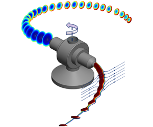


1 Introduction
Large surface-to-volume ratio, high porosity and special mechanical properties such as mechanical strength make nanofibres highly attractive in a broad spectrum of medical and industrial applications (Huang et al. Reference Huang, Zhang, Kotaki and Ramakrishna2003). Therefore, there has been much interest in producing nanofibres via a number of methods, such as electrospinning, melt blowing and bicomponent fibre spinning (Nayak et al. Reference Nayak, Padhye, Kyratzis, Truong and Arnold2011). However, common nanofibre production methods suffer from limitations such as low throughputs and restrictions on the nanofibre material choice. The centrifugal spinning (CS) process has recently been used to produce nanofibres with production rates that are hundreds of times larger than those of other methods (such as electrospinning). In addition, CS provides the possibility of working with both polymer solutions and melts (Nayak et al. Reference Nayak, Padhye, Kyratzis, Truong and Arnold2011), a feature that is absent in many nanofibre production methods. The CS procedure is a simple approach in which fibres emanate from rotating nozzles under centrifugal force, forming highly curved jets. These curved jets are stretched during the process until they arrive at the collector that are placed away from the rotation centre. However, due to jet instabilities, jet breakup and bead formation may occur during the CS process. While CS is still being improved, a complete understanding of the process has been limited due to the presence of many parameters that control the flow dynamics, e.g. inertial, viscous, centrifugal, surface tension and aerodynamic forces, as well as solvent evaporation effects, polymer rheological properties, etc.
To date, several researchers have experimentally attempted to characterize the CS process for producing nanofibres, while considering the effects of different parameters: polymer solution temperature (Sedaghat, Taheri-Nassaj & Naghizadeh Reference Sedaghat, Taheri-Nassaj and Naghizadeh2006; Wang et al. Reference Wang, Shi, Liu, Secret and Chen2011); polymer concentration (Lu et al. Reference Lu, Li, Zhang, Xu, Fu, Lee and Zhang2013; Ren et al. Reference Ren, Pandit, Elkin, Denman, Cooper and Kotha2013); rotational speed and orifice diameter (Weitz et al. Reference Weitz, Harnau, Rauschenbach, Burghard and Kern2008; Badrossamay et al. Reference Badrossamay, Mcllwee, Goss and Parker2010; Vazquez, Vasquez & Lozano Reference Vazquez, Vasquez and Lozano2012; Mary et al. Reference Mary, Senthilram, Suganya, Nagarajan, Venugopal, Ramakrishna and Giri Dev2013; Padron et al. Reference Padron, Fuentes, Caruntu and Lozano2013); solution thermal treatment (Andrade et al. Reference Andrade, Santo, Costa and Lobo2017). Experimental work has also documented the effects of polymer rheological behaviours on CS. For example, Zhmayev et al. (Reference Zhmayev, Divvela, Ruo, Huang and Joo2015) and Ren et al. (Reference Ren, Ozisik, Kotha and Underhill2015) have studied the effect of the polymer solution viscoelasticity on the fibre radius and trajectory and the latter publication has also considered the effects of viscoelasticity and surface tension on the jet breakup. Although experimental methods can be used to study CS parametrically, one needs to devote a large amount of time and effort to deliver a comprehensive understanding of the process. Additionally, by relying only on experiments, analysing the effects of certain parameters such as air drag and solvent evaporation can be extremely difficult (if not impossible). This is where mathematical modelling can be employed as a promising alternative and an additional research method.
There are several mathematical techniques that can be pursued to model CS, among which the asymptotic methods (or the string models) are common, thanks to their simplicity. The asymptotic methods are based on the zeroth-order slender body theories, providing a simple framework to capture the jet behaviours. (Throughout this work, the terms ‘fibre’ and ‘jet’ are used interchangeably.) Using the asymptotic methods to model a slender curved jet, sets of governing equations (consisting of mass and stress balances along with kinematic and dynamic conditions at the jet interface) are represented in a curvilinear coordinate system to track the jet. The asymptotic methods have been developed by several authors, including Wallwork et al. (Reference Wallwork, Decent, King and Schulkes2002), Decent, King & Wallwork (Reference Decent, King and Wallwork2002), Panda (Reference Panda2006), Părău et al. (Reference Părău, Decent, Simmons, Wong and King2007) and Marheineke & Wegener (Reference Marheineke and Wegener2009), to name but a few. Through these studies the effects of gravity, surface tension and polymer solution viscosity on the jet trajectory, radius and instability have been considered for different applications, e.g. prilling or glass particle production processes, which share similarities with CS in that they produce microfibres or nanofibres. Furthermore, shear thinning and viscoelastic effects have been investigated on the curved jet instability by Uddin, Decent & Simmons (Reference Uddin, Decent and Simmons2008), Uddin & Decent (Reference Uddin and Decent2009, Reference Uddin and Decent2010), Hawkins et al. (Reference Hawkins, Gurney, Decent, Simmons and Uddin2010), Alsharif & Uddin (Reference Alsharif and Uddin2015), Alsharif, Uddin & Afzaal (Reference Alsharif, Uddin and Afzaal2015) and Marheineke et al. (Reference Marheineke, Liljegren-Sailer, Lorenz and Wegener2016). Despite their simplicity and popularity, however, the asymptotic methods suffer from near-orifice singularities, strictly limiting their applications to parameters ranges corresponding to low-viscosity jets in slow rotations, as shown in detail by Götz et al. (Reference Götz, Klar, Unterreiter and Wegener2008) and Arne et al. (Reference Arne, Marheineke, Meister and Wegener2010). In fact, there are no physically relevant stationary solutions for curved jets if  $ReRb^{2}<1$ (where
 $Re$ is the Reynolds number and
 $Rb$ the Rossby number), which is likely the operating range of any CS process.
To avoid singularities in the string models and to predict the jet behaviours for a wide range of key parameters, one can rely on the rod model in which fully coupled conservation equations including mass, linear and angular momentum are solved (see e.g. Mahadevan & Keller Reference Mahadevan and Keller1996; Ribe Reference Ribe2004; Ribe, Habibi & Bonn Reference Ribe, Habibi and Bonn2006). For glass wool spinning applications, Arne et al. (Reference Arne, Marheineke, Meister and Wegener2010) developed a Cosserat rod theory to model a curved jet in a two-dimensional (2-D) stationary frame, which they later extended to a 3-D transient problem (Arne et al. Reference Arne, Marheineke, Meister, Schiessl and Wegener2015). In another attempt to remove the string model singularity, Arne, Marheineke & Wegener (Reference Arne, Marheineke and Wegener2011b) used an interface condition at which the solver switched from the rod to string model to eliminate the fibre angle boundary condition. Alternatively, to remove the near-nozzle singularity for CS applications, one can also use a regularization approach yielding a stable solution (Taghavi & Larson Reference Taghavi and Larson2014a,Reference Taghavi and Larsonb; Noroozi et al. Reference Noroozi, Alamdari, Arne, Larson and Taghavi2017).
When using the asymptotic methods to derive the curved jet equations, most of the previous studies assumed that the jet baseline torsion can be ignored, making it possible to use the orthogonal curvilinear coordinate system. Alternatively, Shikhmurzaev & Sisoev (Reference Shikhmurzaev and Sisoev2017) considered the effect of torsion when deriving the equations, leading to non-orthogonal basis vectors the terms of which they projected onto the orthonormal Frenet basis. Ignoring the jet cross-section deformation due to torsion, Panda (Reference Panda2006) and Marheineke & Wegener (Reference Marheineke and Wegener2009) used the Bishop frame (Bishop Reference Bishop1975) to provide coordinates of the curved jet and thereby avoid a cumbersome derivation of the governing equations in the non-orthogonal curvilinear coordinate system. On the other hand, Decent et al. (Reference Decent, Părău, Simmons and Uddin2018) mathematically showed that, when torsion is of  $O(1)$ or less, it has no effect on the jet behaviour when the jet is slender. In a recent study, Alsharif et al. (Reference Alsharif, Decent, Părău, Simmons and Uddin2018) analytically showed that, even at large rotation speeds, torsion is important only near the nozzle.
In this novel work, we rely on our experiments using a home-made CS set-up to fabricate polymer nanofibres at high rotation speeds. The input parameters in our experiments include, for example, the polymer properties (viscosity, surface tension coefficient, etc.) and the CS set-up operational and geometrical parameters (e.g. the rotation speed), while the output parameters are mainly the trajectory and radius of a curved viscous jet produced in the CS process, obtained via image processing techniques. Inspired by our experiments, we attempt to derive a rigorous, comprehensive string model to predict the behaviours of a viscous jet, in a non-orthogonal curvilinear coordinate system. Although our model is based on Newtonian fluid assumptions, it considers all the other key operational and geometrical parameters in a typical CS process. Our model analyses the main flow parameters including viscous, inertial, rotational, surface tension, gravitational, solvent evaporation and aerodynamic effects, using the key dimensionless groups that govern the flow.
The outline of the paper is as follows. In § 2 we present the material and methods used to perform our CS laboratory experiments and we explain our observations; furthermore, we introduce the phenomena and forces involved in our CS process. In § 3, inspired by our experimental observations, we formulate our mathematical model, including the governing equations, the assumptions and the asymptotic method to simplify the equations. In § 4, we first successfully compare our experimental and model results, and then we proceed to explore parametrically the effects of various flow parameters on the jet flow. Finally in § 5, we conclude the paper with a brief summary of the main findings.
2 Experiments
In this section, we briefly discuss our experimental set-up, and the materials and methods of our experiments. Then, we briefly review our general experimental observations, which we will later use to motivate the development of an appropriate asymptotic model. We also present the key parameters and their ranges in our experiments, which will later serve as the inputs for the asymptotic model.
2.1 Experimental description, set-up and methods
To systematically explain the CS process and the phenomena involved, let us divide a typical CS process into three stages. In the first stage, a polymeric solution is placed into a rotating chamber, known as a spinneret, whose rotation speed about its symmetry axis is  $\unicode[STIX]{x1D6FA}~\text{rad}~\text{s}^{-1}$. Under the so-called centrifugal force due to the spinneret rotation, the polymer solution is pushed towards the nozzle exit. During this stage, the polymer solution flow is affected by various effects, such as the spinneret and nozzle wall friction, as well as viscous and surface forces. In stage two, due to the large
 $\unicode[STIX]{x1D6FA}$, creating strong centrifugal forces that overcome the surface and viscous forces, the polymer solution emanates from the nozzle and it is extended as a curved fibre jet. As the fibre moves away from the nozzle, it significantly thins until it meets the collector that is placed away from the rotation centre (figure 1). During this stage, centrifugal, viscous, inertial, gravitational, as well as aerodynamic (air drag) and evaporation effects act on the fibre trajectory and the thinning process. Finally, in stage three, the fibre sits on the collector, while the evaporation continues. The fibre is then gathered from the collector. In the current work, we focus on analysing stage two of the CS process.
In practice, spinnerets with many nozzles are used to increase the CS device performance, producing nanofibres in large quantities. However, for simplicity in this study, a CS device based on a two-nozzle system with straight nozzles is employed, as schematically sketched in figure 1. As can be seen, stationary rods are placed at an adjustable distance acting as the collector arranged in a circle around the rotation centre.
(a) A schematic view of our CS process along with the accessories. The fibre, nozzle and collector are marked by arrows. The nozzle inner diameter is marked by  $a$, the spinneret radius by
 $s_{0}$ and the radial position of the collector with respect to the rotation centre by
 ${\mathcal{R}}_{collector}$. (b) A closer view of the fibre showing the forces and the phenomena involved. In the left and right images, there are several other parameters related to the model so they are referred to and explained in the model section.

The experiments are performed using polymer solutions made of Poly(ethylene oxide) (PEO, Aldrich). To obtain a homogeneous solution, a stock solution of each sample is prepared, first by dissolving PEO in deionized water at room temperature and then mixing it for 5 days. Then, several solutions are prepared by diluting the stock solution sample. Different sets of experiments are performed using PEO solutions with different molecular weights and at different concentrations, named sample (I), sample (II) and sample (III), as shown in table 1.
Polymer solution samples used in our work.  $M_{v}$ denotes the molecular weight. Data for sample (III) are extracted from Bahlouli et al. (Reference Bahlouli, Bekkour, Benchabane, Hemar and Nemdili2013).

Our experimental parameters (in dimensional form) and their relevant ranges are given in table 2. The geometrical parameters, i.e.  $a$,
 $s_{0}$ and
 ${\mathcal{R}}_{collector}$, are directly measured;
 $U_{noz}$ is calculated based on the mass flow rate of the jet flow from the nozzles,
 $\unicode[STIX]{x1D6FA}$ is monitored and measured via a data acquisition box (USB-6002),
 $RH^{\ast }$ is measured by a simple hygrometer,
 $\unicode[STIX]{x1D70C}_{noz}$ by a high-precision density meter (Anton Paar DMA 35),
 $\unicode[STIX]{x1D707}_{noz}$ by an advanced rheometer (DHR3 TA Instrument) and finally
 $\unicode[STIX]{x1D70E}_{noz}$ by a tensiometer (K100, KRUSS GmbH). Here, the subscript ‘
 $noz$’ marks an estimation of the experimental fluid property at the nozzle exit. Note that the experimental fluid has nearly a constant viscosity over a wide range of shear rates (at a fixed concentration), which allows one to ignore shear thinning and rely on the measured viscosity at small shear rates as a representative value for
 $\unicode[STIX]{x1D707}_{noz}$. To estimate the other parameters in table 2, e.g.
 $\unicode[STIX]{x1D70C}^{\ast }$,
 $D_{s}^{\ast }$,
 $p_{vap}$, etc., literature data or the existing empirical correlations are used, as detailed in appendix A.
Experimental parameters (dimensional) and their ranges in our work. The ranges are based on the ambient temperature ( $\unicode[STIX]{x1D703}=298~\text{K}$) and pressure (
 $\hat{p}=10^{5}$ Pa). The subscript
 $noz$ marks the polymer solution jet parameters at the nozzle exit. These parameters are assumed to be uniform within the cross-section at the nozzle exit. The asterisk (
 $\ast$) marks the parameters that are associated with the surrounding air. These parameters are also assumed to remain constant for each experiment.

To analyse the trajectory and the thinning of the fibre jet, top-view images of the process are taken using a high-speed camera (Photron FASTCAM Mini UX100, resolution up to 800 000 f.p.s.) along with powerful LED lamps (A-LED-W150 High Intensity). See figure 1 for the position of the camera and the lights. As significant fibre thinning is expected near the nozzle exit, our camera’s field of view is focused on this region.
To obtain the fibre trajectory and fibre radius at different positions, a quantitative image analysis based on the light intensity is implemented. To provide homogeneous illumination for better visualization of the curved fibres, the LED lamps are located at two different positions over the spinneret safety box equipped with diffusive sheets. To ensure the accuracy of extracted data, only high portions of images with high contrast are used. To capture the fibre boundary, a modified Canny edge detector is coded in Matlab. In this method, an image is first smoothed using a Gaussian filter to reduce noise. Afterwards, the intensity gradients in the image are located and the fibre edges are determined using a threshold set to a conventional value of 0.9. Spurious edges with no connection with the main continuous edges are subsequently removed. Finally, the trajectory and the radius of the fibre jet as it travels through the surrounding air are determined.
2.2 Key experimental observations and parameters to develop an appropriate model
As mentioned before, our experiments are focused on analysing the jet flow outside the nozzle, especially at longer times after the jet end has reached the collector. An example of the time-dependent jet trajectory is shown in figure 2(a), where an image sequence (top view) of the process can be seen. The trajectory of the jet is highly curved due to the rotational forces, as the jet moves away from the rotation centre, in a direction opposite to that of the spinneret rotation. The jet quickly thins under the action of various forces into a fibre, which is then collected on the collector (outside the field of view). In a frame rotating with the spinneret, figure 2(b) depicts the jet trajectories of figure 2(a) (at four different times). Interestingly, the trajectories at long times superimpose and the fibre in the rotating frame seems to follow the same path at different times. This implies that the behaviour of the fibre at long times is nearly steady state in the rotating frame. Our examinations of the fibre trajectory at long times for different samples and with different operating conditions reveal the same behaviours (omitted for brevity).
Trajectory of a single fibre at four different times: (a) experimental image sequence at the time interval of approximately 4 ms; (b) superposition of the corresponding fibre trajectories in a frame of reference moving with the spinneret. The field of view in all the images on the left and the figure on the right is  $149\times 42~\text{mm}^{2}$. The solution is sample (I), and the experimental parameters are
 $\unicode[STIX]{x1D6FA}=628~\text{rad}~\text{s}^{-1}$,
 ${\mathcal{R}}_{collector}=20~\text{cm}$,
 $a=0.58~\text{mm}$ and
 $RH^{\ast }=50\,\%$.

Based on these experimental observations, it is clear that the development of a steady-state thin-fibre model is appropriate to gain a deeper understanding of our experiments, by delivering predictions of the fibre trajectory, radius, etc., as well as the fibre features that are not accessible during a typical experiment (e.g. fibre viscosity or polymer concentration). The first step, however, is to introduce the phenomena and forces that are important in our experiments (as schematically depicted in the right image of figure 1). Various internal and external forces affect the fibre; the fibre internal forces balancing the external ones are inertial, surface tension and viscous forces. The latter two act to reduce the fibre velocity and its thinning while the former one acts to increase the fibre velocity and its thinning. In addition, centrifugal, Coriolis, aerodynamic and gravitational forces also affect the fibre trajectory and radius. Throughout the thinning domain, polymer solvent evaporation occurs, making the fibre radius smaller, while increasing the overall viscosity of the fibre without much affecting its density.
Definitions of dimensionless groups along with their ranges of values in our experiments. The dimensional parameters used to define the dimensionless ones are given in table 2. The dimensional and dimensionless parameters describing properties in the air are marked with an asterisk ( $\ast$).

Based on the forces and phenomena involved in our experiments, table 3 introduces several relevant dimensionless numbers. In this table,  $Rb$,
 $Re$,
 $We$ and
 $Fr$ are related to the polymer solution and denote the ratios, of inertial to, respectively, rotational, viscous, surface tension and gravitational forces. On the other hand,
 $Re^{\ast }$ describes the ratio of inertial to viscous terms in air. In addition,
 $Pe$ and
 $Pe^{\ast }$ express the advective to diffusive transport rate of the polymer in the solvent and the solvent in air, respectively. Similarly,
 $Sc$ and
 $Sc^{\ast }$ are Schmidt numbers, expressing the ratios of viscous to molecular diffusion rates, defined as
 $Pe/\unicode[STIX]{x1D700}Re$ and
 $Pe^{\ast }/Re^{\ast }$, respectively. Here,
 ${\mathcal{R}}$ denotes the dimensionless collector distance with respect to the rotation centre. Finally,
 $c_{sa}^{\ast }$ in our work mainly depends on the relative humidity in air, and quantifies the dimensionless concentration of water in air. Based on our experimental parameters (see table 2), the range of each dimensionless number is also presented in table 3.
For practitioners and experimentalists, the dimensionless groups introduced above can also be described as dimensionless physical quantities, highlighting the most natural variables. For example, given a constant flow rate, density and geometrical parameters in an experiment,  $Rb$,
 $Re$,
 $We$,
 $Pe$,
 $Re^{\ast }$ and
 $Pe^{\ast }$ may be interpreted as the inverse dimensionless numbers for rotation rate, polymer solution viscosity, surface tension, solvent diffusivity in polymer solution, air viscosity and solvent diffusivity in air, respectively.
In the next section, we will develop an appropriate mathematical thin-fibre model which relies on our experimental observations, and the dimensionless groups and their ranges discussed above.
3 Problem formulation
In this section, motivated by the experimental observations in the previous section, the governing equations describing the CS process for a viscous jet are laid out. Inspired by our experiments, a single curved jet is considered to emerge from a nozzle, thinning through the computational domain. The jet fluid is considered to be incompressible, and it is described as a mixture of two components, solvent and polymer, which are assumed as interpenetrable continua. Considering a rotating reference frame in Cartesian coordinates  $(x,y,z)$ in which the nozzle is fixed, one can write the motion, continuity and convection–diffusion equations at steady state as (Bird, Stewart & Lightfoot Reference Bird, Stewart and Lightfoot2007)
 $$\begin{eqnarray}\displaystyle & \displaystyle \underbrace{\boldsymbol{v}\boldsymbol{\cdot }\unicode[STIX]{x1D735}\boldsymbol{v}}_{\boldsymbol{f}_{inertial}}=\underbrace{-\unicode[STIX]{x1D735}p}_{\boldsymbol{f}_{pressure}}+\underbrace{\frac{1}{Re}\unicode[STIX]{x1D735}\boldsymbol{\cdot }\unicode[STIX]{x1D72B}}_{\boldsymbol{f}_{viscous}}+\underbrace{\frac{\boldsymbol{g}}{Fr^{2}}}_{\boldsymbol{f}_{gravity}}\underbrace{-\frac{2}{Rb}\;\unicode[STIX]{x1D734}\times \boldsymbol{v}}_{\boldsymbol{f}_{Coriolis}}\underbrace{-\frac{1}{Rb^{2}}\unicode[STIX]{x1D734}\times (\unicode[STIX]{x1D734}\times \boldsymbol{d})}_{\boldsymbol{f}_{centrifugal}}, & \displaystyle\end{eqnarray}$$
 $$\begin{eqnarray}\displaystyle & \displaystyle \unicode[STIX]{x1D735}\boldsymbol{\cdot }\boldsymbol{v}=0, & \displaystyle\end{eqnarray}$$
 $$\begin{eqnarray}\displaystyle & \displaystyle \boldsymbol{v}\boldsymbol{\cdot }\unicode[STIX]{x1D735}c=\frac{1}{Pe}\unicode[STIX]{x1D6FB}^{2}c, & \displaystyle\end{eqnarray}$$
in which  $\boldsymbol{v}=(v^{1},v^{2},v^{3})$ is the velocity field,
 $p$ the pressure field,
 $\boldsymbol{g}=(0,-1,0)$ the gravity acceleration vector,
 $\unicode[STIX]{x1D734}=(0,1,0)$ the angular velocity vector,
 $\boldsymbol{d}$ the position vector and
 $\unicode[STIX]{x1D72B}$ the deviatoric stress tensor. For clarity, the forces associated with the different terms in (3.1), are labelled by
 $\boldsymbol{f}$ with appropriate subscripts. In addition,
 $c$ denotes the polymer scaler concentration. Hereafter, all the variable/parameters are presented in dimensionless form, using
 $s_{0}$ as length scale (except for the fibre radius which is scaled with
 $a$),
 $U_{noz}$ as velocity scale and
 $\unicode[STIX]{x1D70C}_{noz}U_{noz}^{2}$ as stress/pressure scale. While the jet density and the surface tension coefficient are assumed to be constants, the jet viscosity is assumed to vary along the jet, so its value is normalized by the nozzle value, i.e.
 $\unicode[STIX]{x1D707}_{noz}$. The definitions of the dimensionless parameters are given in table 3.
Using the full set of (i.e. equations (3.1)–(3.3) along with the boundary conditions presented later), describing the jet dynamics via a direct numerical simulation of a long 3-D nanosized jet is extremely costly (if not impossible). Therefore, to make the numerical procedure feasible, it is typical to use a one-dimensional uniaxial two-phase flow model, arising from cross-sectional averaging of the key quantities. However, since the radial diffusion controls the solvent mass transfer in our case, equation (3.3) requires a two-dimensional solution involving axial and radial variables. Thus, in this work we will first derive equations (3.1) and (3.2) in the axial direction, based on the cross-averaged values of various quantities, and then develop the concentration–diffusion equation (3.3) in the radial–axial plane.
3.1 Coordinate system and basis vectors
To render our set of equations one-dimensional and to ease the solution method, we rely on the curvilinear coordinate system  $(s,r,\unicode[STIX]{x1D711})$ to track the jet behaviours. Here,
 $s$ is the arc length through the jet baseline and
 $(r,\unicode[STIX]{x1D711})$ are the plane polar coordinates in the radial and azimuthal directions, respectively, describing the jet cross-section. As our curvilinear coordinate system is non-orthogonal due to non-zero baseline torsion assumptions, we need some basic relations to derive the differential terms in our set of equations, using the differential geometry approach. The basis vectors in our coordinate system are defined as
 $\boldsymbol{g}_{1}$,
 $\boldsymbol{g}_{2}$ and
 $\boldsymbol{g}_{3}$ corresponding to the
 $s$,
 $r$ and
 $\unicode[STIX]{x1D711}$ directions, respectively. To present the baseline of the jet, we choose the Cartesian coordinate system as a fixed reference frame. We derive our set of equations in each direction and then represent the projection of each one onto the Frenet basis (i.e. orthonormal) as final equations. The coordinate systems and the corresponding basis vectors are sketched in figure 1.
The jet baseline position vector,  $\boldsymbol{D}(s)$ in the Cartesian coordinate system can be expressed as follows:
 $$\begin{eqnarray}\boldsymbol{D}(s)=X(s)\hat{\boldsymbol{x}}+Y(s)\hat{\boldsymbol{y}}+Z(s)\hat{\boldsymbol{z}},\end{eqnarray}$$
in which  $\hat{\boldsymbol{x}}$,
 $\hat{\boldsymbol{y}}$,
 $\hat{\boldsymbol{z}}$ are the Cartesian basis vectors. Based on equation (3.4), the Frenet basis vectors, i.e. tangential
 $\boldsymbol{T}(s)$, principal normal
 $\boldsymbol{N}(s)$ and binormal
 $\boldsymbol{B}(s)$ can be defined as
 $$\begin{eqnarray}\displaystyle & \displaystyle \boldsymbol{T}=\frac{\text{d}\boldsymbol{D}}{\text{d}s}=X_{,s}\,\hat{\boldsymbol{x}}+Y_{,s}\,\hat{\boldsymbol{y}}+Z_{,s}\,\hat{\boldsymbol{z}}, & \displaystyle\end{eqnarray}$$
 $$\begin{eqnarray}\displaystyle & \displaystyle \boldsymbol{N}=\frac{\text{d}\boldsymbol{T}}{\text{d}s}\left|\frac{\text{d}\boldsymbol{T}}{\text{d}s}\right|^{-1}=\frac{X_{,ss}\,\hat{\boldsymbol{x}}+Y_{,ss}\,\hat{\boldsymbol{y}}+Z_{,ss}\,\hat{\boldsymbol{z}}}{\sqrt{(X_{,ss})^{2}+(Y_{,ss})^{2}+(Z_{,ss})^{2}}}, & \displaystyle\end{eqnarray}$$
 $$\begin{eqnarray}\displaystyle & \displaystyle \boldsymbol{B}=\boldsymbol{T}\times \boldsymbol{N}=\frac{(Y_{,s}Z_{,ss}-Y_{,ss}Z_{,s})\hat{\boldsymbol{x}}+(Z_{,s}X_{,ss}-Z_{,ss}X_{,s})\hat{\boldsymbol{y}}+(X_{,s}Y_{,ss}-X_{,ss}Y_{,s})\hat{\boldsymbol{z}}}{\sqrt{(X_{,ss})^{2}+(Y_{,ss})^{2}+(Z_{,ss})^{2}}}. & \displaystyle\end{eqnarray}$$
The derivatives of the Frenet basis with respect to the arc length,  $s$, can be computed as
 $$\begin{eqnarray}\frac{\text{d}\boldsymbol{T}}{\text{d}s}=\unicode[STIX]{x1D705}\boldsymbol{N},\quad \frac{\text{d}\boldsymbol{N}}{\text{d}s}=-\unicode[STIX]{x1D705}\boldsymbol{T}+\unicode[STIX]{x1D70F}\boldsymbol{B},\quad \frac{\text{d}\boldsymbol{B}}{\text{d}s}=-\unicode[STIX]{x1D70F}\boldsymbol{N},\end{eqnarray}$$
in which  $\unicode[STIX]{x1D705}$ and
 $\unicode[STIX]{x1D70F}$ stand for the baseline curvature and torsion expressed as
 $$\begin{eqnarray}\displaystyle & \displaystyle \unicode[STIX]{x1D705}(s)=\sqrt{(X_{,ss})^{2}+(Y_{,ss})^{2}+(Z_{,ss})^{2}}, & \displaystyle\end{eqnarray}$$
 $$\begin{eqnarray}\displaystyle & \displaystyle \unicode[STIX]{x1D70F}(s)=\frac{X_{,sss}(Y_{,s}Z_{,ss}-Y_{,ss}Z_{,s})+Y_{,sss}(X_{,ss}Z_{,s}-Z_{,ss}X_{,s})+Z_{,sss}(X_{,s}Y_{,ss}-X_{,ss}Y_{,s})}{(Y_{,s}Z_{,ss}-Y_{,ss}Z_{,s})^{2}+(X_{,ss}Z_{,s}-Z_{,ss}X_{,s})^{2}+(X_{,s}Y_{,ss}-X_{,ss}Y_{,s})^{2}}. & \displaystyle \nonumber\\ \displaystyle & & \displaystyle\end{eqnarray}$$
Whenever appropriate we use  $k_{,s}$ as the ordinary derivative of an arbitrary function
 $k$ and
 $\left.k\right|_{s}$ as the covariant derivative of
 $k$ with respect to
 $s$. We note that if
 $k$ is a differentiable scalar function, its ordinary partial derivative is equal to its covariant derivative. We also define
 $\left\langle k\right\rangle _{T}$ as the projection of a given vector
 $\boldsymbol{k}$ onto an arbitrary base vector such as
 $\boldsymbol{T}$.
To find the flow field of the jet, we need to define the radius vector of an arbitrary point in the Cartesian and curvilinear coordinate systems as (see figure 1)
 $$\begin{eqnarray}\displaystyle & \displaystyle \boldsymbol{d}(x,y,z)=x\,\hat{\boldsymbol{x}}+y\,\hat{\boldsymbol{y}}+z\,\hat{\boldsymbol{z}}, & \displaystyle\end{eqnarray}$$
 $$\begin{eqnarray}\displaystyle & \displaystyle \boldsymbol{d}(s,r,\unicode[STIX]{x1D711})=\boldsymbol{D}(s)+\unicode[STIX]{x1D700}r\cos (\unicode[STIX]{x1D711})\boldsymbol{N}+\unicode[STIX]{x1D700}r\sin (\unicode[STIX]{x1D711})\boldsymbol{B}, & \displaystyle\end{eqnarray}$$
where  $\unicode[STIX]{x1D700}=a/s_{0}$ is the aspect ratio. Using equation (3.12), we can find the basis vectors in the curvilinear coordinate system as
 $$\begin{eqnarray}\boldsymbol{g}_{i}=\frac{\unicode[STIX]{x2202}\boldsymbol{d}}{\unicode[STIX]{x2202}s^{i}}\quad (i=1,2,3)\text{ and }(s^{1}=s,s^{2}=r,s^{3}=\unicode[STIX]{x1D711}),\end{eqnarray}$$
and therefore,
 $$\begin{eqnarray}\displaystyle & \displaystyle \boldsymbol{g}_{1}=\frac{\unicode[STIX]{x2202}\boldsymbol{d}}{\unicode[STIX]{x2202}s}=(1-\unicode[STIX]{x1D700}r\cos (\unicode[STIX]{x1D711})\unicode[STIX]{x1D705})\boldsymbol{T}-(\unicode[STIX]{x1D700}r\sin (\unicode[STIX]{x1D711})\unicode[STIX]{x1D70F})\boldsymbol{N}+(\unicode[STIX]{x1D700}r\cos (\unicode[STIX]{x1D711})\unicode[STIX]{x1D70F})\boldsymbol{B}, & \displaystyle\end{eqnarray}$$
 $$\begin{eqnarray}\displaystyle & \displaystyle \boldsymbol{g}_{2}=\frac{\unicode[STIX]{x2202}\boldsymbol{d}}{\unicode[STIX]{x2202}r}=(\unicode[STIX]{x1D700}\cos (\unicode[STIX]{x1D711}))\boldsymbol{N}+(\unicode[STIX]{x1D700}\sin (\unicode[STIX]{x1D711}))\boldsymbol{B}, & \displaystyle\end{eqnarray}$$
 $$\begin{eqnarray}\displaystyle & \displaystyle \boldsymbol{g}_{3}=\frac{\unicode[STIX]{x2202}\boldsymbol{d}}{\unicode[STIX]{x2202}\unicode[STIX]{x1D711}}=(-\unicode[STIX]{x1D700}r\sin (\unicode[STIX]{x1D711}))\boldsymbol{N}+(\unicode[STIX]{x1D700}r\cos (\unicode[STIX]{x1D711}))\boldsymbol{B}. & \displaystyle\end{eqnarray}$$
To define whether we are dealing with an irregular basis, i.e. one that is non-orthogonal, non-normalized and/or non-right handed, we need to define the metric tensor using  $g_{ij}=\boldsymbol{g}_{i}\boldsymbol{\cdot }\boldsymbol{g}_{j}$, which can be represented in matrix form as
 $$\begin{eqnarray}\left.\begin{array}{@{}c@{}}\displaystyle (g_{ij})=\left(\begin{array}{@{}ccc@{}}(1-\unicode[STIX]{x1D700}r\unicode[STIX]{x1D705}\cos (\unicode[STIX]{x1D711}))^{2}+(\unicode[STIX]{x1D700}r\unicode[STIX]{x1D70F})^{2} & 0 & (\unicode[STIX]{x1D700}r)^{2}\unicode[STIX]{x1D70F}\\ 0 & \unicode[STIX]{x1D700}^{2} & 0\\ (\unicode[STIX]{x1D700}r)^{2}\unicode[STIX]{x1D70F} & 0 & (\unicode[STIX]{x1D700}r)^{2}\\ \end{array}\right),\\ \displaystyle |g_{ij}|=\unicode[STIX]{x1D700}^{2}(1-\unicode[STIX]{x1D700}r\unicode[STIX]{x1D705}\cos (\unicode[STIX]{x1D711}))^{2}(\unicode[STIX]{x1D700}r)^{2},\end{array}\right\}\end{eqnarray}$$
in which  $|g_{ij}|$ stands for the determinant of the metric tensor. As can be seen, our local bases are neither orthogonal (due to existence of off-diagonal elements) nor normalized (due to non-unity of diagonal elements) as pointed out by Shikhmurzaev & Sisoev (Reference Shikhmurzaev and Sisoev2017). It is noted that some of the relations presented in this and the next subsections have been derived with alternative methods by Shikhmurzaev & Sisoev (Reference Shikhmurzaev and Sisoev2017), which we re-derive for the sake of completeness and verification. Using (3.17), we can simply compute the conjugate metric tensor
 $g^{ij}$ so that
 $g^{ik}\cdot g_{kj}=\unicode[STIX]{x1D6FF}_{j}^{i}$, in which
 $\unicode[STIX]{x1D6FF}_{j}^{i}$ is the Kronecker delta; therefore, we find
 $$\begin{eqnarray}(g^{ij})=\frac{\unicode[STIX]{x1D700}^{2}}{|g_{ij}|}\left(\begin{array}{@{}ccc@{}}(\unicode[STIX]{x1D700}r)^{2} & 0 & -(\unicode[STIX]{x1D700}r)^{2}\unicode[STIX]{x1D70F}\\ 0 & r^{2}(1-\unicode[STIX]{x1D700}r\unicode[STIX]{x1D705}\cos (\unicode[STIX]{x1D711}))^{2} & 0\\ -(\unicode[STIX]{x1D700}r)^{2}\unicode[STIX]{x1D70F} & 0 & (1-\unicode[STIX]{x1D700}r\unicode[STIX]{x1D705}\cos (\unicode[STIX]{x1D711}))^{2}+(\unicode[STIX]{x1D700}r\unicode[STIX]{x1D70F})^{2}\end{array}\right).\end{eqnarray}$$
Using (3.18) and (3.17) we can define the gradient operator  $\unicode[STIX]{x1D735}$ in our curvilinear coordinate system as
 $$\begin{eqnarray}\unicode[STIX]{x1D735}=g^{ik}\boldsymbol{g}_{k}\frac{\unicode[STIX]{x2202}}{\unicode[STIX]{x2202}s^{i}}=\left(\frac{1}{h^{2}}\boldsymbol{g}_{1}-\frac{\unicode[STIX]{x1D70F}}{h^{2}}\boldsymbol{g}_{3}\right)\frac{\unicode[STIX]{x2202}}{\unicode[STIX]{x2202}s}+\left(\frac{1}{\unicode[STIX]{x1D700}^{2}}\boldsymbol{g}_{2}\right)\frac{\unicode[STIX]{x2202}}{\unicode[STIX]{x2202}r}+\left(\frac{\unicode[STIX]{x1D709}^{2}}{\unicode[STIX]{x1D700}^{2}r^{2}h^{2}}\boldsymbol{g}_{3}-\frac{\unicode[STIX]{x1D70F}}{h^{2}}\boldsymbol{g}_{1}\right)\frac{\unicode[STIX]{x2202}}{\unicode[STIX]{x2202}\unicode[STIX]{x1D711}},\end{eqnarray}$$
in which  $h=1-\unicode[STIX]{x1D700}r\unicode[STIX]{x1D705}\cos (\unicode[STIX]{x1D711})$ and
 $\unicode[STIX]{x1D709}=(h^{2}+(\unicode[STIX]{x1D700}r\unicode[STIX]{x1D70F})^{2})^{1/2}$.
To find the variations of the basis vectors in space, we need to find the connection coefficients or the Christoffel symbols of the second kind ( $\unicode[STIX]{x1D6E4}_{ij}^{k}$). With this goal, we use the general relation that can be found in standard textbooks (e.g. Brannon Reference Brannon2004) as
 $$\begin{eqnarray}\unicode[STIX]{x1D6E4}_{ij}^{k}=\frac{g^{kl}}{2}\left(\frac{\unicode[STIX]{x2202}g_{jl}}{\unicode[STIX]{x2202}s^{i}}+\frac{\unicode[STIX]{x2202}g_{il}}{\unicode[STIX]{x2202}s^{j}}-\frac{\unicode[STIX]{x2202}g_{ij}}{\unicode[STIX]{x2202}s^{l}}\right),\end{eqnarray}$$
in which  $i,j,k$ and
 $l$ are dummy indices. Using equations (3.17), (3.18) and (3.20), we have
 $$\begin{eqnarray}\left.\begin{array}{@{}c@{}}\displaystyle \unicode[STIX]{x1D6E4}_{11}^{1}=\frac{\unicode[STIX]{x1D700}r}{h}(-\text{cos}(\unicode[STIX]{x1D711})\unicode[STIX]{x1D705}_{,s}+\unicode[STIX]{x1D705}\unicode[STIX]{x1D70F}\sin (\unicode[STIX]{x1D711})),\\ \displaystyle \unicode[STIX]{x1D6E4}_{11}^{2}=\frac{1}{\unicode[STIX]{x1D700}}(h\cos (\unicode[STIX]{x1D711})\unicode[STIX]{x1D705}-\unicode[STIX]{x1D700}r\unicode[STIX]{x1D70F}^{2}),\\ \displaystyle \unicode[STIX]{x1D6E4}_{11}^{3}=\frac{\unicode[STIX]{x1D700}r\unicode[STIX]{x1D70F}}{h}(\cos (\unicode[STIX]{x1D711})\unicode[STIX]{x1D705}_{,s}-\unicode[STIX]{x1D705}\unicode[STIX]{x1D70F}\sin (\unicode[STIX]{x1D711}))-\frac{h}{\unicode[STIX]{x1D700}r}\unicode[STIX]{x1D705}\sin (\unicode[STIX]{x1D711})+\unicode[STIX]{x1D70F}_{,s},\\ \displaystyle \unicode[STIX]{x1D6E4}_{12}^{1}=\unicode[STIX]{x1D6E4}_{21}^{1}=-\frac{\unicode[STIX]{x1D700}\unicode[STIX]{x1D705}}{h}\cos (\unicode[STIX]{x1D711}),\quad \unicode[STIX]{x1D6E4}_{12}^{2}=\unicode[STIX]{x1D6E4}_{21}^{2}=0,\\ \displaystyle \unicode[STIX]{x1D6E4}_{12}^{3}=\unicode[STIX]{x1D6E4}_{21}^{3}=\unicode[STIX]{x1D70F}\left(\frac{\unicode[STIX]{x1D700}\unicode[STIX]{x1D705}}{h}\cos (\unicode[STIX]{x1D711})+\frac{1}{r}\right),\\ \displaystyle \unicode[STIX]{x1D6E4}_{13}^{1}=\unicode[STIX]{x1D6E4}_{31}^{1}=\frac{\unicode[STIX]{x1D700}r\unicode[STIX]{x1D705}}{h}\sin (\unicode[STIX]{x1D711}),\quad \unicode[STIX]{x1D6E4}_{13}^{2}=\unicode[STIX]{x1D6E4}_{31}^{2}=-r\unicode[STIX]{x1D70F},\\ \displaystyle \unicode[STIX]{x1D6E4}_{13}^{3}=\unicode[STIX]{x1D6E4}_{31}^{3}=-\frac{\unicode[STIX]{x1D700}r\unicode[STIX]{x1D705}\unicode[STIX]{x1D70F}}{h}\sin (\unicode[STIX]{x1D711}),\\ \unicode[STIX]{x1D6E4}_{22}^{1}=\unicode[STIX]{x1D6E4}_{22}^{2}=\unicode[STIX]{x1D6E4}_{22}^{3}=0,\quad \unicode[STIX]{x1D6E4}_{33}^{1}=\unicode[STIX]{x1D6E4}_{33}^{3}=0,\quad \unicode[STIX]{x1D6E4}_{33}^{2}=-r,\quad \unicode[STIX]{x1D6E4}_{23}^{1}=\unicode[STIX]{x1D6E4}_{32}^{1}=0,\\ \unicode[STIX]{x1D6E4}_{23}^{2}=\unicode[STIX]{x1D6E4}_{32}^{2}=0,\quad \unicode[STIX]{x1D6E4}_{23}^{3}=\unicode[STIX]{x1D6E4}_{32}^{3}=\frac{1}{r}.\end{array}\right\}\end{eqnarray}$$
From (3.21) we can now find the gradients of the basis vectors in our curvilinear coordinate system using
 $$\begin{eqnarray}\frac{\unicode[STIX]{x2202}\boldsymbol{g}_{i}}{\unicode[STIX]{x2202}s^{j}}=\unicode[STIX]{x1D6E4}_{ij}^{k}\boldsymbol{g}_{k}.\end{eqnarray}$$
In the next step, we will derive the governing equations that describe the curved jet dynamics in the uniaxial frame.
3.2 Governing equations
To compute the physical components of the velocity vectors (Malvern Reference Malvern1969), we need to normalize each basis vector by dividing it by its magnitude as
 $$\begin{eqnarray}\boldsymbol{v}=v^{i}\boldsymbol{g}_{\boldsymbol{ i}}=v^{i}|\boldsymbol{g}_{\boldsymbol{ i}}|\frac{\boldsymbol{g}_{\boldsymbol{i}}}{|\boldsymbol{g}_{\boldsymbol{i}}|}=v^{i}|\boldsymbol{g}_{\boldsymbol{ i}}|\hat{\boldsymbol{g}}_{\boldsymbol{i}},\end{eqnarray}$$
in which  $\hat{\boldsymbol{g}}_{\boldsymbol{i}}$ are the normalized basis vectors. Therefore, the physical components of the velocity vector (
 $u,v,w$) are
 $$\begin{eqnarray}u=v^{1}|\boldsymbol{g}_{\boldsymbol{ 1}}|=\unicode[STIX]{x1D709}v^{1},\quad v=v^{2}|\boldsymbol{g}_{\boldsymbol{ 2}}|=\unicode[STIX]{x1D700}v^{2},\quad w=v^{3}|\boldsymbol{g}_{\boldsymbol{ 3}}|=\unicode[STIX]{x1D700}rv^{3}.\end{eqnarray}$$
In the next step, we will derive the uniaxial equations to describe the jet dynamics and then the axial–radial convection–diffusion equation to consider the solvent evaporation. Afterwards, we will present the boundary conditions, followed by the solution algorithm needed to solve our sets of equations.
3.2.1 Continuity equation
Equation (3.2) in our curvilinear coordinate system for an incompressible fluid flow can be written as
 $$\begin{eqnarray}\frac{\unicode[STIX]{x2202}}{\unicode[STIX]{x2202}s^{i}}(Jv^{i})=0,\end{eqnarray}$$
in which  $J=|g_{ij}|^{1/2}$ is the mapping Jacobian. It is noted that to obtain equation (3.24) from (3.2), one should use
 $\unicode[STIX]{x1D6E4}_{ij}^{j}=\unicode[STIX]{x1D6E4}_{ji}^{j}=J^{-1}\unicode[STIX]{x2202}_{i}J$, the proof of which can be obtained from (3.20) or it can be found in any standard textbooks such as Synge & Schild (Reference Synge and Schild1978) and Sochi (Reference Sochi2016). After some algebra, we arrive at
 $$\begin{eqnarray}\displaystyle & & \displaystyle \frac{\unicode[STIX]{x2202}}{\unicode[STIX]{x2202}s}\left(\frac{u}{\unicode[STIX]{x1D709}}\right)+\frac{1}{\unicode[STIX]{x1D700}}\left(\frac{\unicode[STIX]{x2202}v}{\unicode[STIX]{x2202}r}+\frac{1}{r}\frac{\unicode[STIX]{x2202}w}{\unicode[STIX]{x2202}\unicode[STIX]{x1D711}}\right)-\frac{\unicode[STIX]{x1D700}r\cos (\unicode[STIX]{x1D711})\unicode[STIX]{x1D705}_{,s}}{h}\left(\frac{u}{\unicode[STIX]{x1D709}}\right)\nonumber\\ \displaystyle & & \displaystyle \quad +\,\left(\frac{1-2\unicode[STIX]{x1D700}r\unicode[STIX]{x1D705}\cos (\unicode[STIX]{x1D711})}{\unicode[STIX]{x1D700}rh}\right)v+\left(\frac{\unicode[STIX]{x1D705}\sin (\unicode[STIX]{x1D711})}{h}\right)w=0.\end{eqnarray}$$
3.2.2 Equations of motion
Here, we systematically derive each term in the equations of motion (3.1), i.e.  $\boldsymbol{f}_{inertial}$,
 $\boldsymbol{f}_{pressure}$,
 $\boldsymbol{f}_{viscous}$,
 $\boldsymbol{f}_{gravity}$,
 $\boldsymbol{f}_{Coriolis}$ and
 $\boldsymbol{f}_{centrifugal}$. To calculate the left-hand side of (3.1), we can make use of the definition of acceleration in a general coordinate system as
 $$\begin{eqnarray}\boldsymbol{v}\boldsymbol{\cdot }\unicode[STIX]{x1D735}\boldsymbol{v}=\left(v^{j}\left(\frac{\unicode[STIX]{x2202}v^{i}}{\unicode[STIX]{x2202}s^{j}}+v^{k}\unicode[STIX]{x1D6E4}_{jk}^{i}\right)\right)\boldsymbol{g}_{\boldsymbol{ i}}.\end{eqnarray}$$
Using equations (3.14)–(3.16) in combination with equation (3.26) and then projecting the resultant terms onto the Frenet basis, we have
 $$\begin{eqnarray}\displaystyle \boldsymbol{f}_{inertial}=\boldsymbol{v}\boldsymbol{\cdot }\unicode[STIX]{x1D735}\boldsymbol{v} & = & \displaystyle h\left[\frac{u}{\unicode[STIX]{x1D709}}\frac{\unicode[STIX]{x2202}}{\unicode[STIX]{x2202}s}\left(\frac{u}{\unicode[STIX]{x1D709}}\right)+\frac{1}{\unicode[STIX]{x1D700}}\left(v\frac{\unicode[STIX]{x2202}}{\unicode[STIX]{x2202}r}\left(\frac{u}{\unicode[STIX]{x1D709}}\right)+\frac{w}{r}\frac{\unicode[STIX]{x2202}}{\unicode[STIX]{x2202}\unicode[STIX]{x1D711}}\left(\frac{u}{\unicode[STIX]{x1D709}}\right)\right)\right.\nonumber\\ \displaystyle & & \displaystyle +\left.\left(\unicode[STIX]{x1D705}\unicode[STIX]{x1D70F}\sin (\unicode[STIX]{x1D711})-\cos (\unicode[STIX]{x1D711})\unicode[STIX]{x1D705}_{,s}\right)\frac{\unicode[STIX]{x1D700}ru^{2}}{h\unicode[STIX]{x1D709}^{2}}-2\left(v\cos (\unicode[STIX]{x1D711})-w\sin (\unicode[STIX]{x1D711})\right)\frac{\unicode[STIX]{x1D705}u}{h\unicode[STIX]{x1D709}}\right]\boldsymbol{T}\nonumber\\ \displaystyle & & \displaystyle +\,\left[\cos (\unicode[STIX]{x1D711})\left(\frac{u}{\unicode[STIX]{x1D709}}\frac{\unicode[STIX]{x2202}v}{\unicode[STIX]{x2202}s}+\frac{1}{\unicode[STIX]{x1D700}}\left(v\frac{\unicode[STIX]{x2202}v}{\unicode[STIX]{x2202}r}+\frac{w}{r}\frac{\unicode[STIX]{x2202}v}{\unicode[STIX]{x2202}\unicode[STIX]{x1D711}}\right)\right)\right.\nonumber\\ \displaystyle & & \displaystyle -\,\sin (\unicode[STIX]{x1D711})\left(\frac{u}{\unicode[STIX]{x1D709}}\frac{\unicode[STIX]{x2202}w}{\unicode[STIX]{x2202}s}+\frac{v}{\unicode[STIX]{x1D700}}\frac{\unicode[STIX]{x2202}w}{\unicode[STIX]{x2202}r}+\frac{w}{\unicode[STIX]{x1D700}r}\frac{\unicode[STIX]{x2202}w}{\unicode[STIX]{x2202}\unicode[STIX]{x1D711}}\right)\nonumber\\ \displaystyle & & \displaystyle -\,\unicode[STIX]{x1D700}r\unicode[STIX]{x1D70F}\sin (\unicode[STIX]{x1D711})\left(\frac{u}{\unicode[STIX]{x1D709}}\frac{\unicode[STIX]{x2202}}{\unicode[STIX]{x2202}s}\left(\frac{u}{\unicode[STIX]{x1D709}}\right)+\frac{v}{\unicode[STIX]{x1D700}}\frac{\unicode[STIX]{x2202}}{\unicode[STIX]{x2202}r}\left(\frac{u}{\unicode[STIX]{x1D709}}\right)+\frac{w}{\unicode[STIX]{x1D700}r}\frac{\unicode[STIX]{x2202}}{\unicode[STIX]{x2202}\unicode[STIX]{x1D711}}\left(\frac{u}{\unicode[STIX]{x1D709}}\right)\right)\nonumber\\ \displaystyle & & \displaystyle +\,\left(h\unicode[STIX]{x1D705}-\unicode[STIX]{x1D700}r\unicode[STIX]{x1D70F}^{2}\cos (\unicode[STIX]{x1D711})-\unicode[STIX]{x1D700}r\sin (\unicode[STIX]{x1D711})\unicode[STIX]{x1D70F}_{,s}\right)\frac{u^{2}}{\unicode[STIX]{x1D709}^{2}}\nonumber\\ \displaystyle & & \displaystyle -\,2\unicode[STIX]{x1D70F}\left(v\sin (\unicode[STIX]{x1D711})+w\cos (\unicode[STIX]{x1D711})\right)\frac{u}{\unicode[STIX]{x1D709}}\nonumber\\ \displaystyle & & \displaystyle -\left.\left(w\cos (\unicode[STIX]{x1D711})+v\sin (\unicode[STIX]{x1D711})\right)\frac{w}{\unicode[STIX]{x1D700}r}\right]\boldsymbol{N}\nonumber\\ \displaystyle & & \displaystyle +\,\left[\sin (\unicode[STIX]{x1D711})\left(\frac{u}{\unicode[STIX]{x1D709}}\frac{\unicode[STIX]{x2202}v}{\unicode[STIX]{x2202}s}+\frac{1}{\unicode[STIX]{x1D700}}\left(v\frac{\unicode[STIX]{x2202}v}{\unicode[STIX]{x2202}r}+\frac{w}{r}\frac{\unicode[STIX]{x2202}v}{\unicode[STIX]{x2202}\unicode[STIX]{x1D711}}\right)\right)\right.\nonumber\\ \displaystyle & & \displaystyle +\,\cos (\unicode[STIX]{x1D711})\left(\frac{u}{\unicode[STIX]{x1D709}}\frac{\unicode[STIX]{x2202}w}{\unicode[STIX]{x2202}s}+\frac{v}{\unicode[STIX]{x1D700}}\frac{\unicode[STIX]{x2202}w}{\unicode[STIX]{x2202}r}+\frac{w}{\unicode[STIX]{x1D700}r}\frac{\unicode[STIX]{x2202}w}{\unicode[STIX]{x2202}\unicode[STIX]{x1D711}}\right)\nonumber\\ \displaystyle & & \displaystyle +\,\unicode[STIX]{x1D700}r\unicode[STIX]{x1D70F}\cos (\unicode[STIX]{x1D711})\left(\frac{u}{\unicode[STIX]{x1D709}}\frac{\unicode[STIX]{x2202}}{\unicode[STIX]{x2202}s}\left(\frac{u}{\unicode[STIX]{x1D709}}\right)+\frac{v}{\unicode[STIX]{x1D700}}\frac{\unicode[STIX]{x2202}}{\unicode[STIX]{x2202}r}\left(\frac{u}{\unicode[STIX]{x1D709}}\right)+\frac{w}{\unicode[STIX]{x1D700}r}\frac{\unicode[STIX]{x2202}}{\unicode[STIX]{x2202}\unicode[STIX]{x1D711}}\left(\frac{u}{\unicode[STIX]{x1D709}}\right)\right)\nonumber\\ \displaystyle & & \displaystyle -\,\left(\unicode[STIX]{x1D700}r\unicode[STIX]{x1D70F}^{2}\sin (\unicode[STIX]{x1D711})+\unicode[STIX]{x1D700}r\cos (\unicode[STIX]{x1D711})\unicode[STIX]{x1D70F}_{,s}\right)\frac{u^{2}}{\unicode[STIX]{x1D709}^{2}}+2\unicode[STIX]{x1D70F}\left(v\cos (\unicode[STIX]{x1D711})-w\sin (\unicode[STIX]{x1D711})\right)\frac{u}{\unicode[STIX]{x1D709}}\nonumber\\ \displaystyle & & \displaystyle -\left.\left(w\sin (\unicode[STIX]{x1D711})-v\cos (\unicode[STIX]{x1D711})\right)\frac{w}{\unicode[STIX]{x1D700}r}\right]\boldsymbol{B}.\end{eqnarray}$$
Next, we derive the pressure gradient terms as
 $$\begin{eqnarray}\unicode[STIX]{x1D735}p=g^{ij}\frac{\unicode[STIX]{x2202}p}{\unicode[STIX]{x2202}s^{j}}\boldsymbol{g}_{\boldsymbol{i}},\end{eqnarray}$$
and, after projecting onto the Frenet basis, we find
 $$\begin{eqnarray}\displaystyle \boldsymbol{f}_{pressure}=-\unicode[STIX]{x1D735}p & = & \displaystyle -\left[\left(\frac{1}{h}\frac{\unicode[STIX]{x2202}p}{\unicode[STIX]{x2202}s}-\frac{\unicode[STIX]{x1D70F}}{h}\frac{\unicode[STIX]{x2202}p}{\unicode[STIX]{x2202}\unicode[STIX]{x1D711}}\right)\boldsymbol{T}\right.\nonumber\\ \displaystyle & & \displaystyle +\,\frac{1}{\unicode[STIX]{x1D700}}\left(\cos (\unicode[STIX]{x1D711})\frac{\unicode[STIX]{x2202}p}{\unicode[STIX]{x2202}r}-\frac{\sin (\unicode[STIX]{x1D711})}{r}\frac{\unicode[STIX]{x2202}p}{\unicode[STIX]{x2202}\unicode[STIX]{x1D711}}\right)\boldsymbol{N}\nonumber\\ \displaystyle & & \displaystyle +\,\left.\frac{1}{\unicode[STIX]{x1D700}}\left(\sin (\unicode[STIX]{x1D711})\frac{\unicode[STIX]{x2202}p}{\unicode[STIX]{x2202}r}+\frac{\cos (\unicode[STIX]{x1D711})}{r}\frac{\unicode[STIX]{x2202}p}{\unicode[STIX]{x2202}\unicode[STIX]{x1D711}}\right)\boldsymbol{B}\right].\end{eqnarray}$$
To derive the viscous terms in (3.1), we need to first derive the deviatoric stress tensor  $\unicode[STIX]{x1D72B}$ terms defined as
 $$\begin{eqnarray}\left.\begin{array}{@{}c@{}}\displaystyle \unicode[STIX]{x1D72B}=\unicode[STIX]{x03C0}^{ij}\boldsymbol{g}_{\boldsymbol{i}}\boldsymbol{g}_{\boldsymbol{j}}=2\unicode[STIX]{x1D702}\unicode[STIX]{x1D716}^{ij}\boldsymbol{g}_{\boldsymbol{i}}\boldsymbol{g}_{\boldsymbol{j}},\\ \displaystyle \unicode[STIX]{x1D716}^{ij}=\frac{1}{2}\left(g^{ik}{v^{j}|}_{k}+g^{jk}{v^{i}|}_{k}\right)=\frac{1}{2}\left(g^{ik}\left(\frac{\unicode[STIX]{x2202}v^{j}}{\unicode[STIX]{x2202}s^{k}}+\unicode[STIX]{x1D6E4}_{kl}^{j}v^{l}\right)+g^{jk}\left(\frac{\unicode[STIX]{x2202}v^{i}}{\unicode[STIX]{x2202}s^{k}}+\unicode[STIX]{x1D6E4}_{kl}^{i}v^{l}\right)\right),\end{array}\right\}\end{eqnarray}$$
where  $\unicode[STIX]{x1D702}$ is the viscosity ratio of the polymer (yet to be determined), explained in more detail in § 3.11, and
 $\unicode[STIX]{x1D716}^{ij}$ are the contravariant components of the strain tensor, which can be expressed in our curvilinear coordinate system as
 $$\begin{eqnarray}\displaystyle & \displaystyle \unicode[STIX]{x1D716}^{11}=\frac{1}{h^{2}}\frac{\unicode[STIX]{x2202}}{\unicode[STIX]{x2202}s}\left(\frac{u}{\unicode[STIX]{x1D709}}\right)-\frac{\unicode[STIX]{x1D70F}}{h^{2}}\frac{\unicode[STIX]{x2202}}{\unicode[STIX]{x2202}\unicode[STIX]{x1D711}}\left(\frac{u}{\unicode[STIX]{x1D709}}\right)-\frac{\unicode[STIX]{x1D700}r\cos (\unicode[STIX]{x1D711})\unicode[STIX]{x1D705}_{,s}}{h^{3}}\left(\frac{u}{\unicode[STIX]{x1D709}}\right)-\frac{\unicode[STIX]{x1D705}}{h^{3}}\left(v\cos (\unicode[STIX]{x1D711})-w\sin (\unicode[STIX]{x1D711})\right), & \displaystyle \nonumber\\ \displaystyle & \displaystyle \unicode[STIX]{x1D716}^{22}=\frac{\unicode[STIX]{x2202}v}{\unicode[STIX]{x1D700}\unicode[STIX]{x2202}r}, & \displaystyle \nonumber\end{eqnarray}$$
 $$\begin{eqnarray}\displaystyle \unicode[STIX]{x1D716}^{33} & = & \displaystyle \left(\frac{1}{\left(\unicode[STIX]{x1D700}r\right)^{3}}+\frac{\unicode[STIX]{x1D70F}^{2}}{\unicode[STIX]{x1D700}rh^{2}}\right)\frac{\unicode[STIX]{x2202}w}{\unicode[STIX]{x2202}\unicode[STIX]{x1D711}}-\left(\frac{\unicode[STIX]{x1D70F}}{\unicode[STIX]{x1D700}rh^{2}}\right)\frac{\unicode[STIX]{x2202}w}{\unicode[STIX]{x2202}s}+\left(\frac{1}{\left(\unicode[STIX]{x1D700}r\right)^{3}}-\frac{\unicode[STIX]{x1D705}\unicode[STIX]{x1D70F}^{2}\cos (\unicode[STIX]{x1D711})}{h^{3}}\right)v\nonumber\\ \displaystyle & & \displaystyle +\,\left(\frac{\unicode[STIX]{x1D705}\unicode[STIX]{x1D70F}^{2}\sin (\unicode[STIX]{x1D711})}{h^{3}}\right)w-\left(\frac{\unicode[STIX]{x1D700}r\unicode[STIX]{x1D70F}^{2}\cos (\unicode[STIX]{x1D711})\unicode[STIX]{x1D705}_{,s}}{h^{3}}+\frac{\unicode[STIX]{x1D70F}\unicode[STIX]{x1D70F}_{,s}}{h^{2}}\right)\left(\frac{u}{\unicode[STIX]{x1D709}}\right),\nonumber\end{eqnarray}$$
 $$\begin{eqnarray}\unicode[STIX]{x1D716}^{12}=\unicode[STIX]{x1D716}^{21}=\frac{1}{2}\left(\frac{1}{h^{2}}\frac{\unicode[STIX]{x2202}v}{\unicode[STIX]{x2202}s}+\frac{\unicode[STIX]{x2202}}{\unicode[STIX]{x1D700}\unicode[STIX]{x2202}r}\left(\frac{u}{\unicode[STIX]{x1D709}}\right)-\frac{\unicode[STIX]{x1D70F}}{h^{2}}\frac{\unicode[STIX]{x2202}v}{\unicode[STIX]{x2202}\unicode[STIX]{x1D711}}\right),\end{eqnarray}$$
 $$\begin{eqnarray}\displaystyle \unicode[STIX]{x1D716}^{13} & = & \displaystyle \unicode[STIX]{x1D716}^{31}=\frac{1}{2\unicode[STIX]{x1D700}^{2}r^{2}h^{2}}\left(\unicode[STIX]{x1D709}^{2}\frac{\unicode[STIX]{x2202}}{\unicode[STIX]{x2202}\unicode[STIX]{x1D711}}\left(\frac{u}{\unicode[STIX]{x1D709}}\right)+\unicode[STIX]{x1D700}r\frac{\unicode[STIX]{x2202}w}{\unicode[STIX]{x2202}s}\right)+\frac{\unicode[STIX]{x1D70F}\unicode[STIX]{x1D705}}{h^{3}}\left(v\cos (\unicode[STIX]{x1D711})-w\sin (\unicode[STIX]{x1D711})\right)\nonumber\\ \displaystyle & & \displaystyle -\,\frac{\unicode[STIX]{x1D70F}}{2h^{2}}\left(\frac{1}{\unicode[STIX]{x1D700}r}\frac{\unicode[STIX]{x2202}w}{\unicode[STIX]{x2202}\unicode[STIX]{x1D711}}+\frac{\unicode[STIX]{x2202}}{\unicode[STIX]{x2202}s}\left(\frac{u}{\unicode[STIX]{x1D709}}\right)\right)+\left(\frac{\unicode[STIX]{x1D700}r\unicode[STIX]{x1D70F}\cos (\unicode[STIX]{x1D711})\unicode[STIX]{x1D705}_{,s}}{h^{3}}+\frac{\unicode[STIX]{x1D705}_{,s}}{2h^{2}}\right)\left(\frac{u}{\unicode[STIX]{x1D709}}\right),\nonumber\end{eqnarray}$$
 $$\begin{eqnarray}\unicode[STIX]{x1D716}^{23}=\unicode[STIX]{x1D716}^{32}=\frac{1}{\unicode[STIX]{x1D700}^{2}}\left(\frac{\unicode[STIX]{x1D709}^{2}}{2r^{2}h^{2}}\frac{\unicode[STIX]{x2202}v}{\unicode[STIX]{x2202}\unicode[STIX]{x1D711}}+\frac{1}{2r}\frac{\unicode[STIX]{x2202}w}{\unicode[STIX]{x2202}r}-\frac{w}{2r^{2}}\right)-\frac{\unicode[STIX]{x1D70F}}{2h^{2}}\frac{\unicode[STIX]{x2202}v}{\unicode[STIX]{x2202}s}.\end{eqnarray}$$
We now derive the contravariant components of the viscous force in (3.1) as
 $$\begin{eqnarray}\boldsymbol{f}_{viscous}^{i}=\frac{1}{Re}\unicode[STIX]{x1D735}\boldsymbol{\cdot }\unicode[STIX]{x1D72B}=\frac{1}{Re}\left(\frac{1}{J}\frac{\unicode[STIX]{x2202}}{\unicode[STIX]{x2202}s^{j}}\left(J\unicode[STIX]{x03C0}^{ij}\right)+\unicode[STIX]{x1D6E4}_{jk}^{i}\unicode[STIX]{x03C0}^{kj}\right)\boldsymbol{g}_{\boldsymbol{ i}},\end{eqnarray}$$
and after lengthy algebra, we obtain each term of the viscous force in our curvilinear coordinate system and then their projections onto the Frenet basis ( $\langle \,f_{viscous}\rangle _{T}$,
 $\langle \,f_{viscous}\rangle _{N}$,
 $\langle f_{viscous}\rangle _{B}$). These lengthy terms are presented in appendix B. Note that equation (3.31) includes the viscosity ratio gradient terms, in the form of
 $(2/Re)\unicode[STIX]{x1D716}^{ij}(\unicode[STIX]{x2202}\unicode[STIX]{x1D702}/\unicode[STIX]{x2202}s^{j})\boldsymbol{g}_{\boldsymbol{i}}$. Also note that, here, the jet viscosity is assumed to depend on the polymer concentration
 $c$, changing due to the solver evaporation.
Now, let us formulate the external forces involved in our CS process, appearing in (3.1). We initially calculate all the external forces using the outer basis (here Cartesian) and then we derive their projections onto the Frenet basis.
For gravity, having  $\boldsymbol{g}=-\hat{\boldsymbol{y}}$, we only need to calculate its projection onto the Frenet basis, arriving at
 $$\begin{eqnarray}\boldsymbol{f}_{gravity}=\frac{\boldsymbol{g}}{Fr^{2}}=\frac{1}{Fr^{2}}\left((-Y_{,s})\boldsymbol{T}-\left(\frac{Y_{,ss}}{\unicode[STIX]{x1D705}}\right)\boldsymbol{N}-\left(\frac{Z_{,s}X_{,ss}-Z_{,ss}X_{,s}}{\unicode[STIX]{x1D705}}\right)\boldsymbol{B}\right).\end{eqnarray}$$
Now, we calculate the rotational forces, i.e. centrifugal and Coriolis. For the centrifugal force, given  $\unicode[STIX]{x1D734}=\hat{\boldsymbol{y}}$ and using (3.12), we arrive, after algebra, at
 $$\begin{eqnarray}\displaystyle & & \displaystyle -\frac{1}{Rb^{2}}\unicode[STIX]{x1D734}\times (\unicode[STIX]{x1D734}\times \boldsymbol{d})=\overbrace{\frac{1}{Rb^{2}}\left(X+\frac{\unicode[STIX]{x1D700}r\cos (\unicode[STIX]{x1D711})X_{,ss}}{\unicode[STIX]{x1D705}}+\frac{\unicode[STIX]{x1D700}r\sin (\unicode[STIX]{x1D711})}{\unicode[STIX]{x1D705}}(Y_{,s}Z_{,ss}-Y_{,ss}Z_{,s})\right)}^{\unicode[STIX]{x1D714}_{x}}\hat{\boldsymbol{x}}\nonumber\\ \displaystyle & & \displaystyle \quad +\,\underbrace{\frac{1}{Rb^{2}}\left(Z+\frac{\unicode[STIX]{x1D700}r\cos (\unicode[STIX]{x1D711})Z_{,ss}}{\unicode[STIX]{x1D705}}+\frac{\unicode[STIX]{x1D700}r\sin (\unicode[STIX]{x1D711})}{\unicode[STIX]{x1D705}}(X_{,s}Y_{,ss}-X_{,ss}Y_{,s})\right)}_{\unicode[STIX]{x1D714}_{z}}\hat{\boldsymbol{z}}=\unicode[STIX]{x1D714}_{x}\hat{\boldsymbol{x}}+\unicode[STIX]{x1D714}_{z}\hat{\boldsymbol{z}},\end{eqnarray}$$
and by projecting onto the Frenet basis, we find
 $$\begin{eqnarray}\displaystyle \boldsymbol{f}_{centrifugal} & = & \displaystyle -\frac{1}{Rb^{2}}\unicode[STIX]{x1D734}\times (\unicode[STIX]{x1D734}\times \boldsymbol{d})\nonumber\\ \displaystyle & = & \displaystyle (\unicode[STIX]{x1D714}_{x}X_{,s}+\unicode[STIX]{x1D714}_{z}Z_{,s})\boldsymbol{T}\nonumber\\ \displaystyle & & \displaystyle +\,\left(\unicode[STIX]{x1D714}_{x}\frac{X_{,ss}}{\unicode[STIX]{x1D705}}+\unicode[STIX]{x1D714}_{z}\frac{Z_{,ss}}{\unicode[STIX]{x1D705}}\right)\boldsymbol{N}\nonumber\\ \displaystyle & & \displaystyle +\,\left(\unicode[STIX]{x1D714}_{x}\frac{(Y_{,s}Z_{,ss}-Y_{,ss}Z_{,s})}{\unicode[STIX]{x1D705}}+\unicode[STIX]{x1D714}_{z}\frac{(X_{,s}Y_{,ss}-X_{,ss}Y_{,s})}{\unicode[STIX]{x1D705}}\right)\boldsymbol{B}.\end{eqnarray}$$
To derive the Coriolis force, we first calculate the velocity vector projection onto the Frenet basis
 $$\begin{eqnarray}\displaystyle \boldsymbol{v}=v^{i}\boldsymbol{g}_{\boldsymbol{i}} & = & \displaystyle v^{1}\boldsymbol{g}_{\mathbf{1}}+v^{2}\boldsymbol{g}_{\mathbf{2}}+v^{3}\boldsymbol{g}_{\mathbf{3}}=v^{1}(h\boldsymbol{T}-(\unicode[STIX]{x1D700}r\sin (\unicode[STIX]{x1D711})\unicode[STIX]{x1D70F})\boldsymbol{N}+(\unicode[STIX]{x1D700}r\cos (\unicode[STIX]{x1D711})\unicode[STIX]{x1D70F})\boldsymbol{B})\nonumber\\ \displaystyle & & \displaystyle +\,\unicode[STIX]{x1D700}v^{2}((\cos (\unicode[STIX]{x1D711}))\boldsymbol{N}+(\sin (\unicode[STIX]{x1D711}))\boldsymbol{B})+v^{3}((-\unicode[STIX]{x1D700}r\sin (\unicode[STIX]{x1D711}))\boldsymbol{N}+(\unicode[STIX]{x1D700}r\cos (\unicode[STIX]{x1D711}))\boldsymbol{B})\nonumber\\ \displaystyle & = & \displaystyle \left(h\frac{u}{\unicode[STIX]{x1D709}}\right)\boldsymbol{T}\nonumber\\ \displaystyle & & \displaystyle +\,\left(-\frac{\unicode[STIX]{x1D700}r\unicode[STIX]{x1D70F}\sin (\unicode[STIX]{x1D711})u}{\unicode[STIX]{x1D709}}+\unicode[STIX]{x1D700}v\cos (\unicode[STIX]{x1D711})-\unicode[STIX]{x1D700}w\sin (\unicode[STIX]{x1D711})\right)\boldsymbol{N}\nonumber\\ \displaystyle & & \displaystyle +\,\left(\frac{\unicode[STIX]{x1D700}r\unicode[STIX]{x1D70F}\cos (\unicode[STIX]{x1D711})u}{\unicode[STIX]{x1D709}}+\unicode[STIX]{x1D700}v\sin (\unicode[STIX]{x1D711})+\unicode[STIX]{x1D700}w\cos (\unicode[STIX]{x1D711})\right)\boldsymbol{B}\nonumber\\ \displaystyle & = & \displaystyle \langle v\rangle _{T}\boldsymbol{T}+\langle v\rangle _{N}\boldsymbol{N}+\langle v\rangle _{B}\boldsymbol{B}.\end{eqnarray}$$
According to (3.1), we calculate the Coriolis force using
 $$\begin{eqnarray}\boldsymbol{f}_{Coriolis}=-\frac{2}{Rb}\unicode[STIX]{x1D734}\times \boldsymbol{v}=-\frac{2}{Rb}(\langle v\rangle _{T}(\unicode[STIX]{x1D734}\times \boldsymbol{T})-\langle v\rangle _{N}(\unicode[STIX]{x1D734}\times \boldsymbol{N})-\langle v\rangle _{B}(\unicode[STIX]{x1D734}\times \boldsymbol{B})).\end{eqnarray}$$
Afterwards, we only need to project the Coriolis force components onto the Frenet basis
 $$\begin{eqnarray}\displaystyle & \displaystyle \langle \,f_{Coriolis}\rangle _{T}=-\frac{2}{Rb}(\langle v\rangle _{N}(\unicode[STIX]{x1D734}\times \boldsymbol{N})\boldsymbol{\cdot }\boldsymbol{T}-\langle v\rangle _{B}(\unicode[STIX]{x1D734}\times \boldsymbol{B})\boldsymbol{\cdot }\boldsymbol{T}), & \displaystyle\end{eqnarray}$$
 $$\begin{eqnarray}\displaystyle & \displaystyle \langle \,f_{Coriolis}\rangle _{N}=-\frac{2}{Rb}(\langle v\rangle _{T}(\unicode[STIX]{x1D734}\times \boldsymbol{T})\boldsymbol{\cdot }\boldsymbol{N}-\langle v\rangle _{B}(\unicode[STIX]{x1D734}\times \boldsymbol{B})\boldsymbol{\cdot }\boldsymbol{N}), & \displaystyle\end{eqnarray}$$
 $$\begin{eqnarray}\displaystyle & \displaystyle \langle \,f_{Coriolis}\rangle _{B}=-\frac{2}{Rb}(\langle v\rangle _{T}(\unicode[STIX]{x1D734}\times \boldsymbol{T})\boldsymbol{\cdot }\boldsymbol{B}-\langle v\rangle _{N}(\unicode[STIX]{x1D734}\times \boldsymbol{N})\boldsymbol{\cdot }\boldsymbol{B}). & \displaystyle\end{eqnarray}$$
Given  $\unicode[STIX]{x1D734}=\hat{\boldsymbol{y}}$,
 $X_{,s}^{2}+Y_{,s}^{2}+Z_{,s}^{2}=1$ and consequently
 $X_{,s}X_{,ss}+Y_{,s}Y_{,ss}+Z_{,s}Z_{,ss}=0$, we have
 $$\begin{eqnarray}\displaystyle \boldsymbol{f}_{Coriolis}=-\frac{2}{Rb}\unicode[STIX]{x1D734}\times \boldsymbol{v} & = & \displaystyle \frac{2}{Rb}\left(\langle v\rangle _{N}\frac{(Z_{,s}X_{,ss}-Z_{,ss}X_{,s})}{\unicode[STIX]{x1D705}}-\langle v\rangle _{B}\left(\frac{Y_{,ss}}{\unicode[STIX]{x1D705}}\right)\right)\boldsymbol{T}\nonumber\\ \displaystyle & & \displaystyle +\,\frac{2}{Rb}\left(-\langle v\rangle _{T}\frac{(Z_{,s}X_{,ss}-Z_{,ss}X_{,s})}{\unicode[STIX]{x1D705}}+\langle v\rangle _{B}(Y_{,s})\right)\boldsymbol{N}\nonumber\\ \displaystyle & & \displaystyle +\,\frac{2}{Rb}\left(-\langle v\rangle _{T}\left(\frac{Y_{,ss}}{\unicode[STIX]{x1D705}}\right)+\langle v\rangle _{N}(Y_{,s})\right)\boldsymbol{B}.\end{eqnarray}$$
3.3 Dynamic boundary conditions
Due to the existence of stresses at the jet free surface, we have stress balance equalities known as dynamic boundary conditions or jump conditions at the air–jet interface. Ignoring the variations of the surface tension coefficient due to temperature and species concentration, the dynamic boundary condition in its vector form can be expressed as (Leal Reference Leal2007)
 $$\begin{eqnarray}\hat{\unicode[STIX]{x1D72E}}\boldsymbol{\cdot }\boldsymbol{n}-\unicode[STIX]{x1D72E}\boldsymbol{\cdot }\boldsymbol{n}=\frac{1}{We}\boldsymbol{n}{\mathcal{H}},\end{eqnarray}$$
where  $\boldsymbol{n}$ is the unit normal vector to the interface pointing outwards from the jet surface and
 ${\mathcal{H}}$ denotes the mean local curvature of the interface. Moreover,
 $\unicode[STIX]{x1D72E}=-p\boldsymbol{I}+\unicode[STIX]{x1D72B}$ and
 $\hat{\unicode[STIX]{x1D72E}}=-\hat{p}\boldsymbol{I}+\hat{\unicode[STIX]{x1D72B}}$ are the stresses exerted by the liquid jet and air on the interface, respectively; the latter is responsible for the aerodynamic drag force (see Batchelor Reference Batchelor1967; Klettner et al. Reference Klettner, Eames, Semsarzadeh and Nicolle2016). It is worth mentioning that the first and second terms on the left-hand side of (3.41) represent the forces per unit area exerted by air and the jet on the interface, respectively; the term on the right-hand side stands for the normal curvature force related to the local curvature of the air–jet interface. The jump in the normal component of the stress due to the interface deformation, causing the surface curvature to change, can then be represented as
 $$\begin{eqnarray}\boldsymbol{n}\boldsymbol{\cdot }\unicode[STIX]{x1D72E}\boldsymbol{\cdot }\boldsymbol{n}=-\frac{1}{We}{\mathcal{H}}+\boldsymbol{n}\boldsymbol{\cdot }\boldsymbol{f}_{drag},\end{eqnarray}$$
where  $\boldsymbol{f}_{drag}=\hat{\unicode[STIX]{x1D72E}}\boldsymbol{\cdot }\boldsymbol{n}$ is the drag force per unit area. Defining the jet free surface function as
 $R(s,\unicode[STIX]{x1D711})$, where
 $R$ is the jet radius, it follows that
 $R(s,\unicode[STIX]{x1D711})-r=0$ at the jet surface. At this surface
 ${\mathcal{H}}$ and
 $\boldsymbol{n}$ can be calculated as
 $$\begin{eqnarray}{\mathcal{H}}=\frac{\mathbb{I}_{1}\mathbb{J}_{3}+\mathbb{I}_{3}\mathbb{J}_{1}-2\mathbb{I}_{2}\mathbb{J}_{2}}{\mathbb{I}_{1}\mathbb{I}_{3}-\mathbb{I}_{2}^{2}},\end{eqnarray}$$
where
 $$\begin{eqnarray}\displaystyle & \displaystyle \mathbb{I}_{1}=\frac{\unicode[STIX]{x2202}\boldsymbol{d}}{\unicode[STIX]{x2202}s}\boldsymbol{\cdot }\frac{\unicode[STIX]{x2202}\boldsymbol{d}}{\unicode[STIX]{x2202}s},\quad \mathbb{I}_{2}=\frac{\unicode[STIX]{x2202}\boldsymbol{d}}{\unicode[STIX]{x2202}s}\boldsymbol{\cdot }\frac{\unicode[STIX]{x2202}\boldsymbol{d}}{\unicode[STIX]{x2202}\unicode[STIX]{x1D711}},\quad \mathbb{I}_{3}=\frac{\unicode[STIX]{x2202}\boldsymbol{d}}{\unicode[STIX]{x2202}\unicode[STIX]{x1D711}}\boldsymbol{\cdot }\frac{\unicode[STIX]{x2202}\boldsymbol{d}}{\unicode[STIX]{x2202}\unicode[STIX]{x1D711}}\quad \text{at }r=R(s,\unicode[STIX]{x1D711}), & \displaystyle \nonumber\\ \displaystyle & \displaystyle \mathbb{J}_{1}=\frac{\unicode[STIX]{x2202}^{2}\boldsymbol{d}}{\unicode[STIX]{x2202}s^{2}}\boldsymbol{\cdot }\boldsymbol{n},\quad \mathbb{J}_{2}=\frac{\unicode[STIX]{x2202}^{2}\boldsymbol{d}}{\unicode[STIX]{x2202}s\unicode[STIX]{x2202}\unicode[STIX]{x1D711}}\boldsymbol{\cdot }\boldsymbol{n},\quad \mathbb{J}_{3}=\frac{\unicode[STIX]{x2202}^{2}\boldsymbol{d}}{\unicode[STIX]{x2202}\unicode[STIX]{x1D711}^{2}}\boldsymbol{\cdot }\boldsymbol{n}\quad \text{at }r=R(s,\unicode[STIX]{x1D711}), & \displaystyle \nonumber\\ \displaystyle & \displaystyle \boldsymbol{n}=\left(\frac{\unicode[STIX]{x2202}\boldsymbol{d}}{\unicode[STIX]{x2202}s}\times \frac{\unicode[STIX]{x2202}\boldsymbol{d}}{\unicode[STIX]{x2202}\unicode[STIX]{x1D711}}\right)\left|\frac{\unicode[STIX]{x2202}\boldsymbol{d}}{\unicode[STIX]{x2202}s}\times \frac{\unicode[STIX]{x2202}\boldsymbol{d}}{\unicode[STIX]{x2202}\unicode[STIX]{x1D711}}\right|^{-1}\quad \text{at }r=R(s,\unicode[STIX]{x1D711}), & \displaystyle \nonumber\end{eqnarray}$$
in which  $\{\mathbb{I}_{1},\,\mathbb{I}_{2},\,\mathbb{I}_{3}\}$ and
 $\{\mathbb{J}_{1},\,\mathbb{J}_{2},\,\mathbb{J}_{3}\}$ are the first and second fundamental forms (Marheineke & Wegener Reference Marheineke and Wegener2007; Nguyen-Schäfer & Schmidt Reference Nguyen-Schäfer and Schmidt2014; Shikhmurzaev & Sisoev Reference Shikhmurzaev and Sisoev2017). It is noted that to obtain the deviatoric stress tensor
 $\unicode[STIX]{x1D72B}$, one has to use the projection of the stress tensor components (3.30) onto the Frenet basis. The jump in the tangential components of the stress can be similarly computed as
 $$\begin{eqnarray}\boldsymbol{t}_{i}\boldsymbol{\cdot }\unicode[STIX]{x1D72B}\boldsymbol{\cdot }\boldsymbol{n}=\boldsymbol{t}_{i}\boldsymbol{\cdot }\boldsymbol{f}_{drag},\quad \text{at }r=R(s,\unicode[STIX]{x1D711}),i=s,\unicode[STIX]{x1D711},\end{eqnarray}$$
in which  $\boldsymbol{t}_{i}$ is the unit tangent vector to the interface in two directions, i.e.
 $s$ and
 $\unicode[STIX]{x1D711}$. The unit tangent vectors can be obtained using
 $$\begin{eqnarray}\boldsymbol{t}_{s}=\left(\frac{\unicode[STIX]{x2202}\boldsymbol{d}}{\unicode[STIX]{x2202}s}\right)\left|\frac{\unicode[STIX]{x2202}\boldsymbol{d}}{\unicode[STIX]{x2202}s}\right|^{-1},\quad \boldsymbol{t}_{\unicode[STIX]{x1D753}}=\left(\frac{\unicode[STIX]{x2202}\boldsymbol{d}}{\unicode[STIX]{x2202}\unicode[STIX]{x1D711}}\right)\left|\frac{\unicode[STIX]{x2202}\boldsymbol{d}}{\unicode[STIX]{x2202}\unicode[STIX]{x1D711}}\right|^{-1}\text{ at }r=R(s,\unicode[STIX]{x1D711}).\end{eqnarray}$$
3.4 Asymptotic analysis
Assuming the jet is a slender object with aspect ratio  $\unicode[STIX]{x1D700}$, we can expand the equations in a traditional way and use the leading-order terms as a reasonable approximation to the jet behaviour. Therefore, we expand velocities, stresses and pressure in powers of
 $\unicode[STIX]{x1D700}r$ and
 $R,X,Z,Y$ in powers of
 $\unicode[STIX]{x1D700}$ (see Eggers Reference Eggers1997; Hohman et al. Reference Hohman, Shin, Rutledge and Brenner2001) so that
 $$\begin{eqnarray}\left.\begin{array}{@{}c@{}}u(s,r,\unicode[STIX]{x1D711})=u_{0}(s)+(\unicode[STIX]{x1D700}r)u_{1}(s,\unicode[STIX]{x1D711})+(\unicode[STIX]{x1D700}r)^{2}u_{2}(s,\unicode[STIX]{x1D711})+\cdots \,,\\ v(s,r,\unicode[STIX]{x1D711})=(\unicode[STIX]{x1D700}r)v_{1}(s,\unicode[STIX]{x1D711})+(\unicode[STIX]{x1D700}r)^{2}v_{2}(s,\unicode[STIX]{x1D711})+\cdots \,,\\ w(s,r,\unicode[STIX]{x1D711})=(\unicode[STIX]{x1D700}r)w_{1}(s,\unicode[STIX]{x1D711})+(\unicode[STIX]{x1D700}r)^{2}w_{2}(s,\unicode[STIX]{x1D711})+\cdots \,,\\ p(s,r,\unicode[STIX]{x1D711})=p_{0}(s,\unicode[STIX]{x1D711})+(\unicode[STIX]{x1D700}r)p_{1}(s,\unicode[STIX]{x1D711})+\cdots \,,\\ R(s,\unicode[STIX]{x1D711})=R_{0}(s)+\unicode[STIX]{x1D700}R_{1}(s,\unicode[STIX]{x1D711})+\cdots \,,\\ X(s)=X_{0}(s)+\unicode[STIX]{x1D700}X_{1}(s)+\cdots \,,\\ Z(s)=Z_{0}(s)+\unicode[STIX]{x1D700}Z_{1}(s)+\cdots \,,\\ Y(s)=Y_{0}(s)+\unicode[STIX]{x1D700}Y_{1}(s)+\cdots \,.\end{array}\right\}\end{eqnarray}$$
Also, as the air stresses at the jet surface ( $r=R$) must approach zero when
 $\unicode[STIX]{x1D700}\rightarrow 0$, the leading-order terms of the air stresses at the jet surface,
 $\hat{\unicode[STIX]{x1D72E}}$, are of order
 $\unicode[STIX]{x1D700}r$. This implies that the drag force at the leading order becomes (
 $(\unicode[STIX]{x1D700}r)^{2}\langle \,f_{drag}\rangle _{T}$,
 $\unicode[STIX]{x1D700}r\langle \,f_{drag}\rangle _{N}$,
 $\unicode[STIX]{x1D700}r\langle \,f_{drag}\rangle _{B}$), with
 $\langle \,f_{drag}\rangle _{T}$,
 $\langle \,f_{drag}\rangle _{N}$ and
 $\langle \,f_{drag}\rangle _{B}$ being the leading-order terms of the drag force components projected onto the Frenet basis.
Now, we proceed to evaluate the leading-order terms to simplify our equations. First, substituting the expressions in (3.45) into the continuity equation (3.24), we have
 $$\begin{eqnarray}\displaystyle & \displaystyle O(\unicode[STIX]{x1D700}r):u_{0,s}+2v_{1}+w_{1,\unicode[STIX]{x1D711}}=0, & \displaystyle\end{eqnarray}$$
 $$\begin{eqnarray}\displaystyle & \displaystyle O((\unicode[STIX]{x1D700}r)^{2}):u_{1,s}+3v_{2}+w_{2,\unicode[STIX]{x1D711}}-3v_{1}\unicode[STIX]{x1D705}\cos (\unicode[STIX]{x1D711})+w_{1}\unicode[STIX]{x1D705}\sin (\unicode[STIX]{x1D711})=0. & \displaystyle\end{eqnarray}$$
From the second tangential stress condition, i.e. equation (3.43) in which  $i=\unicode[STIX]{x1D711}$, we have
 $$\begin{eqnarray}O(\unicode[STIX]{x1D700}r):R_{0}v_{1,\unicode[STIX]{x1D711}}=0,\end{eqnarray}$$
 $$\begin{eqnarray}\displaystyle & & \displaystyle O((\unicode[STIX]{x1D700}r)^{2}):(R_{0}\unicode[STIX]{x1D705}\cos (\unicode[STIX]{x1D711})-2R_{1})v_{1,\unicode[STIX]{x1D711}}-R_{0}^{2}(w_{2}+v_{2,\unicode[STIX]{x1D711}})+2R_{1,\unicode[STIX]{x1D711}}w_{1,\unicode[STIX]{x1D711}}\nonumber\\ \displaystyle & & \displaystyle \quad -\,(R_{0}^{2}\unicode[STIX]{x1D70F}\unicode[STIX]{x1D705}\cos (\unicode[STIX]{x1D711})+R_{0}\unicode[STIX]{x1D705}\sin (\unicode[STIX]{x1D711})R_{0,s})u_{0}+R_{0}R_{0,s}u_{1,\unicode[STIX]{x1D711}}-R_{0}^{2}\unicode[STIX]{x1D70F}u_{1}=0.\end{eqnarray}$$
Having  $v_{1,\unicode[STIX]{x1D711}}=0$ and differentiating equation (3.46) with respect to
 $\unicode[STIX]{x1D711}$, we end up with
 $w_{1,\unicode[STIX]{x1D711}\unicode[STIX]{x1D711}}=0$, showing the independency of
 $w_{1}$ from
 $\unicode[STIX]{x1D711}$; hence, we have
 $v_{1}=-u_{0,s}/2$. Similarly from the first tangential stress condition ((3.43) in which
 $i=s$), we find
 $$\begin{eqnarray}\displaystyle & \displaystyle O(\unicode[STIX]{x1D700}r):u_{1}=-u_{0}\unicode[STIX]{x1D705}\cos (\unicode[STIX]{x1D711}), & \displaystyle\end{eqnarray}$$
 $$\begin{eqnarray}\displaystyle & \displaystyle O((\unicode[STIX]{x1D700}r)^{2}):u_{2}=\frac{3}{2}u_{0,s}\frac{R_{0,s}}{R_{0}}+\frac{u_{0,ss}}{4}+\frac{1}{2}\unicode[STIX]{x1D70F}^{2}u_{0}+\frac{1}{4\bar{\unicode[STIX]{x1D702}}}Re\langle \,f_{drag}\rangle _{T}, & \displaystyle\end{eqnarray}$$
where  $\bar{\unicode[STIX]{x1D702}}(s)$ is the mean viscosity ratio, given in § 3.11. Knowing that
 $v_{1,\unicode[STIX]{x1D711}}=w_{1,\unicode[STIX]{x1D711}}=0$ and by substituting equation (3.50) into (3.49), we have
 $$\begin{eqnarray}w_{2}+v_{2,\unicode[STIX]{x1D711}}=0.\end{eqnarray}$$
By differentiating equation (3.52) with respect to  $\unicode[STIX]{x1D711}$, we arrive at
 $$\begin{eqnarray}w_{2,\unicode[STIX]{x1D711}}=-v_{2,\unicode[STIX]{x1D711}\unicode[STIX]{x1D711}},\end{eqnarray}$$
and consequently equation (3.47) can be written as
 $$\begin{eqnarray}v_{2,\unicode[STIX]{x1D711}\unicode[STIX]{x1D711}}-3v_{2}=u_{1,s}-3v_{1}\unicode[STIX]{x1D705}\cos (\unicode[STIX]{x1D711})+w_{1}\unicode[STIX]{x1D705}\sin (\unicode[STIX]{x1D711}).\end{eqnarray}$$
Substituting the expressions  $u_{1}$ and
 $v_{1}$, we find
 $$\begin{eqnarray}v_{2,\unicode[STIX]{x1D711}\unicode[STIX]{x1D711}}-3v_{2}=\left(\frac{u_{0,s}}{2}\unicode[STIX]{x1D705}-u_{0}\unicode[STIX]{x1D705}_{,s}\right)\cos (\unicode[STIX]{x1D711})+w_{1}\unicode[STIX]{x1D705}\sin (\unicode[STIX]{x1D711}).\end{eqnarray}$$
Finally, using a periodic solution for  $w_{2}$ and
 $v_{2}$ results in
 $$\begin{eqnarray}\displaystyle & \displaystyle v_{2}=\frac{1}{4}\left(\left(u_{0}\unicode[STIX]{x1D705}_{,s}-\frac{u_{0,s}}{2}\unicode[STIX]{x1D705}\right)\cos (\unicode[STIX]{x1D711})-w_{1}\unicode[STIX]{x1D705}\sin (\unicode[STIX]{x1D711})\right), & \displaystyle\end{eqnarray}$$
 $$\begin{eqnarray}\displaystyle & \displaystyle w_{2}=\frac{1}{4}\left(\left(u_{0}\unicode[STIX]{x1D705}_{,s}-\frac{u_{0,s}}{2}\unicode[STIX]{x1D705}\right)\sin (\unicode[STIX]{x1D711})+w_{1}\unicode[STIX]{x1D705}\cos (\unicode[STIX]{x1D711})\right). & \displaystyle\end{eqnarray}$$
The normal stress condition, equation (3.42), at the leading and  $\unicode[STIX]{x1D700}r$ orders can be written, respectively, as
 $$\begin{eqnarray}p_{0}=\left(-\frac{\bar{\unicode[STIX]{x1D702}}u_{0,s}}{Re}+\frac{1}{R_{0}We}\right),\end{eqnarray}$$
 $$\begin{eqnarray}\displaystyle p_{1} & = & \displaystyle -\frac{1}{R_{0}We}\left(\frac{R_{1,\unicode[STIX]{x1D711}\unicode[STIX]{x1D711}}+R_{1}}{R_{0}^{2}}+\unicode[STIX]{x1D705}\cos (\unicode[STIX]{x1D711})\right)+\frac{4\bar{\unicode[STIX]{x1D702}}v_{2}}{Re}\nonumber\\ \displaystyle & & \displaystyle -\,\langle \,f_{drag}\rangle _{N}\cos (\unicode[STIX]{x1D711})-\langle \,f_{drag}\rangle _{B}\sin (\unicode[STIX]{x1D711}).\end{eqnarray}$$
Now, substituting the related expressions for the velocity and pressure terms, we can represent the equations of motion as a polynomial series in  $\unicode[STIX]{x1D700}$; keeping only the leading-order terms and assuming that
 $\unicode[STIX]{x1D700}$ approaches zero, we can present the equations of motion as
 $$\begin{eqnarray}\displaystyle u_{0}u_{0,s} & = & \displaystyle -\frac{1}{We}\left(\frac{1}{R_{0}}\right)_{,s}+\frac{3}{ReR_{0}^{2}}\left(\bar{\unicode[STIX]{x1D702}}R_{0}^{2}u_{0,s}\right)_{,s}\nonumber\\ \displaystyle & & \displaystyle +\,\frac{1}{Rb^{2}}(X_{0}X_{0,s}+Z_{0}Z_{0,s})-\frac{Y_{0,s}}{Fr^{2}}+\langle \,f_{drag}\rangle _{T},\end{eqnarray}$$
 $$\begin{eqnarray}\displaystyle \unicode[STIX]{x1D705}u_{0}^{2} & = & \displaystyle \unicode[STIX]{x1D705}\left(\frac{1}{WeR_{0}}+\frac{3\bar{\unicode[STIX]{x1D702}}u_{0,s}}{Re}\right)+\frac{1}{Rb^{2}}\left(\frac{X_{0}X_{0,ss}+Z_{0}Z_{0,ss}}{\unicode[STIX]{x1D705}}\right)\nonumber\\ \displaystyle & & \displaystyle -\,\frac{2u_{0}}{Rb}\left(\frac{Z_{0,s}X_{0,ss}-Z_{0,ss}X_{0,s}}{\unicode[STIX]{x1D705}}\right)-\frac{Y_{0,ss}}{\unicode[STIX]{x1D705}Fr^{2}}+\langle \,f_{drag}\rangle _{N},\end{eqnarray}$$
 $$\begin{eqnarray}\displaystyle 0 & = & \displaystyle \frac{1}{Rb^{2}}\left(\frac{X_{0}(Y_{0,s}Z_{0,ss}-Y_{0,ss}Z_{0,s})}{\unicode[STIX]{x1D705}}+\frac{Z_{0}(X_{0,s}Y_{0,ss}-X_{0,ss}Y_{0,s})}{\unicode[STIX]{x1D705}}\right)\nonumber\\ \displaystyle & & \displaystyle -\,\frac{2u_{0}Y_{0,ss}}{\unicode[STIX]{x1D705}Rb}-\frac{1}{Fr^{2}}\left(\frac{Z_{0,s}X_{0,ss}-Z_{0,ss}X_{0,s}}{\unicode[STIX]{x1D705}}\right)+\langle \,f_{drag}\rangle _{B}.\end{eqnarray}$$
Equations (3.60)–(3.62) form our final set of equations at the leading order.
3.5 Aerodynamic drag force
To calculate the aerodynamic drag force  $\boldsymbol{f}_{drag}$, we follow the approach proposed by Marheineke & Wegener (Reference Marheineke and Wegener2011), in which the effect of the fibre on the surrounding air velocity profile is ignored, i.e. we assume a one-way coupling. Note that determining the drag terms for air flowing over a fibre at intermediate Reynolds numbers would be complicated using the asymptotic analysis (see for instance Tomotika & Aoi (Reference Tomotika and Aoi1951), Kaplun (Reference Kaplun1957), Hormozi & Ward (Reference Hormozi and Ward2017)); therefore, for simplicity we approximate the leading-order drag force terms (i.e.
 $\langle \,f_{drag}\rangle _{T},\langle \,f_{drag}\rangle _{N},\langle f_{drag}\rangle _{B}$) using the cross-averaged values
 $\boldsymbol{F}_{drag}$ proposed by Marheineke & Wegener (Reference Marheineke and Wegener2011). In this sense, we consider the drag force to be a function of the dimensionless relative velocity between air and the jet,
 $\boldsymbol{V}_{\boldsymbol{r}\boldsymbol{e}\boldsymbol{l}}^{\ast }$, of the local tangent vector to the fibre baseline,
 $\hat{\boldsymbol{T}}$ (not to be confused by tangent base vector
 $\boldsymbol{T}$) and finally of the air and polymer solution physical properties. Therefore, we can express the dimensionless drag force as
 $$\begin{eqnarray}\boldsymbol{F}_{drag}=\boldsymbol{F}\left(\hat{\boldsymbol{T}},Re_{w}^{\ast }\frac{\boldsymbol{V}_{\boldsymbol{r}\boldsymbol{e}\boldsymbol{l}}^{\ast }}{\Vert \boldsymbol{V}_{\boldsymbol{r}\boldsymbol{e}\boldsymbol{l}}^{\ast }\Vert }\right),\end{eqnarray}$$
where  $Re_{w}^{\ast }=RRe^{\ast }\Vert \boldsymbol{V}_{\boldsymbol{r}\boldsymbol{e}\boldsymbol{l}}^{\ast }\Vert$, in which
 $R$ denotes the dimensionless fibre free surface radius. To compute
 $\boldsymbol{V}_{\boldsymbol{r}\boldsymbol{e}\boldsymbol{l}}^{\ast }$, we use
 $$\begin{eqnarray}\boldsymbol{V}_{\boldsymbol{r}\boldsymbol{e}\boldsymbol{l}}^{\ast }=-\frac{1}{Rb}(\unicode[STIX]{x1D734}\times \boldsymbol{D})-\boldsymbol{v}\boldsymbol{\cdot }\hat{\boldsymbol{T}},\end{eqnarray}$$
in which we assume that the air velocity in our rotating frame is equal to the velocity of the rotating frame (i.e. the velocity is zero in a stationary frame). This assumption becomes approximately valid if the shaft driving the rotating spinneret is very thin, so that the free vortex generating by the rotating spinneret in the air decays rapidly with increasing radial distance from the shaft. It is noted that the first term on the right-hand side of (3.64) accounts for the velocity of the rotating frame (or air) and the second term is for the jet velocity. Considering the local tangent vector to the jet curve,  $\hat{\boldsymbol{T}}$, and the relative velocity,
 $\boldsymbol{V}_{\boldsymbol{r}\boldsymbol{e}\boldsymbol{l}}^{\ast }$, whose direction is not necessarily perpendicular to
 $\hat{\boldsymbol{T}}$, we can introduce the normal vector
 $\hat{\boldsymbol{n}}$ to the tangent
 $\hat{\boldsymbol{T}}$ in a way that it is always in the
 $\hat{\boldsymbol{T}}$–
 $\boldsymbol{V}_{\boldsymbol{r}\boldsymbol{e}\boldsymbol{l}}^{\ast }$ plane; having this, we arrive at
 $$\begin{eqnarray}\hat{\boldsymbol{n}}=\frac{\boldsymbol{V}_{\boldsymbol{r}\boldsymbol{e}\boldsymbol{l}}^{\ast }-\langle V_{rel}^{\ast }\rangle _{\hat{T}}\hat{\boldsymbol{T}}}{\langle V_{rel}^{\ast }\rangle _{\hat{n}}},\quad \langle V_{rel}^{\ast }\rangle _{\hat{T}}=\boldsymbol{V}_{\boldsymbol{r}\boldsymbol{e}\boldsymbol{l}}^{\ast }\boldsymbol{\cdot }\hat{\boldsymbol{T}},\quad \langle V_{rel}^{\ast }\rangle _{\hat{n}}=\sqrt{(\boldsymbol{V}_{\boldsymbol{r}\boldsymbol{ e}\boldsymbol{ l}}^{\ast })^{2}-(\langle V_{rel}^{\ast }\rangle _{\hat{T}})^{2}}.\end{eqnarray}$$
Introducing  $W_{T}=Re_{w}^{\ast }\langle V_{rel}^{\ast }\rangle _{\hat{T}}\Vert \boldsymbol{V}_{\boldsymbol{r}\boldsymbol{e}\boldsymbol{l}}^{\ast }\Vert ^{-1}$ and
 $W_{n}=Re_{w}^{\ast }\langle V_{rel}^{\ast }\rangle _{\hat{n}}\Vert \boldsymbol{V}_{\boldsymbol{r}\boldsymbol{e}\boldsymbol{l}}^{\ast }\Vert ^{-1}$, we can then compute the drag force as a function of the tangent and relative velocity as follows:
 $$\begin{eqnarray}\boldsymbol{F}\left(\hat{\boldsymbol{T}},Re_{w}^{\ast }\frac{\boldsymbol{V}_{\boldsymbol{r}\boldsymbol{e}\boldsymbol{l}}^{\ast }}{\Vert \boldsymbol{V}_{\boldsymbol{r}\boldsymbol{e}\boldsymbol{l}}^{\ast }\Vert }\right)=F_{n}(W_{n})\hat{\boldsymbol{n}}+F_{T}(W_{T},W_{n})\hat{\boldsymbol{T}},\end{eqnarray}$$
with
 $$\begin{eqnarray}\displaystyle & \displaystyle F_{n}(W_{n})=(W_{n})^{2}c_{n}, & \displaystyle\end{eqnarray}$$
 $$\begin{eqnarray}\displaystyle & \displaystyle F_{T}(W_{n},W_{T})=W_{n}W_{T}c_{T}, & \displaystyle\end{eqnarray}$$
where  $c_{n}$ and
 $c_{T}$ stand for the drag coefficients in the normal and tangential directions, which are functions of the normal velocity
 $W_{n}$, calculated following Arne et al. (Reference Arne, Marheineke, Schnebele and Wegener2011a) (see appendix C). Next, we compute the drag force as
 $$\begin{eqnarray}\boldsymbol{F}_{drag}=\text{F}_{1}\hat{\boldsymbol{x}}+\text{F}_{2}\hat{\boldsymbol{y}}+\text{F}_{3}\hat{\boldsymbol{z}},\end{eqnarray}$$
and then its projection onto the Frenet basis. Using the same procedure as for the external forces, we can write the drag force components as
 $$\begin{eqnarray}\displaystyle & \displaystyle \langle \,f_{drag}\rangle _{T}=F_{1}X_{,s}+F_{2}Y_{,s}+F_{3}Z_{,s}, & \displaystyle\end{eqnarray}$$
 $$\begin{eqnarray}\displaystyle & \displaystyle \langle \,f_{drag}\rangle _{N}=F_{1}\frac{X_{,ss}}{\unicode[STIX]{x1D705}}+F_{2}\frac{Y_{,ss}}{\unicode[STIX]{x1D705}}+F_{3}\frac{Z_{,ss}}{\unicode[STIX]{x1D705}}, & \displaystyle\end{eqnarray}$$
 $$\begin{eqnarray}\displaystyle & \displaystyle \langle \,f_{drag}\rangle _{B}=F_{1}\frac{Y_{,s}Z_{,ss}-Y_{,ss}Z_{,s}}{\unicode[STIX]{x1D705}}+F_{2}\frac{Z_{,s}X_{,ss}-Z_{,ss}X_{,s}}{\unicode[STIX]{x1D705}}+F_{3}\frac{Y_{,ss}X_{,s}-Y_{,s}X_{,ss}}{\unicode[STIX]{x1D705}}. & \displaystyle\end{eqnarray}$$
More details about the drag model that we are extending here can be found in Marheineke & Wegener (Reference Marheineke and Wegener2011).
3.6 Projection approach
Since all the terms are of leading order, henceforth the subscript  $0$ will be dropped for simplicity. Having the two fibre angles
 $\unicode[STIX]{x1D6FC}$ and
 $\unicode[STIX]{x1D6FD}$ in the horizontal and vertical planes (see figure 1), we can write the derivatives of the centreline functions, i.e.
 $X(s)$,
 $Y(s)$ and
 $Z(s)$, as
 $$\begin{eqnarray}\left.\begin{array}{@{}l@{}}X_{,s}=\cos (\unicode[STIX]{x1D6FC})\sin (\unicode[STIX]{x1D6FD}),\\ Z_{,s}=-\sin (\unicode[STIX]{x1D6FC})\sin (\unicode[STIX]{x1D6FD}),\\ Y_{,s}=\cos (\unicode[STIX]{x1D6FD}).\end{array}\right\}\end{eqnarray}$$
Using (3.72), we can rewrite our set of equations to ease the solution and automatically satisfy the arc length condition, i.e.  $X_{,s}^{2}+Y_{,s}^{2}+Z_{,s}^{2}=1$. Note that choosing a positive sign for
 $Z_{,s}$, i.e.
 $Z_{,s}=\sin (\unicode[STIX]{x1D6FC})\sin (\unicode[STIX]{x1D6FD})$, does not affect the solution and it only changes the rotation direction of the spinneret. In the next step, we just need to substitute the expressions of (3.72) into (3.60) and in doing so we arrive at
 $$\begin{eqnarray}\displaystyle \frac{1}{Re}N_{t,s} & = & \displaystyle \frac{uN_{t}}{3\bar{\unicode[STIX]{x1D702}}}-\frac{R^{2}\sin (\unicode[STIX]{x1D6FD})}{Rb^{2}}(X\cos (\unicode[STIX]{x1D6FC})-Z\sin (\unicode[STIX]{x1D6FC}))\nonumber\\ \displaystyle & & \displaystyle +\,\frac{R^{2}}{We}\left(\frac{1}{R}\right)_{,s}+\frac{R^{2}\cos (\unicode[STIX]{x1D6FD})}{Fr^{2}}-\langle \,f_{drag}\rangle _{T},\end{eqnarray}$$
 $$\begin{eqnarray}u_{,s}=\frac{N_{t}}{3\bar{\unicode[STIX]{x1D702}}R^{2}},\end{eqnarray}$$
in which  $N_{t}$ is the tensile force. Now, following the same procedure for (3.61) and introducing
 $\unicode[STIX]{x1D705}_{1}=\unicode[STIX]{x1D6FC}_{,s}$ and
 $\unicode[STIX]{x1D705}_{2}=\unicode[STIX]{x1D6FD}_{,s}$ we find
 $$\begin{eqnarray}\displaystyle (\sin (\unicode[STIX]{x1D6FD})^{2}\unicode[STIX]{x1D705}_{1}^{2}+\unicode[STIX]{x1D705}_{2}^{2})\left(u^{2}-\frac{N_{t}}{R^{2}Re}-\frac{1}{RWe}\right) & = & \displaystyle \frac{2\unicode[STIX]{x1D705}_{1}u\sin (\unicode[STIX]{x1D6FD})^{2}}{Rb}+\frac{\unicode[STIX]{x1D705}_{2}\sin (\unicode[STIX]{x1D6FD})}{Fr^{2}}\nonumber\\ \displaystyle & & \displaystyle -\,\frac{\unicode[STIX]{x1D705}_{1}\sin (\unicode[STIX]{x1D6FD})}{Rb^{2}}(X\sin (\unicode[STIX]{x1D6FC})+Z\cos (\unicode[STIX]{x1D6FC}))\nonumber\\ \displaystyle & & \displaystyle +\,\frac{\unicode[STIX]{x1D705}_{2}\cos (\unicode[STIX]{x1D6FD})}{Rb^{2}}(X\cos (\unicode[STIX]{x1D6FC})-Z\sin (\unicode[STIX]{x1D6FC}))\nonumber\\ \displaystyle & & \displaystyle -\,f_{d1}\unicode[STIX]{x1D705}_{1}+f_{d2}\unicode[STIX]{x1D705}_{2},\end{eqnarray}$$
where  $f_{d1}$ and
 $f_{d2}$ are the corresponding drag coefficients for
 $\unicode[STIX]{x1D705}_{1}$ and
 $\unicode[STIX]{x1D705}_{2}$, i.e.
 $$\begin{eqnarray}\langle \,f_{drag}\rangle _{N}=f_{d1}\unicode[STIX]{x1D705}_{1}+f_{d2}\unicode[STIX]{x1D705}_{2},\end{eqnarray}$$
and can be written as
 $$\begin{eqnarray}\left.\begin{array}{@{}c@{}}f_{d1}=-F_{1}\sin (\unicode[STIX]{x1D6FC})\sin (\unicode[STIX]{x1D6FD})-F_{2}\cos (\unicode[STIX]{x1D6FC})\sin (\unicode[STIX]{x1D6FD}),\\ f_{d2}=F_{1}\cos (\unicode[STIX]{x1D6FC})\cos (\unicode[STIX]{x1D6FD})-F_{2}\sin (\unicode[STIX]{x1D6FC})\cos (\unicode[STIX]{x1D6FD})-F_{3}\sin (\unicode[STIX]{x1D6FD}).\end{array}\right\}\end{eqnarray}$$
A particular condition to satisfy equation (3.75) can be obtained by setting
 $$\begin{eqnarray}\displaystyle & \displaystyle \unicode[STIX]{x1D705}_{1}=\frac{1}{q}\left(-\frac{2u}{Rb}-\frac{(X\sin (\unicode[STIX]{x1D6FC})+Z\cos (\unicode[STIX]{x1D6FC}))}{\sin (\unicode[STIX]{x1D6FD})Rb^{2}}+\frac{f_{d1}}{\sin (\unicode[STIX]{x1D6FD})^{2}}\right), & \displaystyle\end{eqnarray}$$
 $$\begin{eqnarray}\displaystyle & \displaystyle \unicode[STIX]{x1D705}_{2}=\frac{1}{q}\left(\frac{\sin (\unicode[STIX]{x1D6FD})}{Fr^{2}}+\frac{\cos (\unicode[STIX]{x1D6FD})}{Rb^{2}}(X\cos (\unicode[STIX]{x1D6FC})-Z\sin (\unicode[STIX]{x1D6FC}))+f_{d2}\right), & \displaystyle\end{eqnarray}$$
 $$\begin{eqnarray}\displaystyle & \displaystyle q=\left(u^{2}-\frac{N_{t}}{R^{2}Re}-\frac{1}{RWe}\right), & \displaystyle\end{eqnarray}$$
where  $q$ stands for the dimensionless internal energy (i.e. sum of kinetic, viscous and surface tension energies). Substituting equation (3.72) and then the expressions for
 $\unicode[STIX]{x1D705}_{1}$ and
 $\unicode[STIX]{x1D705}_{2}$ from (3.77) and (3.78) into (3.62), we can see that the right-hand side of (3.62) becomes zero, implying that equation (3.62) is not an independent equation and can be decoupled from our final set of equations. Equations (3.72)–(3.74), (3.77) and (3.78) form our final set of equations and they are usually referred to as the ‘string’ equations.
It is worth mentioning that, if the gravitational effect is ignored,  $\unicode[STIX]{x1D6FD}$ becomes
 $\unicode[STIX]{x03C0}/2$ and equation (3.72) is reduced to
 $$\begin{eqnarray}\left.\begin{array}{@{}l@{}}X_{,s}=\cos (\unicode[STIX]{x1D6FC}),\\ Z_{,s}=-\sin (\unicode[STIX]{x1D6FC}),\end{array}\right\}\end{eqnarray}$$
and in this case,  $\unicode[STIX]{x1D705}=\unicode[STIX]{x1D705}_{1}=\unicode[STIX]{x1D6FC}_{,s}$ and the solvability condition equation can be written as
 $$\begin{eqnarray}\unicode[STIX]{x1D705}=\frac{1}{q}\left(-\frac{2u}{Rb}-\frac{1}{Rb^{2}}((X)\sin (\unicode[STIX]{x1D6FC})+Z\cos (\unicode[STIX]{x1D6FC}))+\langle \,f_{drag}\rangle _{N}\right).\end{eqnarray}$$
3.7 Regularization approach
It is well known that the string equations suffer from a singularity or non-physical jet behaviours when  $q$ is negative (or zero), which is the case near the nozzle for viscous flows with small
 $Rb$ (Götz et al. Reference Götz, Klar, Unterreiter and Wegener2008; Arne et al. Reference Arne, Marheineke, Meister and Wegener2010, Reference Arne, Marheineke and Wegener2011b). The singularity problem of the string equations arises from ignoring the higher-order terms that determine the curvature of the jet at the near-nozzle region. To deal with the near-nozzle singularity and make a physically relevant solution possible, we extend the solvability condition equations by employing the regularized asymptotic method of Noroozi et al. (Reference Noroozi, Alamdari, Arne, Larson and Taghavi2017). Note that the terms that are responsible for bending and twisting the fibre originate from the shear components of the stress tensor, i.e.
 $\unicode[STIX]{x03C0}^{12}$,
 $\unicode[STIX]{x03C0}^{21}$,
 $\unicode[STIX]{x03C0}^{23}$,
 $\unicode[STIX]{x03C0}^{32}$,
 $\unicode[STIX]{x03C0}^{13}$ and
 $\unicode[STIX]{x03C0}^{31}$ in (3.30). On the other hand, the most relevant terms in the solvability condition equation are
 $\unicode[STIX]{x03C0}^{12}$ and
 $\unicode[STIX]{x03C0}^{21}$, whose derivatives, i.e.
 $\unicode[STIX]{x03C0}_{,s}^{12}$ and
 $\unicode[STIX]{x03C0}_{,s}^{21}$, include
 $\unicode[STIX]{x1D705}_{1,sss}$,
 $\unicode[STIX]{x1D705}_{2,sss}$ and
 $\unicode[STIX]{x1D70F}_{,ss}$. These terms have large values in regions near the nozzle, and thus they cannot be ignored at least for small
 $s$. Therefore, to cope with the singularity of the string model, we must retain and take into account these higher-order terms in the solvability condition equations, via regularization terms, which are critical near the nozzle to stabilize the jet against Coriolis and centrifugal forces but can be ignored slightly away from the nozzle. Expanding
 $\unicode[STIX]{x03C0}_{,s}^{12}$ projections onto the
 $\boldsymbol{N}$ base vector and then using the asymptotic expressions, this term can be represented as a series of higher-order derivatives of
 $\unicode[STIX]{x1D705}_{1}$,
 $\unicode[STIX]{x1D705}_{2}$ and
 $\unicode[STIX]{x1D70F}$ as
 $$\begin{eqnarray}\displaystyle & & \displaystyle -\frac{\bar{\unicode[STIX]{x1D702}}(\unicode[STIX]{x1D700}r)^{3}}{4Re}u\cos (2\unicode[STIX]{x1D711})\left(-\frac{\unicode[STIX]{x1D705}_{1}\sin (\unicode[STIX]{x1D6FD})^{2}\unicode[STIX]{x1D705}_{1,sss}}{\sqrt{\sin (\unicode[STIX]{x1D6FD})^{2}\unicode[STIX]{x1D705}_{1}^{2}+\unicode[STIX]{x1D705}_{2}^{2}}}-\frac{\unicode[STIX]{x1D705}_{2}\unicode[STIX]{x1D705}_{2,sss}}{\sqrt{\sin (\unicode[STIX]{x1D6FD})^{2}\unicode[STIX]{x1D705}_{1}^{2}+\unicode[STIX]{x1D705}_{2}^{2}}}+\cdots \right)\nonumber\\ \displaystyle & & \displaystyle \quad +\,\frac{\bar{\unicode[STIX]{x1D702}}(\unicode[STIX]{x1D700}r)^{3}}{Re}u\sin (2\unicode[STIX]{x1D711})\left(-\unicode[STIX]{x1D70F}_{,ss}\sqrt{\sin (\unicode[STIX]{x1D6FD})^{2}\unicode[STIX]{x1D705}_{1}^{2}+\unicode[STIX]{x1D705}_{2}^{2}}+\cdots \right)+O(\unicode[STIX]{x1D700}^{4}).\end{eqnarray}$$
To find a simple regularization term, the above relation can be simplified by putting  $r=1$ and
 $\unicode[STIX]{x1D711}=0$, leading to a regularization coefficient of
 $\unicode[STIX]{x1D6FF}=\unicode[STIX]{x1D700}^{2}/4$, the use of which incorporates the third derivatives of the curvature components in the solvability condition, i.e. equations (3.77) and (3.78), to cope with the limitation of the asymptotic method. In doing so, we have
 $$\begin{eqnarray}\displaystyle & \displaystyle 0=\frac{\bar{\unicode[STIX]{x1D702}}\unicode[STIX]{x1D6FF}}{Re}\unicode[STIX]{x1D705}_{1,sss}+\frac{q}{u}\unicode[STIX]{x1D705}_{1}+\frac{2}{Rb}+\frac{(X\sin (\unicode[STIX]{x1D6FC})+Z\cos (\unicode[STIX]{x1D6FC}))}{u\sin (\unicode[STIX]{x1D6FD})Rb^{2}}-\frac{f_{d1}}{u\sin (\unicode[STIX]{x1D6FD})^{2}}, & \displaystyle\end{eqnarray}$$
 $$\begin{eqnarray}\displaystyle & \displaystyle 0=\frac{\bar{\unicode[STIX]{x1D702}}\unicode[STIX]{x1D6FF}}{Re}\unicode[STIX]{x1D705}_{2,sss}+\frac{q}{u}\unicode[STIX]{x1D705}_{2}-\frac{\sin (\unicode[STIX]{x1D6FD})}{uFr^{2}}-\frac{\cos (\unicode[STIX]{x1D6FD})}{uRb^{2}}(X\cos (\unicode[STIX]{x1D6FC})-Z\sin (\unicode[STIX]{x1D6FC}))-\frac{f_{d2}}{u}. & \displaystyle\end{eqnarray}$$
The solution away from the nozzle exit becomes independent of the choice of a sufficiently small  $\unicode[STIX]{x1D6FF}$. For simplicity, in this work, we set
 $\unicode[STIX]{x1D6FF}=0.0025$ based on
 $\unicode[STIX]{x1D700}=0.1$, as we have found our results to be insensitive to modest changes in this value of
 $\unicode[STIX]{x1D6FF}$.
3.8 Radial equation
The solvent evaporation during the CS process affects the mixture viscosity and it may cause the jet radius to decrease and the jet trajectory to change throughout the process. Here, we model the effects of the solvent evaporation on the curved jet behaviours, by solving the concentration–diffusion equation (3.3), while assuming that only the solvent evaporates into the air phase, i.e. there is no polymer mass loss. Knowing that diffusion in the radial direction controls the mass transfer, we need to solve this equation both in the radial direction,  $r$, and the arc length direction,
 $s$ (see Wieland et al. Reference Wieland, Arne, Feßler, Marheineke and Wegener2019). For simplicity, let us assume that the concentration field is axisymmetric (i.e. independent of
 $\unicode[STIX]{x1D711}$) and take
 $c(s,r)$ as the local polymer concentration. Expanding the concentration–diffusion equation (3.3) while ignoring the effects of diffusion in the
 $s$ direction, we arrive at
 $$\begin{eqnarray}u\frac{\unicode[STIX]{x2202}c(r,s)}{\unicode[STIX]{x2202}s}+\frac{v}{\unicode[STIX]{x1D700}}\frac{\unicode[STIX]{x2202}c(r,s)}{\unicode[STIX]{x2202}r}=\frac{1}{\unicode[STIX]{x1D700}Pe}\frac{1}{r}\frac{\unicode[STIX]{x2202}}{\unicode[STIX]{x2202}r}\left(r\frac{\unicode[STIX]{x2202}c(r,s)}{\unicode[STIX]{x2202}r}\right).\end{eqnarray}$$
Using equation (3.45) to expand  $v$, equation (3.46) to find
 $v=-u_{,s}/2$ and using the homogeneous kinematic boundary condition in which we assume a comparatively small evaporation term (see Mellado et al. Reference Mellado, McIlwee, Badrossamay, Goss, Mahadevan and Kit Parker2011), we can write in the leading order
 $$\begin{eqnarray}v\approx \unicode[STIX]{x1D700}ru\frac{\unicode[STIX]{x2202}_{s}R(s)}{R(s)}.\end{eqnarray}$$
Therefore, equation (3.85) in the leading order can be expressed as
 $$\begin{eqnarray}u\frac{\unicode[STIX]{x2202}c(r,s)}{\unicode[STIX]{x2202}s}+\frac{ru}{R(s)}\frac{\unicode[STIX]{x2202}R(s)}{\unicode[STIX]{x2202}s}\frac{\unicode[STIX]{x2202}c(r,s)}{\unicode[STIX]{x2202}r}=\frac{1}{\unicode[STIX]{x1D700}Pe}\frac{1}{r}\frac{\unicode[STIX]{x2202}}{\unicode[STIX]{x2202}r}\left(r\frac{\unicode[STIX]{x2202}c(r,s)}{\unicode[STIX]{x2202}r}\right).\end{eqnarray}$$
Now, rescaling  $r\in (0,R(s))$ by introducing
 $\tilde{r}\in (0,1)$ so that
 $$\begin{eqnarray}\tilde{r}=r/R(s),\end{eqnarray}$$
we can change the variables  $(r,s)$ to
 $(\tilde{r},s)$ and, via the Jacobian of the transformation, transform equation (3.86) to
 $$\begin{eqnarray}u\frac{\unicode[STIX]{x2202}c(\tilde{r},s)}{\unicode[STIX]{x2202}s}=\frac{1}{\unicode[STIX]{x1D700}PeR(s)^{2}}\frac{1}{\tilde{r}}\frac{\unicode[STIX]{x2202}}{\unicode[STIX]{x2202}\tilde{r}}\left(\tilde{r}\frac{\unicode[STIX]{x2202}c(\tilde{r},s)}{\unicode[STIX]{x2202}\tilde{r}}\right).\end{eqnarray}$$
The equation above implicitly includes the convection term in the radial direction, via the transformation presented.
3.9 Jet radius
To predict the jet radius, we can assume the mixture density to be constant, reducing the cross-sectional-averaged mass balance laws for the polymer and the solvent, respectively, to
 $$\begin{eqnarray}\displaystyle & \displaystyle (u\bar{c}A)_{,s}=0, & \displaystyle\end{eqnarray}$$
 $$\begin{eqnarray}\displaystyle & \displaystyle (u(1-\bar{c})A)_{,s}=j, & \displaystyle\end{eqnarray}$$
wherein  $\bar{c}(s)$ is the cross-averaged polymer concentration computed as
 $$\begin{eqnarray}\displaystyle \bar{c}(s)=2\int _{0}^{1}c(s,\tilde{r})\tilde{r}\,\text{d}\tilde{r}. & & \displaystyle\end{eqnarray}$$
Moreover,  $j$ in (3.89) denotes the solvent mass flux due to evaporation, measured as
 $$\begin{eqnarray}\left.\begin{array}{@{}c@{}}j=-\tilde{\tilde{\unicode[STIX]{x1D70C}}}_{s}^{\ast }\unicode[STIX]{x1D6FE}^{\ast }(c|_{\tilde{r}=1}-c_{r}),\\ \displaystyle c_{r}=1-c_{\lg }^{\ast }\frac{\unicode[STIX]{x1D70C}^{\ast }}{\tilde{\unicode[STIX]{x1D70C}}_{s}},\end{array}\right\}\end{eqnarray}$$
where  $\tilde{\unicode[STIX]{x1D70C}}_{s}^{\ast }$ and
 $\tilde{\tilde{\unicode[STIX]{x1D70C}}}_{s}^{\ast }$ are the dimensional and dimensionless concentration-scaled solvent densities in air (
 $\tilde{\tilde{\unicode[STIX]{x1D70C}}}_{s}^{\ast }=\tilde{\unicode[STIX]{x1D70C}}_{s}^{\ast }/\unicode[STIX]{x1D70C}_{noz}$, see appendix A), and
 $c_{r}$ is the reference concentration, determined by the solvent density in air. Additionally,
 $c_{sa}^{\ast }$ stands for the solvent concentration in the surrounding gas (here air). In (3.91),
 $\unicode[STIX]{x1D6FE}^{\ast }$ is the dimensionless mass transfer coefficient and can be expressed as
 $$\begin{eqnarray}\unicode[STIX]{x1D6FE}^{\ast }=\frac{1}{2R}\frac{Sh^{\ast }(\hbar ^{\ast },Re_{w}^{\ast },Sc^{\ast })}{Pe^{\ast }},\end{eqnarray}$$
in which  $Sh^{\ast }$ is the Sherwood number,
 $\hbar ^{\ast }$ is the air attack angle and
 $Re_{w}^{\ast }$ is the air local Reynolds number. To compute
 $Sh^{\ast }$,
 $\hbar ^{\ast }$ and
 $Re_{w}^{\ast }$, we extend the model of Wieland et al. (Reference Wieland, Arne, Feßler, Marheineke and Wegener2019) for a straight fibre to our curved fibre in the CS process (see appendix D). Using (3.89) in combination with (3.88) and after some manipulations, we arrive at
 $$\begin{eqnarray}\frac{\bar{c}_{,s}}{\bar{c}}=-\frac{1}{uR^{2}}j.\end{eqnarray}$$
Integrating equation (3.88) with respect to the arc length  $s$ and knowing the polymer concentration at the nozzle exit,
 $c_{noz}$, we arrive at
 $$\begin{eqnarray}R=\sqrt{\frac{c_{noz}}{\bar{c}u}}.\end{eqnarray}$$
Moreover, having equations (3.88) and (3.93), we can now write (3.73) as
 $$\begin{eqnarray}\displaystyle \frac{1}{Re}N_{t,s} & = & \displaystyle \frac{uN_{t}}{3\bar{\unicode[STIX]{x1D702}}}-\frac{R^{2}\sin (\unicode[STIX]{x1D6FD})}{Rb^{2}}(X\cos (\unicode[STIX]{x1D6FC})-Z\sin (\unicode[STIX]{x1D6FC}))\nonumber\\ \displaystyle & & \displaystyle +\,\frac{1}{WeRu}\left(\frac{N_{t}}{3\bar{\unicode[STIX]{x1D702}}}-j\right)+\frac{R^{2}\cos (\unicode[STIX]{x1D6FD})}{Fr^{2}}-\langle \,f_{drag}\rangle _{T}.\end{eqnarray}$$
3.10 Domain length
Solving the final steady-state set of equations, i.e. (3.72), (3.74), (3.83), (3.84), (3.87) and (3.95), is only possible via prescribing the domain length (i.e. the fibre jet length), which is not known a priori. In other words, although the position of the collector is known, as the fibre is curved with an unknown trajectory, its length is therefore also an unknown of the problem. Denoting the fibre length as  $\ell$, we can write our final set of equations with
 $\ell$ as a free unknown parameter. Using this approach, we need to have an extra boundary condition to solve the equations (which we explain later). After rescaling, we can represent our momentum equations as
 $$\begin{eqnarray}\left.\begin{array}{@{}c@{}}\displaystyle \frac{1}{\ell }X_{,s}=\cos (\unicode[STIX]{x1D6FC})\sin (\unicode[STIX]{x1D6FD}),\quad \frac{1}{\ell }Z_{,s}=-\sin (\unicode[STIX]{x1D6FC})\sin (\unicode[STIX]{x1D6FD}),\quad \frac{1}{\ell }Y_{,s}=\cos (\unicode[STIX]{x1D6FD}),\\ \displaystyle \frac{1}{\ell }\unicode[STIX]{x1D6FC}_{,s}=\unicode[STIX]{x1D705}_{1},\quad \frac{1}{\ell }\unicode[STIX]{x1D6FD}_{,s}=\unicode[STIX]{x1D705}_{2},\\ \displaystyle \frac{1}{\ell }u_{,s}=\frac{N_{t}}{3\bar{\unicode[STIX]{x1D702}}R^{2}},\\ \displaystyle \begin{array}{@{}rcl@{}}\displaystyle \frac{1}{\ell }N_{t,s}\; & =\; & \displaystyle \frac{Re}{3\bar{\unicode[STIX]{x1D702}}}uN_{t}-\frac{ReR^{2}\sin (\unicode[STIX]{x1D6FD})}{Rb^{2}}(X\cos (\unicode[STIX]{x1D6FC})-Z\sin (\unicode[STIX]{x1D6FC}))\\ \; & \; & \displaystyle +\,\frac{Re}{2WeRu}\left(\frac{N_{t}}{3\bar{\unicode[STIX]{x1D702}}}-j\right)+\frac{ReR^{2}\cos (\unicode[STIX]{x1D6FD})}{Fr^{2}}-Re\langle \,f_{drag}\rangle _{T},\end{array}\\ \displaystyle 0=\frac{\bar{\unicode[STIX]{x1D702}}\unicode[STIX]{x1D6FF}}{Re\ell ^{3}}\unicode[STIX]{x1D705}_{1,sss}+\frac{q}{u}\unicode[STIX]{x1D705}_{1}+\frac{2}{Rb}+\frac{\left(X\sin (\unicode[STIX]{x1D6FC})+Z\cos (\unicode[STIX]{x1D6FC})\right)}{u\sin (\unicode[STIX]{x1D6FD})Rb^{2}}-\frac{f_{d1}}{u\sin (\unicode[STIX]{x1D6FD})^{2}},\\ \displaystyle 0=\frac{\bar{\unicode[STIX]{x1D702}}\unicode[STIX]{x1D6FF}}{Re\ell ^{3}}\unicode[STIX]{x1D705}_{2,sss}+\frac{q}{u}\unicode[STIX]{x1D705}_{2}-\frac{\sin (\unicode[STIX]{x1D6FD})}{uFr^{2}}-\frac{\cos (\unicode[STIX]{x1D6FD})}{uRb^{2}}(X\cos (\unicode[STIX]{x1D6FC})-Z\sin (\unicode[STIX]{x1D6FC}))-\frac{f_{d2}}{u}.\end{array}\right\}\end{eqnarray}$$
Similarly, the concentration–diffusion equation (3.87) can be written after rescaling as
 $$\begin{eqnarray}\frac{1}{\ell }u\frac{\unicode[STIX]{x2202}c}{\unicode[STIX]{x2202}s}=\frac{1}{\unicode[STIX]{x1D700}PeR^{2}}\frac{1}{\tilde{r}}\frac{\unicode[STIX]{x2202}}{\unicode[STIX]{x2202}\tilde{r}}\left(\tilde{r}\frac{\unicode[STIX]{x2202}c}{\unicode[STIX]{x2202}\tilde{r}}\right).\end{eqnarray}$$
It should be mentioned that, in rescaling the problem, the arc length  $s$ now changes from zero to one.
3.11 Viscosity ratio
To calculate the deviatoric stress in (3.30) used in the uniaxial set of equations, we need to calculate the mixture viscosity at any axial position. In dimensionless form, this viscosity is made dimensionless with the mixture viscosity at the nozzle exit and, therefore, it can be called a viscosity ratio. At a fixed temperature, the local polymer solution viscosity changes with the polymer concentration, which varies both in the axial and radial directions. Thus, we calculate the mean viscosity ratio,  $\bar{\unicode[STIX]{x1D702}}$, based on the radial profile of the viscosity at each axial position
 $$\begin{eqnarray}\bar{\unicode[STIX]{x1D702}}(s)=2\int _{0}^{1}\unicode[STIX]{x1D702}(s,\tilde{r})\tilde{r}\,\text{d}\tilde{r},\end{eqnarray}$$
where the viscosity profile in the radial direction is taken to be exponentially dependent on the polymer concentration, which is justified by our experimental data (see also Upson et al. (Reference Upson, O’Haire, Russell, Dalgarno and Ferreira2017)), as
 $$\begin{eqnarray}\unicode[STIX]{x1D702}(s,\tilde{r})=\text{e}^{b_{1}(c(s,\tilde{r})-c_{noz})},\end{eqnarray}$$
where  $b_{1}=(170.47,54.28,72.46)$ for the three samples in table 1, respectively.
3.12 Boundary conditions
Here, we first present the boundary conditions needed to solve the cross-averaged equations and then we consider the boundary conditions to solve the concentration–diffusion equation.
The boundary conditions used to solve our set of momentum equations (3.96) are defined here based on the geometry of our experimental set-up, which gives us the data that will be exploited to verify the model results. It should be noted that, having a total of nine equations, two of which have third-order derivatives of the curvature, and also one free parameter, i.e.  $\ell$, fourteen boundary conditions are needed to solve our set of equations. Figure 1 sketches the different boundary conditions used in this study. At the nozzle, the fibre emerges from the nozzle exit under the centrifugal force, defined as the inlet boundary, and it eventually terminates at the collector, defined as the end boundary. Based on the scaling parameters, the velocity at the nozzle is unity, i.e.
 $$\begin{eqnarray}u(0)=1,\end{eqnarray}$$
and the fibre curvatures at the nozzle are zero, i.e.
 $$\begin{eqnarray}\unicode[STIX]{x1D705}_{1}(0)=\unicode[STIX]{x1D705}_{2}(0)=0.\end{eqnarray}$$
In addition, assuming that the nozzle is placed in the  $x-z$ plane and it is fixed in the
 $x$ direction, the fibre’s two angles at the inlet are
 $$\begin{eqnarray}\unicode[STIX]{x1D6FC}(0)=0,\quad \unicode[STIX]{x1D6FD}(0)=\unicode[STIX]{x03C0}/2.\end{eqnarray}$$
The centreline position also can be presented at the nozzle and is defined through
 $$\begin{eqnarray}X(0)=1,\quad Z(0)=Y(0)=0.\end{eqnarray}$$
The end boundary condition is a number of static rods creating a cylindrical surface whose centreline is the  $y$ axis. At the end boundary (
 $s=1$), we can consider that the fibre arrives at the collector that is located on a circular cylinder with radius
 ${\mathcal{R}}$ with respect to the rotation centre (point C in figure 1), for which we have
 $$\begin{eqnarray}\sqrt{X^{2}(1)+Z^{2}(1)}={\mathcal{R}}.\end{eqnarray}$$
We also know that, at the end boundary, the tangent to the centreline, i.e.  $(X_{,s},Y_{,s},Z_{,s})|_{s=1}$, is perpendicular to the position vector
 $\boldsymbol{C}\boldsymbol{E}$ in figure 1. Thus, we have
 $$\begin{eqnarray}X\cos (\unicode[STIX]{x1D6FC})\sin (\unicode[STIX]{x1D6FD})+Y\cos (\unicode[STIX]{x1D6FD})-Z\sin (\unicode[STIX]{x1D6FC})\sin (\unicode[STIX]{x1D6FD})=0\quad \text{at }s=1.\end{eqnarray}$$
From the constant radius of the end boundary, we know that
 $$\begin{eqnarray}\unicode[STIX]{x1D705}_{1}(1)=-1/{\mathcal{R}},\end{eqnarray}$$
from which we can conclude that
 $$\begin{eqnarray}\unicode[STIX]{x1D705}_{1,s}(1)=\unicode[STIX]{x1D705}_{1,ss}(1)=0.\end{eqnarray}$$
Finally, because of the fixed nozzle assumption in a moving frame of reference, the velocity at the end boundary is the velocity of the reference frame at  ${\mathcal{R}}$, which can be written in dimensionless form as
 $$\begin{eqnarray}u(1)=\frac{{\mathcal{R}}}{Rb},\end{eqnarray}$$
which is that of an inviscid flow, valid for a sufficiently long fibre. In fact, in a recent work relevant to the CS process, Noroozi et al. (Reference Noroozi, Alamdari, Arne, Larson and Taghavi2017) have shown that as the fibre reaches an inviscid flow regime at large distances from the nozzle, the fibre key features in the main flow domain become less sensitive to the end boundary conditions. In the case that the fibre end does not sit on a collector and it has a free end with a specific length, the end boundary condition can be set as a free fibre end, i.e.
 $$\begin{eqnarray}N_{t}(1)=\unicode[STIX]{x1D705}_{1,s}(1)=\unicode[STIX]{x1D705}_{2,s}(1)=\unicode[STIX]{x1D705}_{1,ss}(1)=\unicode[STIX]{x1D705}_{2,ss}(1)=0.\end{eqnarray}$$
In this case, we only need thirteen boundary conditions in place of fourteen since  $\ell$ would be a known parameter.
Now, we derive the corresponding boundary conditions for the concentration–diffusion equation (3.97). First, at the jet interface the diffusion flux normal to the interface in the  $r$ direction is equal to evaporation flux so that
 $$\begin{eqnarray}-\frac{1}{Pe}\frac{1}{R}\left.\frac{\unicode[STIX]{x2202}c}{\unicode[STIX]{x2202}\tilde{r}}\right|_{\tilde{r}=1}=j.\end{eqnarray}$$
Second, we also assume a symmetric profile in the radial direction, i.e.
 $$\begin{eqnarray}\left.\frac{\unicode[STIX]{x2202}c}{\unicode[STIX]{x2202}\tilde{r}}\right|_{\tilde{r}=0}=0,\end{eqnarray}$$
and finally an initially uniform polymer concentration at the nozzle exit ( $s=0$), i.e.
 $$\begin{eqnarray}c(0,\tilde{r})=c_{noz}.\end{eqnarray}$$
3.13 Solution algorithm and methods
To solve our set of equations, we need to couple the cross-averaged equations (3.96) and the radial equation (3.97). However, to start the iterations, we first solve the cross-averaged equations using an initial averaged polymer concentration, i.e.  $c|_{\tilde{r}=1}=\bar{c}$. In the next step, using the resultant velocity field, we obtain a solution for the radial profile equation by exploiting Green’s functions and the Volterra integral equations of the second kind at each axial position. Then, at each arc length position, we compute the cross-averaged polymer concentration and viscosity based on the radial profile of the polymer concentration. Afterwards, we again solve the cross-averaged equations using the new values for
 $c$. We continue this procedure until a desirable accuracy is met at each iteration.
In the next subsections, we briefly describe the different methods and techniques used to solve the cross-averaged and axial–radial equations.
3.13.1 Collocation method
To solve our uniaxial set of equations defined as  $\unicode[STIX]{x2202}_{s}{\mathcal{Y}}={\mathcal{F}}(s,{\mathcal{Y}})$ with boundary values as
 ${\mathcal{G}}({\mathcal{Y}}(0),{\mathcal{Y}}(1))=0$, we use a three-stage Lobatto IIIa formula as a collocation scheme (Kierzenka & Shampine Reference Kierzenka and Shampine2008), which is in fact an implicit fourth-order integration Runge–Kutta method. We solve the resultant set of nonlinear equations by implementing Newton’s method. Knowing that the efficiency of Newton’s method highly depends on the initial guess, we use a continuation method to iteratively adapt the solution. To implement such a method, we use the mesh refinement routines in which the number of collocation points adaptively changes, depending on the stiffness of the equations at each iteration.
3.13.2 Continuation method
The continuation method is based on defining a continuation parameter tuple  ${\mathcal{P}}\in [0,1]^{n},n\in \mathbb{N}$, in a way such that
 $$\begin{eqnarray}\displaystyle & \displaystyle \unicode[STIX]{x2202}_{s}{\mathcal{Y}}={\mathcal{F}}({\mathcal{Y}};{\mathcal{P}}),\quad {\mathcal{G}}({\mathcal{Y}}(0),{\mathcal{Y}}(1);{\mathcal{P}})=0, & \displaystyle \nonumber\\ \displaystyle & \displaystyle {\mathcal{F}}(.;1)={\mathcal{F}}_{1},\quad {\mathcal{G}}(.,.;1)={\mathcal{G}}_{1},\quad {\mathcal{F}}(.;0)={\mathcal{F}}_{0},\quad {\mathcal{G}}(.,.;0)={\mathcal{G}}_{0}, & \displaystyle \nonumber\end{eqnarray}$$
in which  ${\mathcal{F}}_{0}$ and
 ${\mathcal{G}}_{0}$ are chosen as known values from the analytical solution for
 ${\mathcal{P}}=0$. Here,
 ${\mathcal{F}}_{1}$ and
 ${\mathcal{G}}_{1}$ are the desirable parameters or boundary conditions which are satisfied when
 ${\mathcal{P}}=1$. Having the starting point, we solve for a sequence of parameters tuples, i.e.
 ${\mathcal{P}}_{0}=0,{\mathcal{P}}_{1},\ldots ,{\mathcal{P}}_{m}=1$, so that the solution for the previous boundary value problem furnishes the new solution with an appropriate initial guess. Using the continuation technique, it is possible to gradually add different terms to the equations, for example the drag force or an end boundary condition, step by step to guarantee the solution convergency.
3.13.3 Green’s function
Here, we introduce the method applied to solve the radial equation, represented as a boundary value problem, using the mapping function  $\unicode[STIX]{x1D713}(r,\unicode[STIX]{x1D6EC})=c(s,r)$ in which
 $\unicode[STIX]{x1D6EC}$ denotes
 $$\begin{eqnarray}\unicode[STIX]{x1D6EC}(s)=\frac{1}{\unicode[STIX]{x1D700}Pe^{\ast }}\int _{0}^{s}\left(\frac{1}{uR^{2}}\right)\,\text{d}s^{\prime }.\end{eqnarray}$$
Now, our boundary value problem can be presented in the following standard form
 $$\begin{eqnarray}\unicode[STIX]{x2202}_{s}\unicode[STIX]{x1D713}-\frac{1}{r}\unicode[STIX]{x2202}_{r}(r\unicode[STIX]{x2202}_{r}\unicode[STIX]{x1D713})=0,\quad \unicode[STIX]{x2202}_{r}\unicode[STIX]{x1D713}|_{r=0}=0,\quad \unicode[STIX]{x2202}_{r}\unicode[STIX]{x1D713}|_{r=1}={\mathcal{A}}\unicode[STIX]{x1D713}|_{r=1}+{\mathcal{B}},\quad \unicode[STIX]{x1D713}|_{s=0}=\unicode[STIX]{x1D713}_{noz},\end{eqnarray}$$
which can be solved analytically in terms of an implicit expression for constant  ${\mathcal{A}}$. For non-constant
 ${\mathcal{A}}$, on the other hand, an implicit solution expression for
 $\unicode[STIX]{x1D713}$ can be obtained using a Green’s function,
 $G$, as
 $$\begin{eqnarray}\left.\begin{array}{@{}c@{}}\displaystyle \unicode[STIX]{x1D713}(s,r)=\unicode[STIX]{x1D713}_{noz}+2\int _{0}^{s}G(r-s^{\prime })\mathbb{z}(s^{\prime },\unicode[STIX]{x1D713}(\unicode[STIX]{x1D6EC}(s^{\prime }),1))\,\text{d}s^{\prime },\\ \displaystyle G(s,r)=1+\mathop{\sum }_{m=1}^{\infty }\frac{{\mathcal{J}}_{0}(\unicode[STIX]{x1D701}_{m}r)}{{\mathcal{J}}_{0}(\unicode[STIX]{x1D701}_{m})}\exp (-\unicode[STIX]{x1D701}_{m}^{2}s),\quad \mathbb{z}(s,\unicode[STIX]{x1D713})={\mathcal{A}}(s)\unicode[STIX]{x1D713}+{\mathcal{B}}(s),\end{array}\right\}\end{eqnarray}$$
where  ${\mathcal{J}}_{i}$ stands for the
 $i$th Bessel function of the first kind and
 $\unicode[STIX]{x1D701}_{m}$ are the ascending zeros of
 ${\mathcal{J}}_{1}$, i.e.
 ${\mathcal{J}}_{1}(\unicode[STIX]{x1D701}_{m})=0$, whose values can be found in the standard literature such as Cole et al. (Reference Cole, Beck, Haji-Sheikh and Litkouhi2010). More details about the Green’s function and its implementation here can be found in Wieland et al. (Reference Wieland, Arne, Feßler, Marheineke and Wegener2018).
3.14 Model output and input parameters
The solution of the model equations delivers various output parameters in dimensionless form, the most important of which are given in table 4. In the upcoming section, we will quantify the effects of the input dimensionless groups given in table 3 on the model output of table 4. To simplify the presentation of the results, we will fix  $c_{sa}^{\ast }=0.01$ and assume that
 $Fr\rightarrow \infty$, since in our experimental range the gravitational force is very small compared to the centrifugal one (
 $Rb\ll Fr$), causing the fibre to mainly flow in a horizontal 2-D plane. Unless otherwise stated, the air-drag force will be included in all the model results presented in the following sections. Finally, unless otherwise specified, the flow parameters are based on the polymer solution of sample (III), for which the initial polymer concentration at the nozzle exit is fixed at 6 %.
Main model output parameters. These parameters are at the leading order and they are functions of the arc length ( $s$) only, except for
 $c$, which is a function of
 $s$ and
 $r$.

4 Results and discussion
In this section, we first validate our model results against our experimental observations. We then study the effects of the key dimensionless groups on the CS process performance, using our model results.
4.1 Simulation results versus experimental data
Before proceeding to a parametric study, let us validate our model results against experiments. The main results to be compared between our model and experiments are the fibre trajectory and radius, which are affected by inertial, viscous, centrifugal, Coriolis and surface forces as well as the solvent evaporation. To this end, we use the data extracted from our experimental images as well as the results of Divvela et al. (Reference Divvela, Ruo, Zhmayev and Joo2017).
Fibre trajectory results from our model (solid line) and experiments (dots): (a) results for  $Rb=0.011$,
 $Re=0.2$,
 $We=3.56$,
 $Re^{\ast }=18$,
 $Pe=1.2\times 10^{5}$,
 $Pe^{\ast }=11.3$,
 ${\mathcal{R}}=2.5$, the solution is sample (I) (with
 $U_{noz}=0.47~\text{m}~\text{s}^{-1}$,
 $\unicode[STIX]{x1D6FA}=550~\text{rad}~\text{s}^{-1}$); (b) results for
 $Rb=0.0375$,
 $Re=1.79$,
 $Re^{\ast }=40$,
 $We=16$,
 $Pe=2.53\times 10^{5}$,
 $Pe^{\ast }=25.37$,
 ${\mathcal{R}}=2.5$, the solution is sample (II) (with
 $U_{noz}=1.05~\text{m}~\text{s}^{-1}$,
 $\unicode[STIX]{x1D6FA}=350~\text{rad}~\text{s}^{-1}$); (c) results extracted from Divvela et al. (Reference Divvela, Ruo, Zhmayev and Joo2017) for
 $Rb=0.1$,
 $Re=23$,
 $We\rightarrow \infty$,
 $Re^{\ast }=41$ and the polymer solution is
 $8$ ppm Polyisobutylene with
 $M_{v}=1\times 10^{6}$ and Trichloroethylene as solvent, with a free end (
 ${\mathcal{R}}\gg 1$) (with
 $U_{noz}=0.621~\text{m}~\text{s}^{-1}$,
 $\unicode[STIX]{x1D6FA}=217~\text{rad}~\text{s}^{-1}$).

Figure 3 illustrates the fibre trajectory produced using different experimental observations versus the model simulation results. As can be seen, our model can reasonably predict the fibre trajectory, not only for our experiments but also for those of Divvela et al. (Reference Divvela, Ruo, Zhmayev and Joo2017). The deviation of the numerical results from those of the experiments may be attributed to excluding the effects of viscoelasticity or could be due to variations in the flow rate of the polymer solution in the experiments. However, despite the simplifying assumptions made in the model, the deviations between the model and experimental results remain small. For figure 3(c), due to a lack of experimental data from Divvela et al. (Reference Divvela, Ruo, Zhmayev and Joo2017), evaporation was not included in our computation, which could also be a source of error in that case.
With the aid of image processing techniques, explained in § 2.1 in more detail, the variation of the fibre radius along the fibre length is extracted from the experimental images and compared with model results in figure 4, showing a reasonable agreement. At smaller  $Rb$, however, the deviation of the model from the experimental results is greater, especially in the regions near the nozzle exit. This deviation could perhaps be due to the boundary layer effects near the nozzle exit.
A final note is that, to find the model fibre trajectories in figure 3 (and consequently the model fibre radii in figure 4), the aerodynamic forces are included in the solution of the model equations. If these terms were not considered, the model results would significantly differ from the experimental ones. To provide a better understanding, § 4.2.1 discusses the importance of considering the effects of the aerodynamic forces on the fibre behaviour.
4.2 Parametric study
To gain a deeper understanding of the CS process, we consider the effects of the key dimensionless parameters on the fibre trajectory, length, radius, viscosity and polymer concentration. The fibre radius and viscosity are critical as they affect the resultant fibre quality. The viscosity also controls fibre instabilities during the formation process: if the viscosity is low, the fibre may break into droplets.
Fibre radius from our model (solid line) and experiments (dots): (a) results for  $Rb=0.011$,
 $Re=0.2$,
 $We=3.56$,
 $Re^{\ast }=18$,
 $Pe=1.2\times 10^{5}$,
 $Pe^{\ast }=11.3$,
 ${\mathcal{R}}=2.5$, for solution sample (I) (with
 $U_{noz}=0.47~\text{m}~\text{s}^{-1}$,
 $\unicode[STIX]{x1D6FA}=550~\text{rad}~\text{s}^{-1}$); (b) results for
 $Rb=0.0375$,
 $Re=1.79$,
 $Re^{\ast }=40$,
 $We=16$,
 $Pe=2.53\times 10^{5}$,
 $Pe^{\ast }=25.37$,
 ${\mathcal{R}}=2.5$, for sample (II) (with
 $U_{noz}=1.05~\text{m}~\text{s}^{-1}$,
 $\unicode[STIX]{x1D6FA}=350~\text{rad}~\text{s}^{-1}$).

4.2.1 Effects of aerodynamic forces
Here, we investigate the effect of the jet–air interaction on the fibre jet flow by simulating the fibre with and without the drag terms in our momentum equations with all the other terms kept the same. In our simulations throughout the paper, we assume that the surrounding air is stagnant in the stationary frame of reference.
Figure 5 shows that inclusion of the drag force, causes the fibre to spiral more tightly and move towards the rotation centre. As the drag force keeps the fibre close to the rotation centre and away from the collector, the fibre travels much farther when there is air drag than when there is not (figure 5a). This allows the fibre to become thinner (figure 5b), as it has more time for the evaporation to act, which is essential to increase the fibre viscosity (figure 5c) and produce stable fibres.
Model results for (a) fibre trajectory, (b) fibre radius and (c) fibre viscosity ratio versus the scaled arc length, with  $Rb=0.01$,
 $Re=0.6$,
 $Re^{\ast }=18$,
 $We=40$,
 $Pe=1.2\times 10^{4}$,
 $Pe^{\ast }=12$ and
 ${\mathcal{R}}=3$. The results are shown including (solid line) and excluding (dashed line) the drag force.

Figure 6 shows the variations of the drag force components, i.e. normal  $\langle \,f_{drag}\rangle _{N}$ and tangential
 $\langle \,f_{drag}\rangle _{T}$, along the fibre. As depicted, although the magnitude of
 $\langle \,f_{drag}\rangle _{N}$ is very high near the nozzle exit, it is significantly reduced in downstream regions. The magnitude of
 $\langle \,f_{drag}\rangle _{T}$, on the other hand, is zero right at the nozzle exit but it shows an abrupt increase in the vicinity of the nozzle exit. Afterwards, the magnitude of
 $\langle \,f_{drag}\rangle _{T}$ shows a gradual change towards the fibre end. These results are due to the fact that the fibre is initially perpendicular to the rotating frame at the nozzle exit, causing
 $\langle \,f_{drag}\rangle _{T}$ to be zero and
 $\langle \,f_{drag}\rangle _{N}$ to be maximum. Further downstream, as the fibre is eventually forced to move with the rotating frame, reducing the relative velocity and the attack angle, the drag force components decrease until they finally become zero at the collector. In addition,
 $\langle \,f_{drag}\rangle _{N}$ is higher than
 $\langle \,f_{drag}\rangle _{T}$, implying a greater effect of the drag force on the fibre trajectory than on the fibre baseline velocity.
Note that, in this study, the surrounding air is assumed to be stagnant, implying that in the moving frame of reference, the surrounding air is rotating with the negative frame velocity. Therefore, in this study the effects of the free vortex flow created by the spinneret head motion and any turbulent flow are ignored. However, the former effect could be included in our model, for example by incorporating a free vortex angular velocity vector estimated via
 $$\begin{eqnarray}V_{FV}=-\frac{1}{Rb}\left(\unicode[STIX]{x1D734}\times \frac{\boldsymbol{D}}{\Vert \boldsymbol{D}\Vert ^{2}}\right),\end{eqnarray}$$
in dimensionless form, by which one can modify  $V_{rel}^{\ast }$ in (3.64) to take into account the air velocity created by the spinneret. The accuracy of such an approach would need experimental verification. Furthermore, in industrial applications of the CS process where there are many nozzles, the flow analysis must include a porous medium of many fibres, creating a Brinkman-type flow (Ali et al. Reference Ali, Khan, Ul and Shafie2013), the effects of which are not considered here.
Predicted contours of the absolute values of (a) normal drag force, (b) tangential drag force along the fibre trajectory, with  $Rb=0.01$,
 $Re=0.6$,
 $Re^{\ast }=18$,
 $We=40$,
 $Pe=1.2\times 10^{4}$,
 $Pe^{\ast }=12$ and
 ${\mathcal{R}}=3$. The colour bars show the variation of drag force components
 $(\langle f_{drag}\rangle _{N},\langle f_{drag}\rangle _{T})$. The thickness of the fibre trajectories represents the scaled fibre diameter at each axial position, here and elsewhere.

Before we proceed, we should mention that, although the analysis of air drag in the current work can be perhaps improved, the air-drag model proposed in Marheineke & Wegener (Reference Marheineke and Wegener2011) (and extended in this work) is one of the most advanced models in the literature that is notably superior to the existing models, by including the attack angle in the analysis. Moreover, the fact that the fibre is not straight in our case is accounted for in a low curvature approximation in our model and computations, since the attack angle of air towards the fibre is computed locally, for each discretized element. The key assumption is that the radius of curvature of the fibre is large compared to the fibre diameter, which is an assumption already necessary for the string theory to be valid.
4.2.2 Effects of rotation rate
Figure 7 shows the effects of  $Rb$ (or inverse dimensionless rotation rate) on the fibre trajectory, radius and viscosity ratio along the scaled arc length (
 $s$). By decreasing
 $Rb$ (increasing the rotation speed), the fibre trajectory is affected, due to both inertial effects and higher air drag on the fibre. The latter causes the fibre to wrap more tightly towards the spinneret, which in turn results in a longer fibre before it meets the collector. Consequently, as seen in figure 7(b), the final fibre radius is smaller when
 $Rb$ is small. On the other hand, for the resultant longer fibre for small
 $Rb$, the solvent evaporation gives rise to a drier fibre, for which the viscosity increases accordingly (figure 7c). Moreover, increasing the rotation speed brings about a rapid change in the fibre radius, resulting in a larger surface force and thereby a higher chance of instabilities, all implying the existence of an optimum working rotation speed for a given polymer solution.
Effect of  $Rb$ on the model predictions of (a) fibre trajectory, (b) fibre radius and (c) fibre viscosity ratio versus the scaled arc length, with
 $Re=0.6$,
 $Re^{\ast }=18$,
 $We=40$,
 $Pe=1\times 10^{4}$,
 $Pe^{\ast }=12$ and
 ${\mathcal{R}}=3$, for
 $Rb=0.04$ (dashed line),
 $Rb=0.01$ (dotted line) and
 $Rb=0.005$ (solid line).

4.2.3 Effects of polymer solution viscosity
The effect of  $Re$ (or inverse dimensionless polymer solution viscosity) on the fibre features is considered in figure 8. For higher
 $Re$ the fibre curves more towards the spinneret, due to smaller viscous resistance against the inertial force (figure 8a). However, as viscous forces fade away rapidly and inertial forces take over as the fibre moves away from the spinneret, the fibre radius converges to almost the same value at the collector for all Reynolds numbers (figure 8b). Meanwhile, the solvent evaporation is enhanced when the fibre length increases, resulting in a more viscous fibre (figure 8c); nevertheless, the variation in the viscosity ratio is not very large.
Effect of  $Re$ on the model predictions of (a) fibre trajectory, (b) fibre radius and (c) fibre viscosity ratio versus the scaled arc length, with
 $Rb=0.02$,
 $Re^{\ast }=18$,
 $We=40$,
 $Pe=1\times 10^{4}$,
 $Pe^{\ast }=12$ and
 ${\mathcal{R}}=3$, for
 $Re=10$ (dashed line),
 $Re=1$ (dotted line) and
 $Re=0.1$ (solid line).

4.2.4 Effects of mass diffusivities
The ability of the solvent to diffuse through the solution and then into the air is characterized by two different Péclet numbers, namely  $Pe$ (or the inverse dimensionless solvent diffusivity in the polymer solution), for diffusion within the fibre, and
 $Pe^{\ast }$ (or the inverse dimensionless solvent diffusivity in air), for diffusion into the surrounding air from the fibre surface. The effect of
 $Pe^{\ast }$ on the fibre radius and morphology is depicted in figure 9. At small
 $Pe^{\ast }$, the solvent evaporation from the fibre surface is higher than that at larger
 $Pe^{\ast }$. This, on the one hand, leads to a more viscous fibre (figure 9c) and consequently more fibre resistance against bending. On the other hand, due to a higher mass loss at small
 $Pe^{\ast }$, the fibre becomes thinner (figure 9b), resulting in decreasing drag force and accordingly increasing velocity, leading to wrapping slightly tighter towards the spinneret. However, the fibre trajectory is not much affected (figure 9a). Changing
 $Pe$ to
 $4\times 10^{3}$ would only result in very small changes in the fibre trajectory and radius, implying that the solvent diffusion coefficient has a negligible effect on the fibre dynamics (results omitted for brevity).
Effect of  $Pe^{\ast }$ on the model predictions of (a) fibre trajectory, (b) fibre radius and (c) fibre viscosity ratio versus the scaled arc length, with
 $Rb=0.04$,
 $Re=1$,
 $Re^{\ast }=60$,
 $We=40$,
 $Pe=4\times 10^{4}$ and
 ${\mathcal{R}}=3$, for
 $Pe^{\ast }=2$ (dashed line),
 $Pe^{\ast }=4$ (dotted line) and
 $Pe^{\ast }=40$ (solid line). The inset in (b) is focused on the fibre end.

Figure 10 illustrates the axial and radial profiles of the polymer concentration along the fibre length for two different Péclet numbers,  $Pe$. As seen, decreasing
 $Pe$ mitigates the resistance against polymer solution self-diffusion, resulting in a more uniform concentration profile in the radial direction. Thus, the fibre viscosity becomes uniform in different fibre cross-sections (results omitted for brevity), which in practice guarantees the formation of higher quality fibres on the collector. We remind the reader that, if
 $Pe$ is high, the fibre jet is much more prone to breaking due to jet instabilities at small viscosities. From figure 10, it can be also interpreted that, for higher
 $Pe$, the viscosity gradient is higher along the fibre radius, causing the fibre to have a smaller mean viscosity, because of which the fibre deformation is more likely to continue after the fibre has reached the collector.
Polymer concentration profile along (a) fibre trajectory and (b) fibre cross-section at the middle of the fibre and (c) fibre cross-section at the fibre end, with  $Rb=0.04$,
 $Re=1$,
 $Re^{\ast }=60$,
 $We=40$,
 $Pe^{\ast }=2$ and
 ${\mathcal{R}}=3$. The first row is for
 $Pe=4\times 10^{3}$ and the second one is for
 $Pe=4\times 10^{4}$. The colour bars show the variation of the polymer concentration,
 $c$. The thickness of the trajectory shows the scaled fibre diameter at each position.

4.2.5 Effects of surface tension
Understanding the effects of  $We$ (or the inverse dimensionless surface tension) on the fibre behaviour is rather complicated, as both the tensile force and the solvent evaporation seem to affect the fibre surface force (see (3.95)). For this reason, in figure 11, the effect of
 $We$ on the fibre trajectory is considered at two different
 $Pe^{\ast }$. According to this figure, decreasing
 $We$, i.e. increasing the fibre surface tension, causes the fibre to bend more towards the spinneret, resulting in an increase in fibre length (figure 11a). Although a longer length implies more evaporation, the change in the fibre radius or fibre viscosity ratio is not remarkable (figures 11b and 11c). It is also seen that increasing the mass transfer rate fivefold does not affect the fibre behaviour, suggesting a trivial impact of the evaporation rate.
Let us remind the reader that, at small Weber numbers, the fibre is prone to breaking due to Plateau–Rayleigh-type instabilities although we are not allowing for these instabilities in our analysis. When perturbations in fibre radius due to surface tension are allowed for, the breakup length of the fibre is typically a function of the  $We$,
 $Re$ and
 $Rb$ numbers (Părău et al. Reference Părău, Decent, Simmons, Wong and King2007; Alsharif & Uddin Reference Alsharif and Uddin2015; Alsharif et al. Reference Alsharif, Uddin and Afzaal2015). Also note that, by increasing the surface force over a critical value, it may be expected that the polymer solution would even not emanate from the nozzle as a jet but rather as an array of drops.
Effect of  $We$ on the model predictions of (a) fibre trajectory, (b) fibre radius and (c) fibre viscosity ratio versus the scaled arc length, with
 $Rb=0.02$,
 $Re=1$,
 $Re^{\ast }=18$,
 $Pe=4\times 10^{4}$ and
 ${\mathcal{R}}=3$, for
 $We=5$ (dashed line),
 $We=0.5$ (dotted line) and
 $We=0.2$ (solid line). The first row is for
 $Pe^{\ast }=40$ and the second row is for
 $Pe^{\ast }=8$.

4.2.6 Effects of air viscosity
Here, the effects of  $Re^{\ast }$ (or the inverse dimensionless air viscosity) on the fibre behaviour are considered. Variations in
 $Re^{\ast }$ represent a change in the air physical properties (e.g. air kinematic viscosity), which not only affect the mass transfer rate but also the air-drag force. Figure 12 shows the model results for three different
 $Re^{\ast }$, from which an increase of the fibre length is seen as
 $Re^{\ast }$ increases, mainly due to the increase in air drag. According to figure 12(b), the fibre radius does not change significantly at the collector in all cases. This is because, on the one hand, increasing
 $Re^{\ast }$ causes the fibre to be longer and, on the other hand, it attenuates the solvent evaporation from the fibre surface, resulting in a thicker fibre. From our observations here, it can be concluded that either too high or too small
 $Re^{\ast }$ can lead to production of thicker fibres.
Effect of  $Re^{\ast }$ on the model predictions of (a) fibre trajectory, (b) fibre radius and (c) fibre viscosity ratio versus the scaled arc length, with
 $Rb=0.04$,
 $Re=1$,
 $We=40$,
 $Pe=4\times 10^{4}$,
 $Pe^{\ast }=4$ and
 ${\mathcal{R}}=3$, with
 $Re^{\ast }=50$ (dashed line),
 $Re^{\ast }=60$ (dotted line) and
 $Re^{\ast }=80$ (solid line).

Figure 13 shows the change in the polymer concentration along the fibre (figure 13a) and at several cross-sections (figure 13b) for two air Reynolds numbers. As observed, the radial and axial gradients of the polymer concentration are much higher in the fibre with  $Re^{\ast }=60$, than in those with
 $Re^{\ast }=80$, despite the fact that the fibre with the smaller
 $Re^{\ast }$ has a smaller length. This is because of the higher solvent evaporation when
 $Re^{\ast }$ is small, giving rise to a higher polymer solution viscosity. According to this figure, the solvent content for
 $Re^{\ast }=60$ is smaller than that for
 $Re^{\ast }=80$, at almost every cross-section; thus, it is expected that the resultant fibre would not deform much after reaching the collector. Therefore, it can be concluded that a longer fibre does not always guarantee a higher quality fibre or even a thinner fibre on the collector.
Polymer concentration profile along (a) fibre trajectory, (b) fibre cross-section at different arc length positions along fibre length, with  $Rb=0.04$,
 $Re=1$,
 $We=40$,
 $Pe=4\times 10^{4}$,
 $Pe^{\ast }=4$ and
 ${\mathcal{R}}=3$. The first row is for
 $Re^{\ast }=60$ and the second one is for
 $Re^{\ast }=80$. The colour bars show the variation of the polymer concentration,
 $c$.

4.2.7 Effect of collector distance
The effect of the distance of the collector from the spinneret rotation centre is examined in figure 14. By increasing the collector distance, the fibre length obviously increases, leading to a higher fibre velocity and accordingly a smaller fibre radius. However, a higher mass transfer can also enhance the thinning of the fibre. It is furthermore added that, due to a small change in the evaporation rate, the effect of fibre drying on the fibre dynamics remains small, as the three fibres in figure 14 follow almost the same trajectory, albeit with different lengths. If the collection distance is too large, however, the fibre is more likely to be disturbed, leading to breakup, suggesting the existence of an optimal operating collector distance. It is also seen that the gap between the spiral loops becomes smaller when  ${\mathcal{R}}$ becomes large, from which it can be inferred that by increasing
 ${\mathcal{R}}$ over a certain value the fibre may never reach the collector.
Effect of  ${\mathcal{R}}$ on the model predictions of polymer concentration, jet trajectory and radius variations for
 $Rb=0.04$,
 $Re=0.6$,
 $Re^{\ast }=18$,
 $We=40$,
 $Pe=1\times 10^{4}$ and
 $Pe^{\ast }=12$: (a)
 ${\mathcal{R}}=3$, (b)
 ${\mathcal{R}}=3.5$ and (c)
 ${\mathcal{R}}=4$. The purple circles mark the collector positions. The colour bar shows the variation of the polymer concentration,
 $c$.

4.3 Fibre radius at large arc lengths
To estimate fibre radius at the collector without performing simulations, we here develop a simple scaling formula that includes the effect of aerodynamics.
Noroozi et al. (Reference Noroozi, Alamdari, Arne, Larson and Taghavi2017) have studied nanofibre formation using the CS method, analysed the flow regimes of nanofibre formation and developed formulas for the fibre radius as a function of the arc length. In particular, they have shown that, for  $We\gg 1$, the fibre at large arc lengths reaches an inviscid limit, with a slow thinning of the fibre radius as a function of the arc length. Here, we attempt to extend their results by including the air-drag effects. Since our results have already shown that the surface tension and evaporation do not significantly affect the fibre radius, for simplicity we ignore their effects. We also focus on small
 $Rb$, which is most relevant to the CS process. In this case, introducing the dimensionless rescaled arc length as
 $L=s\times \ell$, the inviscid solution for the dimensionless fibre radius without aerodynamic forces,
 $R_{i}$, can be simply found as (Noroozi et al. Reference Noroozi, Alamdari, Arne, Larson and Taghavi2017)
 $$\begin{eqnarray}\displaystyle R_{i}=\sqrt[4]{\frac{Rb^{2}}{2L}}, & & \displaystyle\end{eqnarray}$$
which is a function of  $Rb$ and
 $L$. On the other hand, the fibre radius including aerodynamic forces,
 $\mathop{R}^{{\rightsquigarrow}}_{i}$, is also a function of
 $Re^{\ast }$ (here, the superscript ‘
 ${\rightsquigarrow}$’ symbolizes aerodynamic forces). Therefore, we may consider that
 $R_{i}$ is simply a leading term in an expansion of
 $\mathop{R}^{{\rightsquigarrow}}_{i}$ at the limit of small
 $Re^{\ast }$

where  $\mathop{R}^{{\rightsquigarrow}}_{i}(0)=R_{i}$. For simplicity, we assume that
 is only a function of
 $Rb$ in the form of
 $m_{1}Rb^{m_{2}}$, which results in
 $$\begin{eqnarray}\mathop{R}^{{\rightsquigarrow}}_{i}\approx R_{i}+m_{1}Re^{\ast }Rb^{m_{2}},\end{eqnarray}$$
in which  $m_{1}$ and
 $m_{2}$ are coefficients yet to be determined. To properly calculate
 $m_{1}$ and
 $m_{2}$, we use all our simulation results of the final fibre radius (at the collector) and adopt a sequential quadratic programming iterative method as a nonlinear algorithm, to minimize the difference between the output of the numerical simulations and that of (4.3). From this, we find
 $m_{1}=1/400$ and
 $m_{2}=1/5$ as the best fit parameters for the final fibre radius prediction. Using the values found for
 $m_{1}$ and
 $m_{2}$, equation (4.3) can be written as
 $$\begin{eqnarray}\mathop{R}^{{\rightsquigarrow}}_{i}\approx \sqrt[4]{\frac{Rb^{2}}{2L}}+\frac{1}{400}Re^{\ast }Rb^{1/5}.\end{eqnarray}$$
An example of the comparison between the simulation fibre radius (thick line),  $R_{i}$ (▵) and
 $\mathop{R}^{{\rightsquigarrow}}_{i}$ (○) versus
 $L$. The simulation is performed using
 $Rb=0.01$,
 $Re=0.6$,
 $Re^{\ast }=18$,
 $We=40$,
 $Pe=1\times 10^{4}$,
 $Pe^{\ast }=12$ and
 ${\mathcal{R}}=3$.

Figure 15 shows an example of the simulation results of the fibre radius versus the arc length  $L$. On this graph,
 $R_{i}$ from (4.1) and
 $\mathop{R}^{{\rightsquigarrow}}_{i}$ from (4.4) are also superimposed. As can be seen,
 $R_{i}$ does not succeed in predicting the final fibre radius, while
 $\mathop{R}^{{\rightsquigarrow}}_{i}$ not only predicts the final fibre radius but it also reasonably predicts the fibre radius over a wide range of large
 $L$ (i.e. the region near the collector).
Let us now use the results obtained so far to roughly estimate the effect of the air-drag force on the jet breakup length. We may expect that the fibre is subject to break up or beading by Plateau–Rayleigh-type mechanisms. The dimensionless characteristic time that a stationary fibre can survive before perturbations take over, causing the fibre to rupture, scales as  $\unicode[STIX]{x1D700}CaR_{i}$ in which
 $Ca=We/Re$ is the capillary number. Using this characteristic time, a capillary length associated with the breakup point can be estimated as
 $\ell _{c}\sim \unicode[STIX]{x1D700}CaR_{i}u$, whose combination with equation (4.4) eventually gives
 $$\begin{eqnarray}\ell _{c}\sim \frac{\unicode[STIX]{x1D700}Ca}{\displaystyle \sqrt[4]{\frac{Rb^{2}}{2L}}+\frac{1}{400}Re^{\ast }Rb^{1/5}}.\end{eqnarray}$$
Now, if we self-consistently take  $\ell _{c}\sim L$ and solve (4.5) for
 $\ell _{c}$, while keeping only the leading-order terms concerning
 $Re^{\ast }$, we arrive at
 $$\begin{eqnarray}\ell _{c}\sim \left(\sqrt[4]{2}\frac{\unicode[STIX]{x1D700}Ca}{Rb^{1/2}}\right)^{4/3}\left(1-\frac{Re^{\ast }}{1200}\left(\frac{2\unicode[STIX]{x1D700}Ca}{Rb^{1/2}}\right)^{1/3}\right)^{4}.\end{eqnarray}$$
Predictions of the jet breakup length using (4.6). Breakup length variations (a) in the  $Rb$–
 $Ca$ plane for constant
 $Re^{\ast }=18$ and (b) in the
 $Rb$–
 $Re^{\ast }$ plane for constant
 $Ca=10$. For both cases
 $\unicode[STIX]{x1D700}=0.1$.

Figure 16a shows the jet breakup length with changing  $Rb$ and
 $Ca$ (for constant
 $Re^{\ast }$ and
 $\unicode[STIX]{x1D700}$) based on equation (4.6). As seen, increasing the capillary force (smaller
 $Ca$) causes the breakup length to be smaller, while increasing the rotation speed (smaller
 $Rb$) delays the jet breakup. In addition, at small
 $Rb$ the breakup length becomes very large, implying that the jet would never rupture in practice. According to figure 16(b), on the other hand, increasing
 $Re^{\ast }$ causes the breakup length to be shorter and, consequently, the jet to be more unstable. In addition, the effects of
 $Rb$ become less significant when it is large. From (4.6), one can also realize that increasing the nozzle diameter, i.e. increasing
 $\unicode[STIX]{x1D700}$, causes the jet to breakup faster (results omitted for brevity). The scaling formula, equation (4.6), or better ones that might be derived in future work, show how simulations such as those performed here might guide development of rotary centrifugal spinning technology for fibre production.
5 Summary
Inspired by our experiments in using the CS process to produce nanofibres out of polymer solutions, we developed and validated a string model for a highly viscous curved jet (fibre), using a differential geometry method in a non-orthogonal curvilinear coordinate system. We coupled the cross-averaged momentum equations with a two-dimensional (axial–radial) concentration–diffusion equation, to account for the effects of solvent evaporation on the fibre behaviour. To solve our differential equations, we furthermore proposed a unique set of boundary conditions, based on our common experimental design of the CS process. Our model was fairly comprehensive as it included viscous, inertial, rotational, surface tension, gravitational, solvent evaporation and aerodynamic (air drag) effects. In fact, we found that the latter plays a crucial role in determining the fibre trajectory, velocity and radius at very high rotation speeds and, therefore, it cannot be ignored in such circumstances. Through a systematic parametric study, we considered the effects of the key dimensionless groups, i.e.  $Rb$,
 $Re$,
 $We$,
 $Re^{\ast }$,
 $Pe$ and
 $Pe^{\ast }$ (see table 3 for definitions), whose ranges were based on the controlling parameters of our CS experimental set-up. Decreasing
 $Rb$ (e.g. by increasing spinning speed) results in thinner and more viscous fibres. By decreasing
 $Pe$ (e.g. by increasing solvent diffusivity in the solution), the quality of the fibres is improved due to less diffusion resistance for solvent evaporation. Reducing
 $Pe^{\ast }$ (increasing solvent vapour diffusivity), on the other hand, results in more evaporation, which affects the fibre viscosity and radius, while it shows no noticeable impact on the fibre trajectory. Variations in
 $Re$ (fibre viscosity) and
 $We$ (fibre surface tension) also affect the fibre trajectory, but show no important effect on the fibre radius and the solvent evaporation. Interestingly, variations in
 $Re^{\ast }$ indicate some counter-intuitive behaviours; e.g. increasing
 $Re^{\ast }$ (decreasing viscosity of the air) leads to a decrease in the solvent evaporation but an increase in the air-drag force, causing the fibre to be longer, albeit less viscous. Furthermore, increasing the collector distance from the spinneret leads to thinner fibres, whereas it has a small effect on the fibre viscosity. Finally, considering the aerodynamic forces, we proposed simple estimations to predict the fibre radius in the regions near the collector as well as the breakup length of the fibre.
Future research directions should include development of a more sophisticated air-drag model, the inclusion of viscoelasticity and development of a jet stability analysis that includes the aerodynamical effects introduced in our model. Studies along these lines are now ongoing in our research group.
Acknowledgements
This research has been carried out at Université Laval, supported by the Canada Foundation for Innovation (grant nos. GF112622, GQ113034 and GF517657) and the Discovery Grant of the Natural Sciences and Engineering Research Council of Canada (grant no. CG10915). The research has been enabled in part by support provided by Calcul Quebec. S.N. acknowledges the PhD scholarship provided by the Quebec Research Fund – Nature and Technologies (FRQNT). S.N. also appreciates the financial support of FRQNT for an internship at Fraunhofer ITWM. R.G.L. acknowledges the support of the NSF National Science Foundation under grant no. 1707640. Our special thanks are due to M. Wieland for helping in mathematical derivations in personal communications and to Dr M. R. Gholipour for helping in experimental tests. We also would like to extend our special thanks to H. Hassanzadeh at Université Laval for helping us with image processing of the experimental results. Lastly, we would like to show our gratitude to Dr R. Wegener for sharing his pearls of wisdom with us during the course of this research, which greatly improved the manuscript.
Declaration of interests
The authors report no conflict of interest.
Appendix A. Experimental parameters
Here, the relations and correlations used to estimate the ranges of the experimental parameters defined in table 2 in § 2 are introduced. These include  $D_{s}^{\ast }$,
 $\tilde{\unicode[STIX]{x1D70C}}_{s}$,
 $p_{vap}$ and
 $\unicode[STIX]{x1D70C}^{\ast }$. The diffusion coefficient of the solvent in air is calculated using (Fuller, Schettler & Giddings Reference Fuller, Schettler and Giddings1966)
 $$\begin{eqnarray}D_{s}^{\ast }=\mathbb{E}\frac{\unicode[STIX]{x1D703}^{1.75}}{\hat{p}(V_{s}^{1/3}+{V^{\ast }}^{1/3})^{2}}\left(\frac{1}{M_{s}}+\frac{1}{M^{\ast }}\right)^{0.5},\end{eqnarray}$$
in which  $\mathbb{E}$ is an empirical constant, and
 $\unicode[STIX]{x1D703}$ and
 $\hat{p}$ denote the ambient temperature and pressure. Here,
 $V_{s}=1.27\times 10^{-5}$ and
 $V^{\ast }=2.42\times 10^{-5}~\text{m}^{3}~\text{mol}^{-1}$ are the molar volumes and
 $M_{s}=18$ and
 $M^{\ast }=29~\text{gr}~\text{mol}^{-1}$ are the molecular weights of the solvent and air, respectively. Furthermore, the concentration-scaled solvent density in air can be defined using (Bercea, Eckelt & Wolf Reference Bercea, Eckelt and Wolf2009)
 $$\begin{eqnarray}\displaystyle & \displaystyle \tilde{\unicode[STIX]{x1D70C}}_{s}^{\ast }=\frac{M_{s}}{Re\unicode[STIX]{x1D703}}p_{vap}(\unicode[STIX]{x1D703})\frac{\unicode[STIX]{x1D70C}(c,\unicode[STIX]{x1D703})}{\unicode[STIX]{x1D70C}_{s}(\unicode[STIX]{x1D703})}\exp (1-\unicode[STIX]{x1D711}_{s}(c,\unicode[STIX]{x1D703})+\unicode[STIX]{x1D712}(1-\unicode[STIX]{x1D711}_{s}(c,\unicode[STIX]{x1D703}))^{2}), & \displaystyle\end{eqnarray}$$
 $$\begin{eqnarray}\displaystyle & \displaystyle \unicode[STIX]{x1D711}_{s}(c,\unicode[STIX]{x1D703})=(1-c)\frac{\unicode[STIX]{x1D70C}(c,\unicode[STIX]{x1D703})}{\unicode[STIX]{x1D70C}_{s}(\unicode[STIX]{x1D703})}, & \displaystyle\end{eqnarray}$$
in which  $Re=8.314~\text{j}~\text{mol}^{-1}~\text{K}^{-1}$ is the universal gas constant. Here,
 $\unicode[STIX]{x1D712}\in [0,1]$ is Flory–Huggins interaction, which for simplicity is taken to be unity,
 $\unicode[STIX]{x1D711}$ is the solvent volume fraction and
 $p_{vap}$ is the solvent vapour pressure, obtained using the Antoine equation
 $$\begin{eqnarray}p_{vap}=\exp \left(\mathbb{A}+\frac{\mathbb{B}}{\unicode[STIX]{x1D703}+\mathbb{C}}\right),\end{eqnarray}$$
where  $(\mathbb{A}=23.477,\mathbb{B}=-3983.4,\mathbb{C}=-39.7)$ are empirical parameters. Finally, the air density is calculated as (Picard et al. Reference Picard, Davis, Gläser and Fujii2008)
 $$\begin{eqnarray}\unicode[STIX]{x1D70C}^{\ast }=\frac{\hat{p}M^{\ast }}{Re\unicode[STIX]{x1D703}}\left(1-\unicode[STIX]{x1D717}^{\ast }\left(1-\frac{M_{s}}{M^{\ast }}\right)\right),\end{eqnarray}$$
in which  $\unicode[STIX]{x1D717}^{\ast }$ is the mole fraction of the water vapour in the air, determined using the relative humidity,
 $RH^{\ast }$, of the air as
 $$\begin{eqnarray}\displaystyle \unicode[STIX]{x1D717}^{\ast }=f_{w}\frac{RH^{\ast }}{100}\frac{p_{vap}}{\hat{p}},\quad f_{w}=\mathbb{P}_{1}+\mathbb{P}_{2}\hat{p}+\mathbb{P}_{3}\unicode[STIX]{x1D703}^{2}, & & \displaystyle\end{eqnarray}$$
where  $f_{w}$ is enhancement factor and
 $(\mathbb{P}_{1},\mathbb{P}_{2},\mathbb{P}_{3})$ are (
 $1.00062$,
 $3.14\times 10^{-8}~\text{Pa}^{-1}$,
 $5.6\times 10^{-7}~\text{K}^{-2}$).
Appendix B. Viscous terms
Here, we present the projection of the viscous stress terms onto the Frenet basis


Appendix C. Drag coefficients
Here, we present the correlations used to compute the drag coefficients
 $$\begin{eqnarray}\displaystyle & \displaystyle c_{n}(W_{n})=\left\{\begin{array}{@{}ll@{}}\displaystyle \frac{4\unicode[STIX]{x03C0}}{SW_{n}}\left(1-W_{n}\frac{S^{2}-S/2+5/16}{32S}\right), & W_{n}<v_{1},\\ \displaystyle \exp \left(\mathop{\sum }_{j=0}^{3}p_{nj}\ln ^{j}W_{n}\right), & v_{1}\leqslant W_{n}\leqslant v_{2},\\ \displaystyle \frac{2}{\sqrt{W_{n}}}+0.5, & v_{2}<W_{n},\end{array}\right. & \displaystyle \nonumber\\ \displaystyle & \displaystyle c_{T}(W_{n})=\left\{\begin{array}{@{}ll@{}}\displaystyle \frac{4\unicode[STIX]{x03C0}}{(2S-1)W_{n}}\left(1-(W_{n})^{2}\frac{2S^{2}-2S+1}{16(2S-1)}\right), & W_{n}<v_{1},\\ \displaystyle \exp \left(\mathop{\sum }_{j=0}^{3}p_{Tj}\ln ^{j}W_{n}\right), & v_{1}\leqslant W_{n}\leqslant v_{2},\\ \displaystyle \frac{\unicode[STIX]{x1D6FE}^{\ast }}{\sqrt{W_{n}}}, & v_{2}<W_{n},\end{array}\right. & \displaystyle \nonumber\end{eqnarray}$$
 $$\begin{eqnarray}\left.\begin{array}{@{}c@{}}p_{n0}=1.6911,\quad p_{n1}=-6.7222\times 10^{-1},\quad p_{n2}=3.3287\times 10^{-2},\\ p_{n3}=-3.5015\times 10^{-3},\quad p_{T0}=1.1552,\quad p_{T1}=-6.8479\times 10^{-1},\\ p_{T2}=1.4884\times 10^{-2},\quad p_{T3}=7.4966\times 10^{-3}.\\ S=2.0022-\ln (W_{n}),\quad \unicode[STIX]{x1D6FE}^{\ast }=2,\quad v_{1}=0.1,\quad v_{2}=100,\end{array}\right\}\end{eqnarray}$$
Appendix D. Sherwood number
In this study, we calculate the value of  $Sh^{\ast }$ using a semi-empirical correlation expressing (Wieland et al. Reference Wieland, Arne, Feßler, Marheineke and Wegener2019)
 $$\begin{eqnarray}\displaystyle & \displaystyle Sh^{\ast }(\hbar ^{\ast },Re_{w}^{\ast },Sc^{\ast })=(1-0.5\mathbb{G}(\hbar ^{\ast },Re_{w}^{\ast }))\left\{\begin{array}{@{}l@{}}n_{1}(Re_{w}^{\ast },Sc^{\ast }),\quad Re_{w}^{\ast }Sc^{\ast }\geqslant 7.3\times 10^{-5}\\ n_{2}(Re_{w}^{\ast },Sc^{\ast }),\quad Re_{w}^{\ast }Sc^{\ast }<7.3\times 10^{-5},\end{array}\right. & \displaystyle \nonumber\\ \displaystyle & & \displaystyle\end{eqnarray}$$
 $$\begin{eqnarray}\displaystyle & \displaystyle n_{1}(Re_{w}^{\ast },Sc^{\ast })=0.462(Re_{w}^{\ast }Sc^{\ast })^{0.1}+f(Sc^{\ast })\frac{(Re_{w}^{\ast }Sc^{\ast })^{0.7}}{1+2.79(Re_{w}^{\ast }Sc^{\ast })^{0.2}}, & \displaystyle\end{eqnarray}$$
 $$\begin{eqnarray}\displaystyle & \displaystyle n_{2}(Re_{w}^{\ast },Sc^{\ast })=m_{1}(Sc^{\ast })(Re_{w}^{\ast }Sc^{\ast })^{3}+m_{2}(Sc^{\ast })(Re_{w}^{\ast }Sc^{\ast })^{2}+0.1, & \displaystyle\end{eqnarray}$$
 $$\begin{eqnarray}\displaystyle & \displaystyle m_{1}(Sc^{\ast })=-3.5636\times 10^{11}-3.138\times 10^{9}\times f(Sc^{\ast }), & \displaystyle\end{eqnarray}$$
 $$\begin{eqnarray}\displaystyle & \displaystyle m_{2}(Sc^{\ast })=4.0694\times 10^{7}-3.9768\times 10^{5}\times f(Sc^{\ast }), & \displaystyle\end{eqnarray}$$
 $$\begin{eqnarray}\displaystyle & \displaystyle f(Sc^{\ast })=\frac{2.5}{(1+(1.25{Sc^{\ast }}^{1/6})^{2.5})^{0.4}}, & \displaystyle\end{eqnarray}$$
 $$\begin{eqnarray}\displaystyle & \displaystyle \mathbb{G}(\hbar ^{\ast },Re_{w}^{\ast })=\left\{\begin{array}{@{}l@{}}(\hbar ^{\ast }Re_{w}^{-1})^{2},\quad Re_{w}\geqslant \unicode[STIX]{x1D709}=10^{-7}\\ (1-(Re_{w}\unicode[STIX]{x1D709}^{-1})^{2})^{2}+(3-2(Re_{w}\unicode[STIX]{x1D709}^{-1})^{2})(\hbar ^{\ast }Re_{w}\unicode[STIX]{x1D709}^{-2})^{2},\quad Re_{w}<\unicode[STIX]{x1D709}.\end{array}\right. & \displaystyle \nonumber\\ \displaystyle & & \displaystyle\end{eqnarray}$$
Here,  $\hbar ^{\ast }$ and
 $Re_{w}^{\ast }$ denote the air attack angle and the air local Reynolds number respectively, calculated as
 $\hbar ^{\ast }=(RRe^{\ast }\boldsymbol{V}_{\boldsymbol{r}\boldsymbol{e}\boldsymbol{l}}^{\ast })\boldsymbol{\cdot }\hat{\boldsymbol{T}}$ and
 $Re_{w}^{\ast }=RRe^{\ast }\Vert \boldsymbol{V}_{\boldsymbol{r}\boldsymbol{e}\boldsymbol{l}}^{\ast }\Vert$.


 Open access

