3.1. Phase diagram of the generated impulse waves

Various kinds of waves are observed through the experiments, as illustrated in figure 2, which suggests a great behavioural richness. These observations echo the different regimes previously reported in the context of wave generation by a rigid wall (Miller & White Reference Miller and White1966; Noda Reference Noda1970; Das & Wiegel Reference Das and Wiegel1972) or by the entrance of a Newtonian fluid (Kriaa, Viroulet & Lacaze Reference Kriaa, Viroulet and Lacaze2022) or a granular material (Fritz et al. Reference Fritz, Hager and Minor2004; Heller & Hager Reference Heller and Hager2011; Sarlin et al. Reference Sarlin, Morize, Sauret and Gondret2021b ) into water. When both the stroke and velocity of the piston are small enough (i.e. for $L\lt h$ and $U \lt \sqrt {gh}$ ), dispersive waves are generated (see figure 2 a), which are akin to damped oscillations featuring a decrease in amplitude over time and a frequency dispersion during their propagation. The behaviour of these waves, and especially the evolution of their free-surface elevation, is reminiscent of that of the Cauchy–Poisson waves discussed, for instance, by Whitham (Reference Whitham1999). Dispersion gets balanced by non-linearity when the stroke of the piston is increased ( $L \sim h$ and $U \lt \sqrt {gh}$ ), leading to the formation of solitary-like waves as illustrated in figure 2(b). In such cases, the sole propagating peak is not necessarily stable as, in some experiments, the wave eventually breaks. The presence of such solitary-like waves indicates that the law of motion of the piston approaches here the particular situations investigated in the studies of Goring & Raichlen (Reference Goring and Raichlen1980); Synolakis (Reference Synolakis1990) and Guizien & Barthélemy (Reference Guizien and Barthélemy2002), where these authors solved an inverse problem to accurately generate experimentally solitary waves. When $L \gt h$ , bore waves are engendered and present a characteristic non-linear steepening of the wavefront that systematically leads to wave breaking as illustrated in figure 2(c). Wave breaking is spilling when $U$ is close to $\sqrt {gh}$ , so that no noticeable air entrapment is visible. By increasing $U$ while all other parameters are kept fixed, breaking occurs increasingly closer to the piston, as non-linear effects become dominant. This eventually leads to the formation of plunging breakers for a sufficiently large velocity of the piston ( $U \gt \sqrt {gh}$ ), for which a significant air entrapment by the breaking wave is observed (see figure 2 c). Finally, a last situation is encountered experimentally when the typical acceleration of the piston is large enough: in this case, a peculiar thin jet of water gets propelled downstream from the forming wave, as illustrated in figure 2(d). This regime seems to mark the transition from classical waves to splashes and, to the best of our knowledge, this is the first report of such a fluid structure in the context of wave generation by a translating wall. These water jets are, however, reminiscent of the ‘hydrodynamic impact craters’ reported by Fritz et al. (Reference Fritz, Hager and Minor2003a ,Reference Fritz, Hager and Minor b ) when these authors studied the formation of impulse waves caused by the impact of a thin granular slide propelled pneumatically. In our case, once the jet detaches from the vicinity of the piston, it seems to experience a ballistic motion over its course before impacting the free surface of the main fluid body, thereby dissipating a lot of energy in the process. The water jet is reproducible, i.e. repeating the same experiment twice results in the same observed fluid motion and free surface deformation. The video recordings of the four cases presented in figure 2(a–d) are available in supplementary material, alongside a typical experiment of a spilling breaking bore. It should be emphasised that all generated waves can be considered as gravity waves, as they exhibit a longitudinal dimension significantly larger than the capillary wavelength of water, $\lambda _c=2\pi (\sigma /(\rho g))^{1/2} \simeq 1.7\,\rm cm$ (where $\sigma =72\ \mathrm {mN\,m^{-1}}$ and $\rho =997\ \mathrm {kg\,m^{-3}}$ are the water surface tension and density evaluated at a temperature of $25$ °C, respectively). The only exception is the water jet regime for which, in some cases, the developing fluid filament is very thin, as illustrated in figure 2(d). As a result, it is possible that some parts of it are affected by surface tension after the generation process. However, we will not focus on this situation in the following discussion.

Following these observations, the parameters $h$ , $L$ and $U$ have been systematically varied, in order to constitute a phase map in the ( $\mathrm {Fr}_p$ , $\Lambda _p$ ) plane that is represented in figure 2(e). For each experiment, the corresponding wave regime has been determined by visual inspection of the video recordings and is reported with distinct symbols for () dispersive waves, () nonbreaking and () breaking solitary-like waves, () spilling and () plunging breaking bores, and () water jets. In the diagram, crosses () correspond to experiments at the transition between regimes, for which it is challenging to objectively discriminate. No data are available in the bottom right-hand corner of figure 2(e) as this is the realm of large relative accelerations $\gamma /g \equiv U^2/(gL)$ , whereas the motorised piston used in the present study could only reach $\gamma /g \simeq 1$ . Furthermore, no experiments have been reported in the top left-hand corner of figure 2(e) corresponding to low relative acceleration, typically $\gamma /g \lesssim 0.04$ as, in this case, the length of our channel is too small to be able to clearly distinguish the wave regime. As highlighted by the solid line of slope 2 in the log-log plot of figure 2(e), the transition from waves to water jets (or splashes) occurs when $\Lambda _p \lesssim 2.2{\mathrm {Fr}_p}^2$ , or equivalently

(3.1) \begin{equation} \frac {\gamma }{g} = \frac {U^2}{gL} \gtrsim 0.45. \end{equation}

Interestingly, this criterion does not constitute a threshold based on $\Lambda _p$ or $\mathrm {Fr}_p$ alone, but it combines the two parameters. From there, it can be inferred that, for a given value of the relative forcing length $\Lambda _p$ , one can produce such a water jet by starting from either of the three previously described regions (i.e. of dispersive, solitary-like or bore waves) and then increasing the Froude number up to the point where relation (3.1) is satisfied. A dashed line, corresponding to the relation $\gamma /g \simeq 0.17$ ( $\Lambda _p = 5.8 {\mathrm {Fr}_p}^2$ ), is also reported in figure 2(e). This particular value for the relative acceleration is observed in the context of impulse waves triggered by gravity-driven granular collapses in shallow water, where the granular front acts like a moving piston (Sarlin et al. Reference Sarlin, Morize, Sauret and Gondret2022a ). Such a relation between $\gamma$ and $g$ reveals that the existing coupling between the position of the granular front and its velocity inherently selects the possible wave regimes observed during a granular collapse into water (either dispersive, solitary, or bore waves) and explains why no water jets could be observed by Robbe-Saule et al. (Reference Robbe-Saule, Morize, Bertho, Sauret, Hildenbrand and Gondret2021a ) and Sarlin et al. (Reference Sarlin, Morize, Sauret and Gondret2021b ). There is a qualitative agreement between the results reported in the present study and those obtained by Das & Wiegel (Reference Das and Wiegel1972), who used a similar experimental configuration. However, a direct quantitative comparison is not straightforward because the Froude number considered by these authors is based on the average velocity of the piston rather than on the maximum velocity used here while, at the same time, the precise law of motion of the piston is not provided by them. The main difference lies in the fact that Das & Wiegel (Reference Das and Wiegel1972) did not observe the water jet regime, probably because their setup did not allow them to achieve a high enough relative acceleration.

3.2. The observed waves regimes in light of the Korteweg – de Vries equation

The richness of the physics at play explains the long-standing research interest on how to relate each kind of wave to an existing wave theory (Fritz et al. Reference Fritz, Hager and Minor2004; Heller & Hager Reference Heller and Hager2011). However, a simplified analysis might already be helpful in the aim of understanding the origins of these different regimes of impulse waves. Indeed, in the case of weakly non-linear shallow water waves, one can consider, for instance, the classical Korteweg – de Vries equation to describe the evolution of the free surface elevation, $\eta (x,t)$ (Korteweg & de Vries Reference Korteweg and de Vries1895). In its standardised dimensionless form, this equation reads

(3.2) \begin{equation} \eta ^*_{t^*} + \eta ^* \eta ^*_{x^*} + \eta ^*_{x^*x^*x^*} =0, \end{equation}

with $t^* \equiv t \sqrt {g/h} / 6$ , $x^* \equiv x/h$ , and $\eta ^* \equiv 9 \eta /h + 6$ . Equation (3.2) involves a competition between a non-linear term, $\eta ^* \eta ^*_{x^*}$ , that tends to steepen the wavefront, and a dispersive one, $\eta ^*_{x^*x^*x^*}$ , which promotes the appearance of an oscillatory behaviour (Whitham Reference Whitham1999; Dauxois & Peyrard Reference Dauxois and Peyrard2004). In a slightly different approach, we consider here an alternate transformation based on the variables $\tilde t \equiv t \sqrt {g/h} / 6$ , $\tilde x \equiv x/L$ , and $\tilde \eta \equiv 9 \eta /h + 6$ , which leads to

(3.3) \begin{equation} \tilde \eta _{\tilde t} + {\Lambda _p}^{-1} \tilde \eta \tilde \eta _{\tilde x} + {\Lambda _p}^{-3} \tilde \eta _{\tilde x \tilde x \tilde x}=0. \end{equation}

This writing, which differs from the previous one by using $L$ instead of $h$ for making $x$ dimensionless, reveals the importance of the relative stroke of the piston, $\Lambda _p=L/h$ , in the selection of the wave regime. Indeed, equation (3.3) suggests that increasing $\Lambda _p$ tends to favor non-linearity, which is in agreement with the presence of bore waves (), for large values of this dimensionless number (figure 2 e). Contrariwise, decreasing $\Lambda _p$ enforces dispersive effects and, as a result, the development of oscillatory waves (), which also agrees with the present experimental observations. This analysis also suggests that the Froude number has a less significant influence on the selection of the wave regime, as illustrated in figure 2(e). Indeed, it can be observed at a crude first order that, by increasing $\mathrm {Fr}_p$ while keeping a constant value for $\Lambda _p$ , there is almost no change from a wave regime to another above the transition from waves to water jets delimited by equation (3.1). Nevertheless, the Froude number strongly determines whether the generated waves are stable or not: for instance, as can be seen in figure 2(e), empty (i.e. non-breaking) and filled (i.e. breaking) symbols for the solitary-like and bore wave regimes are separated based on $\mathrm {Fr}_p$ in such a way that breaking systematically occurs when $\mathrm {Fr}_p \gtrsim 0.6$ , regardless of the value of $\Lambda _p$ . However, all these observations do not apply to the water jet regime, which occurs for relative accelerations larger than the critical value given by equation (3.1), as discussed previously.

The presence of these various wave regimes raises questions about their generation process: is there a universal manner of describing it, or are different approaches necessary to this end? What governs the typical extent of the disturbance produced by the translational motion of the piston when it injects energy into the fluid? To address these points, a more thorough analysis of the wave hydrodynamics during the generation phase is provided thereafter.

4.1. Time evolution of the induced water bump

When the piston starts its translational motion along the channel, a water bump forms in the vicinity of the advancing wall, leaving the rest of the fluid undisturbed. This initial perturbation then grows in volume as long as the vertical wall is accelerating, as illustrated in figure 3 for four representative experiments. At the end of this generation phase, the bump reaches its maximum elevation $A_{m0}$ at the contact with the piston. After this moment, i.e. during the deceleration of the wall, the local water disturbance detaches from the piston and relaxes, thereby evolving to a wave that propagates away from the source region and belongs to one of the regimes previously described in figure 2. The shape of the growing water bump varies between the investigated configurations, as highlighted in figure 3. Broadly speaking, the perturbation has a small amplitude and a large width for a small velocity of the piston (figure 3 a,b), whereas it has the shape of a slim water column for large values of $U$ (figure 3 c,d).

Figure 3.

Image sequences of the generation phase, for the impulse waves presented in figure 2: (a) $L=7\ \mathrm {cm}$ , $U=0.42\ \mathrm {m\,s^{-1}}$ , and $h=20\ \mathrm {cm}$ ( $\mathrm {Fr}_p = 0.3$ and $\Lambda _p = 0.35$ ); (b) $L=15\ \mathrm {cm}$ , $U=0.47\ \mathrm {m\,s^{-1}}$ , and $h=10\ \mathrm {cm}$ ( $\mathrm {Fr}_p = 0.47$ and $\Lambda _p = 1.5$ ); (c) $L=30\ \mathrm {cm}$ , $U=1.09\ \mathrm {m\,s^{-1}}$ , and $h=3\ \mathrm {cm}$ ( $\mathrm {Fr}_p =2.0$ and $\Lambda _p = 10$ ); (d) $L=14.5\ \mathrm {cm}$ , $U=1.19\ \mathrm {m\,s^{-1}}$ , and $h=3\ \mathrm {cm}$ ( $\mathrm {Fr}_p = 2.2$ and $\Lambda _p = 4.8$ ). The last picture of each line is taken at the end of the generation phase, i.e. when the wave amplitude at the contact with the piston reaches its maximum value $A_{m0}$ . For each experiment, the white bar traced on the first image gives the scale.

The temporal evolution of the wave amplitude $A_0(t)=\eta (x=x_p,t)$ at the contact with the piston is illustrated in figure 4(a–d) for the four experiments reported in figure 3. For every configuration, $A_0$ increases with time until it reaches a maximum value $A_{m0}$ at time $t=\tau _g$ . $A_0$ then decreases when the moving wall decelerates and the wave begins to propagate along the channel. At later times, when the wave has left the vicinity of the piston, $A_0$ tends to zero as the water locally comes back to rest: this is illustrated, for instance, in figure 4(b) when $t \gtrsim 0.6$ s. Noticeably, all curves display the same overall behaviour, regardless of the experimental parameters. The bell-shaped trends for $A_0$ are not perfectly symmetrical about the vertical line $t=\tau _g$ , which suggests that the two phases of generation and propagation are driven by different physical mechanisms. Indeed, during the first stage, the translating wall injects momentum into the fluid, but once the wave travels into the channel it does not receive energy anymore, so that its evolution is then described by a competition between dissipation, non-linearity and dispersion. The generation time $\tau _g$ , defined as the duration of the growth phase of $A_0$ , is systematically extracted for all experiments and compared in figure 4(e) to the duration of the acceleration phase of the piston, $L/U$ . Overall, it can be observed that the two times coincide for the whole dataset. The scattering of the data are mainly due to the experimental uncertainty in determining $\tau _g$ , which is of order $0.03\,\rm s$ , however no systematic deviation can be observed. This result indicates that the wave generation process is closely tied to the acceleration phase of the translating piston, so that $L/U$ is the relevant time scale for the generation stage.

Figure 4.

(a–d) Temporal evolution of the free surface elevation $A_0(t)=\eta (x=x_p(t),t)$ at the contact with the piston, for the four experiments of figure 3 (a) $L=7\ \mathrm {cm}$ , $U=0.42\ \mathrm {m\,s^{-1}}$ , and $h=20\ \mathrm {cm}$ , (b) $L=15\ \mathrm {cm}$ , $U=0.47\ \mathrm {m\,s^{-1}}$ , and $h=10\ \mathrm {cm}$ , (c) $L=30\ \mathrm {cm}$ , $U=1.09\ \mathrm {m\,s^{-1}}$ , and $h=3\ \mathrm {cm}$ , and (d) $L=14.5\ \mathrm {cm}$ , $U=1.193\ \mathrm {m\,s^{-1}}$ , and $h=3\ \mathrm {cm}$ . For each case, the vertical dash-dotted line indicates the generation time, $\tau _g$ , whereas the horizontal dashed line corresponds to the maximum wave amplitude $A_{m0}$ at the junction between the fluid and the advancing wall. (e) Generation time $\tau _g$ as a function of the duration $L/U$ of the acceleration phase of the piston. The solid line corresponds to $\tau _g=L/U$ . In (a–e), the symbols and colours used are the same as in figure 2(e).

Figure 5.

Transient free surface elevation $\eta$ during the generation phase as a function of the distance $x^\prime$ from the piston for the four examples of figure 3, corresponding to relative accelerations $\gamma /g$ of (a) 0.26, (b) 0.15, (c) 0.4 and (d) 1, respectively. Experiments are represented by the coloured markers, with a timelapse between each consecutive curve of (a–c) $0.04\,\rm s$ and (d) $0.02\,\rm s$ . The solid lines are the corresponding predictions from the theory of Joo et al. (Reference Joo, Schultz and Messiter1990), given by equation (5.1) with $\sigma =72\ \mathrm {mN\,m^{-1}}$ , $\rho =997\ \mathrm {kg\,m^{-3}}$ and assuming a contact angle of $90^\circ$ . Here, $x^\prime = x-x_p(t)$ for the experimental curves, while $x^\prime = x$ for the theoretical profiles.

To further elaborate on the description of the water bump formation, the free surface elevation $\eta (x,t)$ is presented in figure 5(a–d) as a function of the distance $x'=x-x_p(t)$ from the vertical wall, for the representative experiments presented in figure 3. On each plot, several successive profiles are reported (one for each marker colour), with a time increment between two consecutive curves of $0.04$ s in (a–c) and $0.02\,\rm s$ in (d). In all cases, one may note that both the height and the horizontal extent of the water perturbation increase with time. In figure 5(a), $\Lambda _p\lt 1$ and $\mathrm {Fr}_p\lt 1$ , which results in a short bump with a small vertical extent compared to the large horizontal length affected by the disturbance. At all times, the elevation of the free surface in this situation essentially exhibits a decay with the distance from the piston, except at the very vicinity of the advancing wall. This decrease of the free surface elevation with $x^\prime$ is reminiscent of the logarithmic decay at small times identified by previous theoretical studies (Chwang Reference Chwang1983; Lin Reference Lin1984). When $\Lambda _p \sim 1$ while $\mathrm {Fr}_p\lt 1$ , similar characteristics are observed, as illustrated in figure 5(b), but the decrease of $\eta$ with $x'$ is now divided into two regions: a relatively small slope in the vicinity of the piston, which is less pronounced than the one occurring further downstream (highlighted, for instance, by the evolution of $\eta$ after $x' \simeq 7$ cm for the upper green curve in figure 5 b). This phenomenon gets accentuated when $\Lambda _p \gg 1$ and $\mathrm {Fr}_p \sim 1$ , as illustrated in figure 5(c): the region of gentle slope then becomes wider. In the upper green curve of figure 5(c), corresponding to the last time belonging to the generation phase, $\eta$ decreases by only about 2 cm over a distance of $6$ cm in the inner region located upstream of the shock. A non-linear steepening occurs before the end of the generation process, leading to the formation of a hydrodynamic shock, that is illustrated by the onset of breaking visible in figure 3(c) for $t=0.32\,\rm s$ or by the upper green curve in figure 5(c) which features a straight front around $x' \sim 6$ cm. Finally, by reducing the piston stroke $L$ while keeping the same initial water depth $h$ and velocity $U$ of the piston as in figure 5(c), one obtains a tall water bump, as illustrated in figure 5(d), which will evolve to a water jet after the generation phase (figure 2 d). In that case, the gentle slope region has a smaller extent than the outer one, and the aspect ratio of the growing perturbation becomes significant.

4.2. Volume and aspect ratio of the water bumps

At the end of the generation phase (at $\tau _g \simeq L/U$ ), the two characteristic lengthscales associated with the induced water hump can be taken as the maximum amplitude $A_{m0}$ at the contact with the piston and the mid-height width $\lambda _{m0}$ , which is defined as the width of the perturbation at $z=A_{m0}/2$ so that $\eta (x_p+\lambda _{m0},\tau _g)=A_{m0}/2$ . These two quantities define a typical bump volume per unit width, $A_{m0} \lambda _{m0}$ . By mass conservation, it is straightforward to establish that $A_{m0} \lambda _{m0} = \vartheta Lh$ , where $\vartheta$ is a numerical prefactor that depends on the shape of the forming wave and on the leaks between the flume walls and the piston that lower the displaced volume of water. By making this relation dimensionless with the use of the lenghtscale $h$ , one obtains

(4.1) \begin{equation} \frac {A_{m0} \lambda _{m0}}{h^2} = \vartheta \Lambda _p. \end{equation}

In figure 6(a), the dimensionless bump volume per unit width, $A_{m0} \lambda _{m0}/h^2$ , is reported as a function of the relative stroke of the piston, $\Lambda _p$ , for all experiments. All data collapse on the master curve $A_{m0} \lambda _{m0}/h^2 = 0.47 \Lambda _p$ revealing that, at leading order, the typical volume per unit width $A_{m0} \lambda _{m0}$ of the nascent wave is proportional to $Lh$ with no significant influence of the details of the bump shape through the numerical prefactor $\vartheta$ . In other terms, when $L$ and $h$ are set to a fixed value, the higher the maximum amplitude $A_{m0}$ , the smaller the characteristic length $\lambda _{m0}$ and vice versa, regardless of the ultimate wave regime obtained after the generation process. Furthermore, this implies that there is solely one relevant lengthscale to describe the generated water bump, which will be taken as $A_{m0}$ in the following.

In addition, the wave aspect ratio $A_{m0}/\lambda _{m0}$ is compared in figure 6(b) with the relative acceleration $\gamma /g=U^2/(gL)$ of the piston. A monotonic increase with $\gamma /g$ is observed: the larger the acceleration of the piston, the slender the resulting water bump. At a crude first order, one can observe the wave aspect ratio to be approximately linear in $\gamma /g$ , here again independently of the wave regime obtained at long time. An important remark can be made from these scalings for the displaced volume of water and the aspect ratio of the wave: one can anticipate that $\lambda _{m0}/h$ should be linearly related to the ratio $\Lambda _p/\mathrm {Fr}_p$ , whereas the relative amplitude $A_{m0}/h$ should scale with the Froude number $\mathrm {Fr}_p$ , at first order. Nevertheless, a power law fit on the data displayed in figure 6(b) gives an exponent of 1.23, which slightly departs from such a linear evolution. Furthermore, if the collapse of the measurement points is quite convincing in figure 6(a), a larger scattering can be noticed in figure 6(b).

Figure 6.

(a) Dimensionless water bump volume $A_{m0}\lambda _{m0}/h^2$ per unit width at the end of the generation phase as a function of the relative piston stroke $\Lambda _p$ . (b) Evolution of the bump aspect ratio $A_{m0}/\lambda _{m0}$ with the relative acceleration $\gamma /g$ of the piston. In both plots, all experiments are represented and the solid line indicates (a) $A_{m0}\lambda _{m0}/h^2=0.47\Lambda _p$ and (b) $A_{m0}/\lambda _{m0}=3\gamma /g$ . The symbols and colours used are the same as in figure 2(e).

5.1. Small relative acceleration

Describing the impulse wave generation process is a long-standing and challenging problem in the fluid dynamics community, which explains the numerous theoretical studies devoted to the expression of the free surface elevation for various configurations (Chwang & Wang Reference Chwang and Wang1984; Lin Reference Lin1984; Roberts Reference Roberts1987; Joo et al. Reference Joo, Schultz and Messiter1990; King & Needham Reference King and Needham1994; Needham et al. Reference Needham, Billingham and King2007; Uddin & Needham Reference Uddin and Needham2015). Among these, Joo et al. (Reference Joo, Schultz and Messiter1990) addressed the problem of waves generated by a piston translating horizontally with a uniform acceleration, using a potential flow assumption and taking into account capillary effects due to surface tension and wettability. Using an asymptotic analysis based on a small relative acceleration $\gamma /g$ of the piston, they obtained the following leading-order solution for the free surface elevation

(5.1) \begin{equation} \eta (x,t) = \frac {2h \gamma }{\pi g} \int _0^{+ \infty } \frac {1 - \cos \left ( \beta (k,T) t \sqrt {g/h} \right )}{k^2 \left ( 1+Tk^2 \right )} \cos \left ( k x / h \right ) \mathrm {d}{k}, \end{equation}

where the bound variable $k$ corresponds to a dimensionless wavenumber, $T=\sigma / ( \rho g h^2 )$ with $\sigma$ the surface tension of the fluid, and $\beta (k,T)=\sqrt {k ( 1+Tk^2 ) \tanh k}$ .

Even if expression (5.1) does not constitute a closed-form solution, it can be evaluated numerically. As there is no small-time assumption in the approach followed by Joo et al. (Reference Joo, Schultz and Messiter1990), this model is expected to be more relevant than those of Lin (Reference Lin1984); Chwang & Wang (Reference Chwang and Wang1984); King & Needham (Reference King and Needham1994); Needham et al. (Reference Needham, Billingham and King2007) and Uddin & Needham (Reference Uddin and Needham2015) for a comparison with the present experimental results.

Equation (5.1) is evaluated for the four initial conditions of figure 3, up to the time $t=L/U$ , and is reported in black solid lines in figure 5(a–d). In doing so, the surface tension of water is set to $\sigma =72\ \mathrm {mN\,m^{-1}}$ and its density $\rho$ to $997\ \mathrm {kg\,m^{-3}}$ (i.e. their values at a temperature of $25$ °C), while the contact angle with the wavemaker was assumed to be $90^\circ$ . The analytical profiles from equation (5.1) are shown in figure 5 with a timelapse of (a–c) $0.04\,\rm s$ , and (d) $0.02\,\rm s$ between each curve. It should be specified that while $x^\prime =x-x_p(t)$ for the experimental curves, $x^\prime = x$ for the theoretical curves. This is due to the fact that Joo et al. (Reference Joo, Schultz and Messiter1990) considered the case of a small displacement of the wavemaker, which resulted in neglecting $x_p(t)$ in their analysis while retaining only the influence of the velocity of the piston. An overall good agreement is observed for the first two cases reported in figures 5(a) (for which $\gamma /g \simeq 0.26$ ) and 5(b) ( $\gamma /g \simeq 0.15$ ), corresponding to small relative accelerations of the piston that eventually lead to the formation of (a) a dispersive and (b) a solitary-like wave, respectively. This is especially true in the vicinity of the wavemaker, where the analytical predictions are very close to the measured free surface elevations. This is expected as, for both cases, the relative acceleration is $\gamma \ll g$ . The observed agreement reveals that, in this case, the theory developed by Joo et al. (Reference Joo, Schultz and Messiter1990) gives a quite accurate description of the generated wave, both qualitatively and quantitatively. It should be emphasised that the experimental and theoretical curves are not perfectly superimposed because of the initial time shift present in the video recordings, that never start exactly at the beginning of the motion of the piston. Furthermore, one may notice in figure 5 that the generation stage can last a little longer than $L/U$ for some cases, for there are more experimental curves than theoretical ones. This slight difference could be attributed to second-order entrainment effects. Away from the wavemaker, however, the theoretical predictions deviate from the experimental curves, a feature that is clearly visible in figure 5(b), for instance around $x^\prime \simeq 10$ cm for the upper curve. This discrepancy can possibly be attributed to the assumption of a small wavemaker displacement made by Joo et al. (Reference Joo, Schultz and Messiter1990) that is not satisfied here. Finally, as expected, when the relative acceleration becomes significant in the experiments, as illustrated in figures 5(c) (where $\gamma /g \simeq 0.4$ ) and 5(d) (for which $\gamma /g \simeq 1$ ), the leading-order theory of Joo et al. (Reference Joo, Schultz and Messiter1990) fails in predicting efficiently the wave generation phase. Indeed, in such cases, non-linear effects become significant, as highlighted for instance by the steepening of the wave front observed during the wave generation for the example in figure 5(c). As a result, the higher-order terms in the analysis of Joo et al. (Reference Joo, Schultz and Messiter1990) can no longer be neglected, hence requiring a dedicated analysis.

Figure 7.

(a) Comparison between the relative maximum wave amplitude $A_{m0}/h$ measured experimentally and the prediction $A_{\mathrm {Joo}}/h$ from the theory of Joo et al. (Reference Joo, Schultz and Messiter1990), obtained using equation (5.1). The solid line is the linear trend of slope one. (b) Evolution of $A_{m0}/A_{\mathrm {Joo}}$ as a function of the relative acceleration $\gamma /g=U^2/(gL)$ . The horizontal solid line is the plateau value $A_{m0}/A_{\mathrm {Joo}}=1$ .

So far, the region of validity of the theory of Joo et al. (Reference Joo, Schultz and Messiter1990) remains to be clarified. In order to discuss this aspect in a more quantitative manner, the comparison between the modelling derived by these authors and the present experimental measurements can be further completed by considering the maximum wave amplitude $A_{m0}$ at the contact with the piston, which is reached at the end of the generation phase. For each experiment, the corresponding prediction $A_{\mathrm {Joo}}$ from Joo et al. (Reference Joo, Schultz and Messiter1990) is determined by evaluating equation (5.1) for the same initial parameters and at the time $L/U$ . The measured and theoretical values, normalised by the initial liquid depth $h$ , are compared in figure 7(a). A good agreement is observed between the two quantities for a large number of water bumps that will ultimately lead to () dispersive or () nonbreaking solitary-like waves, as well as for most of the forming () spilling breaking bores. However, the vast majority of the () plunging breaking bore waves and () water jets depart significantly from the modelling. This observation is completed by the analysis of the ratio $A_{m0}/A_{\mathrm {Joo}}$ , shown as a function of the relative acceleration $\gamma /g$ in figure 7(b). One may note that $A_{m0}/A_{\mathrm {Joo}}$ increasingly deviate from unity as $\gamma /g$ increases, which is expected due to the small relative acceleration assumption in the theory of Joo et al. (Reference Joo, Schultz and Messiter1990). Furthermore, the most non-linear wave regimes [() breaking solitary-like waves, () plunging breaking bores and () water jets] tend to have a maximum wave amplitude larger than the analytical prediction. If it is not obvious to define a clear criterion for the applicability of the analytical model, one can observe that the data located at $\gamma /g \lesssim 0.2$ seems to be fairly well distributed around the plateau value $A_{m0}/A_{\mathrm {Joo}}=1$ with a typical dispersion of order $\pm 10$ %. Therefore, this sets an upper limit for the validity of the theory developed by Joo et al. (Reference Joo, Schultz and Messiter1990) for the present configuration. Strictly speaking, an additional assumption is made in the work of Joo et al. (Reference Joo, Schultz and Messiter1990), which is that of a small displacement of the vertical wall. This translates into $x_p/h \ll 1$ which, at the time $t=L/U$ , implies $\Lambda _p \ll 2$ . However, the theory gives an accurate estimate of the wave maximum amplitude even in the case of the () spilling breaking bore waves, for which the value of $\Lambda _p$ is always greater than 2. We infer from this observation that the small piston displacement assumption has a minor influence on the free surface elevation in the vicinity of the translating wall, and thus is not critical for estimating $A_{m0}$ .

Therefore, the theory developed by Joo et al. (Reference Joo, Schultz and Messiter1990) efficiently describes the generated waves for small relative accelerations of the piston such that $\gamma /g \lesssim 0.2$ , both in terms of the overall free surface elevation $\eta (x,t)$ and the maximum wave amplitude $A_{m0}$ at the contact with the translating wall. Nevertheless, this approach fails at larger values of $\gamma /g$ , especially in cases where a hydrodynamic shock occurs, as highlighted in figures 5(c) and 5(d).

Figure 8.

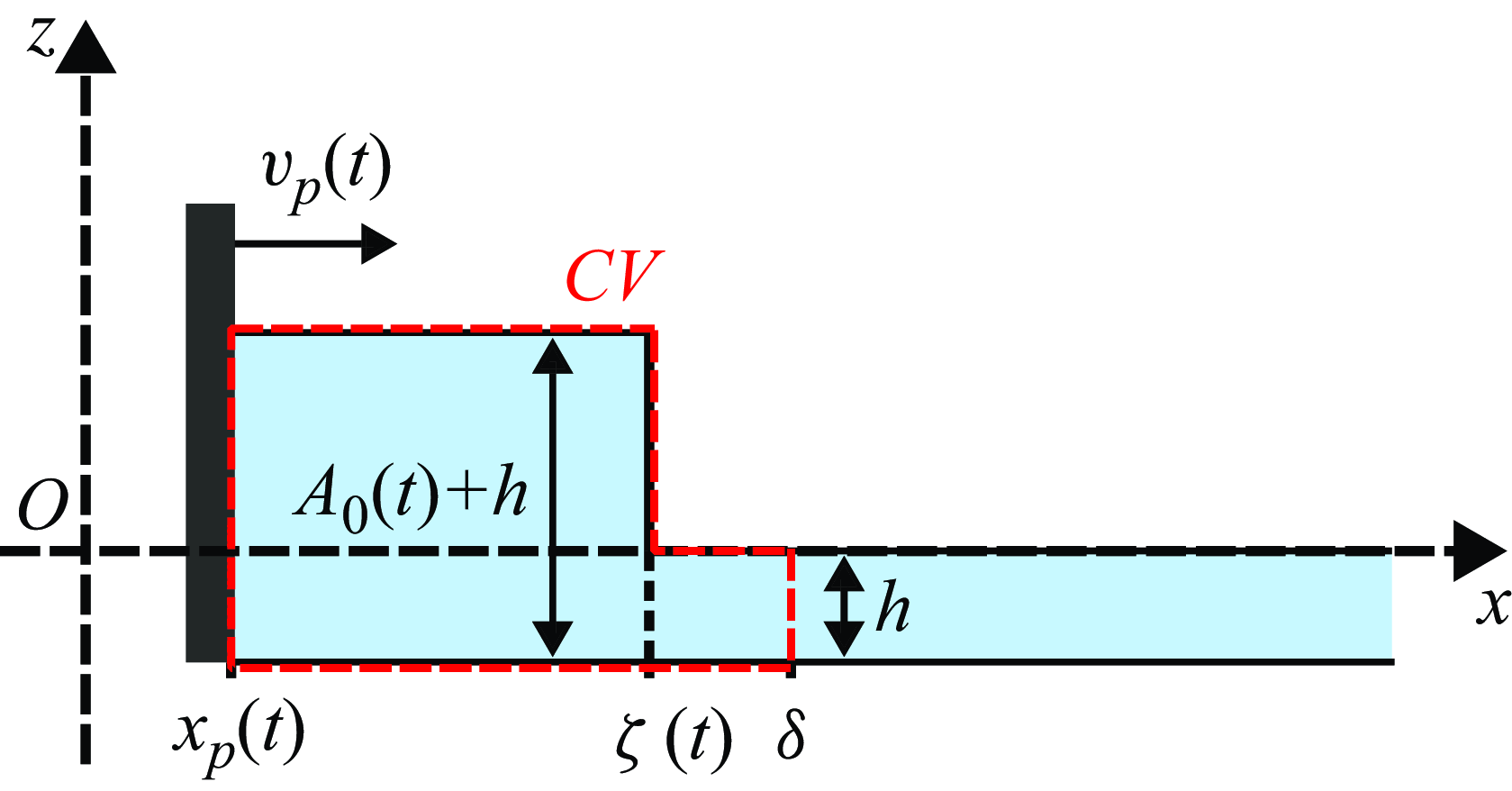
Schematic of an idealised transient hydraulic jump of upstream and downstream elevations $A_0(t) + h$ and $h$ , respectively. Here, $x_p(t)$ is the distance travelled by the piston at time $t$ , $v_p(t)$ its horizontal velocity, $\zeta (t)$ the location of the shock and $\delta$ the position of the shock at the end of the generation phase, i.e. $\delta \equiv \zeta (t=L/U)$ . The letters CV stands for control volume (per unit width), which is highlighted by the red contour.

5.2. Large Froude number: the unsteady hydraulic jump

As already discussed beforehand, non-linear effects induce a steepening of the wave near the end of the generation phase for large values of the Froude number $\mathrm {Fr}_p$ . This feature is pronounced for the plunging breaking bores and the water jets, as illustrated in figures 3(c) and 3(d). This observation is reminiscent of the formation of a hydrodynamic shock close to the source region, which is the response of the fluid to the impulse motion of the translating wall. To capture the physical mechanism at play in those circumstances, we consider the idealised case of a two-dimensional unsteady shock located at position $\zeta (t)$ at time $0 \lt t \lt L/U$ , which separates an upstream region of thickness $A_0(t)+h$ , for $x_p(t)\lt x\lt \zeta (t)$ , from another one of thickness $h$ located downstream, i.e. for which $x\gt \zeta (t)$ . Such a scenario is illustrated by the schematic shown in figure 8. It will be assumed here that (i) the flow is purely horizontal and invariant along the $z$ direction, that (ii) the fluid is inviscid and incompressible, and that (iii) the pressure can be considered as hydrostatic, i.e. $p(x,z,t)=\rho g [\eta (x,t) - z]$ . Conditions (i) and (iii) correspond to the shallow water approximation, which implies that the vertical acceleration of the fluid is neglected (Acheson Reference Acheson1990), and (ii) means that no dissipation occurs at the bottom of the flume during the bump formation. The fixed downstream position $\delta$ , indicated in figure 8 and corresponding to the right side of the control volume (CV), is chosen as the location of the shock along the $x$ axis at the end of the generation phase, i.e. $\delta \equiv \zeta (t=L/U)$ . Therefore, the volume of fluid comprised between the abscissa $x_p(t)$ and $\delta$ and between the altitudes $-h$ (bottom of the water tank) and $\eta (x,t)$ always contains the same water particles during the generation process. From a calculation detailed in Appendix A, the mass and horizontal momentum conservation equations applied to such an unsteady control volume read

(5.2) \begin{gather} \Bigl ( A_0(t) + h \Bigr ) \Bigl ( \dot {\zeta }(t) - v_p(t) \Bigr ) - h \dot {\zeta }(t) = 0, \end{gather}

(5.3) \begin{gather}\Bigl ( A_0(t) + h \Bigr ) \Bigl ( \dot {\zeta }(t) - v_p(t) \Bigr )^2 - h \dot {\zeta }(t)^2 + \frac {1}{2} g \Bigl ( \bigl ( A_0(t) + h \bigr )^2 - h^2 \Bigr ) = 0. \end{gather}

The combination of these two equations leads to the following non-linear relation between the instantaneous Froude number $\mathrm {Fr}(t)=v_p(t)/\sqrt {gh}$ and relative amplitude of the bore $A_0(t)$ :

(5.4) \begin{equation} \mathrm {Fr}(t) = \frac {A_{0}(t)}{h} \left (\frac {1 + A_{0}(t)/\left (2h\right )}{1 + A_{0}(t)/h}\right )^{1/2}. \end{equation}

Equation (5.4) constitutes a transient version of the classical bore relationship (Synolakis Reference Synolakis1989; Whitham Reference Whitham1999). Furthermore, a comparison between this expression and the prediction for a stationary hydraulic jump given by equation (1.3) reveals the quasi-static behaviour of the unsteady hydraulic jump. As this equation corresponds to a third-order equation for $A_0(t)/h$ , the only explicit expression for $A_0(t)/h$ as a function of Fr( $t$ ) which is physical is therefore

(5.5) \begin{equation} \begin{aligned}\frac {A_0(t)}{h}& =\frac {2}{3} \left \{ 2 \sqrt { 1 + 3 \mathrm {Fr}(t) ^2 /2 }\right.\\ & \quad \left. \cos\! \left ( \!\frac {1}{3} \cos ^{-1} \!\left [ \frac {3}{4}\frac { \left ( \mathrm {Fr}(t)-2\sqrt {2}/3 \right ) \left ( \mathrm {Fr}(t)+2\sqrt {2}/3 \right )}{ \left ( \mathrm {Fr}(t)^2+2/3 \right ) \sqrt { 1 + 3\mathrm {Fr}(t)^2 /2 }} \right ] \right ) - 1 \right \}\!. \end{aligned}\end{equation}

It should be emphasised that the equations (5.2)–(5.5) are obtained for the generation phase, i.e. when $tU/L \leqslant 1$ . Interestingly, as during this stage the piston velocity is $v_p(t)=U^2 t/L$ , equations (5.4) and (5.5) predict that the maximum amplitude $A_{m0}$ reached at $t=L/U$ is independent of the piston stroke $L$ .

Figure 9.

Wave amplitude $A_0$ at the contact with the piston as a function of the adjusted time $t^\prime$ , for the four experiments of figure 5. Only the generation phase is represented here and $t^\prime$ is defined as $t-t_0$ , where $t_0$ corresponds to the starting time of the generation process. The solid (–) and dashed (- - -) lines are the predictions given by equations (5.5) and (5.6), respectively. The symbols and their colours are the same as in figures 4(a)-(d).

In order to compare the outcomes of this modelling to the experiments, figure 9 displays the temporal evolution of $A_0$ during the generation phase for the four experiments of figure 5. In each plot, the solid line is the prediction given by the quasi-static hydraulic jump theory presented in this section, that is obtained by evaluating equation (5.5). The time $t^\prime$ corresponds to $t-t_0$ , where $t_0$ has been slightly adjusted for the experimental curves to initially coincide with the analytical ones, as the acquisition frequency of the camera ( $50\,\rm Hz$ ) did not allowed us to determine accurately the starting time of the generation process. Despite the strong underlying assumptions of the present modelling, there is a striking agreement between the theoretical predictions and the experimental water bumps that will eventually evolve to (c) a bore wave and (d) a water jet, for which the Froude number $\mathrm {Fr}_p$ is large ( $\mathrm {Fr}_p=2.0$ and $\mathrm {Fr}_p=2.2$ , respectively). More surprisingly, the prediction from equation (5.5) also captures the time evolution of the wave amplitude $A_0$ for the two cases leading to a dispersive wave (figure 9 a) and a solitary-like wave (figure 9 b), even if these regimes consist during their formation of a water bump that seems to be quite different from the idealised situation considered in figure 8. This suggests that the approach followed in § 5.2 remains valid for a large range of Froude numbers. In addition, the prediction

(5.6) \begin{equation} \frac {A_0(t)}{h} = \mathrm {Fr}(t) + \frac {1}{4} {\mathrm {Fr}^2(t)} \end{equation}

from Synolakis (Reference Synolakis1986, Reference Synolakis1989) is also reported in dashed line in figure 9(a–d). This law also exhibits good agreement with the measured values for the two low Froude number cases of figures 9(a) and 9(b), where it is almost indistinguishable from equation (5.5). However, the prediction from equation (1.2) slightly overestimates $A_0$ at the end of the generation phase for experiments featuring large values for the Froude number (figures 9 c and 9 d).

Figure 10.

Evolution of the relative maximum amplitude of the wave at the contact with the piston, $A_{m0}/h$ , as a function of the Froude number, $\mathrm {Fr}_p$ . The black solid line (—) corresponds to the quasi-static hydraulic jump prediction obtained by evaluating equation (5.5) at $t=L/U$ , the black dashed line ( $\hbox{-}\,\hbox{-}$ ) corresponds to equation (5.6) from Synolakis (Reference Synolakis1989), calculated at the same time, while the gray dash-dotted line () corresponds to equation (1.1) from Noda (Reference Noda1970). All experiments from the present study are reported, with the same symbols and colours as in figure 2(e), alongside data from Synolakis (Reference Synolakis1986, Reference Synolakis1989) ().

To further compare the experimental results with the different available models, the relative maximum amplitude of the wave at the contact with the piston, $A_{m0}/h$ , is shown as a function of the piston Froude number $\mathrm {Fr}_p$ in figure 10, for all the experiments performed in the present study. Regardless of the wave regime that is obtained after the generation process, all data collapse on a master curve, highlighting once more the strong link between $A_{m0}/h$ and $\mathrm {Fr}_p$ that has already been emphasised in several past studies (Noda Reference Noda1970; Das & Wiegel Reference Das and Wiegel1972; Fritz et al. Reference Fritz, Hager and Minor2004; Viroulet et al. Reference Viroulet, Cébron, Kimmoun and Kharif2013; Robbe-Saule et al. Reference Robbe-Saule, Morize, Henaff, Bertho, Sauret and Gondret2021b ; Sarlin et al. Reference Sarlin, Morize, Sauret and Gondret2021b , Reference Sarlin, Morize, Sauret and Gondret2022a ). As a corollary to this observation, there is no significant influence of the stroke $L$ of the piston on the value of $A_{m0}/h$ . The data from Synolakis (Reference Synolakis1986, Reference Synolakis1989), corresponding to three laws of motion for the piston (constant velocity, trajectory optimised for solitary wave generation and asymmetric parabolic trajectory), are also reported in figure 10 (). These measurements lie on the same trend as the experiments from the present study, which suggests that the relationship between $A_{m0}/h$ and $\mathrm {Fr}_p$ is robust and independent on the detail of the forcing in a wide range of Froude numbers. Furthermore, as the studies performed by Synolakis (Reference Synolakis1986, Reference Synolakis1989) involved a much larger tank as the one used here, this confirms that there is no significant effect of capillarity in the present experiments. The quasi-static hydraulic jump prediction, obtained by evaluating equation (5.5) at time $t=L/U$ , is also reported in figure 10 in black solid line. It closely matches the experimental measurements, especially for $\mathrm {Fr}_p \gtrsim 0.4$ , without any adjustable parameters. This further validates the approach of describing the generated waves as quasi-static shock waves. As equation (5.5) is obtained in the limit of large Froude numbers, experiments for which the shock is pronounced, i.e. (,) bore waves or () water jets, are better captured by the theoretical prediction than, for instance, () dispersive waves. The prediction given by equation (1.2) (which is equation (5.6) from Synolakis (Reference Synolakis1989) evaluated at time $t=L/U$ ), reported in black dashed line in figure 10, is almost superimposed with equation (5.5) when $\mathrm {Fr}_p \lesssim 0.8$ but slightly overestimates the generated wave height for the experiments at larger values of $\mathrm {Fr}_p$ . Furthermore, equation (1.1) obtained by Noda (Reference Noda1970) using the linear theory is also reported in figure 10 in gray dash-dotted line for comparison. Although it gives a good first order estimate of the relative maximum amplitude $A_{m0}/h$ , it can be observed that the quasi-static hydraulic jump theory gives a slightly better prediction when $\mathrm {Fr}_p \lesssim 0.7$ . For larger Froude numbers, the good agreement between the theory of Noda (Reference Noda1970) and the experimental measurements is surprising as there is no proper justification for using the linear theory anymore, given that non-linear effects then become dominant.

The successful comparison between the experiments and the analytical development presented in the present section thereby suggests that, during the generation process, the observed water bumps behave as quasi-static hydraulic jumps whose vertical heights at the contact with the piston are dictated by the wall velocity $v_p(t)$ and the initial fluid depth $h$ . This leads, at the end of the formation stage, to a maximum wave amplitude $A_{m0}$ which follows a weakly non-linear evolution with the Froude number $\mathrm {Fr}_p$ , as highlighted by the evaluation of equation (5.5) at time $t=L/U$ . From there, when the piston starts its deceleration, the water bump of height $A_{m0}$ relaxes into one of the different wave regimes reported in figure 2(a–d).