1 Introduction
Starting jets have received considerable attention in the recent past owing to their presence in many biological systems, from the propulsion of aquatic creatures (Anderson & Demont Reference Anderson and Demont2000; Dabiri Reference Dabiri2009) to the blood flow through the human heart (Kim et al. Reference Kim, Walker, Pedersen, Poulsen, Oyre, Houlind and Yoganathan1995; Kheradvar & Pedrizzetti Reference Kheradvar and Pedrizzetti2012; Pedrizzetti & Domenichini Reference Pedrizzetti and Domenichini2015). The fluid dynamics associated with starting jets makes it pertinent to study vortex rings and vortex pairs, since they are directly associated with starting jets. Studies in the recent past (Gharib, Rambod & Shariff Reference Gharib, Rambod and Shariff1998; Linden & Turner Reference Linden and Turner2004; Afanasyev Reference Afanasyev2006) have looked at vortex rings/pairs with the intent of better understanding these biological flows. Most of these biological systems, be it heart valves or the deforming mantle of a jellyfish, are composed of deformable membranes, and hence better understanding of these systems also requires an understanding of the interaction of such flows with deformable membranes, which is the focus of the present study. However, the configuration and parameters chosen for the present work do not represent any particular biological system. Instead, the chosen configuration of an idealized two-dimensional jet emanating from a channel with flexible flaps at the exit can be thought of as a model/simplified problem for understanding the effects of flexibility on flow generation for the more complex biological systems, and would also be of interest in pulsed jet based propulsion systems for use with underwater autonomous vehicles.
Developments in the study of aquatic propulsion mechanisms (Daniel Reference Daniel1983; Sahin, Mohseni & Colin Reference Sahin, Mohseni and Colin2009; Weston et al. Reference Weston, J. H., Costello and Abbott2009; Katija et al. Reference Katija, Colin, Costello and Jiang2015), especially unsteady jet propulsion by jellyfish, squids and salps have shown that a better understanding of starting jets can help us in gaining insight towards these systems. Dabiri et al. (Reference Dabiri, Gharib, Collin and Costello2005) for example, used dye visualization to look at the flow patterns in some species of jellyfish. They showed that the flow resembled the formation of vortex rings at different phases of its propulsion. Starting jets have also been observed in other aquatic creatures like squids and salps which use unsteady jets for propulsion. Anderson & Demont (Reference Anderson and Demont2000) made experimental measurements on squids to characterize the jet velocity and the jet thrust achieved by the squids during propulsion, highlighting the unsteady nature of the flow. More recently, Ruiz, Whittlesey & Dabiri (Reference Ruiz, Whittlesey and Dabiri2011) showed through direct measurements on a self-propelling body that the pulsed jet mode of propulsion was more efficient than the steady jet mode of propulsion. Whittlesey & Dabiri (Reference Whittlesey and Dabiri2013) conducted experiments using a self-propelled vehicle and found that the propulsive efficiency was also dependent on the vortex ring characteristics. They suggested that the optimal efficiency was linked with the vortex ring pinch off, which essentially means the time when the vortex ring has achieved its maximum circulation (Gharib et al. Reference Gharib, Rambod and Shariff1998). Dabiri (Reference Dabiri2009) provides a comprehensive review on the ‘optimal’ vortex formation across different biological systems. Kim, Hussain & Gharib (Reference Kim, Hussain and Gharib2013) studied the vortex dynamics of clapping plates and showed that the force generated by the plates is sensitive to the aspect ratio of the plates, with the impulse being larger for low aspect ratio plates, thus suggesting that low aspect ratio wings are more efficient for some modes of flapping flight. Studies (Gladfelter Reference Gladfelter1973; Shorten et al. Reference Shorten, Davenport, Seymour, Cross, Carrette, Woodward and Cross2005; Colin et al. Reference Colin, Costello, Katija, Seymour and Kiefer2013) have also looked at the kinematics of jellyfish velums, which are essentially thin membranes surrounding a body. The movement of these velums and how it relates with the flow generated can give us important clues regarding their benefits for propulsion. It was reported in the study by Dabiri, Colin & Costello (Reference Dabiri, Colin and Costello2006) that the velar kinematics of live jellyfish influences the formation of an optimal vortex structure. Gemmell et al. (Reference Gemmell, Costello, Colin, Stewart, Dabiri, Tafti and Priya2013) show that in a jellyfish, even the refilling phase which is essentially passive in nature leads to thrust production. This, they show using pressure calculations, happens because of a positive pressure created by a vortex ring that forms during the refilling phase.
The passive deformations of flexible portions of the body generating thrust has also received considerable attention recently with a large number of studies on flexible flapping plates and foils in particular (Michelin & Llewellyn Smith Reference Michelin and Llewellyn Smith2009; Spagnolie et al. Reference Spagnolie, Moret, Shelley and Zhang2010; Shelley & Zhang Reference Shelley and Zhang2011; Alben et al. Reference Alben, Witt, Baker, Anderson and Lauder2012; Quinn, Lauder & Smits Reference Quinn, Lauder and Smits2014a ,Reference Quinn, Lauder and Smits b ). For example, Marais et al. (Reference Marais, Thiria, Wesfreid and Godoy-Diana2012) in their flapping foil studies observed that by making the foil flexible in the chordwise direction, an average thrust of up to three times greater could be achieved when compared to rigid foils. In a computational study by Wilson & Eldredge (Reference Wilson and Eldredge2011), the effect of passively responsive components of a body was studied in the context of jellyfish using a two-dimensional jellyfish model comprised of linked rigid bodies with hinges modelled as torsional springs. They showed that such swimmers with passive hinges could swim faster and with better efficiency when compared to the actively controlled counterparts for a particular selection of torsional stiffness. Recently, Villanueva, Vlachos & Priya (Reference Villanueva, Vlachos and Priya2014) found that there exists a passive flap between the flexion point and the bell margin of a jellyfish. They suggest that there could be benefits in terms of efficiency with the presence of passive flexibility, by doing a comparative analysis of biomimetic robotic jellyfishes. Lucas et al. (Reference Lucas, Johnson, Beaulieu, Cathcart, Tirrell, Colin, Gemmell, Dabiri and Costello2014) compiled empirical data for the bending patterns of propulsors (e.g. fins or wings) across various animal sizes, fluid media and taxonomic groups. They show remarkable similarities across all animals when it comes to the propulsor bending patterns. They show that even though the propulsors may be actuated (birds, bats, fish, cetaceans and molluscs) or completely passive (insects), and their material properties are different, the similarities in their bending patterns remain consistent. This allows them to conjecture that bending kinematics may be fundamentally important for flexible biological propulsion.
In our previous study (Das, Govardhan & Arakeri Reference Das, Govardhan and Arakeri2013), we explored the effect that passive exit flexibility has on the formation process of a two dimensional starting jet by hinging two rigid flaps at the channel exit, with the hinge stiffness and damping being negligibly small. The starting jet was generated using a piston–channel mechanism that pushed fluid out of a high aspect ratio rectangular duct into a quiescent medium of the same fluid. The measurements showed that the introduction of flaps dramatically altered the flow with the generation of additional pairs of vortices that lead to a complete redistribution of vorticity compared to the rigid exit case. It was shown that the kinematics of the flaps across different flap lengths and jet speeds was largely governed by a non-dimensional time given by the ratio of the fluid slug length (
 $L$
) to the flap length (
 $L_{f}$
), and not the conventional one based on the exit width (
 $L/d$
,
 $d=\text{channel width}$
). The present study extends the previous work by introducing flexibility using deformable flaps that have an inherent flexural rigidity (
 $EI$
). This would be a step closer to biological systems which have membranes that deform as opposed to hinged-rigid flaps, and that in general possess some flexural rigidity.
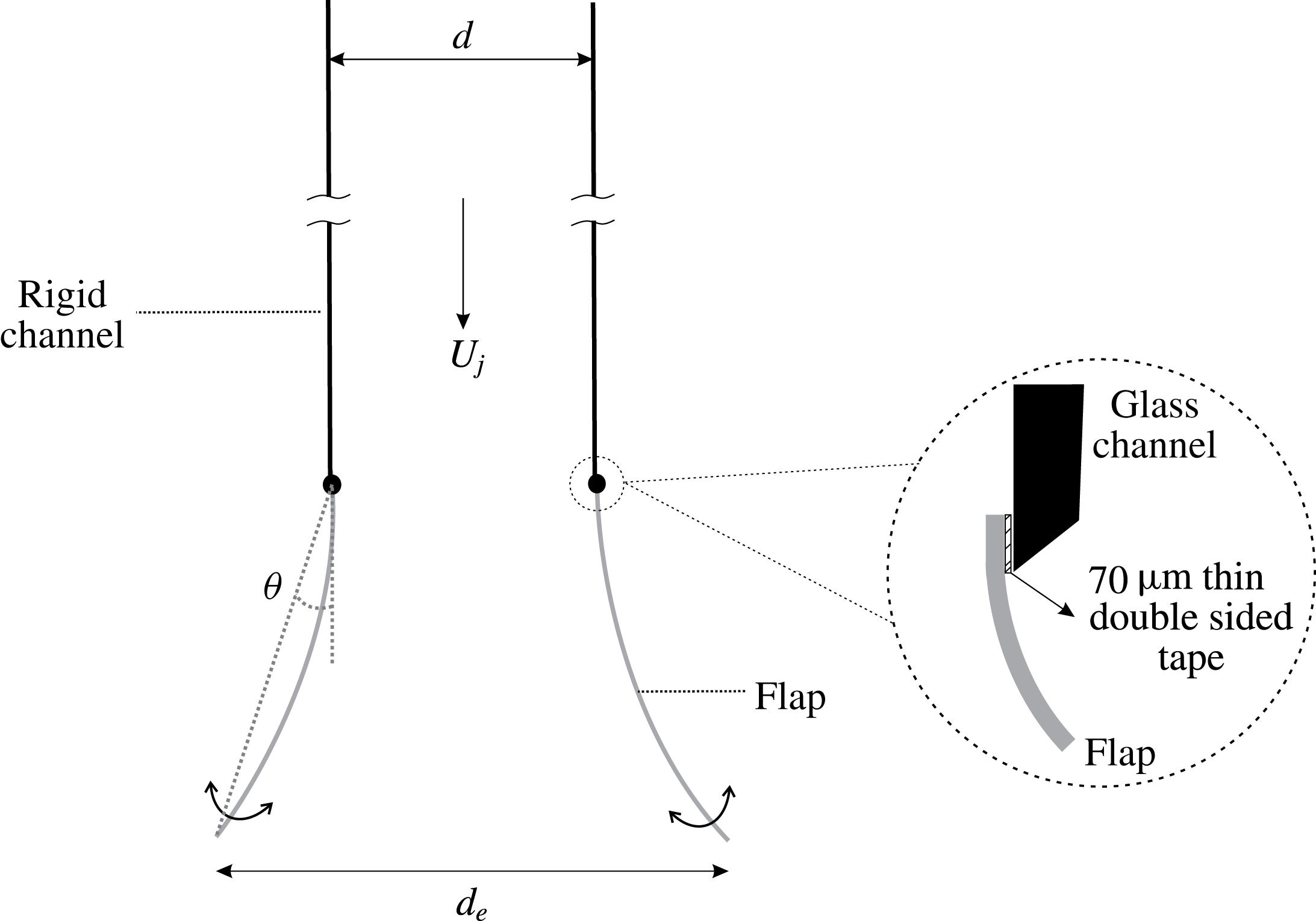
Schematic showing the arrangement used with deformable flaps or leaflets at the exit and the associated nomenclature. Here,
 $d$
is the channel width,
 $d_{e}$
is the exit width at flap tip that changes with time due to flap deformation,
 $U_{j}$
is the jet velocity (which is equivalent to the piston speed
 $U_{p}$
) and
 $L_{f}$
is the flap length.

In the present study, we introduce exit flexibility in the form of two flexible flaps placed at the exit of the nozzle of a two-dimensional starting jet (figure 1), with the main flap parameters being its streamwise length (
 $L_{f}$
) and its flexural rigidity (
 $EI$
). As in the study of Das et al. (Reference Das, Govardhan and Arakeri2013), the initial position of the flaps were set to be parallel to the channel walls. The starting jet was generated by a piston–cylinder mechanism, with the velocity profile of the piston being a rapid acceleration to a constant velocity (
 $U_{p}$
), followed by an impulsive stop, with the constant velocity phase being by far the longest. The flap length (
 $L_{f}$
) and its flexural rigidity (
 $EI$
) were varied along with the jet velocity (
 $U_{p}$
). Once the flow starts after the piston has been set into motion, the flap’s motion and the flow patterns hence generated were directly visualized, and flow field measurements were made using particle image velocimetry (PIV).
This paper is organized as follows. We present the details of experimental methods used in § 2. In § 3, we discuss the flap kinematics for all the cases studied and compare across different parameter variations. In § 4, we present the vorticity dynamics for the different flap cases and show how the presence of flaps could lead to desirable changes in terms of thrust production. In § 5, we present the conclusions from this study.
2 Experimental set-up
The work presented here was carried out in a free surface water tank of dimension
 $1~\text{m (length)}\times 1~\text{m (width)}\times 1.2~\text{m (depth)}$
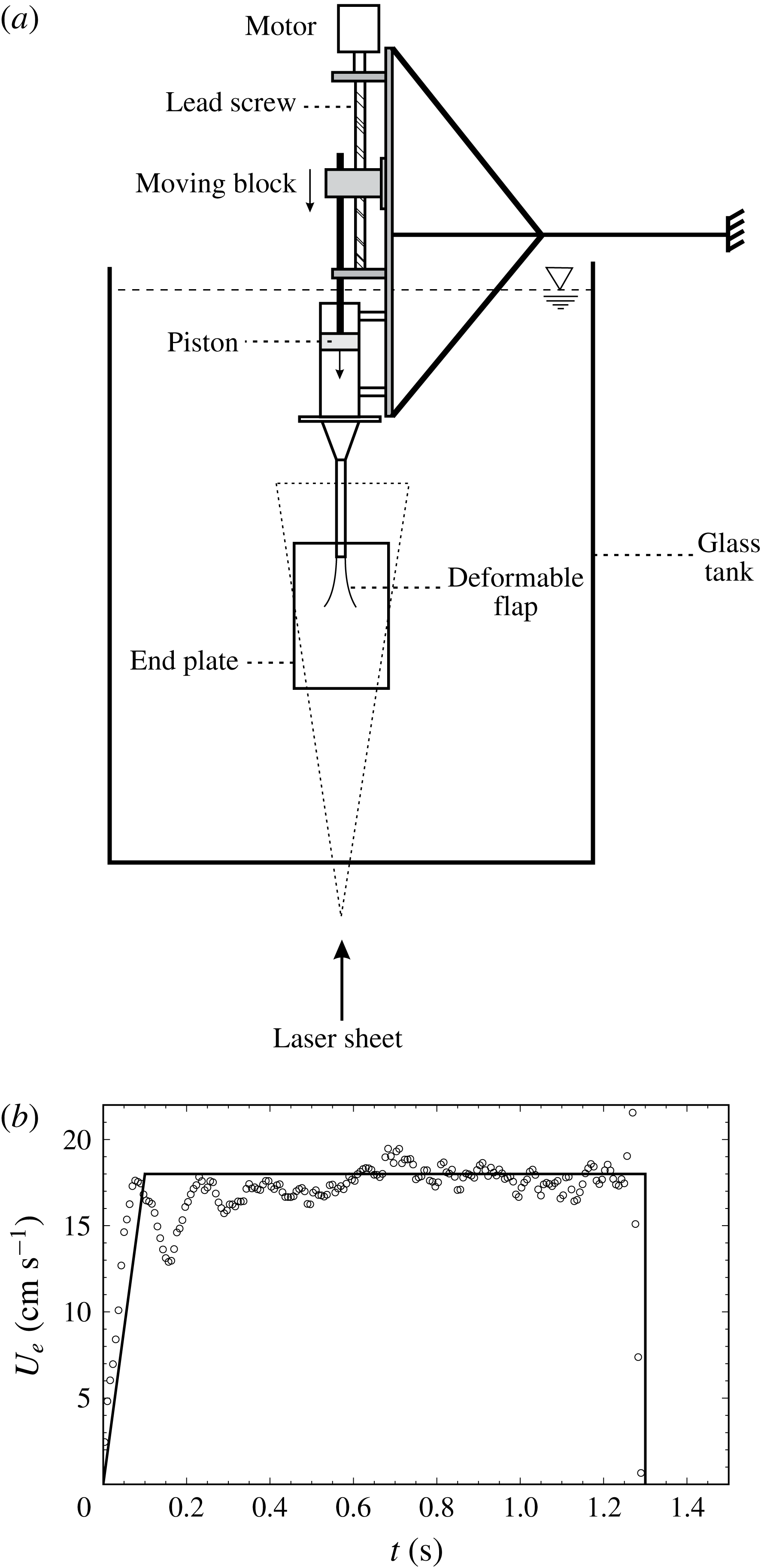
. The tank was built using 12 mm thick glass panels. A schematic of the experimental set-up including the starting jet generation mechanism and the water tank is shown in figure 2(a). The piston–cylinder mechanism used to generate the starting jet was directly bolted to a wall on one side to suppress any vibrations, without any contact with the water tank structure.
(a) Schematic of the experimental set-up used for the study with deformable flaps at the exit of the channel. (b) The measured channel exit velocity (
 $U_{e}$
) from PIV as a function of time (open circles), along with the desired velocity profile given to the piston (solid line) for a sample run.

The starting jet was generated by a piston–cylinder mechanism composed of a servo motor combined with a lead screw to drive the piston. The servo motor (Panasonic, A4 series) was controlled by a programmable logic controller (PLC), which could be programmed from a computer, enabling the piston motion profile to be controlled as desired. The piston was made using polypropylene material and was machined to fit inside a long rectangular duct with minimal clearance. The streamwise length of the piston was kept large at 55 mm compared to the channel width of 15 mm, to provide extra resistance to the fluid from leaking across the sides of the piston. The piston moved inside a stainless steel rectangular duct with cross-section of
 $300~\text{mm (span)}\times 35~\text{mm (width)}$
, which was then connected to a glass channel with cross-section of
 $300~\text{mm (span)}\times 15~\text{mm (width)}$
through a contraction. This large aspect ratio helped to promote two-dimensionality of the flow. The streamwise length of the glass channel was kept large at 250 mm compared to the channel width, so that any flow disturbances due to the contraction would not be pushed out of the channel for the fluid slug length (
 $L/d=15$
) studied. The glass channel was made using 5 mm thick glass panels and it was fitted with two end plates of dimensions
 $32~\text{cm}\times 23~\text{cm}$
, made using 4 mm thick Perspex sheets. End plates were used (figure 2) to promote two-dimensionality of the flow as in Das et al. (Reference Das, Govardhan and Arakeri2013). The flaps were attached to the channel using thin double sided tissue tape of
 $70~\unicode[STIX]{x03BC}\text{m}$
. The maximum thickness of the flaps used was
 ${\approx}0.2~\text{mm}$
, which is small compared to the channel width (
 $d$
) of 15 mm ensuring that there was no significant disturbance to the flow inside the channel by the introduction of the flaps.
The desired jet exit velocity profile with time was achieved by controlled motion of the piston. Since it is difficult to generate a truly impulsive start motion for the piston, we have used throughout this study a piston velocity profile which rapidly accelerates the piston to the desired velocity (
 $U_{p}$
) in 0.1 s, after which this velocity (
 $U_{p}$
) was held constant for some time, before it was impulsively brought to rest. To validate the piston motion profile, we used PIV to measure the jet velocity at the rigid nozzle exit. Due to the developing boundary layers on the channel walls, the exit velocity profile is non-uniform, and hence an average velocity was calculated at each time instant from the measured jet exit velocity profile, as done by Krieg & Mohseni (Reference Krieg and Mohseni2013) to validate piston motion. In figure 2(b), we plot this spatially averaged jet exit velocity as a function of time (open circle) for a sample piston motion profile, along with the desired profile given to the servo motor shown by the solid line. We can see that the measured jet exit velocity (
 $U_{e}$
) reasonably matches the desired profile, with some variations caused by perturbations in the piston motion, which are most evident at the rapid starting and stopping of the piston motion. Although there are temporal variations in
 $U_{e}$
, we will see later (figure 4 and others), that the deflected flap position with time is relatively smooth. This is related to the fact that the deflected flap position is an integral quantity and effectively averages out the temporal variations in jet exit velocity that occur at previous instants. To check repeatability between runs having the same piston velocity profile, uncertainty estimates in the deflected flap position are shown in figure 4 at every alternate data point, estimated from 5 different runs, indicating that the uncertainty or variation in piston motion and hence in flap kinematics between runs is relatively small.
The instantaneous velocity fields were measured using time resolved particle image velocimetry. For this technique, the fluid was seeded with silver coated spherical hollow glass particles (SH400S33) of
 $14~\unicode[STIX]{x03BC}\text{m}$
mean diameter (Potters Industries, USA). The centre plane of the two-dimensional starting jet was illuminated by a thin laser sheet. The laser sheet was generated using a 1 W continuous green laser and a cylindrical lens which converted the laser beam to a sheet (
 ${\approx}2{-}3~\text{mm}$
in thickness). This laser sheet was passed through the central plane of the starting jets near the nozzle to capture the two-dimensional flow. Images were captured using a 1 megapixel high speed camera (Phantom Miro 110), at frame rates in the range of 200–350 frames per second depending on the flow speed. The frame rate was chosen to obtain a maximum displacement of approximately 5–8 pixels of the illuminated seeding particles between subsequent images. It was also ensured that there was no streaking of the particle motion in the image by suitable choice of the camera exposure time. Subsequent images were then paired together for processing in Dynamic Studio (Dantec Dynamics) using the adaptive correlation method. The final interrogation box size used was either
 $16~\text{pixels}\times 16~\text{pixels}$
or
 $32~\text{pixels}\times 32~\text{pixels}$
(with a 50 % overlap) depending on the experimental conditions. The accuracy of the PIV velocity field was estimated to be approximately 1 % of the peak measured velocity, based on a sub-pixel accuracy of approximately 0.1 pixel (Raffel et al.
Reference Raffel, Willert, Wereley and Kompenhans2007). Vorticity was evaluated using a central difference scheme with second-order accuracy leading to uncertainty estimates of less than 10 % of the peak vorticity evaluated.
2.1 Stiffness of the deformable flaps
We used flaps with three different flexural rigidity (
 $EI$
) values, where
 $E$
is the Young’s modulus and
 $I$
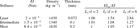
is the area moment of inertia of the flap. The flexural rigidity or stiffness of the flaps per unit span length and other details are listed in table 1. The flexural rigidity is an important parameter in our study, and we shall refer to the three values shown in table 1 often and hence in the rest of this paper we shall refer to the three
 $EI$
cases as least, intermediate and most stiff flaps. The span of the flaps used in our experiments was held constant at 30 cm that is equal to the span of the rectangular channel through which the starting jet ensues. The rectangular channel had a width (
 $d$
) of 1.5 cm. We used three different flap lengths (
 $L_{f}$
) of 3 cm, 6 cm and 9 cm, corresponding to (
 $L_{f}/d$
) values of 2, 4 and 6, respectively.
The details of the flap materials used in this study.

The flaps used were heavier than the fluid medium with specific gravities ranging from 1.3 to 1.6, and were mounted in a vertical configuration (figure 1). This implies that the net downward gravitational force (after subtracting buoyancy) experienced by the flaps would cause an additional restoring moment as the flaps open outward, in addition to the restoring moment due to the flexural rigidity (
 $EI$
) of the flaps. The net gravitational force acts as a uniformly distributed load on the flap (beam) trying to bring it back to its initial position, and a precise solution to such a problem is quite complicated and involves integro-differential equations. However, we can get a reasonable estimate for the increase in
 $EI$
caused by the net downward gravitational force by considering tip deflection of the flap modelled as a rigid beam with a torsional stiffness at the hinge point representing the restoring effect of flexural rigidity. With this simplification, it is easy to see that the net downward gravitational force acting at the mid-point of the flap would cause an increased restoring moment, which can in turn be written in terms of a higher equivalent flexural rigidity (
 $EI_{eq}$
) given by
 $EI_{eq}=EI(1+F_{g}{L_{f}}^{2}/(6EI))$
, where
 $F_{g}$
is the net downward gravitational force per unit span length of the flap after subtracting the buoyancy force. The values of the ratio of this equivalent flexural rigidity (
 $EI_{eq}$
) to the actual
 $EI$
are listed in table 1 for all the different
 $EI$
and flap length (
 $L_{f}/d$
) cases studied. It is clear from the table that the variations in
 $EI_{eq}$
from
 $EI$
are very small for the most and intermediate stiff flaps, and are significant only for the least stiff flaps, and in particular for the longer (
 $L_{f}/d=4$
and 6) least stiff flap cases.
The parameters involved in the study with deformable flaps can be noted from figure 1. The channel width (
 $d=1.5~\text{cm}$
) was kept constant throughout this work. The flap length (
 $L_{f}$
) is non-dimensionalized with the channel exit width (
 $L_{f}/d$
) and three different lengths,
 $L_{f}/d=2$
, 4, and 6 were studied. The instantaneous exit width at the flap tips is measured as
 $d_{e}$
. The flexural rigidity of the flaps (
 $EI$
) is a parameter, and we studied three flaps, each with a different
 $EI$
value (table 1). The fluid slug length (
 $L/d$
) is defined as the normalized streamwise distance moved by the fluid if the fluid moved as a slug. We have kept the final fluid slug length (
 $L/d$
) to be a constant at 15 in all the cases studied. The piston velocity program used was an impulsively started piston motion. For our experiments, we have used five different piston speeds between
 $10$
and
 $25~\text{cm}~\text{s}^{-1}$
giving us a Reynolds number (
 $Re=(U_{p}d)/\unicode[STIX]{x1D708}$
) range of 1500–3750. The dimensional time at which the piston stops is referred to as
 $\unicode[STIX]{x1D70F}$
hereafter, and the value of
 $\unicode[STIX]{x1D70F}$
varies with piston speed to keep
 $L/d$
constant at 15.
3 Flexible flap kinematics
In this section, we present the flap kinematics data for the cases studied. These include changes in the piston velocity (
 $U_{p}$
), the flexural rigidity (
 $EI$
) of the flaps and the length of the flaps (
 $L_{f}$
). Before each experiment, the flaps were kept parallel to the channel walls. As the flow was initiated, the flaps moved as dictated by the fluid forces along with forces due to flap stiffness and gravity. With these different parameters, we shall give an overview of the flap kinematics in this section.
3.1 Flap kinematics for a sample case
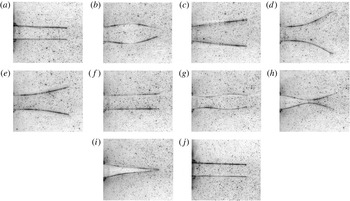
We begin by presenting in figure 3, a typical sequence of the flap kinematics visualized with time corresponding to the least stiff flap with
 $L_{f}/d=4$
and a piston velocity (
 $U_{p}$
) of
 $18~\text{cm}~\text{s}^{-1}$
. As the flow starts, the flaps bulge outwards (in a) due to an over-pressure that is developed in the flap region to accelerate the fluid slug contained between the flaps. This was also responsible for the opening out of the hinged rigid flaps in the study of Das et al. (Reference Das, Govardhan and Arakeri2013). However, since the flaps are deformable here, this excess pressure results in a local bulge as in figure 3(b). With time, this bulge is seen to grow and move downstream with the flow, leading to the opening outwards of the flap tip (figure 3
c) and ultimately resulting in the flap tips opening to a maximum value/extent in figure 3(d). Thereafter, the flaps gradually return to their initial position (figure 3
f). It should be noted that the piston accelerates rapidly from rest and reaches a steady speed before the maximum bulge is seen in figure 3(b). The inward motion of the flaps after their maximum opening can be attributed to two broad reasons, namely, the stiffness (
 $EI$
) of the flaps and to the lower pressure created in the flap region due to the ‘velocity head’ developed, the latter being similar to the reasoning made in Das et al. (Reference Das, Govardhan and Arakeri2013). Immediately after the piston is stopped (
 $t=\unicode[STIX]{x1D70F}$
), corresponding to a fluid slug length of 15, an under-pressure is developed within the flap region leading to the inward deflection of the flaps seen in figure 3(g) at
 $t/\unicode[STIX]{x1D70F}\approx 1.03$
. This under-pressure within the flaps is the opposite effect of the over-pressure seen at flow initiation, and is caused by the rapid deceleration of the flow between the flaps. This under-pressure leads to the inward deflection of the flaps that grows with time leading to the two flaps approaching each other (figure 3
h) and ultimately to the closure of the flaps with the tips touching each other (figure 3
i). This closure of the flaps by the under-pressure is similar to the observation of Lee & Talbot (Reference Lee and Talbot1979), who showed that an adverse pressure gradient due to fluid deceleration was the dominant reason behind closure of heart valves. As time progresses further, the flaps gradually open out to their initial position (figure 3
j).
Sequence of images showing the kinematics of the least stiff flaps with
 $L_{f}/d=4$
. The piston velocity program is impulsively started with
 $U_{p}=18~\text{cm}~\text{s}^{-1}$
, and sets up the flow that is from left to right. The piston stops at
 $\unicode[STIX]{x1D70F}\approx 1.3~\text{s}$
and the corresponding fluid slug length reached is
 $L/d=15$
. The instances shown in the figure are at
 $t/\unicode[STIX]{x1D70F}=$
(a) 0 (b) 0.1 (c) 0.19 (d) 0.28 (e) 0.59 (f) 0.97 (g) 1.03 (h) 1.1 (i) 1.16 (j) 4.8.

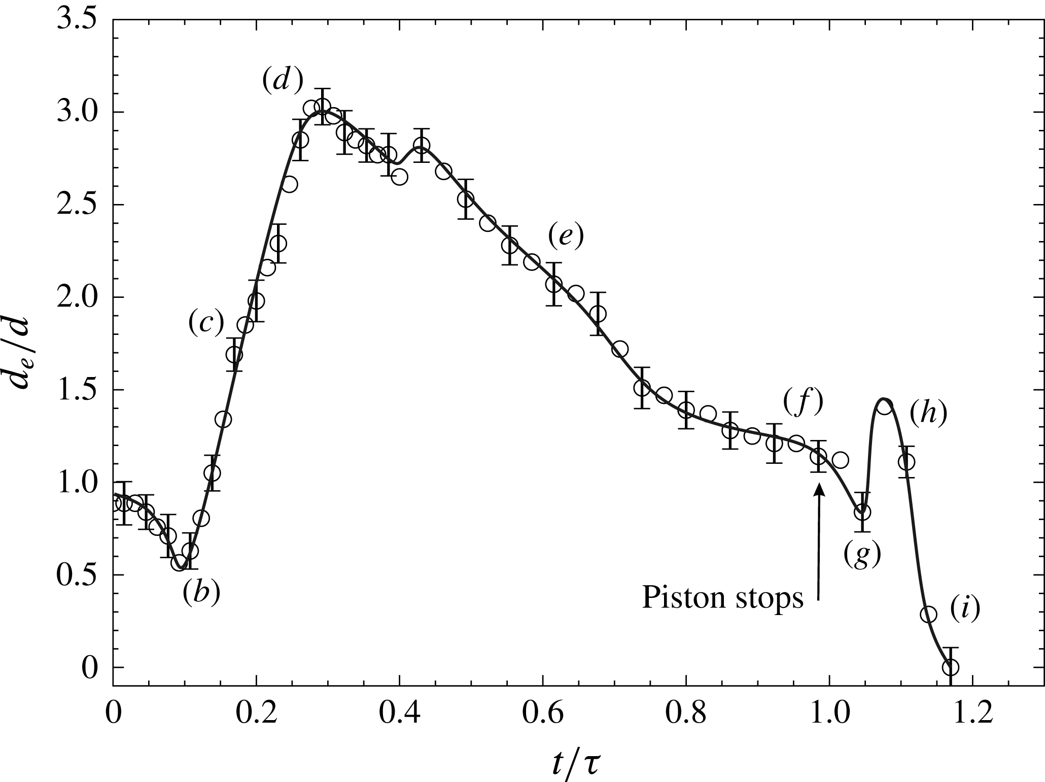
Plot of exit width with time for the least stiff flap and
 $L_{f}/d=4$
. The instances (b–i) are the same as shown in figure 3 with all other parameters being the same. The solid line is a trend line drawn for clarity and uncertainty estimates are shown at every alternate measurement point.

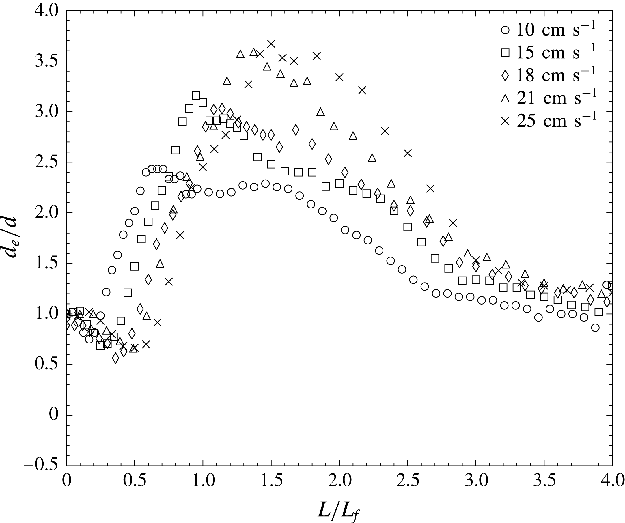
Plot of exit width with
 $L/L_{f}$
for varying piston speeds (
 $U_{p}$
). In all cases, the flap length (
 $L_{f}/d$
) is 4, the flaps are of least stiffness and the piston stops when the fluid slug length reaches
 $L/d=15$
.

In Das et al. (Reference Das, Govardhan and Arakeri2013), we used the rigid leaflet’s angle with respect to the channel walls to compare different cases and to study the leaflet kinematics. In the cases with deformable leaflets, however, there is no clear angle because the flaps deform. We therefore start with plotting the exit width based on flap tips (
 $d_{e}$
from figure 1) to look at the flap kinematics as a function of time. We present time variation of the exit width (
 $d_{e}$
) at the flap tips normalized by the channel width (
 $d$
) in figure 4, for the same case as in figure 3. The piston motion is nearly impulsively started to
 $18~\text{cm}~\text{s}^{-1}$
. The different instances (b–i) marked in the figure are the same instances for which the flap shapes are shown in figure 3. The uncertainty estimates in every alternate data point are shown in the figure, and are obtained from multiple runs of the same case. The initial streamwise central bulging of the flaps results in a reduction of the exit width (
 $d_{e}$
) as seen in the plot in figure 3(b). Thereafter the flap tips move out to reach the maximum exit width as shown in figure 3(d). The collapse of the flaps after the piston stops is reflected by a rise in the exit width (figure 3
h) as the tips move outwards, followed by a relatively fast coming together of the flaps resulting in the exit width reaching zero (figure 3
i).
We next show the kinematics for different piston speeds (figure 5) keeping the flap length constant at
 $L_{f}/d=4$
and employing the flaps of least stiffness. We have thus far presented the kinematics as a function of a simple non-dimensional time (
 $t/\unicode[STIX]{x1D70F}$
), where
 $\unicode[STIX]{x1D70F}$
is the time when the piston stops. This choice was deliberately made to permit discussions of flap kinematics even after the piston stops (
 $t/\unicode[STIX]{x1D70F}>1$
). The conventional time scale in such starting jet studies is the fluid slug length (
 $L$
), which is more relevant while the fluid is being pushed out, but remains constant once the piston stops, and hence is not convenient to discuss flap kinematics after the piston stops. However, hereafter we will be predominantly looking at the kinematics while the piston is in motion, and so we shall use the conventional fluid slug length (
 $L$
) as the non-dimensional time. In the study with hinged leaflets (Das et al.
Reference Das, Govardhan and Arakeri2013), we found that a time scale based on the fluid slug length and flap length (
 $L/L_{f}$
) collapsed the flap kinematics across different piston speeds (
 $U_{p}$
) and flap lengths (
 $L_{f}/d$
), where
 $L$
is the streamwise distance moved by the fluid if it moved as a slug. We therefore plot the kinematics for the different
 $U_{p}$
cases from this study using
 $L/L_{f}$
as the time scale in figure 5. In the present case of flexible flaps, we can clearly see changes in the exit width (
 $d_{e}$
) with
 $U_{p}$
, noting that the observed changes are significant compared to the uncertainty in
 $d_{e}$
shown in figure 4. This suggests that unlike in the hinged rigid flap study, the piston speed (
 $U_{p}$
) does influence the flap kinematics significantly. We shall address this aspect later in the section by defining an appropriate non-dimensional flexural rigidity (
 $EI^{\ast }$
) using both the flap stiffness (
 $EI$
) and
 $U_{p}$
, to capture this effect. We shall see that to a reasonable extent increasing values of
 $U_{p}$
may be seen as leading to a decrease in
 $EI^{\ast }$
, and hence an increase in the maximum observed flap opening. We shall explore this further after presenting results for varying flap lengths and stiffnesses in the following subsections.
Broadly, across all flap stiffness and lengths studied, we observe the features described above. However, the time scales and the extent of opening and closing can be very different as we vary the stiffness and length. This also implies that the flow dynamics (to be discussed in § 4) is different for each case. We shall now look at the flap kinematics for all the different cases systematically. We will make comparisons across different cases and try to explain the underlying reasons behind the observations.
3.2 Effect of flap stiffness and length on flap kinematics
We have used flaps with three different stiffness values (
 $EI$
) with three different flap lengths (
 $L_{f}/d$
) for each flap stiffness. We shall first present measured flap shapes as a function of time for different flap
 $EI$
values followed by different
 $L_{f}/d$
values. In all cases shown we keep the piston speed
 $U_{p}$
fixed at
 $18~\text{cm}~\text{s}^{-1}$
, as in the sample case shown earlier, for ease of understanding. The effects of
 $U_{p}$
will be presented separately later in the section.
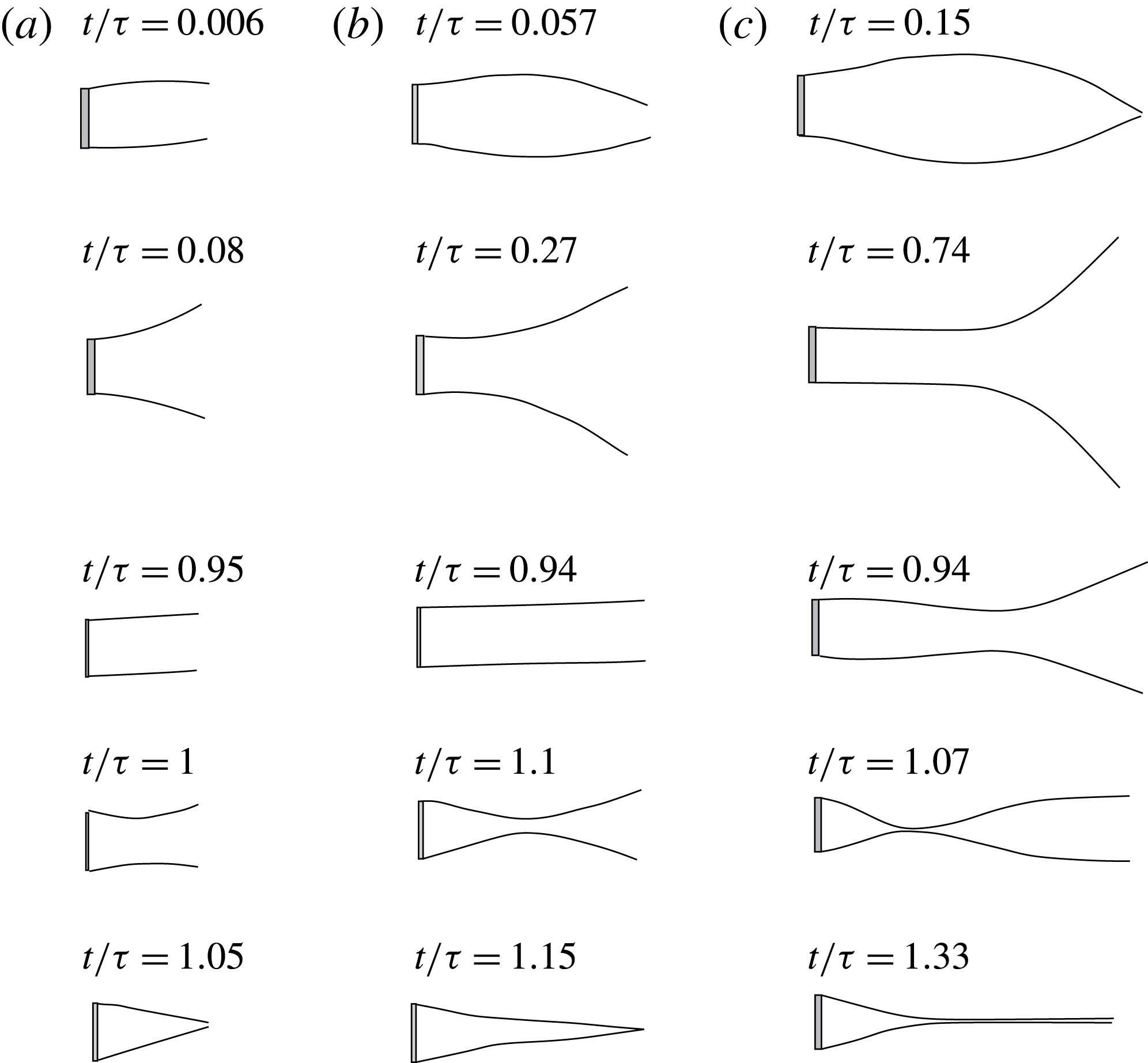
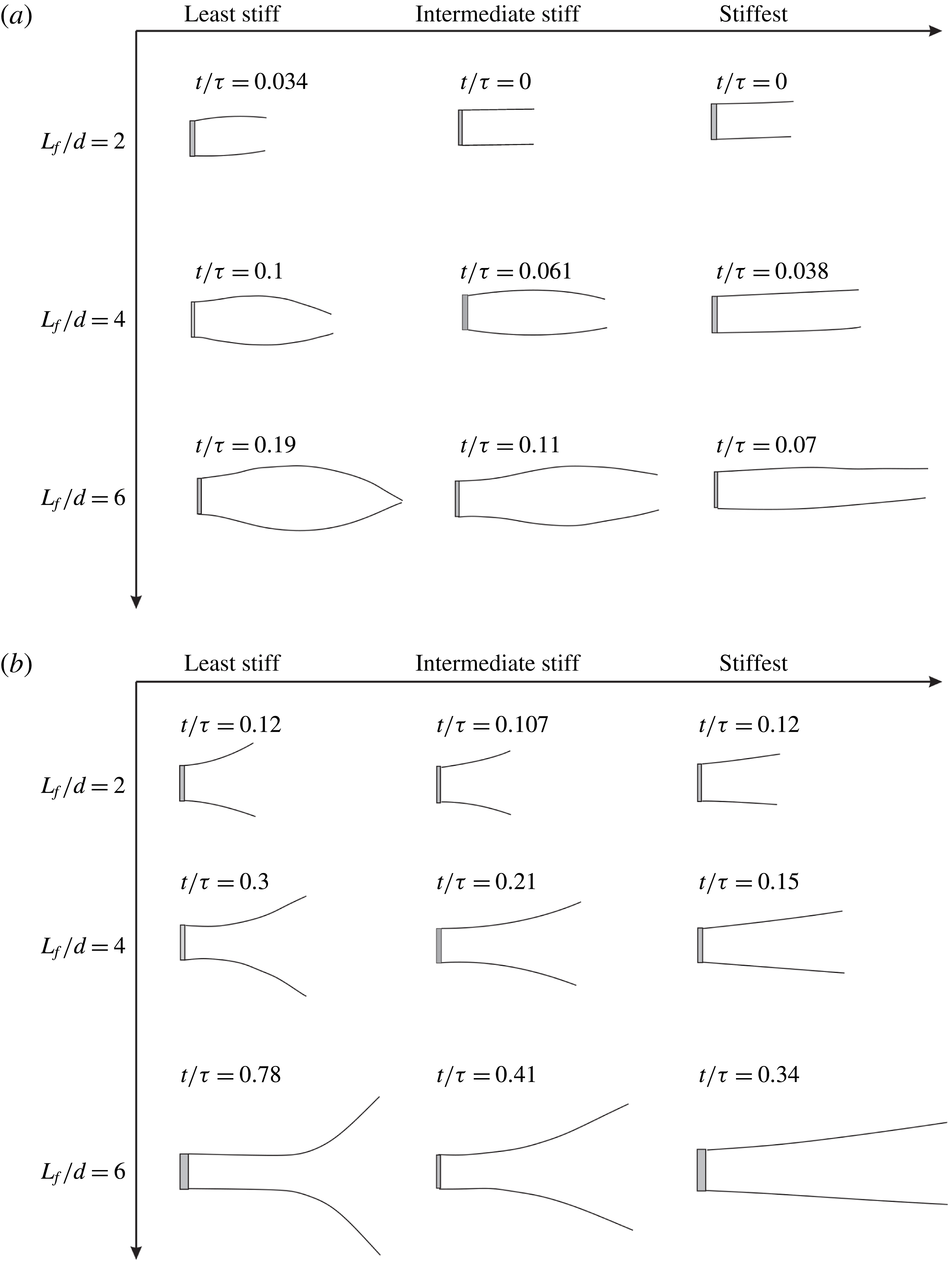
We first show the time sequence of flap kinematics for different stiffness values (
 $EI$
) in figure 6 keeping the flap length (
 $L_{f}/d$
) fixed at 4, as in the sample case already discussed. In each of the three stiffness cases shown, the instances correspond to flaps at the maximum bulge (minimum
 $d_{e}$
at flow initiation), maximum opening of the flap tips, just before the piston stops, immediately after the piston stops and the minimum
 $d_{e}$
reached after the piston stops. We chose these physical events, rather than a specific non-dimensional time, as none of the common non-dimensional time scales based on the piston velocity profile such as
 $t/\unicode[STIX]{x1D70F}$
or
 $L/L_{f}$
collapse these physical events across the different flap stiffness and length cases studied. This is contrary to our previous study (Das et al.
Reference Das, Govardhan and Arakeri2013) without stiffness, where the piston velocity based time scale,
 $L/L_{f}$
, was sufficient to collapse the data across different flap lengths. In addition, we have also tried to collapse the data using non-dimensional time based on the flap stiffness (
 $t/\sqrt{(\unicode[STIX]{x1D70C}L_{f}^{5}/EI)}$
) (Das Reference Das2016), this being the relaxation time scale for a flap with flexural rigidity (
 $EI$
) and with inertia that is dominated by fluid inertia (negligible mass flap as in the present case). However, even this flap stiffness based time scale did not collapse the flap kinematic data as shown in Das (Reference Das2016), highlighting the fact that there are competing time scales in the present problem, which makes the dynamics richer than in our previous study (Das et al.
Reference Das, Govardhan and Arakeri2013) that was in the absence of stiffness. As noted above, the instances corresponding to these physical events occur at different non-dimensional times (say
 $t/\unicode[STIX]{x1D70F}$
) for each of the cases, and the corresponding values of (
 $t/\unicode[STIX]{x1D70F}$
) are given in the figure. We can see from the figure that as the flap stiffness is increased, as one would expect, the maximum flap tip displacements reduce, and the changes in deflections are more gradual along the length of the flaps. The latter are especially clear at flow initiation (first image in each sequence) and immediately after the piston stops (fourth image in sequence).
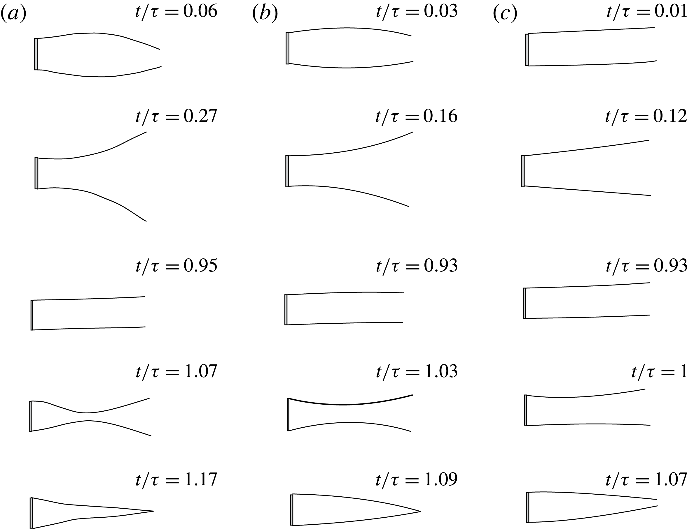
The effect of flap length (
 $L_{f}/d$
) on the flap kinematics is shown in figure 7 with the flap stiffness being maintained at the lowest value in all cases. The physical events or instances that we have selected to show are the same as in the previous figure. Although the
 $EI$
values are the same, we can see that larger flap lengths decrease the effective stiffness of the flap with longer flaps showing larger flap tip displacements, and larger variations in deformations along the flap length. As in the previous figure, the latter point is clear in the second and fourth images of the sequence for each case that shows the flap deformation at flow initiation and just after the piston stops. In particular, when the piston stops, the longer flap case (
 $L_{f}/d=6$
) shows a clear coming together of the two flaps at approximately 30 % of the flap length. Subsequently, the two flaps collapse and touch each other along a large fraction of the flap length as seen in the final image of the sequence for the longest flap case. This clearly highlights the fact that the total amount of fluid ejected in forming the starting jet can be significantly more than the case with no flaps. This is because some of the fluid from the flap region is expelled in addition to the amount of fluid pushed by the piston, the former effect being absent if there were no flaps. Thus, the net mass of fluid forming the jet is larger in the flap cases, although the same amount of fluid is pushed by the piston. We shall discuss this point in more detail in the next section. An overview of the flap deformation shapes for all the different flap stiffness values and lengths studied at four key instances in time corresponding to the maximum bulge, maximum opening, just after piston stops and when the flaps close fully is shown in the Appendix.
Flap deformation profiles with time for different flap stiffness values corresponding to (a) least stiff, (b) intermediate stiffness and (c) stiffest. In all cases,
 $L_{f}/d=4$
,
 $U_{p}=18~\text{cm}~\text{s}^{-1}$
and the piston stops at
 $\unicode[STIX]{x1D70F}=1.3~\text{s}$
corresponding to a fluid slug length (
 $L_{d}$
) of 15. The five time instances shown are the maximum bulge, maximum opening of the flap tips, just before the piston stops, immediately after piston stops and the final closing of the flap tips.

Flap deformation profiles with time for different flap length values corresponding to (a)
 $L_{f}/d=2$
, (b)
 $L_{f}/d=4$
and (c)
 $L_{f}/d=6$
. In all cases, the flaps are of least stiffness,
 $U_{p}=18~\text{cm}~\text{s}^{-1}$
, and the piston stops at
 $\unicode[STIX]{x1D70F}=1.3~\text{s}$
corresponding to a fluid slug length (
 $L_{d}$
) of 15. The five time instances shown are the maximum bulge, maximum opening of the flap tips, just before the piston stops, immediately after piston stops and the final closing of the flap tips.

Plot of exit width (
 $d_{e}/d$
) with
 $L/L_{f}$
. In (a), the stiffness (
 $EI$
) of the flap is varied while keeping the flap length fixed at
 $L_{f}/d=4$
, while in (b), the flap length (
 $L_{f}/d$
) is varied while keeping
 $EI$
fixed at the least stiffness value. In both cases, the piston velocity (
 $U_{p}$
) is
 $18~\text{cm}~\text{s}^{-1}$
, and the piston is stopped when the fluid slug length reaches
 $L/d=15$
.

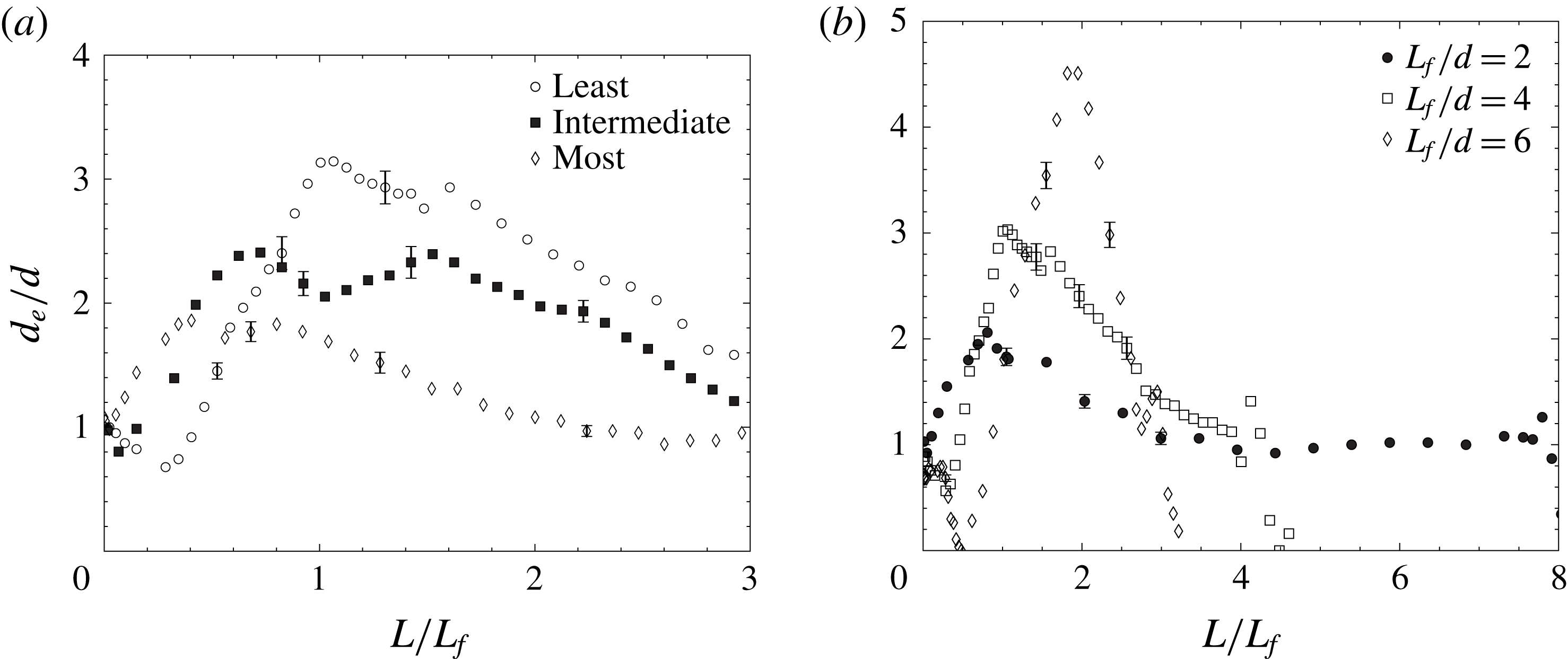
In figure 8, we plot the exit width as a function of (
 $L/L_{f}$
) for the different flap stiffness and flap length cases shown in the preceding two figures. Figure 8(a) shows the effect of variation in flap stiffness for the
 $L_{f}/d=4$
case, whereas figure 8(b) shows the effect of variation in flap length for the least stiff flap case. Both the plots show that there are significant variations in the flap kinematics with varying flap stiffness and flap length. It may also be noted that the changes due to these parameter variations are significantly larger than the uncertainties in measurement, which are shown at representative points in each plot. Further, as noted earlier, it is clear from these plots that physical events like maximum flap tip opening do not collapse when using the piston velocity profile based non-dimensional time scale
 $L/L_{f}$
. Other time scales, such as a flap stiffness based time scale (
 $t/\sqrt{(\unicode[STIX]{x1D70C}L_{f}^{5}/EI)}$
), also do not show collapse of the data (Das Reference Das2016). It is also clear, as shown earlier (figure 5), that the flap kinematics is also significantly affected by the piston velocity (
 $U_{p}$
). This is contrary to what was observed in the hinged leaflet cases of Das et al. (Reference Das, Govardhan and Arakeri2013), where a time scale based on (
 $L/L_{f}$
) collapsed the kinematics across different flap lengths and piston speeds. The differences in the flap motion observed in these figures clearly indicates that the flexural rigidity of the flaps (
 $EI$
), flap length (
 $L_{f}/d$
) and piston speed (
 $U_{p}$
) are all important in determining the kinematics of the flaps. This naturally raises the question of finding alternate non-dimensional parameters for the flap kinematics in the present case that should necessarily include
 $EI$
besides
 $L_{f}/d$
and
 $U_{p}$
.
With a view to finding alternate non-dimensional parameters involving
 $EI$
, we look at non-dimensionalized forms of flexural rigidity (
 $EI$
) used in the literature. Non-dimensionalized forms of flexural rigidity (
 $EI$
) have been used in other studies related to flag flutter (Connell & Yue Reference Connell and Yue2007), flexible flaps in the wake of a cylinder (Shukla, Govardhan & Arakeri Reference Shukla, Govardhan and Arakeri2013) or flapping foils (Shinde & Arakeri Reference Shinde and Arakeri2014). In our problem, the energy of the fluid coming out of the channel (
 $1/2\unicode[STIX]{x1D70C}dL_{f}U_{p}^{2}$
) can be expected to be of the same order as that of the energy stored by the flaps in the form of its bending stiffness (
 ${\sim}\unicode[STIX]{x1D6FF}^{2}EI/L_{f}^{3}$
, where
 $\unicode[STIX]{x1D6FF}$
is the flap tip deflection due to fluid forces). If we define a non-dimensional flexural rigidity as the ratio
 $L_{f}^{2}/\unicode[STIX]{x1D6FF}^{2}$
, then we get
 $$\begin{eqnarray}\displaystyle & EI^{\ast }={\displaystyle \frac{EI_{eq}}{{\displaystyle \frac{1}{2}}\unicode[STIX]{x1D70C}U_{p}^{2}L_{f}^{2}d}}, & \displaystyle\end{eqnarray}$$
where we have used
 $EI_{eq}$
, the equivalent flexural rigidity defined previously to take the self-weight of the flaps into account. The
 $EI^{\ast }$
defined here is slightly different from the previous studies of Connell & Yue (Reference Connell and Yue2007), Shukla et al. (Reference Shukla, Govardhan and Arakeri2013) and Shinde & Arakeri (Reference Shinde and Arakeri2014) that use (
 ${L_{f}}^{3}$
) in the denominator, while in the present definition we also have the channel width (
 $d$
) in the denominator which is a relevant parameter here.
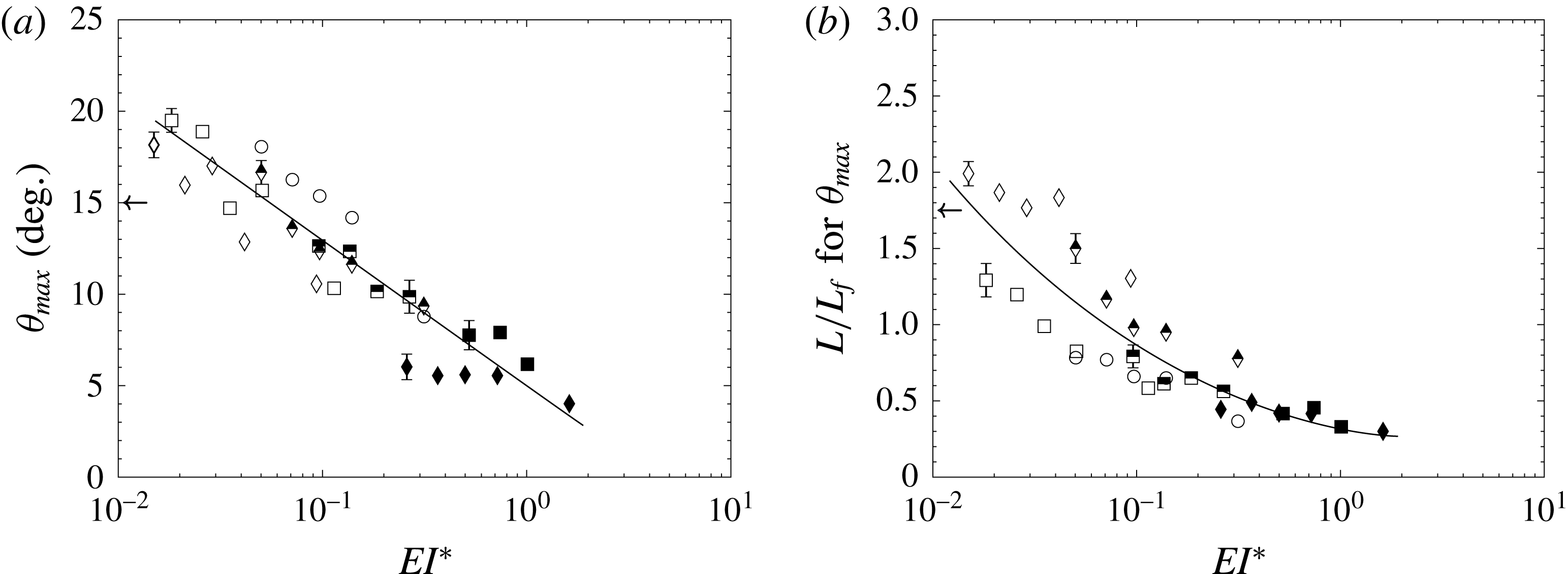
Plot of flap kinematic parameters from all experiments in the present study as a function of non-dimensional stiffness (
 $EI^{\ast }$
). The data shown here correspond to studies with different flap lengths (
 $L_{f}/d$
), flap stiffness values (
 $EI$
) and piston velocities (
 $U_{p}$
). In (a), the maximum tip based angle (
 $\unicode[STIX]{x1D703}_{max}$
) is shown, while in (b), the non-dimensional time (
 $L/L_{f}$
) required to reach the maximum
 $\unicode[STIX]{x1D703}_{max}$
is shown. The piston velocity program is impulsively started and the fluid slug length reaches
 $L/d=15$
in each case. The legends are: ○,
 $L_{f}/d=2$
; ▫,
 $L_{f}/d=4$
; ♢,
 $L_{f}/d=6$
; with open symbols for least stiff, half-filled for intermediate and filled for stiffest flaps. The arrows in both the panels represent the values for the hinged-rigid flap case of Das et al. (Reference Das, Govardhan and Arakeri2013), where the stiffness was close to zero.

We show that
 $EI^{\ast }$
is a useful non-dimensionalization in our experiments by directly plotting some overview parameters representing the flap kinematics against this non-dimensional parameter. Two such overview parameters representing flap kinematics could be the maximum flap tip opening and the time taken by the flap tips to reach that maximum opening. As noted before, in the present case, we do not have a unique angle because the flaps deform. However, we can define an angle
 $\unicode[STIX]{x1D703}$
based on a line joining the flap tip to the rigid end where the flap is fixed (as shown in figure 1). This angle
 $\unicode[STIX]{x1D703}$
is useful in making a broad comparison with the hinged-rigid cases, while also capturing the exit width (
 $d_{e}$
) as it is directly related to
 $d_{e}$
(
 $\unicode[STIX]{x1D703}=\tan ^{-1}(0.5(d_{e}-d)/L_{f})$
). We show in figure 9, the maximum flap opening (
 $\unicode[STIX]{x1D703}_{max}$
) and the time taken to reach
 $\unicode[STIX]{x1D703}_{max}$
, for all the different experiments that we have done, which include variations in
 $EI$
,
 $L_{f}/d$
and
 $U_{p}$
, plotted with
 $EI^{\ast }$
. In figure 9(a), we show the maximum flap tip opening in terms of the angle (
 $\unicode[STIX]{x1D703}_{max}$
) defined above. It is clear that the data from all the different cases fall onto an approximately linear trend line (on the log plot) indicating a reasonably good collapse of the data with
 $EI^{\ast }$
. It should be noted here that the collapsed data include variations in
 $U_{p}$
and
 $L_{f}/d$
apart from
 $EI$
, and hence, indicate that as far as the maximum flap opening is concerned, increases in
 $U_{p}$
and
 $L_{f}/d$
may be interpreted as equivalent to a reduced
 $EI^{\ast }$
. Further, the figure shows that as
 $EI^{\ast }$
is increased, the maximum flap tip angle (
 $\unicode[STIX]{x1D703}_{max}$
) decreases from approximately
 $20^{\circ }$
at the lowest values of
 $EI^{\ast }$
and drops to approximately
 $5^{\circ }$
at the higher end of the
 $EI^{\ast }$
regime studied. It may be noted here that the largest
 $\unicode[STIX]{x1D703}_{max}$
values seen here (approximately
 $20^{\circ }$
) are comparable to, but slightly higher than, the maximum angles seen for the hinged-rigid flap case studied in Das et al. (Reference Das, Govardhan and Arakeri2013) (shown by the arrow in the figure) where there was no hinge stiffness. In the present case, we see that at low values of
 $EI^{\ast }$
the angles are comparable to that case, with the angles decreasing from those values as
 $EI^{\ast }$
is increased. This plot thus gives a reasonable idea of the extent of flap opening across a range of
 $EI$
,
 $L_{f}/d$
and
 $U_{p}$
values. As
 $EI^{\ast }$
is further decreased towards zero, one would expect that at some value of
 $EI^{\ast }$
, the maximum flap tip angle would saturate to a value, with further reductions in
 $EI^{\ast }$
not leading to an increase in flap opening. From the plot, it is not clear if this saturation has been reached. Figure 9(b) shows the time taken by the flaps in terms of (
 $L/L_{f}$
) to reach the maximum angle as a function of
 $EI^{\ast }$
. Although the collapse is not as good as in figure 9(a), we find that the data from all cases can be reasonably well represented by a single trend line in the plot. It may be noted that the variations seen in figure 9(b) around the broad trend line are not due to experimental uncertainties, which are small, as shown by the uncertainty bars in the figure at representative points. In the plot, we have indicated data for different flap stiffness cases with open/half-filled/filled symbols, while each flap length is indicated by a different symbol. A closer inspection of the data indicates that
 $EI^{\ast }$
is able to reasonably well collapse the data across different flap stiffnesses and piston speeds for each of the three flap lengths. However, the collapse of the data for different flap lengths is not as good, with the longer
 $L_{f}/d=6$
flap data showing a small but distinctly different trend from the smaller two flap lengths data. This is likely related to the presence of more complex flap mode shapes with large bending close to the flap tips in the longer
 $L_{f}/d=6$
flap case, as shown in figure 7. However, a broad trend line is shown for all the three flap length data sets to give an overview of the data across all flap lengths, stiffnesses and piston speeds. At low values of
 $EI^{\ast }$
, as in figure 9(b), we find a reasonably good agreement between the present results and the data for the hinged-rigid flap case studied in Das et al. (Reference Das, Govardhan and Arakeri2013), both showing
 $L/L_{f}$
values of approximately 1.75–2. As the
 $EI^{\ast }$
value is increased, the
 $L/L_{f}$
values corresponding to maximum
 $\unicode[STIX]{x1D703}_{max}$
drop down to approximately 0.5 at the highest
 $EI^{\ast }$
value studied of approximately 1. The reasonable collapse of the flap kinematics data with
 $EI^{\ast }$
indicates that
 $EI^{\ast }$
is a good normalization for flap stiffness, and can be used to broadly collapse data from a wide range of independent experiments covering variations in
 $EI$
,
 $L_{f}/d$
and
 $U_{p}$
.
4 Vortex dynamics
In this section, we present the vorticity dynamics of the unsteady jet in the presence of flexible flaps at the exit. As in the previous section, we will start this section with a sample case. We shall discuss this sample case in detail before moving on to investigating the effect of parameter variations such as the flap’s flexural rigidity (
 $EI$
) and the flap length (
 $L_{f}$
). Towards the end of this section we will give an overview of the dynamics of the flow and how it changes with the introduction of flexible flaps at the exit.
4.1 Vortex dynamics for a sample case
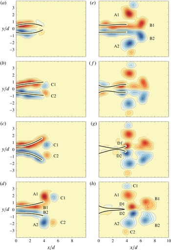
In figure 10, we show the vorticity contours for the sample case of least stiff flaps with
 $L_{f}/d=4$
(same as that in figure 3). At flow initiation in figure 10(a), the flaps bulge outwards in the centre due to an over-pressure, after which the bulge gradually moves outwards resulting in the flap tips opening outwards. In figure 10(b), we can see formation of two vortices (
 $\text{C1}$
and
 $\text{C2}$
) that are due to the outward motion of the flaps, which results in separation of the boundary layer formed on the outer surface of the flaps at the flap tips. In Das et al. (Reference Das, Govardhan and Arakeri2013), we saw similar vortices being formed when the rigid flaps moved outwards. As in that case, we will refer to these vortices as
 $\text{C}$
vortices, which are of opposite sense to the vortices formed if the flaps did not move. As the flaps open out fully and start returning to their initial position, the ensuing fluid starts separating from the flap tips (figure 10
d). These vortices (
 $\text{A}$
) result from the separating boundary layer on the inside surface of the flaps. The
 $\text{A}$
vortices are the ones which would form if the flaps were absent, or if the flaps did not move. Since the flaps open out to sufficiently large angles, there is also flow separation in the flap region due to a diffuser kind of flow, resulting in the formation of
 $\text{B}$
vortices, which can be seen forming in figure 10(d) and that come out of the flaps in figure 10(e). These
 $\text{B}$
vortices are also of the same sense as the
 $\text{A}$
vortices. However, the
 $\text{B}$
vortices not only form due to flow separation in the flap region, but also get a contribution from the flow separation at the flap tips at later times (as seen in figure 10
e). As the piston stops, the flaps collapse inwards (figure 10
f) resulting in the formation of
 $\text{D}$
vortices, which are distinctly visible in figure 10(h). Thus, with the introduction of flexible flaps at the exit, we observe the evolution of four distinct kinds of vortices as opposed to a single vortex pair. The relative strength of these vortices depend on the flap length and the stiffness of the flaps besides
 $U_{p}$
. As discussed in the previous section, all the flaps display qualitatively similar kinematics, hence we expect the formation of all these vortices in all cases, although their individual strengths may vary.
Time sequence of vorticity contours for
 $L_{f}/d=4$
, least stiffness flap case with
 $EI^{\ast }=0.034$
. The piston velocity (
 $U_{p}$
) is
 $18~\text{cm}~\text{s}^{-1}$
, and the piston stops at
 $\unicode[STIX]{x1D70F}\approx 1.3~\text{s}$
corresponding to a final fluid slug length reached of
 $L/d=15$
. In each plot, 20 equally spaced contour levels are shown between (
 $\pm$
)
 $\unicode[STIX]{x1D714}d/U_{p}$
, with the value of
 $\unicode[STIX]{x1D714}d/U_{p}$
being in (a) 1.36, (b) 1.33, (c) 1.35, (d) 1.86, (e) 1.83, (f) 2.38, (g) 2.21, (h) 2.53. The instances shown in the figure are at
 $t/\unicode[STIX]{x1D70F}=$
(a) 0.1, (b) 0.19, (c) 0.28, (d) 0.59, (e) 0.97, (f) 1.03, (g) 1.1, (h) 1.16.

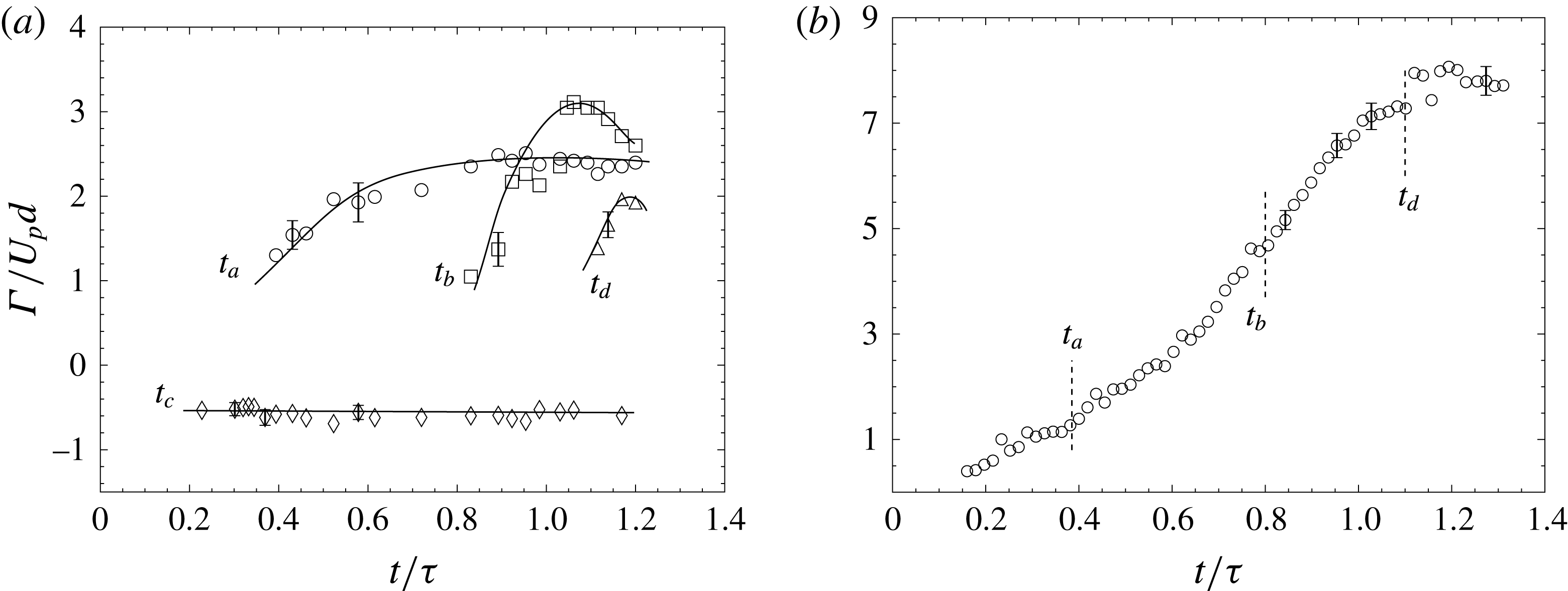
Plot of circulation as a function of time for the sample case shown in figure 10. (a) Circulation of individual vortices as a function of time. (b) The net circulation ejected as a function of time. In both cases, uncertainty in circulation values are shown at representative points.

Figure 11 shows the plot of circulation as a function of time for this sample case. The circulation for each of the individual vortices described before is plotted in figure 11(a) as a function of time. The text
 $t_{a}$
,
 $t_{b}$
,
 $t_{c}$
,
 $t_{d}$
refers to the time at which vortices
 $\text{A}$
,
 $\text{B}$
,
 $\text{C}$
and
 $\text{D}$
are first observed respectively. To compute the value of circulation for, say the
 $\text{A}$
vortices, we measure the circulation of
 $\text{A1}$
and
 $\text{A2}$
separately and then take the average of their absolute values. The uncertainty in the evaluation of circulation obtained from different realizations is also shown on the plot at chosen representative points, indicating that the uncertainties are small compared to the observed variations. The figure shows that the
 $\text{C}$
vortices are formed first at time
 $t_{c}$
and thereafter remain almost constant in strength. The
 $\text{A}$
vortices (at time
 $t_{a}$
) form second and start gaining strength as more and more fluid separates at the flap tips. The
 $\text{A}$
vortices stop growing and the circulation reaches a saturation point when the
 $\text{B}$
vortices form due to separation in the flap region (
 $t_{b}$
). The subsequent vorticity from the boundary layer is then fed to these vortices which start gaining in strength. Once the piston stops at
 $t=1.3~\text{s}$
, fluid from the flap region is pushed out resulting in further growth of these
 $\text{B}$
vortices and making their circulation larger than all other vortices. The rapid closure of the flap tips results in the formation of
 $\text{D}$
vortices at
 $t_{d}$
. The circulations of
 $\text{A}$
,
 $\text{B}$
and
 $\text{D}$
vortices are similar in value whereas the
 $\text{C}$
vortices are the weakest. It should be noted that the relative strengths of these vortices will depend on the kinematics of the flaps for each flap stiffness and length case.
Figure 11(b) plots the total circulation ejected from the flap region. As the fluid gets pushed out of the flap region, the circulation increases continuously with time. Once the piston stops at
 $t/\unicode[STIX]{x1D70F}=1$
, we see that the circulation still keeps increasing because of more fluid being pushed out of the flap region in the form of
 $\text{D}$
vortices (at
 $t_{d}$
). Thereafter, the net circulation reaches a constant final value once the flaps close.
We next look at the fluid impulse of the flow coming out of the nozzle. It has been shown that the impulse (
 $\boldsymbol{I}$
) of a flow given by a velocity field
 $\boldsymbol{u}$
is defined as the time integral of the impulsive force
 $\boldsymbol{F}$
that has to be applied to the flow to generate the velocity field (Saffman Reference Saffman1993; Voropayev & Afanasyev Reference Voropayev and Afanasyev1994; Lighthill Reference Lighthill1996), with
 $\boldsymbol{I}$
being given by:
 $$\begin{eqnarray}\displaystyle & \displaystyle \boldsymbol{I}=\int _{0}^{\unicode[STIX]{x1D70F}}\boldsymbol{F}\,\text{d}t, & \displaystyle\end{eqnarray}$$
where
 $\unicode[STIX]{x1D70F}$
is the time over which the force is applied. This impulse can also be formulated using the vorticity (
 $\unicode[STIX]{x1D74E}$
). This is of interest because the rate of change of fluid impulse is linked to the total non-conservative body forces acting on the fluid. Noca (Reference Noca1997) and Epps (Reference Epps2010) have studied this in detail and provide many expressions for evaluating the time-dependent forces on a body in a fluid, which can be used to estimate the forces on a body from measurements of the flow field around it. DeVoria & Ringuette (Reference DeVoria and Ringuette2013) for example have used this method to evaluate the force on a rotating plate by evaluating the fluid impulse from the measured velocity field. To calculate the fluid impulse in our case, consider a control volume which extends to infinity (
 $V_{\infty }$
) that contains all the fluid which is outside of a control volume
 $V_{b}$
containing the piston cylinder and the flaps. Now, the control volume
 $V_{\infty }$
is large enough to encompass all of the vorticity coming out of
 $V_{b}$
, and the velocity and vorticity become negligible in the limits of its boundaries at
 $x_{\infty }$
and
 $y_{\infty }$
. Since the control volume chosen is such that the volume
 $V_{b}$
(which generates the flow) does not move, we can evaluate the impulse (
 $\boldsymbol{I}$
) of the fluid contained in
 $V_{\infty }$
using the expression:
 $$\begin{eqnarray}\displaystyle & \displaystyle \boldsymbol{I}=\unicode[STIX]{x1D70C}\int _{V_{\infty }}(\boldsymbol{x}\times \unicode[STIX]{x1D74E})\,\text{d}{\mathcal{V}}. & \displaystyle\end{eqnarray}$$
We are interested in the impulse in the
 $x$
direction since the impulse in the
 $y$
direction will be zero because of flow symmetry about the
 $x$
axis. For a two-dimensional flow field, equation (4.2) simplifies to
 $$\begin{eqnarray}\displaystyle & \displaystyle I_{x}=\unicode[STIX]{x1D70C}\int _{A}y\,\unicode[STIX]{x1D714}_{z}\,\text{d}A, & \displaystyle\end{eqnarray}$$
where
 $A$
is a large enough area which includes all the vorticity and
 $I_{x}$
is evaluated per unit depth.
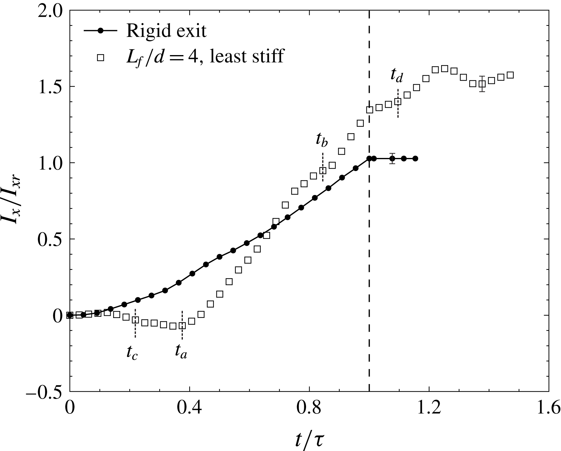
Plot of impulse as a function of time for the sample case shown in figure 10 along with a rigid exit case. All the other parameters for the two cases are the same. The times
 $t_{a}$
,
 $t_{b}$
,
 $t_{c}$
,
 $t_{d}$
at which the vortices
 $\text{A},~\text{B},~\text{C}$
and
 $\text{D}$
are first observed respectively are also marked in the plot for the flap case. Uncertainty in impulse values are shown at representative points for both cases. The piston stops at the dotted line along the
 $x$
axis when the fluid slug length
 $(L/d)$
reached is 15.

From our experimental data, this impulse is evaluated by taking a large flow field which encompasses all the vorticity that has come out of the flap region. We do this by masking the flaps along with the region contained between the flaps and then processing the images to get the flow field. A large enough field of view ensured that all the vorticity was contained within the control volume and that the fluid velocities were sufficiently small on the outer boundaries for the duration studied. The
 $x$
component (streamwise) of the impulse is plotted in figure 12 for the rigid exit case and for the sample flap case. Although not shown here, the
 $y$
component is approximately zero because of flow symmetry. We notice that by introducing the flaps at the exit of the channel, the fluid impulse changes dramatically in comparison to the rigid exit case, where the impulse increases almost linearly until the piston stops (similar to figures 18 and 19 in Krieg & Mohseni (Reference Krieg and Mohseni2013)). In the rigid case, after the piston stops, the impulse of the flow becomes nearly a constant value (
 $I_{xr}$
).
In the flaps case, the times
 $t_{a}$
,
 $t_{b}$
,
 $t_{c}$
,
 $t_{d}$
at which the vortices
 $\text{A},~\text{B},~\text{C}$
and
 $\text{D}$
are, respectively, first observed, are also marked in the plot. Initially, as the flaps bulge, the impulse is close to zero as all the vorticity is present only within the flap region. As the flap tip opens outwards, the
 $\text{C}$
vortices that are of opposite sign to the other vortices start to form at time
 $t_{c}$
outside the flap region, and we find that the impulse of the fluid becomes negative due to the opposite sign of
 $\text{C}$
vortices. Subsequently as the flaps close, the
 $\text{A}$
vortices begin to form at
 $t_{a}$
with their strengths being much larger and of opposite sign to the
 $\text{C}$
vortices. This leads to a very rapid increase in the impulse, with the rate of increase of impulse being considerably larger than the rigid exit case. The increase in impulse continues at approximately the same rate as
 $\text{B}$
vortices are formed and add to the total impulse. The impulse data in the flap case are approximately linear between
 $t/\unicode[STIX]{x1D70F}\approx 0.4$
and 1, with a slope of approximately 1.8 times that of the slope of the impulse data for the rigid exit case. This indicates that the net force is significantly higher for the flap case over a reasonable amount of time. Once the piston stops, unlike in the rigid exit case, the impulse of the fluid continues to increase, but at a slower rate than before. This is due to the fact that after the piston stops, the flaps close rapidly but over some finite time, during which they continue to push out more fluid and vorticity resulting in a larger total impulse in the end. The final impulse of the sample flap case shown is approximately 60 % higher compared to the final impulse of the rigid case (
 $I_{xr}$
).
The final impulse can also be understood as the product of the final circulation (
 $\unicode[STIX]{x1D6E4}=\int \,\unicode[STIX]{x1D714}_{z}\,\text{d}A$
) and an effective lateral spacing (
 $y_{eff}$
) between the two oppositely signed regions of vorticity. We can therefore determine
 $y_{eff}$
from (4.3) as:
 $$\begin{eqnarray}\displaystyle & y_{eff}={\displaystyle \frac{\displaystyle \int y\,\unicode[STIX]{x1D714}_{z}\,\text{d}A}{\unicode[STIX]{x1D6E4}}}. & \displaystyle\end{eqnarray}$$
This effective lateral separation distance can be thought of as the distance between the centroid of the vorticity on each side of the line of symmetry (
 $x$
axis). Knowing the final fluid impulse and the final circulation, we can then find the corresponding
 $y_{eff}$
. Therefore, for the same circulation, a higher impulse would imply a higher
 $y_{eff}$
. The results thus suggest that in the flap case, the opening of the flaps results in larger
 $y_{eff}$
due to vorticity redistribution, thereby increasing the final fluid impulse. We shall see in the following subsections that this is broadly true for all the flap cases, with the final impulse and
 $y_{eff}$
being larger for nearly all the flap cases compared to the rigid exit case.
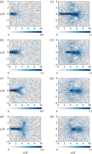
Instantaneous streamlines along with velocity magnitude contours for the sample case with least flap stiffness and
 $L_{f}/d=4$
. The colour variation shows the absolute velocity magnitude of the fluid normalized with the piston speed. All the parameters are the same as in figure 10.

We next plot the streamlines for the sample case in figure 13 along with colour contours of the fluid velocity magnitude. This combination of streamlines and velocity magnitude normalized by the piston speed gives a broad overview of the fluid motion in the vicinity of the flaps at different times. Due to the initial bulge (figure 13
a), the ambient fluid is displaced creating a flow resembling potential flow outside the flap region. As the flaps open outwards, the streamlines close to the flaps follow the flap deformation profile. Until the instance shown in figure 13(c), the fluid velocity outside of the flap region is very small suggesting that most of the fluid has until now only been accommodated in the extra volume created by the flaps opening out. At instance (d), the rolling up of the streamlines shows the formation of
 $\text{A}$
vortices at the flap tips. At instance (e), we see large fluid velocities outside of the flap region and in between the vortices that are due to two reasons. The first reason is that the flaps moving inwards pushed fluid out of the flap region adding to the fluid being pushed by the piston, resulting in larger fluid velocities. The second reason is the induced flow created by the vortices on either side of this jet of fluid. At the instance seen in figure 13(f), the collapsing flaps result in the fluid being dragged in to fill the space created on the outer side of the flaps. Once the flaps begin to close the fluid starts getting pushed out of the flap region. This results in large fluid velocities in between the vortices as seen in figure 13(g). In instance (h) the flaps have closed fully and we see that the fluid velocity in some regions has reached almost 1.35 times the piston speed (
 $U_{p}$
). The streamlines here show that the fluid velocities are large and concentrated in the region between the vortices.
4.2 Effect of flap stiffness and length on vortex dynamics
We shall now present time sequences of the flow field for variations in flap stiffness and flap length along with the corresponding circulation and impulse values. Figure 14 shows the vorticity contours for three different flap stiffness cases (
 $EI^{\ast }$
), all with
 $L_{f}/d=6$
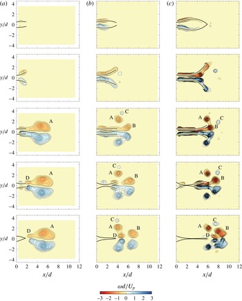
. The instances shown in each case, as before, are at the maximum bulge, at the maximum opening, just before piston stops, after piston stops and after all the fluid has been ejected out. The contour levels which are plotted are kept the same for all the cases. It is clear that although the flow fields are qualitatively similar, there are important differences as well. For example, distinct
 $\text{B}$
vortices are formed in the least stiff case in figure 14(a), while in the stiffest case in figure 14(c), the
 $\text{B}$
vortices can hardly be seen. This difference may be attributed to the flaps considerable opening out in figure 14(a), which leads to flow separation within the flap region that leads to formation of
 $\text{B}$
vortices, while the flaps do not open out as much in the stiffer case in figure 14(c), preventing flow separation. In addition to the larger opening in figure 14(a), it should also be noted that the least stiff flaps also open more gradually giving larger times for the flow to separate as compared to the stiff flap cases. Differences can also be seen with respect to the formation of
 $\text{C}$
vortices formed during the outward motion of the flap tips. These
 $\text{C}$
vortices can be seen clearly in figure 14(a) and (b). In the stiffest flap case in figure 14(c), the initial bulge and subsequent opening of the flap tips happens very rapidly, resulting in a to and fro motion of the flap tips. This results in the formation of a vortex pair near each flap tip seen in the second image (of figure 14
c), which then quickly shoot out in the transverse direction, thus removing the
 $\text{C}$
vortices from the flap tip region. These differences lead to significant changes in the final vorticity configuration in the three cases indicating that the stiffness of the flaps is an important parameter in determining the flow.
Plot showing time sequence of vorticity contours for (a) least stiff flaps,
 $EI^{\ast }=0.028$
(b) intermediate stiffness flaps,
 $EI^{\ast }=0.096$
and (c) stiffest flaps,
 $EI^{\ast }=0.49$
. The flap length is
 $L_{f}/d=6$
and the increment between successive vorticity (
 $\unicode[STIX]{x1D714}d/U_{p}$
) contour levels is approximately 0.14 in each case. The piston speed
 $U_{p}\approx 18~\text{cm}~\text{s}^{-1}$
, and the piston stops when the fluid slug length reached is
 $L/d=15$
. The different times for each flap stiffness are the time taken for maximum bulge, maximum opening, the time just before piston stops, just after piston stops and the time taken for complete closure of the flaps respectively from top to bottom of the plot. The instantaneous time (
 $t/\unicode[STIX]{x1D70F}$
) for each instance is shown in the figure.

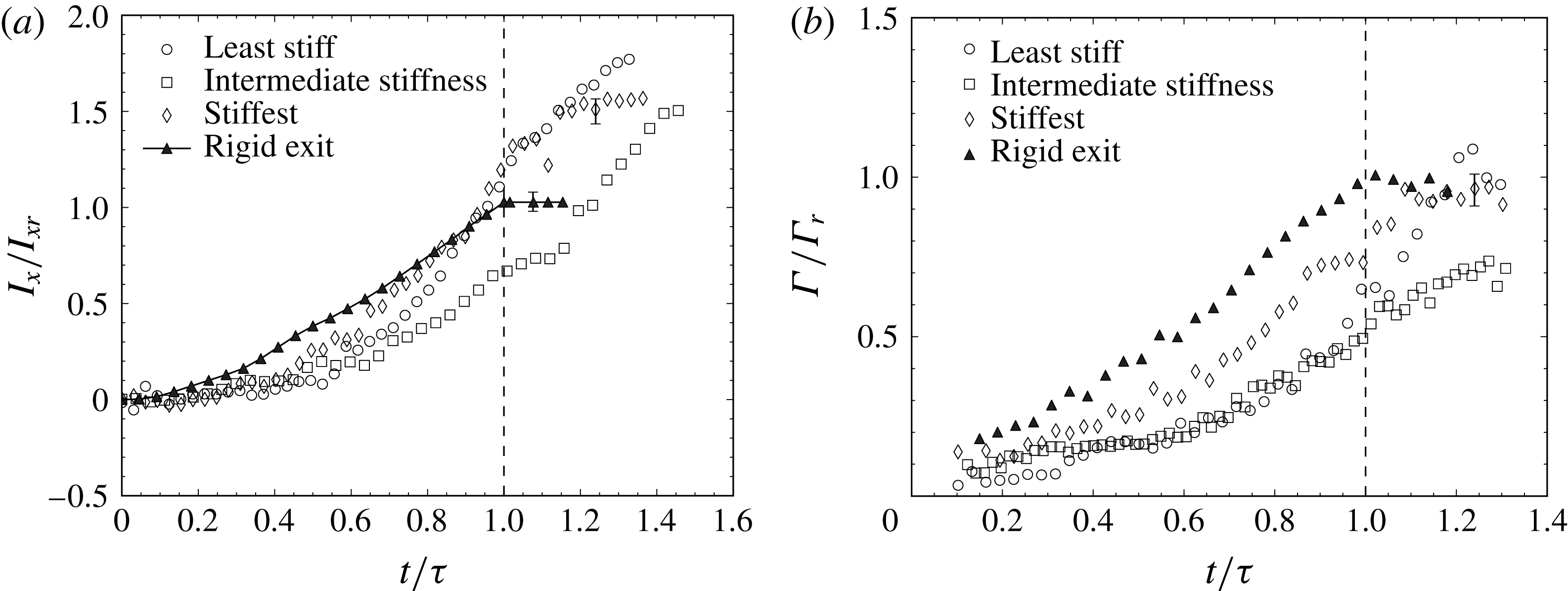
Plot of (a) impulse as a function of time and (b) circulation as a function of time, for different flap stiffness cases along with the rigid exit data. Uncertainty estimates are shown at a few representative points. In all cases, the flap length (
 $L_{f}/d$
) is 6, the piston speed
 $U_{p}\approx 18~\text{cm}~\text{s}^{-1}$
, and the final fluid slug length
 $(L/d)$
reached is 15. The piston stops at the dotted line along the
 $x$
axis, where the fluid slug length
 $(L/d)$
is 15.

In figure 15, we plot the impulse (figure 15
a) and the circulation (figure 15
b) for the three flap stiffness cases discussed above along with the reference rigid exit case. Both the impulse (
 $I_{x}$
) and circulation (
 $\unicode[STIX]{x1D6E4}$
) values are normalized by the final impulse (
 $I_{xr}$
) and circulation (
 $\unicode[STIX]{x1D6E4}_{r}$
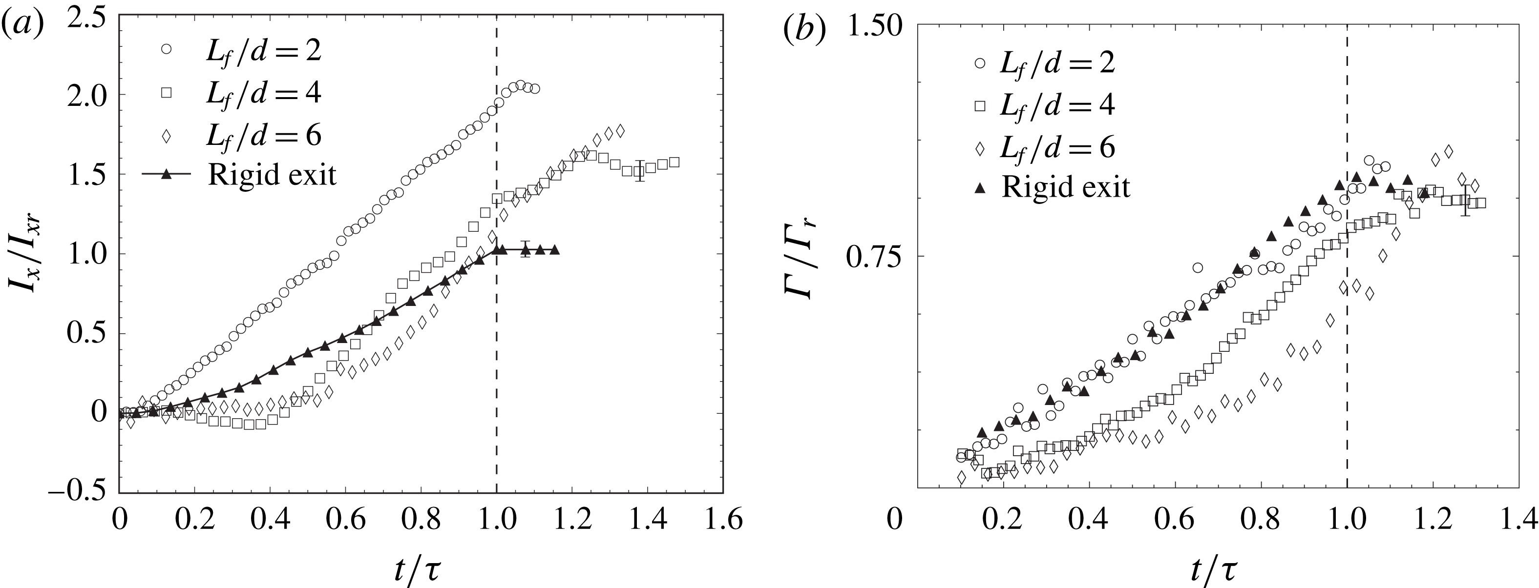
) values of the rigid exit case. With respect to the impulse, the most important point to note is that the final impulse of the flow is higher in all the flap cases when compared to the rigid exit case, with the final impulse being about 1.5 to 1.75 times higher than the rigid exit case. In all three cases, we can see that there are some common characteristics of the impulse variation with time, while there are also some distinct differences. In all flap cases, the impulse does not immediately increase after the flow starts due to the bulging of the flaps, which leads to very little vorticity ejection from the flap region. Subsequently, the impulse increases in all cases with the rise being more rapid in the least and stiffest cases, compared to the intermediate stiffness case, although the final impulse values are all reasonably similar. The differences with stiffness may be better understood by simultaneously looking at the circulation values for the three cases. In the stiffest flap case, the flaps do not open out as much and hence vorticity is ejected from the flap region relatively early and therefore shows up as an earlier rise in circulation in the plot compared to the intermediate and least stiff flaps. In these latter two cases, the flaps open out more, and hence the vorticity takes longer to be ejected from the flap region, and hence the circulation rise is delayed. We find that the final circulation values reached are similar for the most and least stiff flap cases both of which are also close to the rigid exit case. This suggests that in these cases, the net circulation is about the same but is redistributed to have a higher impulse, which is linked to the larger lateral separation (
 $y_{eff}$
) between the two opposite regions of vorticity as discussed in the previous subsection. In the intermediate stiffness case, we find that the final circulation values are a little lower (approximately 15 %), which is likely linked to cancellation of opposite signed vorticity within the flap region. The reason for the larger vorticity cancellation in this intermediate stiffness case may be related to the larger time taken for opposite signed vorticity within the flap region to be ejected in this case, compared to both the least and most stiff flap cases. This can be seen in figure 14 and especially figure 15(b), where the intermediate and least stiff flap cases have nearly the same circulation ejected until the instant when the piston stops (
 $t/\unicode[STIX]{x1D70F}=1$
). Thereafter, in the least stiff flap case, the circulation rapidly increases as the flaps swiftly deform and eject vorticity, while in the intermediate stiffness case, a much more gradual increase in circulation is seen related to the slower ejection of vorticity. In contrast to these, the stiffest flap has a circulation variation with time that is much more rapid right from the start of piston motion and closer to that of the rigid case, as the flaps do not deflect as much as the least or intermediate stiffness cases. Related to this, one can also notice a more diffuse vorticity field in the intermediate stiffness case. In general, more diffuse vortices are seen to form when the motions of the flap as a whole are more gradual, and the flap has no rapid local deformations near the flap tip. On the other hand, more tightly rolled up vortices are seen to form when there are rapid local deformations near the flap tip (least stiff flap case) and when the flap as a whole has more rapid motions (stiffest flap case).
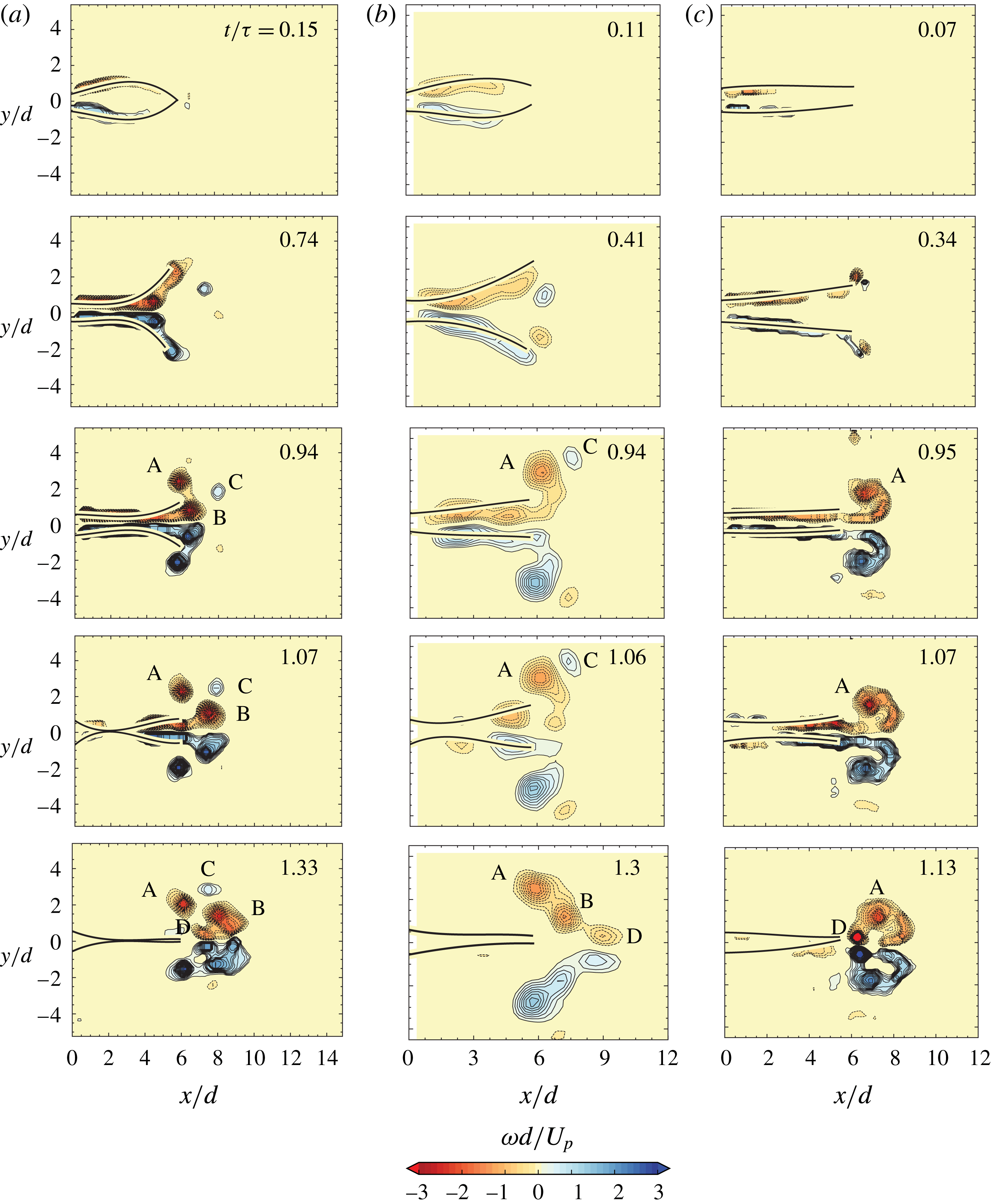
Plot showing time sequence of vorticity contours for (a)
 $L_{f}/d=2$
, (b)
 $L_{f}/d=4$
and (c)
 $L_{f}/d=6$
. The flap stiffness (
 $EI$
) is the least in each case, and the piston speed
 $U_{p}\approx 18~\text{cm}~\text{s}^{-1}$
, thus giving
 $EI^{\ast }$
values of 0.097, 0.035 and 0.028, respectively, in the three cases. The different times for each flap length case shown are the time taken for maximum bulge, maximum opening, the time just before piston stops, just after piston stops and the time taken for complete closure of the flaps respectively from top to bottom. The time instances are the same as shown in figure 7 and the increment between successive vorticity contour levels is approximately 0.14 in each case.

We now look at the effect of flap length
 $L_{f}/d$
while keeping the flap material and hence the flap stiffness (
 $EI$
) constant. Figure 16 shows the vorticity contours for the least stiff flap case (
 $EI=2\times 10^{-5}~\text{Nm}$
). We choose this flap stiffness because it undergoes larger deformations and therefore shows more pronounced differences in flow features. The flap lengths used are
 $L_{f}/d=2$
(figure 16
a),
 $L_{f}/d=4$
(figure 16
b) and
 $L_{f}/d=6$
(figure 16
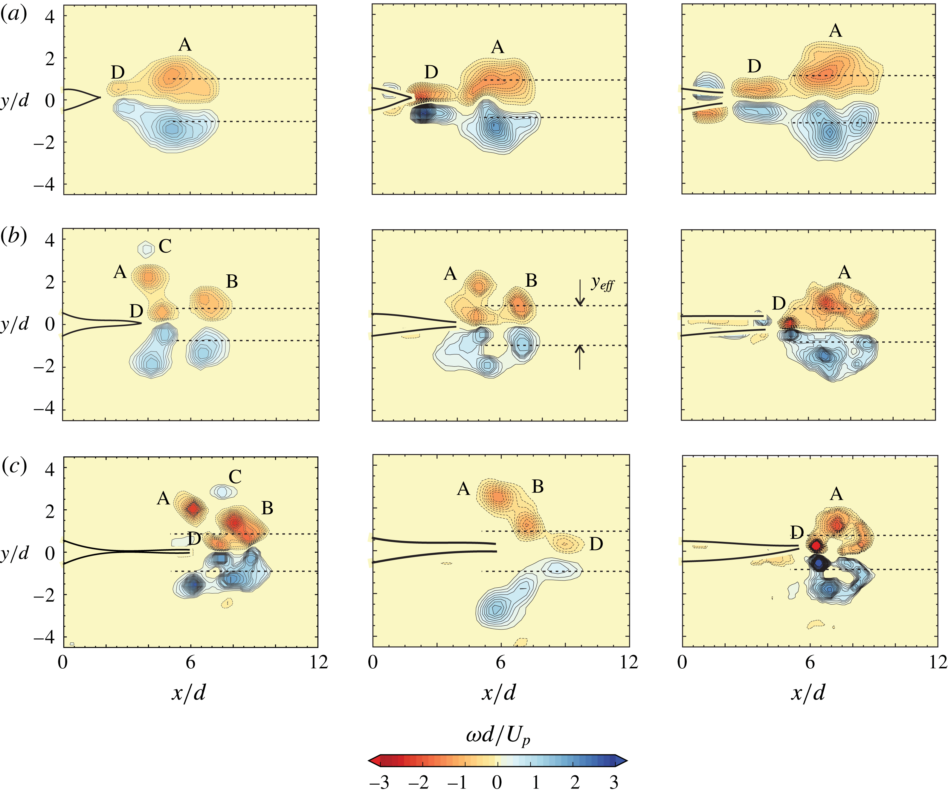
c). The instances shown are the same as in figure 7 with the vorticity contour levels shown being the same in all cases. It is clear that there are important changes in the vorticity dynamics as the flap length is varied. For the longest flap case (
 $L_{f}/d=6$
), when the flaps are at their maximum opening, there is a very clear flow separation in the flap region due to the large angle created by the flaps. This results in the formation of
 $\text{B}$
vortices and these can be clearly seen at this instance. In contrast, the
 $\text{B}$
vortices are not as strong in the
 $L_{f}/d=4$
case, and are completely absent in the
 $L_{f}/d=2$
case, where the flap opening is relatively small. In this latter case (
 $L_{f}/d=2$
), both the
 $\text{B}$
and
 $\text{C}$
vortices cannot be seen and only strong
 $\text{A}$
vortices and relatively weaker
 $\text{D}$
vortices corresponding to flap closing can be seen. In the
 $L_{f}/d=4$
and
 $L_{f}/d=6$
cases, we can see all the different types of vortices
 $\text{A}$
,
 $\text{B}$
,
 $\text{C}$
and
 $\text{D}$
, although their relative strengths are different. The final vorticity configuration in the three cases shows significant differences, as seen in the final image of each sequence, highlighting the importance of flap length on the flow.
(a) Impulse as a function of time and (b) circulation as a function of time, for different flap length cases along with the rigid exit data. In all cases, the flap stiffness (
 $EI$
) is the least, the piston speed
 $U_{p}\approx 18~\text{cm}~\text{s}^{-1}$
and the final fluid slug length
 $(L/d)$
reached is 15. The piston stops at the dotted line along the
 $x$
axis, where the fluid slug length
 $(L/d)$
is 15.

Plot of the normalized volume flow rate out of the flap region as a function of time for (a) the
 $L_{f}/d=6$
case with variations in flap stiffness, and (b) for the least stiff (
 $EI$
) flap case with variations in flap length. The filled symbols in each case show the time instance when the maximum flap tip opening occurs. The rigid exit case is shown by the solid line in both plots. In each case, the piston velocity
 $U_{p}\approx 18~\text{cm}~\text{s}^{-1}$
, and the final fluid slug length
 $(L/d)$
reached is 15.

The impulse and circulation values as a function of time for the three different flap length cases are shown in figure 17(a) and (b), respectively. As before, the final impulse is higher in all the flap cases compared to the rigid exit case with the largest value being for the shortest flap (
 $L_{f}/d=2$
) case that has a final impulse that is approximately twice the value of the rigid exit case. Among the different flap length cases, the
 $L_{f}/d=2$
case is strikingly different. One can see a clear rise in impulse within a relatively small time after flow initiation, as circulation is relatively rapidly ejected from the flap region for this short flap case, as shown in figure 17(b). The impulse increases approximately linearly until slightly after the piston stops, with the slope of this line being roughly twice that of the rigid exit case. We will see later in § 4.3 that this is related to the overall configuration of vorticity, more precisely to the extent of lateral motion of the centroid of vorticity that we shall see is the largest for this case. Compared to the
 $L_{f}/d=2$
case, the longer flaps take larger times after flow initiation before they show a significant rise in impulse as the vorticity takes longer to emerge from the flap region, consistent with the measurement of circulation shown in figure 17(b). The time taken for the circulation to rise from around zero is longest for the
 $L_{f}/d=6$
case, as might be expected, with the final circulation however being nearly the same in all three cases and equal to the rigid case, as observed before. It may be noted here that the non-dimensional flexural rigidity or stiffness (
 $EI^{\ast }$
) value for the
 $L_{f}/d=2$
case (figure 16
a) is approximately 0.097, which is nearly the same as the intermediate stiffness case (with
 $L_{f}/d=6$
) shown in figure 14(b). Clearly, although the two have nearly the same values of
 $EI^{\ast }$
, the vorticity distribution and the time variation of the impulses are very different indicating that
 $EI^{\ast }$
alone is not sufficient to determine the vorticity dynamics, although it does give a reasonable collapse of the flap kinematics as shown in the previous section.
We shall now highlight the effect that flap deformation has on the net volume flow rate out of the flexible flap exit (
 $\dot{Q}$
). The volume flow rate out of the rigid exit is completely determined in our incompressible case by the piston speed (
 $U_{p}$
), as is shown by the solid line in figure 18, which is representative of the near impulsive piston velocity program used in our study. We define
 $\dot{Q}_{r}$
as the flow rate associated with the constant speed portion of this velocity program for the rigid exit case, and use this to normalize the flow rate for all the flap cases shown in the figure, with effects of variations in
 $EI$
of the flap being shown in figure 18(a) and effects of variations in flap length (
 $L_{f}/d$
) shown in figure 18(b). In the flexible flap cases, the flap deformations change with time, leading to the possibility of transient storage and expulsion of fluid within the flap region, and hence, the flow rate out of the flap region can vary significantly from the piston velocity program. In these cases, we have another term that is dependent on the rate of change of volume contained within the two (deforming) flaps, which we evaluate from the recorded flap deformation profiles at different instances in time. Initially, as the flaps bulge out, the volume flow rate out of the flexible exit is less as the flow pushed out by the piston is taken up to fill the increasing volume between the two flaps, with this effect being more pronounced for the longer and lower stiffness cases. Subsequently, as the region between the flaps stops expanding, the flow rate out (
 $\dot{Q}$
) equals
 $\dot{Q}_{r}$
that is pushed by the piston. It may be noted that the time instance where the maximum flap tip opening occurs, shown by the filled symbols in the plot, does not correspond to
 $\dot{Q}$
equals
 $\dot{Q}_{r}$
, as the latter condition corresponds to the case where the volume of the region between the flaps is maximum. As the volume of the region between the flaps begins to reduce, the fluid between the flaps is pushed out in addition to the fluid pushed out by the piston leading to substantially higher volume flux than
 $\dot{Q}_{r}$
, reaching values of approximately
 $2\dot{Q}_{r}$
. One can also see that the volume flux out continues to be non-zero even after the piston stops, this being caused by the collapsing flaps that continue to push fluid out from the flap region. These effects can be seen in all the different flap stiffness and length cases shown in figure 18, although the extent of these effects vary, with the more pronounced effects being seen for the less stiff (in figure 18
a) and the longer flap cases (in figure 18
b). In the smallest flap case (
 $L_{f}/d=2$
) in figure 18(b), the changes in volume between the flaps is relatively small, and the volume flow rate is reasonably close to the flow rate generated by the piston motion alone, except during the initial times and after the piston stops.
4.3 Final vorticity configuration
We now present in figure 19 the final vorticity configuration, after all of the fluid has left the flap region, for the different flap stiffness (
 $EI$
) and flap length (
 $L_{f}/d$
) cases studied. The time at which this occurs is different for each case, but it gives an overall picture of the final flow configuration. In the figure, the flap length increases as we go from top to bottom, and the stiffness increases as we go from left to right. In each case, the different kinds of vortices (
 $\text{A}$
,
 $\text{B}$
,
 $\text{C}$
and
 $\text{D}$
) are labelled and one can see the significant changes with stiffness and flap length. For the shortest flap length of
 $L_{f}/d=2$
, only the
 $\text{A}$
and
 $\text{D}$
vortices are present. This is because the time in which the flaps open and return to their initial position is small and therefore the flow does not separate in the flap region to form the
 $\text{B}$
vortices. In the other two flap length cases, all these vortices are present. The stiffest flaps however, irrespective of the flap length, do not clearly show the formation of
 $\text{B}$
and
 $\text{C}$
vortices. The
 $\text{D}$
vortices in all the
 $L_{f}/d=4$
and
 $L_{f}/d=6$
cases move reasonably fast compared to the other vortices and often either merge with the
 $\text{B}$
(and/or
 $\text{A}$
) vortices or overtake them (as in the
 $L_{f}/d=6$
, intermediate stiffness case). This can be attributed to the fact that the
 $\text{D}$
vortices are generated by a rapid inward motion of the flaps after the piston stops. This results in the formation of vortices which are laterally less spread out compared to the
 $\text{A}$
,
 $\text{B}$
and
 $\text{C}$
vortices. This would mean that the self-induced velocity of this pair would be higher as observed in the experiments. The final configuration of the vorticity out of the flap region is thus dramatically different with the introduction of flexible flaps and varies with the flexural rigidity and length of the flaps. However, in almost all the cases, the total circulation ejected from the flap region is nearly the same as the rigid exit case, indicating that the total circulation is shared among the different vortices seen in each case.
Vorticity contours for the flap cases at the instance when all the fluid has been ejected from the flap region after the piston stops. The flap length increases from
 $L_{f}/d=2$
to
 $L_{f}/d=6$
from the top to bottom image, and the stiffness (
 $EI$
) increases from least to most as we go from left to right. The
 $EI^{\ast }$
values for (a) (
 $L_{f}/d=2$
) from left to right are 0.097, 0.69, 3.84 respectively; for (b) (
 $L_{f}/d=4$
) from left to right are 0.035, 0.18, 1.01 respectively; for (c) (
 $L_{f}/d=6$
) from left to right are 0.028, 0.096, 0.49 respectively. In all cases, the piston speed
 $U_{p}$
is
 $18~\text{cm}~\text{s}^{-1}$
, and the piston stops when the fluid slug length reached is 15. The increment between successive vorticity contour levels is approximately 0.14 in each case.

The final vorticity contours for (a) rigid exit case, (b) hinged-rigid flap cases (
 $L_{f}/d=2$
& 4), (c) least stiff flexible flap cases (
 $L_{f}/d=2$
& 4). The instance chosen is when all the fluid has been ejected after the piston stops. The piston velocity program is impulsively started in each case with the piston speed being
 $18~\text{cm}~\text{s}^{-1}$
in the rigid and flexible flap cases, and
 $5.5~\text{cm}~\text{s}^{-1}$
for the hinged-rigid flap cases (Das et al.
Reference Das, Govardhan and Arakeri2013), with the final fluid slug reached in all cases being close to 15. The increment between successive vorticity contour levels is approximately 0.14 in each case.

The present study has been done with deformable flexible flaps having a flexural rigidity or stiffness (
 $EI$
). In a previous study, Das et al. (Reference Das, Govardhan and Arakeri2013) studied the case of hinged-rigid flaps with negligible hinge stiffness, and a comparison of the final vorticity configurations between the two studies is shown in figure 20 along with the reference rigid exit case. Since the study of Das et al. (Reference Das, Govardhan and Arakeri2013) was for the negligibly small hinge stiffness case, we choose for the comparison, low stiffness cases from our present study, and in particular show two flap length cases
 $L_{f}/d=2$
and
 $L_{f}/d=4$
. The first observation is that qualitatively the vorticity field is very different from the rigid exit case for all flap cases. Comparing the hinged-rigid flaps and the deformable flap cases, we can see that there are some striking similarities and some distinct differences. There is a clear similarity across both flap types for the
 $L_{f}/d=2$
and
 $L_{f}/d=4$
cases, with the shorter flap showing just a relatively simple configuration in both cases, while the longer flap cases have a more complex distribution of vorticity with the formation of many different types of vortices. A distinct difference between the two flap types is the clear formation of separate vortices
 $\text{A}$
,
 $\text{B}$
,
 $\text{C}$
and
 $\text{D}$
in the deformable flap case with
 $L_{f}/d=4$
, in contrast to the hinged-rigid case where the different vortices are present, but are not as clear. The same is true for the
 $L_{f}/d=2$
case, where the
 $\text{D}$
vortices are somewhat clearer in the deformable flap case as compared to the hinged-rigid flap case. These differences appear to be linked to the fact that in the flexible flap cases, the deformations can be local and rapid (say near the flap tips) and hence permits clear formation of distinct vortices, while in the hinged-rigid flap case, the entire flap would respond more slowly as it has to move as a whole in response to the fluid forces.
Figure showing the plot of final (a) impulse (b) circulation and (c)
 $y_{eff}$
for all the flap cases as a function of
 $EI^{\ast }$
. The impulse and circulation values are normalized by the corresponding rigid exit case values. Symbols are: ○,
 $L_{f}/d=2$
; ▫,
 $L_{f}/d=4$
; ♢,
 $L_{f}/d=6$
; with open symbols for least stiff, half-filled for intermediate and filled for stiffest flaps. The open symbols with a dot inside are for the corresponding hinged leaflet cases from Das et al. (Reference Das, Govardhan and Arakeri2013). In (a) and (b) the values are normalized by the corresponding rigid exit case. In (c), for reference,
 $y_{eff}/d\approx 1$
for the rigid exit case.

Figure 21 shows final fluid impulse (figure 21
a), final circulation (figure 21
b) and
 $y_{eff}/d$
(figure 21
c) for all the flap cases plotted against the non-dimensionalized flexural rigidity (
 $EI^{\ast }$
). In addition to the present data, the hinged-rigid data from Das et al. (Reference Das, Govardhan and Arakeri2013) corresponding to nearly zero stiffness are also shown in each plot of the figure. The impulse and circulation values have been normalized with the corresponding rigid exit values, with both plots showing that the data are relatively insensitive to
 $EI^{\ast }$
over the range of
 $EI^{\ast }$
values studied from nearly zero to approximately 10, although there is some variation. The uncertainties in both impulse and circulation are shown by uncertainty bars for all the cases in figure 21. While these experimental uncertainties are present, the impulse values are still significantly higher compared to the rigid exit values whereas the net ejected circulation values are close to the rigid exit value. For the impulse values, the variations across different stiffness cases also appears to be real and not because of measurement uncertainties. As noted before, the flap deformations in these different cases can vary significantly (as shown in § 3), and
 $EI^{\ast }$
only broadly collapses the maximum flap tip opening data. This implies that considerable differences in vorticity distribution can result from the variations in flap deformation, even for the same
 $EI^{\ast }$
, as highlighted by the differences in vorticity distribution between figures 14(b) and 16(a) (both having the same
 $EI^{\ast }$
). Hence, variations, such as those seen in figure 21, between the different flexible flap cases are not surprising, although it is not easy to explain them. Despite these complexities, a broad overall result is that the final fluid impulse in the cases with flaps (
 $I_{x}$
) is approximately twice the impulse values in the rigid exit case (
 $I_{xr}$
), as shown by the dashed line in figure 21(a) over the range of
 $EI^{\ast }$
values studied.
As
 $EI^{\ast }$
increases, we expect the normalized impulse to reduce gradually to the rigid exit value of 1.0. The circulation plot shows that the final circulation in all cases is about the same as the rigid exit case, although there are some variations. The increase in impulse is thus mainly related to the changes in the lateral spacing of the generated vortices (
 $y_{eff}/d$
). This is reflected in the
 $y_{eff}/d$
plot, which is qualitatively similar to the impulse plot, with
 $y_{eff}/d$
being approximately about 2 over the range of
 $EI^{\ast }$
values studied. We mark this distance in figure 19 by drawing two dotted lines in each vorticity plot, the distance between them being
 $y_{eff}/d$
. At higher
 $EI^{\ast }$
values,
 $y_{eff}/d$
is expected to reduce gradually to the rigid case value of approximately 1.0 as
 $EI^{\ast }$
tends to large values. It may also be seen that the data for the hinged-rigid flap cases (Das et al.
Reference Das, Govardhan and Arakeri2013), with nearly zero stiffness, are broadly in agreement with the present deformable flap cases in each of the three plots. Overall the motion of the flaps, as discussed in detail before, leads to a redistribution of vorticity, which in turn results in higher final impulse values.
In this section, we have looked at the effect of flap stiffness (
 $EI$
) and flap length (
 $L_{f}/d$
) on the vorticity dynamics. The results show that even when the non-dimensional flexural rigidity (
 $EI^{\ast }$
) is maintained (as in figures 14(b) and 16
a), the detailed vorticity dynamics varies with flap length (
 $L_{f}/d$
). This indicates that
 $EI^{\ast }$
alone is not sufficient to determine the detailed vorticity dynamics, although it does give a reasonable collapse of the flap kinematics and integrated quantities such as the total final impulse. The observed differences for example in the final normalized impulse about the mean value of 2 appear to be related to these observed differences in the vorticity dynamics. In general, the formation of up to four kinds of vortices were observed with the introduction of flaps at the exit, which we refer to as
 $\text{A}$
,
 $\text{B}$
,
 $\text{C}$
and
 $\text{D}$
, along with significant changes in the final impulse of the flow that can be more than 100 % higher than the rigid exit case. The rate at which impulse increases, which is linked to force, was also found to be substantially higher over a significant time for the flexible cases in comparison to the rigid exit case.
5 Conclusions
We experimentally study the effect of exit flexibility on the formation of a two-dimensional starting jet that is frequently observed in many biological systems as in the propulsive action of squids and in the human heart. These biological systems are made of flexible membranes/tissues which makes it pertinent to study the effect of flexibility in such flows, although the configuration and parameters chosen for the present work do not represent any particular biological system. The chosen configuration can be thought of as a model/simplified problem for understanding the effects of flexibility on flow generation for the relatively more complex biological systems, besides being of interest for the development of efficient pulsed jet based propulsion systems. This is an extension of our previous study on passively hinged-rigid flaps at the nozzle exit (Das et al.
Reference Das, Govardhan and Arakeri2013) by introducing flexibility in the form of deformable flaps that have an inherent flexural rigidity (
 $EI$
). The flexural rigidity (
 $EI$
) thus becomes an important parameter in the problem, along with the flap length (
 $L_{f}/d$
) and the piston velocity program (
 $d=$
channel width). We have studied three different flap stiffness values (
 $EI$
), flap lengths (
 $L_{f}/d=2$
, 4 & 6) and a range of impulsively started piston velocity programs defined by the constant piston speed (
 $U_{p}$
). In all cases, the flexible flaps are attached at the exit of a large aspect ratio channel with the flaps initially being parallel to the channel walls. The flow is set-up by pushing a piston through the channel with an impulsively started piston velocity profile defined by the piston speed (
 $U_{p}$
) that was varied from 10 to
 $25~\text{cm}~\text{s}^{-1}$
.
The flap kinematics in all cases are qualitatively similar. As the piston starts we first notice that the flaps bulge near the channel exit. This is due to the excess pressure (Krueger Reference Krueger2005; Das et al.
Reference Das, Govardhan and Arakeri2013) created in the flap region because of the acceleration that has to be imparted to the fluid slug between the flaps. This bulge then increases in size as well as moves downstream resulting in the eventual opening out of the flaps. After the flap tips separate out and reach a maximum opening, the flaps start returning to their initial position. The flaps remain in this parallel configuration until the piston stops. Once the piston stops impulsively, the flaps collapse inwards near the channel exit, caused by the low pressure due to sudden deceleration (Lee & Talbot Reference Lee and Talbot1979). The flap closure causes additional fluid from the flap region to be pushed out compared to the rigid exit case. We find that the flap’s flexural rigidity (
 $EI$
) played an important role in its kinematics. We define a non-dimensional flexural rigidity
 $EI^{\ast }$
to look at the effect of
 $EI$
. We find that across different values of flap stiffness and length, and varying piston speeds, the maximum opening angle of the flaps decreases linearly with increasing values of log(
 $EI^{\ast }$
). The time taken by the flaps to reach the maximum opening (
 $L/L_{f}$
) also approximately falls on a single curve for all the cases studied, when plotted with
 $EI^{\ast }$
.
Flap shapes for all the flap cases at (a) the instance when the flaps have reached their maximum initial bulge, and (b) when the flap tips have reached their maximum opening. Piston velocity program is impulsively started in each case with the piston speed being
 $18~\text{cm}~\text{s}^{-1}$
. Piston stops at
 $\unicode[STIX]{x1D70F}=1.3~\text{s}$
.

Flap shapes for all the flap cases at (a) the instance the piston stops, and (b) after the flaps have reached their final closing position. Piston velocity program is impulsively started in each case with the piston speed being
 $18~\text{cm}~\text{s}^{-1}$
. Piston stops at
 $\unicode[STIX]{x1D70F}=1.3~\text{s}$
.

The introduction of flexible flaps leads to significant changes to the vorticity redistribution. The motion of the flaps results in the formation of up to four different kinds of vortices. We identify them as
 $\text{A}$
,
 $\text{B}$
,
 $\text{C}$
and
 $\text{D}$
vortices (figure 10). This redistribution is similar to the different kinds of vortices observed in the hinged-rigid flap cases (Das et al.
Reference Das, Govardhan and Arakeri2013). The total circulation of all the vorticity coming out of the flap region was measured after all the fluid had come out of the flap region. Interestingly, even though the vorticity distribution looked very different in each case, the total final impulse was nearly the same across the different flap cases with the final impulse value being approximately 2 times the rigid exit impulse for all the different
 $EI^{\ast }$
cases studied. The observed differences in final impulse about this mean value (of twice the rigid impulse) appears to be related to the differences in the detailed vorticity dynamics. In the flap cases, the impulse was negligible after the piston starts because all the fluid pushed out by the piston remains in the flap region due to the initial bulge. But as the flaps open and fluid starts to come out, the fluid impulse increases with time. The rate at which the impulse increases, which is linked to force, was also higher in most flap cases as compared to the rigid exit case. In all flap cases, the net circulation remained almost equal to the rigid exit case. The higher impulse values while maintaining the same circulation, meant that the vorticity was spread out laterally. This was observed to happen because of the outward and subsequent inward flap motion which caused the separation of flow at the flap tips to occur more laterally compared to the rigid exit case. In conclusion, since the time rate of change of fluid impulse is linked with the force experienced by the body generating the flow, presence of a flexible exit will have implications towards the thrust performance of a self-propelling body which uses unsteady jets for propulsion.
The present work of an idealized two-dimensional jet emanating from a channel with flexible flaps at the exit is a model/simplified problem for understanding the effects of flexibility on flow generation, and would be of interest in pulsed jet propulsion. The study shows some of the main features in such flows in terms of the flap kinematics and the vortex formation, and their possible benefits in terms of the generated impulse when compared to the jet emanating from a rigid exit. This paves way for future studies where direct measurements of thrust can be made, along with measurements of input power, to gain an understanding of the effects of flexibility on the propulsive efficiency of such thrust production. Further, since jets produced by jellyfish and squids are broadly axisymmetric, it is important to study the effect of passive exit flexibility on such geometries. Dabiri & Gharib (Reference Dabiri and Gharib2005) have investigated the formation of vortex rings while actively varying the exit diameter as a function of time. It will be interesting to look at the effect passive exit flexibility has on the formation of such an axisymmetric starting jet. Parameters such as the flap stiffness and flap length can be varied systematically, like in the present study, and their effects on the jet formation process can be studied. The performance of such a propulsion device as it propels through a fluid is important to understand, and this can be done by investigations of such a device with a background co-flow as studied for example by Krueger, Dabiri & Gharib (Reference Krueger, Dabiri and Gharib2003) for the rigid exit case. Overall, future studies in this direction can give a better understanding in the broader context of fluid structure interaction of starting jets with passively flexible exits.