





Nomenclature
-
 $\textrm {A}$
-
area [m
$^{2}$
] -
$\textrm {F}$
-
force [N]
-
$I_\lambda$
-
spectral radiance per unit wavelength [W sr
$^{-1}$
m
$^{-3}$
] -
$k$
-
gain [-]
-
$\textrm {m}$
-
mass [kg]
-
$\textrm {P}$
-
static pressure [Pa]
- r
-
radius [m]
-
$R^2$
-
coefficient of determination [-]
-
$\textrm {s}$
-
incursion depth [mm] or [
$\mu$
m], as given -
$t$
-
time [s]
-
$T$
-
temperature [
$^{\circ }$
C] or [K], as given -
$\textrm {v}$
-
velocity [m s
$^{-1}$
] -
$\textrm {x}$
-
axial coordinate [m]
-
$x$
-
input variable [-]
-
$y$
-
output variable [-]


Superscript and subscript
-
$\textrm {B}$
-
back of seal
-
$\textrm {BF}$
-
bearing face
-
$\textrm {F}$
-
friction (secondary seal)
-
$\textrm {FH}$
-
feed hole
-
$\textrm {H}$
-
high
-
$\textrm {in}$
-
inlet
-
$\textrm {L}$
-
low
-
$\textrm {out}$
-
outlet
-
$\textrm {ref}$
-
reference
-
$\textrm {S}$
-
retaining spring
-
$\sim$
-
normalised


Greek symbol
-
$\Delta$
-
difference [-]
-
$\epsilon$
-
error [-]
-
$\varepsilon$
-
emissivity [-]
-
$\lambda$
-
wavelength [
$\mu$
m] -
$\theta$
,
$\phi *$
-
angles [
$^{\circ }$
] -
$\omega$
-
angular velocity [rad s
$^{-1}$
]


1.0 Introduction
Historically, research in gas turbine technology has been driven by efforts to make machines more efficient and powerful, with recent environmental concerns highlighting the importance of reducing the carbon emissions of the entire industry sector. Although many parts of turbomachinery have seen some important progress, sealing technology continues to hold potential for efficiency improvements. In specific parts of the machine, classic labyrinth seal configurations are being replaced with alternative technologies, such as brush seals, finger seals, leaf seals and adaptive face seals [Reference Chupp, Hendricks, Lattime and Steinetz1]. The latter are designed to self-adapt the sealing gap, which is necessary between rotating and stationary parts of the machine, and therefore reduce seal leakage over a wide range of operating conditions while causing minimal wear, hence guaranteeing near-constant seal performance over an improved seal lifetime. Typically, the size of sealing clearances aimed for during operation ranges is between
 $\sim$
0.04–0.76 mm regardless of seal size [Reference Chupp, Hendricks, Lattime and Steinetz1, Reference Wolfe, Bagepalli, Turnquist, Tseng, McNickle, Hwang and Steinetz2].
Moore [Reference Moore3] registered the first patent of an adaptive face seal, for use as an axial compressor discharge seal, in 1968. While Moore’s patent was followed by a number of others (see, for example, References [Reference Brauer, Glynn, Tseng and Cabe4–Reference Turnquist, Bagepalli, Reluzco and Tseng6]), the seal’s operating principle as well as its key features are preserved throughout varying designs. The axially movable seal is mounted on the stator, and its position relative to the rotor is governed by the balance between the closing force generated by the pressure differential and the opening forces arising from the air film and retaining spring, together with frictional forces of the mechanism.
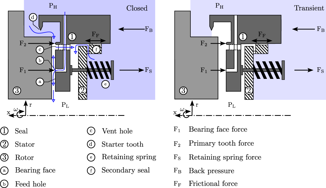
Figure 1 shows a representative schematic of an adaptive face seal design, highlighting the key components, leakage paths and principal forces acting on the seal. The left-hand side of the figure shows the seal in its closed state as it would be during steady-state operation, while the right-hand side shows the seal translated to a partially open state, which corresponds to engine start-up or stop operations. In the case of an axially adaptive seal as shown here, the seal (1) is mounted on the stator (2) by means of a retaining spring (e) and is free to move axially towards or away from the rotor (3). The retaining spring provides an opening force (F
 $_{\textrm {S}}$
), which translates the seal to its fully open position prior to engine start-up, when no pressure difference is applied across the seal. Once the engine is started up and a pressure difference across the seal is established, the back pressure force (F
 $_{\textrm {B}}$
) acts to close the seal. For the seal design presented here, high pressure is applied at the outer radius of the seal, while the low-pressure region is on its inner radius. As the clearance between the starter tooth and the rotor is smaller than the initial bearing face clearance, in the transient regime the pressure drop occurs mainly across the starter tooth. With increasing back pressure, the seal translates towards the rotor until, in the closed position, the gap between the primary tooth and the rotor is smaller than that of the starter tooth, and the pressure drop occurs mainly across the primary tooth. The pressure difference also drives flow through the feed holes (b), which causes a thin, stiff air film to be established between the rotor and the seal bearing face (a). This air film causes additional opening forces F
 $_1$
and F
 $_2$
on the bearing face and the primary tooth, respectively. The typical leakage paths through the seal, shown as arrows in Figure 1, include leakage through the labyrinth configuration of the starter tooth (d) and the primary tooth and out through the vent hole (c), leakage through the feed hole and across the bearing face and leakage through the secondary seal (f). The secondary seal provides an additional frictional force F
 $_{\textrm {F}}$
which opposes any seal movement together with inertial forces of the seal, which are not shown in this schematic. The axial motion of the representative seal is governed by the equation of motion described by Wolfe et al. [Reference Wolfe, Bagepalli, Turnquist, Tseng, McNickle, Hwang and Steinetz2], expressed as
 \begin{equation} \textrm {F}_{ \textrm {B}} - (\textrm {F}_1+\textrm {F}_2+\textrm {F}_{ \textrm {S}}) + \textrm {F}_{ \textrm {F}} = \textrm {m} \ddot {\textrm {x}}. \end{equation}
The air film formed by the feed holes is essential for seal tracking, generating a restorative force that maintains the seal equilibrium position, increasing with decreasing seal clearance and increasing differential pressure.
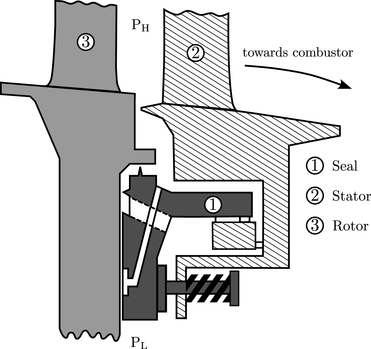
Figure 2 shows a simplified schematic of an adaptive face seal design integrated in a gas turbine, in this case as an axial compressor discharge seal with pocketed feed holes, pressurised radially inwards. The shading in Figure 2 corresponds to that of Figure 1, and the seal (1), stator (2) and rotor (3) are labelled.
Schematic of a representative adaptive face seal, illustrating the principal geometric features and forces (adapted from [Reference Wolfe, Bagepalli, Turnquist, Tseng, McNickle, Hwang and Steinetz2, Reference Bagepalli, Imam, Wolfe, Tseng, Shapiro and Steinetz7], not to scale).

Figure 1. Long description
Panel A: A diagram of an adaptive face seal in the closed position. The seal includes a seal, stator, rotor, bearing face, feed hole, vent hole, starter tooth, retaining spring, and secondary seal. Forces such as bearing face force, primary tooth force, retaining spring force, back pressure, and frictional force are shown. Panel B: A diagram of an adaptive face seal in the transient position. The same components and forces as in Panel A are illustrated, showing the seal in a different operational state.
Schematic of an adaptive face seal employed as an axial compressor discharge seal (adapted from [Reference Moore3], not to scale).

Early experimental work on adaptive face seals includes the publications of Hwang et al. [Reference Hwang, Pope and Shucktis8], Wolfe et al. [Reference Wolfe, Bagepalli, Turnquist, Tseng, McNickle, Hwang and Steinetz2] and Turnquist et al. [Reference Turnquist, Bagepalli, Reluzco, Wolfe, Tseng, McNickle, Dierkes, Athavale and Steinetz9, Reference Turnquist, Tseng, McNickle and Steinetz10].
In one specific application, Hwang et al. state great leakage rate reductions of approximately 80% compared to an equivalent labyrinth seal. Generally, for applications in compressor discharge or turbine inducer locations, they state a potential reduction in specific fuel consumption of 0.5–2.0%. Wolfe et al. [Reference Wolfe, Bagepalli, Turnquist, Tseng, McNickle, Hwang and Steinetz2] describe extensive testing of two seals, including static and dynamic leakage tests, tracking tests, rotor runout and seal tilt tests with and without rotation. They find the seal to provide low leakage and good tracking through axial excursions of 7.62 mm without negative effects in leakage rate.
While the seals are designed for non-contact operation and therefore meant to remain free of wear and maintain constant performance over their lifetime, small sealing gaps can lead to detrimental seal-rotor contact. Although rub events in self-adaptive seals are not well-documented, Turnquist et al. [Reference Turnquist, Bagepalli, Reluzco, Wolfe, Tseng, McNickle, Dierkes, Athavale and Steinetz9] report on one such incident. In their work, they present testing of the larger seal presented in Wolfe et al. [Reference Wolfe, Bagepalli, Turnquist, Tseng, McNickle, Hwang and Steinetz2], including dynamic leakage tests at rotor speeds up to 2,400 rpm, and tests with a seal tilt and rotor runout. For the dynamic leakage testing, they report on a rub incident causing a ‘wiped’ rotor and seal. The seal and rotor faces subsequently required reworking, in which around 80
 $\mu$
m and 1.524 mm of material had to be removed from each part, respectively. During the tests that followed, seal behaviour was found to differ substantially from pre-rub results, leading to the tests being rerun with a new seal and rotor. Although the authors report on the rub event, they give no further details on the possible causes. In a later study, Turnquist et al. [Reference Turnquist, Tseng, McNickle and Steinetz10] describe a second rub incident that occurred during tilt tests of the same seal. At a differential seal pressure of around 6.9 bar and a rotational speed of 2,400 rpm combined with a seal tilt of 0.27
 $^{\circ }$
the rub was detected via an electrical contact probe. The authors report discolouration of the seal over approximately 150
 $^{\circ }$
of its circumference and evidence of light contact on parts of the rotor surface. In this case, rub is attributed to out-of-specification surface finish on the rotor.
Wilhelm [Reference Wilhelm11], describing extensive testing of the transient closing and tracking behaviour as well as the influence of distorted inlet flow and rotor rotation in the context of adaptive seals, reports of seal vibrations possibly caused by a dynamic interaction of aerodynamics and mechanics as well as relative motion of rotor and casing. These seal vibrations, at times occurring at high frequencies and exhibiting a very dynamic behaviour, could result in seal instabilities, later causing rub events.
In mechanical face seals, which are in many aspects similar in design to adaptive face seals, rub events are much more well-documented, with possible causes of contact being rotor runout and inadequate dynamic tracking behaviour between stator and rotor as well as vibrations at off-design conditions [Reference Zhang, Landers and Miller12]. Compared to the abrasive liners commonly used in labyrinth seals, adaptive seals with their much more solid components are not designed for contact operation. Where axial incursion is added on top of the typical radial incursion in labyrinth seals, the seal fins are negatively affected [Reference Lu, Xuan, Ma, Han, Hong and Zhi13].
A rub event in adaptive seals could have detrimental effects on both the seal bearing face and rotor. While contact is expected to result in negative effects ranging from increased leakage to seal failure caused by heat generation and subsequent severe damage to rotating structures, potentially causing total engine failure and therefore representing non-bearable safety issues for jet engines, in adaptive face seals it has so far not been investigated.
This work aims to take a step towards investigating rub events in axially adaptive seals by presenting the overall concept of a modular rig, designed to allow for extended experiments on these events. It presents the rig design allowing for a quick changeover of geometries and material combinations, the measurement capabilities and a detailed error analysis, as well as some preliminary measurements of the air film force of an exemplary seal geometry. Thanks to its extensive measurement capabilities, this rig will help gain new insights on the rubbing process and its effect on the seal and rotor.
2.0 Measurements of the rubbing process in labyrinth seals
The rig presented in this paper is derived from a pre-existing test rig at the Karlsruhe Institute of Technology’s (KIT) Institute of Thermal Turbomachinery (ITS). Previous iterations of the rig have been used for extensive studies on the radial and axial rubbing between labyrinth seal fins and honeycomb stators (see References [Reference Pychynski, Höfler and Bauer14–19]). The most recent study published using the rig involved rubs between seal fins and full honeycomb stator segments [Reference Munz, Hühn, Schwitzke, Bauer, Fischer and Ulan kyzy18]. The test rig allows for the installation of an overhung rotor with a diameter of up to 420 mm, which is driven by an electrical motor with a power of 32 kW and the maximum speed of the rig for radial rubs is around 9,000 rpm. Using a torque-measuring shaft (Lorenz DR-2212) integrated into the drive train, the frictional power of the rub can be measured [Reference Munz, Hühn, Schwitzke, Bauer, Fischer and Ulan kyzy18]. For the investigation of the rubbing process of labyrinth seals against honeycomb liners, the rub is controlled by radially driving the honeycomb stator segment into the rotor, setting a radial incursion depth and speed using a linear traverse with a minimum step size of 0.006 mm while monitoring with a triangulation laser which has a linearity of
 $\pm 7.5$
 $\mu$
m. Axial incursion can be added on top of the radial incursion. To measure the seal-fin temperature, two high-speed pyrometers are used in this setup. They are positioned at 15
 $^{\circ }$
and 30
 $^{\circ }$
behind the rub contact, and, due to their different ranges, enable the measurement of seal fin temperature over a range of 120
 $^{\circ }$
C to 900
 $^{\circ }$
C with an accuracy of
 $\pm 0.4$
K in this setup under the assumption of a constant emission coefficient. The three-dimensional contact forces on the honeycomb stator segment are measured using a piezoelectric force sensor with an accuracy of
 $\pm 0.2$
N in all three directions. All measurements that are recorded during the rub are sampled at a rate of 100 kHz. After the rub, the change in mass and geometry of each honeycomb stator segment is analysed using a precision scale with an accuracy of
 $\pm$
0.48 mg and a two-dimensional laser profile scanner combined with a three-axis traverse. The setup of the laser profile scanner results in a resolution of 25000 px/mm
 $^{2}$
.
3.0 Test rig design
This section details the test rig design with a special focus on the modifications and additions that were made to the pre-existing test rig mentioned in section 2. After stating the rig requirements, a brief overview of the rig is given, and individual subsystems are discussed in detail.
3.1. Rig requirements
A number of modifications and additions are made to the test rig in order to allow for axial rubbing of adaptive face seals. While the concept of the rig, in that a seal segment, from now on referred to as the sample, is pressed against a rotor in a displacement-controlled setup, remains at the core, a number of changes have to be made to allow for measurements of the purely axial rub. Before modifying the rig, the requirements for the axial rub setup were stated as follows:
-
• Axial rub of a sample without damage to the rotor
-
• Simple changeover of samples with various designs
-
• Fine control of sample axial position
-
• Control of alignment between sample and rotor
-
• Measurement of three-dimensional forces on the sample
-
• Setup of an air system to control and measure air flow through the sample
-
• Measurement of sample plenum pressure
-
• Measurement of sample temperature
-
• Measurement of rotor temperature
-
• Prevention of the emission of metal dusts to the surrounding atmosphere
3.2. Rig overview
Figure 3 shows an overview of the test facility including part of the air supply and exhaust systems. At the core of the rig are the rotor assembly and drive train, supported by the base and surrounded by a casing. Opposite the rotor are the sample platform and traverse, on top of which the sample is fixed. The sample is supplied with high-pressure air from the house infrastructure through an air supply system. The sample platform and traverse, the rotor, part of the casing and the final section of the air supply system are encased in a containment, which is connected to a filtered exhaust. The individual subsystems that make up the rig will be described in more detail in the following. While most of the data acquisition is performed on and around the sample platform, some other subsystems are also instrumented. The instrumentation is therefore presented separately along with the data acquisition system and an error analysis.
Overview of the test rig.

3.3. Rig containment and exhaust
The rub process inherently produces fine metal dusts, which will spread throughout the laboratory environment unless countermeasures are taken. To fulfil the rig requirement preventing these emission of metal dusts to the surrounding atmosphere, a rig housing and exhaust system are employed. The housing is made of two parts: a backing plate made from polyvinyl chloride (PVC) placed around the rotor casing at an axial position just behind the rotor and an acrylic glass case mounted on wheels to allow for access to the rig. The antistatic flexible tube connecting the exhaust to the housing is mounted on the left side of the housing so that the rotation of the rotor acts to transport particles towards it. The exhaust provides an adjustable flow rate of up to 1,800
 $\textrm {m}^3$
/hr, capable of renewing the air inside the housing roughly every three seconds and is fitted with an H14 high-efficiency particulate air (HEPA) filter.
3.4. Rotor assembly and drive train
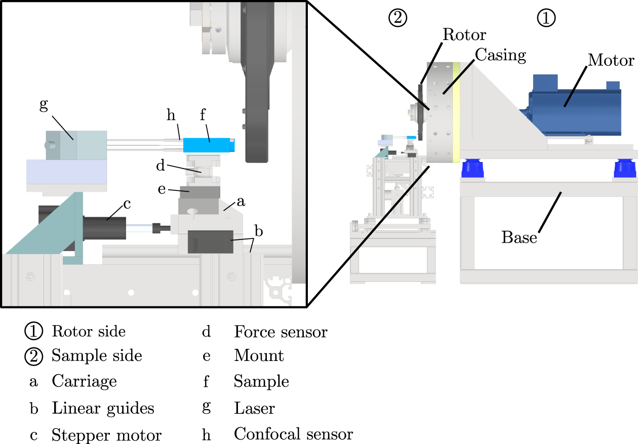
Figure 4 shows an overview of the test facility that is encased in the containment consisting of the rotor (1) and sample (2) sides. On the rotor side, the test rig remains largely unchanged from previous iterations. The rig base, motor and casing are not altered, and the torque-measuring shaft, mentioned in section 2, stays in place. The rotor equipped with seal fins, however, is replaced by a simple rotor disc with an outer diameter of around 380 mm, able to hold insert rings with a mean diameter of around 335 mm and a width of around 21.2 mm. This design allows for an axial rub between the sample and rotor insert ring to occur without damage to the rotor, providing a cost-efficient solution to potentially destructive testing and enables a fast changeover between test runs, allowing for different material pairings and designs.
Overview of the test rig rotor assembly, drive train and sample traverse subsystems.

Figure 4. Long description
Panel 1: A diagram of the rotor side showing a motor attached to a rotor casing. Panel 2: A diagram of the sample side showing a carriage, linear guides, stepper motor, force sensor, mount, sample, laser, and confocal sensor. The carriage is connected to the linear guides and stepper motor. The force sensor is mounted on the carriage, and the sample is placed on the force sensor. The laser is positioned behind the sample and confocal sensor are positioned on the sample so that both measure the position of the sample.
3.5. Sample traverse
The sample side design is modified substantially from previous iterations of the rig to fulfil the requirements of an axial rub experiment (see Figure 4). The actuator of the radial traverse used in previous iterations of the rig [Reference Pychynski, Höfler and Bauer14] is kept in place and now drives a base plate. An axial traverse is implemented on top of the base plate consisting of an aluminium carriage (a) mounted on a pair of linear guides (b) driven by a linear stepper motor (c) with a minimum step size of around 0.0031 mm, allowing for fine control of the sample axial position. Atop the aluminium carriage, a piezoelectric-type 3D force sensor (d) with a variable measurement range (Kistler 9327C), providing measurements of the three-dimensional forces on the sample, is connected through a mount (e). The sample (f) is mounted directly onto the force sensor and will be described in detail later on. The axial and radial positions of the traverse are monitored using laser triangulation sensors, where the axial position laser is labelled (g) and three high-accuracy confocal sensors (h) mounted directly in the sample can be used to measure the relative position of the sample to the rotor and therefore also enable a precise alignment between sample and rotor. As the rig has to be operated from a control room due to safety precautions, the rub can be observed remotely using a standard webcam mounted on the side of the rig next to the axial traverse setup, which is not shown in the figure. Also not shown in the figure is the Sensortherm Metis HI16 high-speed single-wavelength pyrometer, which is positioned on the sample platform base plate pointing at the rotor insert at approximately 30
 $^{\circ }$
behind the centre point of the rub contact. The pyrometer fulfils the rig requirement of measuring the rotor temperature.
3.6. Air supply
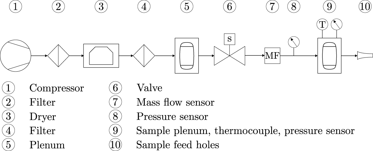
To allow for a realistic measurement of the rub process in an adaptive face seal, an air supply system is required that can control and measure the air flow to the bearing face of the sample. For this, air is supplied by the in-house infrastructure of the institute at a pressure between 5 and 10 bar. The air flow to the sample is controlled using a pneumatic magnet valve paired with a Samson 4763 positioner and measured by means of a downstream calorimetric mass flow sensor, specially calibrated for low mass flows, as well as a gauge pressure sensor installed in the air supply pipe just downstream of the mass flow sensor. The mass flow sensor can measure between 0 and
 $\sim 6.6$
g/s while the pressure sensor has a range of 0-6 bar. Just upstream of the sample plenum, air temperature is measured using a class 1, type K thermocouple, while measurements of sample plenum pressure are taken using a second gauge pressure sensor with a range of 0-5 bar. Figure 5 shows a schematic of the air supply setup.
Schematic of the air system.

3.7. Sample design and alignment
One of the most essential parts of the test rig is the sample, the bearing face test piece used in the axial rub, with a large number of bearing face designs presented literature. Here, a generic groove design was chosen due to the high load capacity and air film stiffness, as well as good stability associated with these types [Reference Gao, Chen, Lu, Huo and Cheng20]. However, as the rig is designed to destructively test a large number of seal segments in order to obtain statistically relevant data on the rub process, it allows for a fast change-over in seal segments and therefore the simple and efficient testing of designs of varying shapes and sizes.
For all preliminary tests presented in this paper, the sample bearing face segment size was chosen as a 15
 $^{\circ }$
segment with five feed holes spaced at 3
 $^{\circ }$
intervals. A seal segment was chosen over a full annular ring for several reasons: first, the pre-existing rig and cost associated with major modifications mean that fitting a full annular seal would be impractical. Second, with axial rubbing being expected to be caused by vibrations of the seal, a fully annular contact is not necessarily the most likely event. Third, the alignment of a full annular seal is more difficult to control and would lead to reduced accuracy in the desired rub location.
Air is supplied to the sample through the in-house infrastructure in the setup mentioned above and shown in Figure 5. Inside the sample, air is first fed into a plenum which in turn supplies the feed holes. The plenum serves the purpose of slowing down the air and providing a constant pressure to the feed holes. Inside the plenum, air temperature and gauge pressure are monitored. Three 0.5 mm diameter class 1, type K thermocouples are placed at spacings of 6
 $^{\circ }$
1.5 mm below the surface of the bearing face to measure sample temperature. Four vent holes at spacings of 3
 $^{\circ }$
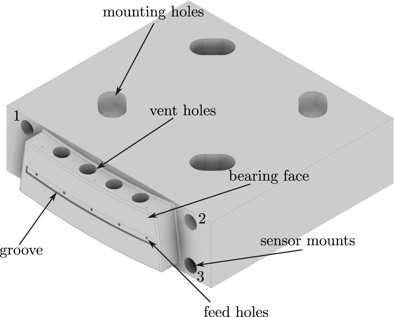
are also included in the bearing face design in order to allow for a more realistic distribution of heat flux throughout the segment upon rub. No other sealing features, such as a starter tooth or primary tooth, are added to prevent additional unwanted contact with the rotor during rub. Figure 6 shows the sample with its key design features.
Sample key design features.

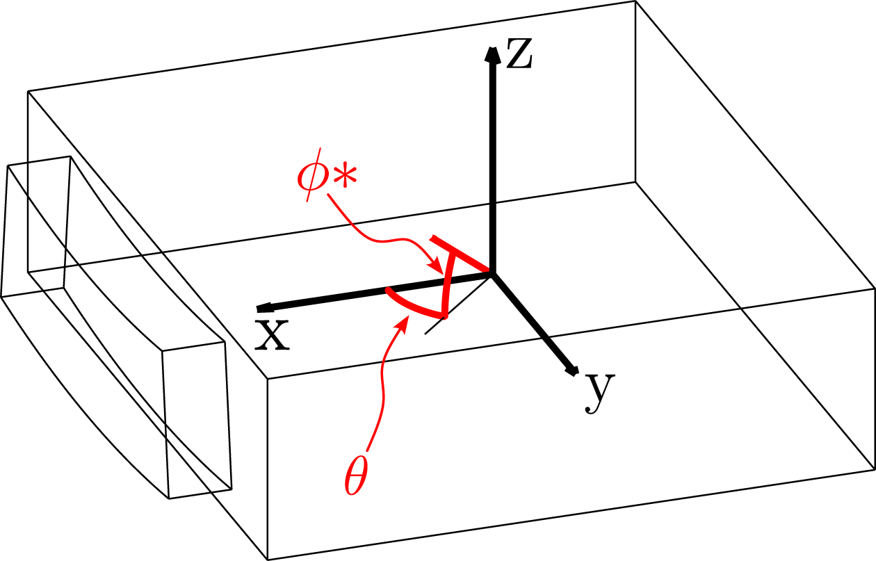
The aft part of the sample, connecting the sample to the force sensor below, is another integral part of the rig setup. It needs to support the sample and enable precise control over the alignment between the rotor and sample surfaces. For initial tests, a parallel alignment, resulting in a flat contact between the sample and rotor, is desired. This is to establish a baseline for comparison, while future tests could include rotations and tilts of the sample to investigate different modes of contact between the seal and rotor. The sample is connected to the force sensor through four bolts and in the sample the holes for said bolts are of an oblong shape and arranged in a circular pattern such that the sample can rotate by
 $\pm$
5
 $^{\circ }$
on the force sensor. This rotation is defined by the angle
 $\theta$
in Figure 7, while the angle labelled
 $\phi *$
in the same figure defines an upward tilt of the sample. Using these two angles, the position of the sample relative to the rotor can be uniquely defined. Three confocal sensors (Micro-Epsilon IFS2402-1,5) are mounted in the sample at the positions 1–3 shown in Figure 6 to measure the distance from the bearing face to the rotor in order to ensure parallelism or establish a desired angle between the surfaces. Using the three confocal sensors and assuming the sample surface is entirely flat, the normal vector of the sample bearing face can be found and hence
 $\theta$
and
 $\phi *$
can be computed. Translations of the sample along the
 $x$
and
 $z$
-axis, as defined in Figure 7, are controlled by the axial and radial traverses mentioned previously, and translations along the
 $y$
-axis can be controlled manually by sliding the force sensor together with its mount by means of oblong holes. This approach assumes a runout-free, plane rotor which, in reality, is not the case. Rotor runout is reduced as much as possible by tight manufacturing tolerances and is measured with a dial gauge prior to sample alignment and tests. The pre- and post-processing protocols of rub samples also remain unchanged compared to previous iterations of the rig, with the same precision scale and two-dimensional profile laser being used.
Sample orientation coordinates.

3.7.1. Alignment process
Precise alignment of the sample to the rotor is of great importance, as poor repeatability would exacerbate the scatter in the already highly unsteady experimental data, which is expected for rub tests. Before any tests, the sample is therefore aligned to the rotor using the procedure described in the following. First, the sample is mounted on the force sensor, with the mounting bolts loosely tightened. Using the axial traverse, the sample is then driven in the positive
 $x$
-direction towards the rotor until it makes contact, when it begins to rotate and align with the rotor surface. Movement in the axial direction continues until a certain force threshold is recorded by the force sensor. The mounting bolts are then tightened to arrest the sample in the aligned position. Using the confocal sensors mounted in the sample, alignment is then verified. Coning is not considered explicitly in this setup, but shims are available in increments of 0.01 mm, which can be used between the force sensor and sample to raise its front or back if required. Shims can also be placed at points between the sample and rotor to produce an angled alignment. For all later aerodynamic tests of the seal, the gap width is defined as the distance between the seal segment and the rotor with values increasing as the seal moves axially away from the rotor in the direction of negative
 $x$
in Figure 7. The sample position at which the gap width is zero, and therefore the seal and rotor are just in contact, has to be re-defined each time the sample is mounted anew. This is done by driving the seal segment into the rotor again and finding the point at which the force in the axial direction rises upon seal-rotor contact. While for theoretical considerations the rotor is considered to be free of axial rotor runout, in reality this runout will result in an imperfect alignment between the sample and the rotor. The axial runout of the rotor is measured using a dial gauge with an accuracy of 5
 $\mu$
m prior to alignment and tests, and the sample is aligned on the flattest part.
Preliminary static air bearing tests as described later on are then performed at this location. The sample zero position at which the sample is just in contact with the rotor is then found at the point with the highest axial runout in order to prevent any undesired contact between the rotor and sample. The true incursion into the rotor at each angular position can then be measured using the confocal sensors and is taken as the mean value over one rotation.
3.8. Measurement system and error estimates
This section describes in more depth the comprehensive measurement system of the rig, implemented to measure forces on the bearing face, mass flow rate of supplied air, static pressures, temperatures, seal position and clearance as well as rotor shaft torque. First, an overview is given overof all measurements, followed by an in-depth discussion of the measurement system, including a description of the data acquisition system, sensor types and configurations, as well as error estimates presented.
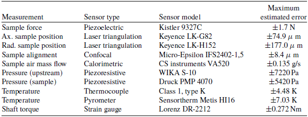
Table 1 shows an overview of the key measurements taken, the instrument type and model utilised, as well as their maximum expected error in this specific setup. The values in Table 1 account for the whole measurement chain, including the data acquisition system as discussed in the following.
Maximum estimated errors for each measured quantity in the test rig

Table 1. Long description
The table presents an overview of key measurements, sensor types, sensor models, and their maximum estimated errors. It has 10 rows and 4 columns. The columns are labeled Measurement, Sensor type, Sensor model, and Maximum estimated error. The rows list various measurements such as Sample force, Ax. sample position, Rad. sample position, Sample alignment, Sample air mass flow, Pressure (upstream), Pressure (sample), Temperature, and Shaft torque. Each row provides details on the sensor type and model used for each measurement and the corresponding maximum estimated error.
The reference temperature in the laboratory changes depending on the environmental conditions, but can be monitored during individual tests to get a more accurate error estimate. Its mean lies around 18
 $^{\circ }$
C, which is the value assumed for the computations leading to the results in Table 1. The control room reference temperature remains constant at around 20
 $^{\circ }$
C through an air conditioning unit.
3.8.1. Data acquisition system
Data acquisition is performed by means of six NI-9215 modules with a range of
 $\pm 10$
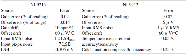
V and one NI-9212 thermocouple module with two internal cold-junction compensators. All data acquisition modules are mounted in a NI cDAQ-9188 chassis. An overview of the two module types used and their associated errors can be found in Table 2.
Typical errors for calibrated NI-9215 and NI-9212 modules at temperatures between + 18 °C and + 28 °C

Table 2. Long description
A table comparing typical errors for calibrated NI-9215 and NI-9212 modules. The table has two main sections, one for NI-9215 and one for NI-9212, each with columns for Source and Error. For NI-9215, the sources and errors are: Gain error (percent of reading) 0.02, Offset error (percent of range) 0.014, Gain drift 10 ppm/C, Offset drift 60 V/C, Input RMS noise 1.2 LSB, Input pk-pk noise 7 LSB, LSB 0.305 mV. For NI-9212, the sources and errors are: Gain error (percent of reading) 0.02, Offset error 5 V, Input RMS noise 1 V RMS, Offset drift 60 V/C, Temperature measurement 0.05 C, accuracy/sensitivity, Cold-junction compensation accuracy 0.25 C.
Each data acquisition module has a number of potential error sources, including gain and offset errors, gain and offset drifts associated with temperature, as well as input noise and analogue-to-digital conversion errors associated with the resolution.
No details are given by the manufacturer on the method of determining the input noise quoted, but it is assumed that it includes the analogue-to-digital conversion precision error. The reference temperature for both modules on which the thermal drift is to be calculated is 23
 $^{\circ }$
C and the sampling frequencies of the modules are set to 100 kHz and 95 Hz for the NI-9215 and NI-9212 modules, respectively, corresponding to the maximum possible values. As the sampling frequency for both modules is set to high values and measurements are taken over comparatively long amounts of time, the computation of the errors introduced by the data acquisition modules neglects the precision errors (input noise and analogue to digital conversion error) as those two errors are truly statistical and will reduce with the number of samples taken, while also being comparatively small. For the relevant settings employed on the NI-9212 in this test rig the manufacturer claims all measurement errors of the module and terminal block to typically range between
 $\pm$
0.39
 $^{\circ }$
C –
 $\pm$
0.48
 $^{\circ }$
C for the relevant temperature ranges and with a maximum error of around
 $\pm 1.68$
 $^{\circ }$
C. Relevant temperature ranges here are taken up to 700
 $^{\circ }$
C, but might be lower, hence resulting in a lower total error in the thermocouple measurement.
3.8.2. Instrumentation and measured quantities
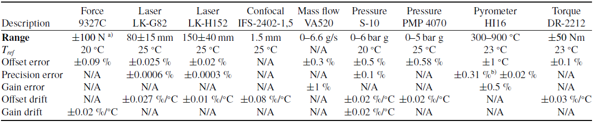
This section describes the key instrumentation installed in the test rig as well as the information obtained from the manufacturers on which the error estimates in Table 1 are based. Table A1 in the appendix shows the errors quoted in the data sheets categorised by constant offset and gain errors, where the percentage data are given relative to the end value of the range and the measured value, respectively, if not indicated otherwise. Although arguments for neglecting precision errors in the computation of the total estimated errors have been given in the previous section, they are included in the table for the sake of completeness.
The force sensor utilised is a Kistler 9327C piezoelectric type, which requires a charge amplifier type 5080A. The available force sensor range depends on the position of installation and of a single sensor where the force is applied directly through the surface of its top cover spans
 $\pm$
1,000 N in the axial and tangential directions and
 $\pm$
8,000 N in the radial direction. In practice, however, the available ranges are diminished by a combination of various maximum moments around the centre point of the sensor, which may not be exceeded. The manufacturer provides information on the measurement error in the data sheet by quoting a sensor linearity (which includes sensor hysteresis) of
 $\leq \pm$
0.5 % of the full-scale output, as well as a crosstalk between the tree sensor channels of
 $\leq \pm$
3 % or
 $\leq \pm$
1 % of the measured value, where the channels in the axial and tangential directions have a higher influence on the other channels than the one in the radial direction. To achieve a more accurate estimate of the error, the manufacturer also supplies calibration values for each individual sensor. In the case of this sensor, the most recent calibration yielded linearity values of
 $\pm$
0.09 % of the full-scale output and a crosstalk of
 $\leq \pm$
2.3 % or
 $\leq \pm$
0.8 % of the measured value. In addition to these sources of error, there is an inherent electrical drift of approximately
 $\pm 0.05$
pC/s, which is combatted by discharging the sensor before each measurement process and therefore taking the force measurement relative to a starting condition. A temperature-dependent drift of the sensor signal is also considered, where the offset drift can be neglected due to the discharging of the sensor before each measurement and the gain drift is quoted to be approximately
 $\pm 0.02$
%/
 $^{\circ }$
C. Dynamic temperature errors, i.e. errors due to the sensor temperature not being in thermal equilibrium with the environment, are also considered by the manufacturer, but neglected here as all measurements are taken relative to the start of the experiment and sensor temperature is not expected to change. Still, an additional thermocouple is used to monitor sensor temperature during the measurements in order to correct for this error if necessary. The charge amplifier contributes an additional drift and a measurement uncertainty of around
 $\le \pm$
0.03 pC/s and
 $\le \pm$
0.6 %. The full-scale output of the sensor is variable and can either be taken as
 $\pm$
100 N or
 $\pm$
1,000 N by selecting the respective charge sensitivity in the calibration sheet of the sensor.
The two laser triangulation sensors used to measure the axial and radial position of the sample traverse are a Keyence LK-G82 and Keyence LK-H152 laser head, respectively, both connected to suitable control units. The lasers have ranges of
 $\pm 15$
mm at an offset distance of 80 mm and
 $\pm 40$
mm at an offset distance of 150 mm, and the manufacturer quotes any errors with respect to the entire system of laser head and control unit. For both laser sensors, as well as the force sensor that comes with a signal conditioner provided by the manufacturer, the errors given include the entire system as it is set up before the data acquisition module.
The three confocal sensors are of the type IFS2402-1,5 by Micro-Epsilon. Two of the sensors are operated with an IFC2422 controller and one with an IFC2461 by the same manufacturer, where each controller is specifically calibrated to work with the individual sensors. This leads to an error of
 ${\le \pm 1.2\ \mu\ \text{m}}$
in the entire measurement chain up to the output of the controller plus a temperature-dependent offset drift of
 $\pm 1.2$
 $\mu$
m/
 $^{\circ }$
C.
Mass flow to the rig is measured with the calorimetric mass flow sensor VA520 of CS instruments. As this sensor has a current output, it is connected to the data acquisition system through a signal conditioner (MINI MCR-SL-I-U-4), which is also taken into account in Table 1. The range of the signal conditioner is 4-20 mA and the manufacturer quotes a maximum offset error of
 $\pm$
0.1% of the end range value as well as a temperature dependent offset drift of
 $\pm$
0.01% of the end range per degree Celsius of temperature change at a reference temperature of 22.5
 $^{\circ }$
C.
Pressure is measured at the location of the mass flow sensor as well as in the sample plenum with two piezoresistive gauge pressure sensors of the types WIKA S-10 and Druck PMP 4070 with measurement ranges of 0–6 and 0–5 bar and a 0–10 V output signal.
Temperature measurements of the air inside the sample plenum as well as the bearing face material at three separate locations 1.5 mm below the sample bearing face are performed with class 1, type K thermocouples. As the errors introduced in thermocouples are expressed differently to the other instrumentation, they are not included in Table A1. According to DIN EN 60584-1:2014-07 [21], class 1 thermocouples have an error of
 $\pm 1.5$
 $^{\circ }$
C over the range −40
 $^{\circ }$
C to + 375
 $^{\circ }$
C and
 $\pm$
0.4 % of the measured value over the range between + 375
 $^{\circ }$
C and + 1,000
 $^{\circ }$
C.
During the rub, the rotor insert temperature is measured using a high-speed single-wavelength pyrometer with a spectral range of 1.45–1.8
 $\mu$
m; however, this measurement is expected to provide only a qualitative comparison between runs, due to the difficulties associated with pyrometer measurements in this particular setting. Pyrometers are passive, contactless temperature measurement devices whose operational principle is based on the infra-red energy radiated by the measured object at a given temperature. For a grey body at a temperature,
 $T$
, greater than absolute zero, the spectral radiance it emits per unit wavelength is governed by Planck’s law (see, for example, References [Reference Caniou22, Reference Marr and Wilkin23])
 \begin{equation} I_\lambda = \frac {\varepsilon C_1}{\lambda ^5 \exp\!(C_2/(\lambda T))-1}, \end{equation}
where
 $C_1 =1.191 \times 10^{14}$
Wm
 $^{-3}$
sr
 $^{-1}$
 $\mu$
m
 $^{5}$
and
 $C_2$
= 1.439
 $\times 10^4$
 $\mu$
mK, are the first and second radiation constants, respectively,
 $\lambda$
is the wavelength and
 $\varepsilon$
is the body’s emissivity, which therefore needs to be known to correctly determine its temperature. While usually, in infra-red thermography the surfaces to be measured are coated with black paint in order to raise emissivity, this is not practical for rub testing. An a-priori calibration through measurements of insert temperature through a different instrument combined with pyrometer measurements is also currently outside the scope of work, as the emissivity of a body depends on its material, temperature and surface finish, as well as the pyrometer wavelength, meaning the results of a pyrometer measurement might change throughout the rub process. Therefore, for the purposes of this test rig, the inserts will be treated as a black body with emissivity equal to one, which leads to a consistent underestimation of their temperature. As direct optical access to the insert is required, the pyrometer also only measures insert temperature at a point behind the rub contact, resulting in a cooling of the insert in the time between contact with the stator segment and the measurement of temperature [Reference Pychynski15]. The time interval between contact and measurement depends on the pyrometer position, as well as the rotor size and speed. In Reference [Reference Pychynski15], the transient cool-down of flash temperatures on a rotor seal fin after rub is described using an exponential function and a dependency on geometry, material and convective cooling properties is stated. The pyrometer operated in this test rig is also connected to the data acquisition system via a MINI MCR-SL-I-U-4 signal conditioner, transforming the 4–20 mA current output to a 0–10 V signal. While the precision errors for pyrometer measurements performed with the Sensortherm Metis HI16 in this test rig are of comparable scale to the other errors quoted for this instrument, they are omitted in the calculation for consistency, and the special case of temperature measurements using the pyrometer will be treated in the following.
Shaft torque is measured with a Lorenz DR-2212 strain gauge type sensor. The sensor has a measurement range of
 $\pm$
50 Nm corresponding directly to its analogue output at
 $\pm$
5 V.
3.8.3. Computation of error estimates
To analyse the full errors induced by the measurement system, one has to take into account the entire measurement chain, including the sensor, any signal conditioners and the data acquisition modules with their respective gains
 $k_n$
. Generally, it can be assumed that each part,
 $n$
, of the measurement chain potentially introduces an additional constant error
 $\epsilon _{C,n}$
and a gain error
 $\epsilon _{G,n}$
, which also amplifies all previous errors. Here, the constant error
 $\epsilon _{C,n}$
includes any offset errors, hysteresis and non-linearity errors. Figure 8 shows the measurement chain for a general case, including the true input signal, sensor, signal conditioner, data acquisition module and the measured signal that is recorded. The analysis is simplified by assuming steady signals taken over a significant time frame.
Example of a generic measurement chain with three nodes.

At each stage,
 $n$
, the signal,
 $y_n$
, can be expressed as
 $y_n=y_{n-1}k_n+\epsilon _n$
, where
 $\epsilon _n=y_{n-1}k_n\epsilon _{G,n}+\epsilon _{C,n}$
. Using the expressions
 $a_n = (1+\epsilon _{G,n})k_n$
and
 $b_n=\epsilon _{C,n}$
, and defining the initial condition as
 $y_0=x$
,
 $y_n$
can be expressed as
 \begin{equation} y_n = x\prod _{i=1}^{n}a_i+ \sum _{j=1}^{n} b_j \prod _{l=j+1}^{n} a_l, \end{equation}
where the product of
 $a_l$
is empty for
 $j=n$
, i.e.
 $\prod _{i=m}^{n} x_i=1$
if
 $m\gt n$
. The total accumulated error at each stage
 $n$
can thus be expressed as
 \begin{equation} \epsilon _n = y_n - x\prod _{i=1}^{n}k_i = x\,\bigg (\prod _{i=1}^{n}a_i-\prod _{i=1}^{n}k_i \bigg )+ \sum _{j=1}^{n} b_j \prod _{l=j+1}^{n} a_l, \end{equation}
again, making use of the empty product for
 $j=n$
. The maximum error introduced through the measurement chain can be estimated by assuming
 $x$
, the true value of the measured quantity, to be at the top of the instrument measurement range and then computing the expression given in Equation (4).
Derived quantities. While most quantities are measured directly, derived quantities might be of interest when analysing the obtained data. Two examples of derived quantities of interest are the air bearing film stiffness, i.e. the derivative of force on the seal segment due to the air film established between seal and rotor with respect to seal clearance and the total rub power, i.e. the rub torque times the rotor angular velocity.
For a derived quantity
 $y$
, which can be expressed in terms of independent measured quantities
 $x_1,x_2,x_3,\ldots , x_n$
where each
 $x_i$
has a known error
 $\Delta x_i$
, the error in
 $y$
resulting from
 $\Delta x_i$
can be expressed as
 \begin{equation} \Delta y_i = y(x_1,x_2,x_3,\ldots ,x_i+\Delta x_i,\ldots ,x_n)-y(x_1,x_2,x_3,\ldots ,x_n). \end{equation}
Under the assumption of small errors, a Taylor series expansion can be applied and retaining only the first derivatives leads to the expression
 \begin{equation} \Delta y_i = \frac {\partial y}{\partial x_i}\Delta x_i. \end{equation}
Depending on whether signed errors are given, the expression of the total error hence either result in
 \begin{equation} \Delta y = \sum _{i=1}^{n}\frac {\partial y}{\partial x_i}\Delta x_i \end{equation}
or
 \begin{equation} \Delta y = \sum _{i=1}^{n}\bigg | \frac {\partial y}{\partial x_i} \bigg | \Delta x_i. \end{equation}
The often-quoted error-propagation formula of Gaussian error propagation, as well as the error propagation rule of Kline and McClintock [Reference Kline and McClintock24], assumes each of the variables
 $x_1, \ldots , x_n$
to be normally distributed and are therefore, strictly speaking, only applicable to the analysis of precision errors, not bias errors such as linearity and hysteresis [Reference Mills and Chang25].
4.0 Preliminary tests
This section presents the preliminary results of a number of initial air bearing and rub tests performed to characterise rig behaviour.
4.1. Alignment and air bearing tests
While the test rig is not specifically designed to analyse the performance of varying air bearing designs under engine-relevant conditions; for example, by measuring leakage mass flow, it can be used to compare the aerodynamic performance of the air bearing before and after the rub event. For this, the force on the bearing face surface is measured for a given pressure drop across the seal. The performance of the air bearing can be analysed dynamically or statically, and under rotating or static rotor conditions. As the air bearing force is closely linked to the seal bearing face design [Reference Gao, Cheng, Chen, Ding and Fu26], this additional type of measurement is of great significance and allows further investigate the effect of rub on the stability of the seal.
In preliminary testing, air bearing force is measured for the seal geometry presented in section 3.7 under static rotor conditions at two choked and two unchoked operating points. The air bearing force is normalised by the total area of the sample and the differential pressure across the seal:
 \begin{equation} \tilde {\textrm {F}} = \frac {\textrm {F}_{\textrm {BF}}}{\textrm {A}_{\textrm {BF}}(\textrm {P}_{\textrm {in}}-\textrm { P}_{\textrm {out}})}, \end{equation}
as presented in Reference [Reference Zimmermann, Guemmer, Nguyen and Giepman27]. The distance to the rotor is normalised by the feed hole radius:
 \begin{equation} \tilde {\textrm {x}} = \frac {\textrm {x}_{\textrm {BF}}}{\textrm {r}_{\textrm {FH}}}, \end{equation}
and the pressure difference across the seal is normalised by a reference pressure:
 \begin{equation} \Delta \textrm {P} = \frac {(\textrm {P}_{\textrm {in}}-\textrm {P}_{\textrm {out}})}{\textrm {P}_{\textrm {ref}}}. \end{equation}
While the reference pressure in Reference [Reference Zimmermann, Guemmer, Nguyen and Giepman27] is unknown, in this case a constant pressure of 1 bar is used as the reference pressure.
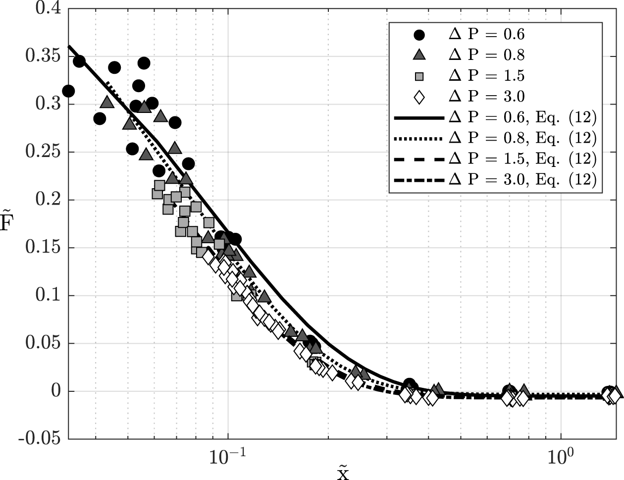
Figure 9 shows the normalised air bearing force,
 $\tilde {\textrm {F}}$
over the normalised axial distance to the rotor
 $\tilde {\textrm {x}}$
for four different pressure levels, where
 $\Delta$
P = 0.6 and
 $\Delta$
P = 0.8 are unchoked conditions, while
 $\Delta$
P = 1.5 and
 $\Delta$
P = 3.0 are choked. Choked flow is considered where the ratio of stagnation pressure in the plenum to outlet pressure is larger than or equal to 1.893, while unchoked flow is considered for pressure ratios below 1.893. The critical pressure ratio is derived from isentropic flow assumptions for dry air at 20
 $^{\circ }$
C but is validated individually for each presented measurement. Air temperatures measured in the sample plenum vary between
 $\sim$
16 – 18
 $^{\circ }$
C. The sample alignment was not changed between the measurements, and the values for
 $\theta$
and
 $\phi *$
as described in section 3.7 lie around 0.049
 $^{\circ }$
and −0.044
 $^{\circ }$
, showing values of tilt and coning lying in very similar ranges. The tilt is the result of an imperfect alignment between the sample and rotor with respect to rotations around the z-direction in Figure 7 and would result in a stronger rub on the leading edge of the bearing face. The coning is the result of a combination of axial runout of the rotor in the radial direction at the measured position and horizontal positioning of the sample with respect to the rotor. For the coning presented in this instance, contact between the rotor and seal would be first made at the lower radius of the seal.
Normalised air bearing force over normalised axial distance to the rotor for four different pressure levels.

In Figure 9, it can be seen that under the influence of air flow through the seal, smaller axial gap widths could be reached for lower values of
 $\Delta$
P due to the stiffness of the sample side of the rig. Overall, it can be seen that under both choked and unchoked conditions, the shape of the graph agrees very well. For large distances to the rotor of around
 $\tilde {\textrm {x}}\gt$
0.3, the measured force on the bearing face becomes negative in some cases, turning the bearing face force from an opening force into a closing force. In some cases, this might act to de-stabilise the system; however, it must be noted that for all negative measurements the horizontal line of
 $\tilde {\textrm {F}}$
= 0 lies within the measurement uncertainty. For all pressure levels, the absolute values of
 $\tilde {\textrm {F}}$
agree very well, which initially suggests that there is no optimum in bearing face performance for a given pressure in this design and the absolute bearing face force increases roughly linearly with the differential pressure across the seal. The overall shape of the curve can be modelled as
 \begin{equation} \tilde {\textrm {F}} = a \exp (\!-b\tilde {\textrm {x}})+c, \end{equation}
for both choked and unchoked conditions. The model is represented by black solid, dotted, dashed and dot-dash lines in the figure for the respective pressures. The coefficients
 $a$
and
 $c$
remain roughly constant for all four pressure levels, with
 $a$
lying between 0.53 and 0.58 and
 $c$
lying between
 $\sim$
−0.0032 and −0.0068. The scaling coefficient
 $b$
, however, lies between
 $\sim$
11.4 and 15.0 and increases with
 $\Delta$
P. This increase suggests a faster decay in
 $\tilde {\textrm {F}}$
with
 $\tilde {\textrm {x}}$
for higher seal pressures, which contradicts the previous observation and suggests decreased seal stability at higher pressures. The value of the coefficient of determination,
 $R^2$
, lies above 98% for
 $\Delta$
P
 $\geq$
0.8, and above 96% for
 $\Delta$
P
 $=$
0.6. This poorer fit at the lower pressure level is caused by the higher spread of the data at very small seal clearances for the lowest pressure.
4.2. Rub tests
To analyse rig performance, five initial rub tests were performed, the results of which are reported here.
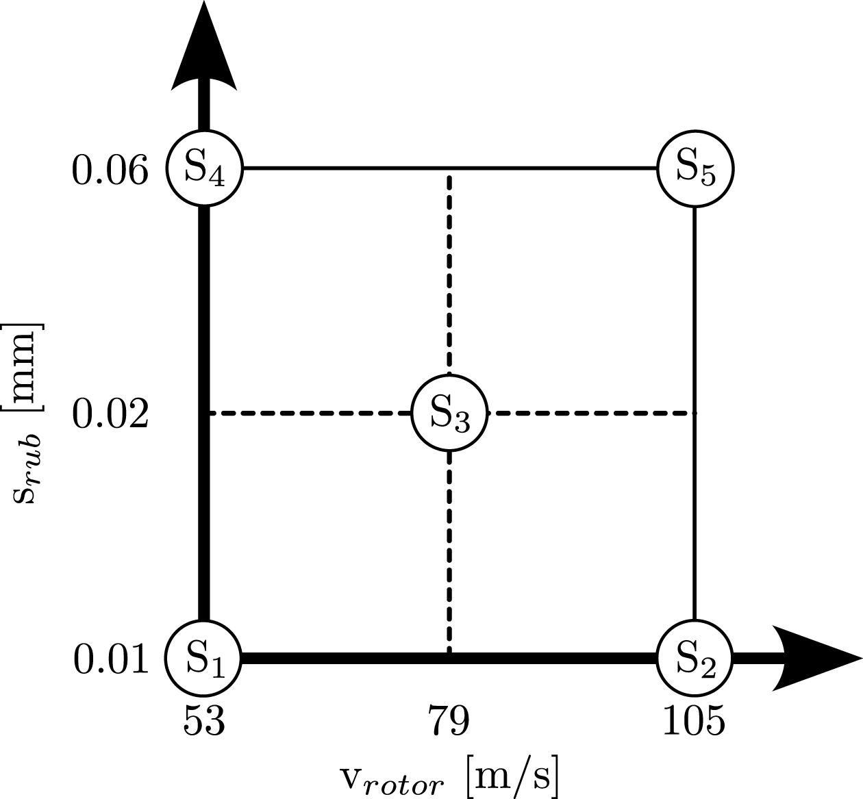
The sample design used in the tests presented here is the one shown in section 3.7, and the design was manufactured from X5CrNi18-10 stainless steel. The initial tests were performed according to the test matrix shown in Figure 10, with rotor speeds (
 $\textrm {v}_{rotor}$
) and incursion depths (
 $\textrm {s}_{rub}$
) varying, while the axial incursion rate was set to a constant. Small incursion depths were chosen in order to achieve minimal wear of the sample and allow for repeat use. The sample was aligned once and
 $\theta$
and
 $\phi *$
were found to be around 0.017
 $^{\circ }$
and 0.0066
 $^{\circ }$
. In absolute terms, both values are low, indicating a good overall alignment of the sample. Positive values of
 $\theta$
would result in initial contact on the segment leading edge, leading to an uneven rub and locally higher contact pressures. Positive values of
 $\phi *$
would lead to initial contact between rotor and segment at the outer radius of the segment. At the very low values of
 $\theta$
and
 $\phi *$
presented here, the orthogonality of the sample surface and sensor mounting holes would have to be taken into account. Using the solenoid valve described in section 2,
 $\Delta$
P was set to a value of 1.5 at the test starting position defined at 0.5 mm away from the rotor. After sample alignment, positioning and mass flow setup, the test was started by driving the sample into the rotor at the predefined incursion speed until the desired incursion depth was achieved, while acquiring measurement data through the system described in section 3.8. After reaching the desired incursion depth, the sample was retracted automatically.
Test matrix for initial rub tests.

Figure 11 shows the time-resolved three-dimensional forces on the seal segment for test
 $S_3$
represented as contact pressures. The representation as contact pressures is achieved by normalising the recorded forces by the seal segment bearing face area. The signal can be divided up into two regions: the force resulting from the air bearing labelled
 $a)$
, and the force resulting from contact to the rotor, labelled as region
 $b)$
in the figure. In the case of the test presented here, the seal segment comes into contact with the rotor at around
 $t = 4.3$
s, as marked by a solid vertical line (1) on the graph. Prior to that, the influence of the air bearing on the axial force is clearly visible, with pressure on the segment rising with time and hence decreasing distance to the rotor. Upon contact with the rotor, the contact pressure continues to rise, although the rate of change of the increase in pressure decreases shortly after contact as the rotor provides some resistance to the axial motor. As the axial motor begins to retract the segment, marked by a dashed line (2), the contact pressure drops sharply, reducing back down to zero as first contact between the segment and rotor is lost (marked by another solid line (3)) and then the influence of the air bearing becomes negligible with increasing distance to the rotor. Overall, the axial contact pressure rises up to a maximum level of around 0.125 MPa in this case, which can be seen in more detail in Figure 12. Contact pressures in tangential and radial directions remain low, peaking at around 0.075 and 0.01 MPa, respectively. The influence of the air bearing in the radial direction is likely an artefact of the increased crosstalk in the sensor channels from axial to radial directions, as discussed in section 2.
Time-resolved data of the measured contact pressures in axial, tangential and radial directions.

Time resolved data of the measured contact pressure in the axial direction.

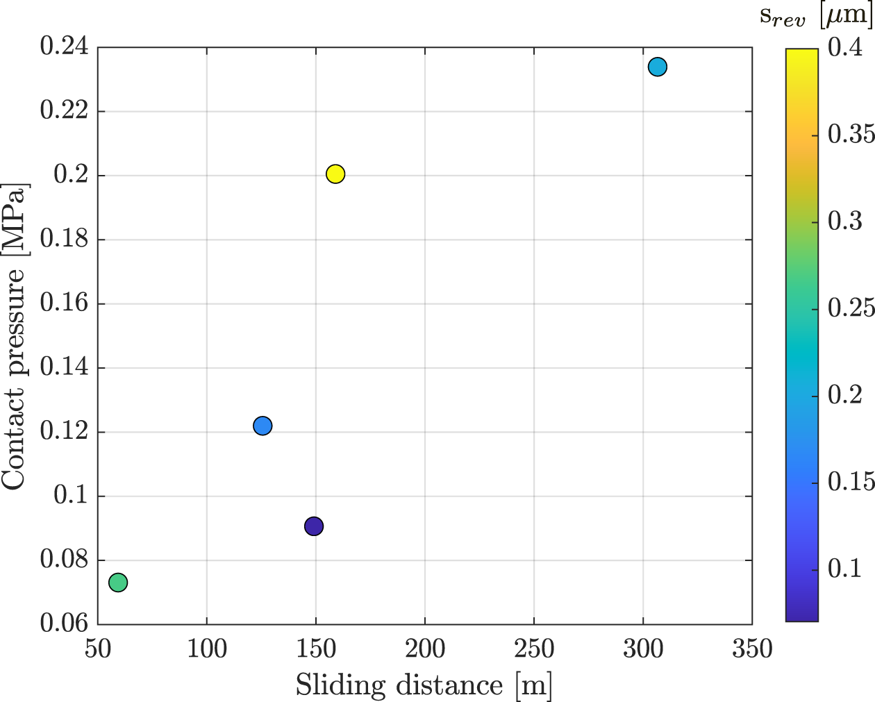
Figure 13 shows the contact pressure of all five tests versus the total sliding distance, defined as the product of rub time and rotor speed [Reference Hühn, Munz, Schwitzke and Bauer17]. In each case, the markers are coloured by
 $s_{rev}$
, the ratio of incursion rate to rotor speed, i.e. the incursion per revolution. Contrary to the observations in Reference [Reference Hühn, Munz, Schwitzke and Bauer17], the contact pressure rises with sliding distance in the experiments presented here. This suggests low overall wear and high component strength, likely due to low surface temperatures caused by heat conduction away from the sample and rotor. No conclusive trend can be observed with regards to
 $s_{rev}$
. Overall, the sliding distance and contact pressures achieved in the tests presented here are small compared to the ones presented in radial rub tests with foils (see References [Reference Pychynski, Höfler and Bauer14, Reference Hühn, Munz, Schwitzke and Bauer17]), due to the much smaller incursion depths and much larger segment area present in this case. Future tests should include higher incursion depths as well as a large number of repeat tests using a large number of samples.
Contact pressure as a function of sliding distance. The colour map indicates
 $\textrm {s}_{rev}$
, the incursion per revolution.

5.0 Conclusions and future work
This paper presents a novel test rig for investigating axial rubbing of adaptive face seals, enabling characterisation of air bearing performance, wear behaviour and transient thermal response, as well as assessment of aerodynamic stiffness of the bearing face flow before and after rubbing events. The rig provides operation over a wide range of relevant conditions through independent control of rotational speed, incursion depth and rate and seal mass flow.
The modular design of the rig, extending to both rotor and sample assemblies, allows for a rapid changeover between geometries and material combinations while preserving rotor integrity and reducing overall test cost. This flexibility, combined with the available instrumentation, allows detailed aerodynamic and mechanical characterisation of seal behaviour under controlled operating conditions. Prior to rubbing, the rig enables measurement of bearing face forces as a function of differential pressure and seal gap width, providing insight into the aerodynamic performance of a given seal design.
Preliminary aerodynamic results show an approximately linear relationship between bearing face force and differential pressure for the investigated geometry. Repeating this characterisation after rub events may provide further insight into changes in seal stability and performance degradation mechanisms. Initial rub tests conducted on a single seal segment indicate an increase in contact force with sliding distance, suggesting limited wear under the initial test conditions. However, the observed scatter in the data highlights the stochastic nature of the rubbing process and the need for repeat testing to improve statistical confidence.
The in-test thermal measurement capabilities as well as the capability to quantify wear post-test through two-dimensional laser scanning and high-precision mass measurements, enabling a detailed assessment of surface topography changes and mass loss, were presented, but a detailed discussion of these aspects lies outside the scope of the present article. A detailed uncertainty analysis of the measurement system was also conducted to support interpretation of the experimental results.
Future work will focus on systematic parameter studies varying operating conditions and material combinations to develop a more comprehensive understanding of the rubbing process and its effects on both the seal and rotor surfaces. This will support the development of adaptive face seals with improved robustness under contact conditions.
Competing interests
The authors declare none.
Appendix
A.1 Error overview
Overview of the different types of error quoted for the instrumentation on the rig

Table A1. Long description
The table presents a comparison of different types of errors for various instruments used in a test rig. It includes columns for Force 9327C, Laser LK-G82, Laser LK-H152, Confocal IFS-2402-1,5, Mass flow VA520, Pressure S-10, Pressure PMP 4070, Pyrometer HI16, and Torque DR-2212. Each row provides details on range, reference temperature, offset error, precision error, gain error, offset drift, and gain drift. For example, the Force 9327C has a range of ±100 N, a reference temperature of 20 °C, an offset error of ±0.09 percent, and a gain drift of ±0.02 percent/°C. The table aims to provide a comprehensive overview of the error estimates for each instrument.
 $^{\textrm {a)}}$
Variable range, value used for calculations;
 $^{\textrm {b)}}$
Precision error here given as 0.2 % gain plus 1
 $^{\circ }$
C offset.




 srev

 Open access

