1. Introduction
1.1 This paper is the next in a series that updates the Wilkie model, originally put forward in Wilkie (Reference Wilkie1986) and Wilkie (Reference Wilkie1995), and follows Part 1 (Wilkie et al., Reference Wilkie, Şahin, Cairns and Kleinow2011), Part 2 (Wilkie & Şahin, Reference Wilkie and Şahin2016), Parts 3A, 3B and 3C (Wilkie & Şahin, Reference Wilkie and Şahin2017a, Reference Wilkie and Şahin2017b, Reference Wilkie and Şahin2017c) and Part 4 (Wilkie & Şahin, Reference Wilkie and Şahin2018). In Part 4 we observed that in the model for retail prices there was a correlation with wages, which we had not allowed for, between the residuals of the inflation rate model in any year, and the residuals of the wages model in the previous year, which suggested that a vector autoregressive (VAR) model might be appropriate. We investigate this suggestion in this paper.
1.2 The first reason for having modelled the retail prices index (RPI), Q, without reference to the wages index, W, was that in the first version of the model in Wilkie (Reference Wilkie1986), a wages index was not included, being of less immediate importance than those variables that were modelled. It was included in Wilkie (Reference Wilkie1995), because it was thought to be necessary for the valuation of pension schemes with salary-related benefits, and possibly for assessing future liability claims in general insurance and in future wage and salary expenses in any organisation. These advantages still apply.
1.3 However, some users of stochastic models (now often called Economic Scenario Generators) may consider that wages are an unnecessary complication of the model, and making them essential, as we do in this paper, is an undesirable feature.
1.4 Another consideration is that good international figures for average earnings are not readily available. Some countries seem to prefer to publish indices of hourly wage rates in manufacturing industry, which is a useful statistic for a different purpose than pension funds would require. We do not consider other countries in this paper.
1.5 In section 2 we state the basic formula that we use. In section 3 we give estimation results. In section 4 we discuss further calculations and show the long-term means and variances, and the correlation coefficients, comparing them with those of the original model. In section 5 we show certain results for forecasting. In section 6 we consider stochastic interpolation. In section 7 we show specimen forecasts. In section 8 we draw some conclusions. We put almost all the algebra into the Appendix.
2. Formulation
2.1 The original Wilkie model for retail prices, Q(t), with parameters QMU, QA and QSD, is:
 $$\eqalignno{ & I\left( t \right)\,{\equals}\,{\rm ln}\left( {Q\left( {t{\plus}1} \right)} \right)-{\rm ln}\left( {Q\left( t \right)} \right) \cr & IN\left( t \right)\,{\equals}\,I\left( t \right)-QMU \cr & QE\left( t \right)\,{\equals}\,QSD.QZ\left( t \right) \cr & I\left( t \right)\,{\equals}\,QA.IN\left( t \right){\plus}QMU{\plus}QE\left( t \right) \cr & Q\left( {t{\plus}1} \right)\,{\equals}\,Q\left( t \right).{\rm exp}\left( {I\left( t \right)} \right) $$
2.2 The fuller form of the original model for wages, W(t), with parameters WMU, WW1, WW2, WA and WSD, is:
 $$\eqalignno{ & J\left( t \right)\,{\equals}\,{\rm ln}\left( {W\left( {t{\plus}1} \right)} \right)-{\rm ln}(W\left( t \right)) \cr & JN\left( t \right)\,{\equals}\,J\left( t \right)-WW1.I\left( t \right)-{\rm }WW2.I\left( {t-1} \right){\rm }-WMU \cr & WE\left( t \right)\,{\equals}\,WSD.WZ\left( t \right) \cr & J\left( t \right)\,{\equals}\,WW1.I\left( t \right){\plus}WW2.I\left( {t-1} \right){\plus}WMU{\plus}WA.JN\left( t \right){\plus}WE\left( t \right) \cr & W\left( {t{\plus}1} \right)\,{\equals}\,W\left( t \right).{\rm exp}\left( {J\left( t \right)} \right) $$
Often WA could be taken as 0, so the term WA.JN(t) could be dropped out.
2.3 To include dependence of I(t) on J(t–1) we could elaborate the formula for I(t) which we shall put in the form, changing the constant term from QMU to QM:
 $$I\left( t \right)\,{\equals}\,QA.I\left( {t-{\rm }1} \right){\plus}QW.J\left( {t-{\rm }1} \right){\plus}QM{\plus}QE\left( t \right)$$
But this suggests that a full symmetrical VAR model might be appropriate so we put:
 $$J\left( t \right)\,{\equals}\,WQ.I\left( {t-1} \right){\plus}WA.J\left( {t-1} \right){\plus}WM{\plus}WE\left( t \right)$$
with a correlation coefficient, QWR, between QZ(t) and WZ(t). All the parameters for this can be estimated jointly. We assume throughout that QZ(t) and WZ(t) are distributed as unit normal, N(0, 1), although there is good evidence that the residuals are fatter tailed than normal.
2.4 It is convenient to replace QMU in formula (1) by QM in formula (3), since this allows us to estimate the parameters of (3) without reference to the model for W, though the data for W(t) is still used. We can then adjust formula (4) to:
 $$J\left( t \right)\,{\equals}\,WQ.I\left( {t-1} \right){\plus}WA.J\left( {t-1} \right){\plus}WM{\plus}WBQ.QE\left( t \right){\plus}WSD2.WZ\left( t \right)$$
Where the correlation is incorporated in the WBQ term and WSD is adjusted to WSD2. See Appendix A1.1. The parameters for formula (5) can then be estimated after formula (3) has been fitted.
2.5 Formulae (3) and (4) or (3) and (5) are convenient for estimation, but for future simulation and other calculations it is convenient to re-arrange them as:
 $$I\left( t \right)\,{\equals}\,QA.IN\left( {t-1} \right){\plus}QW.JN\left( {t-1} \right){\plus}QMU{\plus}QE\left( t \right)$$
 $$J\left( t \right)\,{\equals}\,WQ.IN\left( {t-1} \right){\plus}WA.JN\left( {t-1} \right){\plus}WMU{\plus}WBQ.QE\left( t \right){\plus}WSD2.WZ2\left( t \right)$$
with IN(t)=I(t)−QMU and JN(t)=J(t)−WMU:
We can derive the values of QMU and WMU (see Appendix A2) from:
 $${{QMU\,{\equals}\,\left\{ {\left( {1-WA} \right).QM{\plus}QW.WM} \right\}} \mathord{\left/ {\vphantom {{QMU\,{\equals}\,\left\{ {\left( {1-WA} \right).QM{\plus}QW.WM} \right\}} {\left\{ {\left( {1-WA} \right).\left( {1-QA} \right)-QW.WQ} \right\}}}} \right. \kern-\nulldelimiterspace} {\left\{ {\left( {1-WA} \right).\left( {1-QA} \right)-QW.WQ} \right\}}}$$
 $${{WMU\,{\equals}\,{\rm }\left\{ {WQ.QM{\plus}{\rm }\left( {1{\rm }-QA} \right).WM} \right\}} \mathord{\left/ {\vphantom {{WMU\,{\equals}\,{\rm }\left\{ {WQ.QM{\plus}{\rm }\left( {1{\rm }-QA} \right).WM} \right\}} {\left\{ {\left( {1{\rm }-WA} \right).{\rm }\left( {1{\rm }-QA} \right){\rm }-QW.WQ} \right\}}}} \right. \kern-\nulldelimiterspace} {\left\{ {\left( {1{\rm }-WA} \right).{\rm }\left( {1{\rm }-QA} \right){\rm }-QW.WQ} \right\}}}$$
3. Estimation
3.1 We have the annual June values of the RPI and its predecessors, and the Average Weekly Earnings Index (seasonally adjusted) from June 1921 to June 2016. We use these as Q(t) and W(t). This gives us annual values of I(t) and J(t) from 1922 to 2016, and we fit the model to the 94 values from 1923 to 2016, using the values for June 1922, in the formulae for 1923. We use maximum likelihood estimation, assuming normally distributed residuals. This gives the same estimates of the values of the parameters as least squares, but also gives us standard errors (and covariances) for all the parameters.
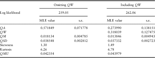
3.2 We start by estimating the parameters for formula (3), but omitting the term QW.JN(t−1). This is the same as the present model, but QM has a different value from QMU. The results are shown in Table 1. We then include the omitted term, so that the results are now the same as with the joint, VAR, model. These results are also shown in Table 1. The improvement in log likelihood is significant at 3.01 and the extra term is also significantly different from 0. But the improvement is not enormous.
Maximum likelihood estimation (MLE) parameter values and standard errors (s.e.) for models for Q.

3.3 We show the skewness and kurtosis in Table 1. Both are large, for both models. This indicates that it is not correct to assume that the residuals are normally distributed, but we postpone investigating this until a later Part in this series.
3.4 We show at the foot of Table 1 the value of QMU, the long-term mean value of I(t). For the model omitting QW, QMU can be calculated as QM/(1−QA). For the VAR model, including QW, it cannot be calculated until we also have the model for wages too, and then from the formula in section 2.5. The values of QMU are not the same, but are not very far apart.
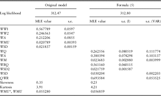
3.5 We now do the same for the wages model, showing in Table 2 the results, first for the original model, and then for the new VAR model. This can be estimated either on its own, after the model for Q has been fitted, or jointly with the model for Q. The estimated values of the parameters are the same, except that for the joint model we obtain two different parameters, WSD and QWR, which are essentially the same as WBQ and WSD2 (see Appendix A1). The sum of the log likelihoods of the individual models is numerically the same as the (algebraically more complicated) log likelihood of the joint model. But the standard errors of the parameter estimates in the wages model differ, being larger in the joint model than in the individual one. This is presumably because in the joint model the values of the standard deviations, QSD and WSD, and the correlation coefficient, QWR, are estimated jointly, whereas in the individual wages model the values of QSD and the QE(t) terms are taken as fixed and only the parameter WBQ has to be estimated. In Table 2 we show the two standard errors as “s.e. (I)” for the individual model and “s.e. (VAR)” for the joint model. The standard errors in the model for Q are unaffected.
Maximum likelihood estimation (MLE) parameter values and standard errors (s.e.) for models for W.

Note: VAR, vector autoregressive.
3.6 The skewness and kurtosis for the two models are also shown. These are not so large as for the model for Q, but still cast some doubt on the assumption of normally distributed residuals.
3.7 We show also at the foot of Table 2 the values of WMU*, the long-term mean value of J(t). For the original model this is calculated as WMU+(WW1+WW2).QMU. For the VAR model it is calculated from the formula in section 2.5 for WMU. (We call it WMU* to avoid confusion with WMU in the original model that might be better called WM.)
3.8 The log likelihood for the two models is almost the same, that for the VAR model being 0.33 higher than for the original model, a trivial improvement. The same three connections are included. For the original model I(t) is included directly; for the VAR model it is connected through the correlation with QZ(t) or the WBQ.QE(t) term. I(t–1) is included directly in both models, and the estimates of the parameters, WW2 and WQ have quite similar values. J(t–1) is included directly in the VAR model, and indirectly through WA.JN(t–1) in the original model. The estimates of the parameters, called WA in both models, are rather different.
3.9 In aggregate the only improvement of the VAR model over the present one is in the model for Q. This is large enough to make it worthwhile using this model, at the expense of making the wages model essential, rather than an optional extra, and making the calculation of expected values and variances of future forecasts rather more complicated, as we see in section 4.
4. Forecast means and variances
4.1 For further calculations, for both the original models and the new VAR model, we round the parameter estimates shown in Tables 1 and 2 to four decimal places. We also adjust the values of the means QMU and WMU. We assume that QMU=0.0250, as we did in Part 4 (Wilkie & Şahin, Reference Wilkie and Şahin2018), since that seems a more suitable value in current conditions, than the historic means of 0.0423 and 0.0440. For WMU we observe that WMU is 0.0130 greater than QMU for the old model and 0.0129 greater for the new model, so we choose a mean rate of wages growth of 0.0380 for both models. We put WMU=0.0380 for the new model, but for the old model, we need an adjustment to give WMU=0.01764. For the new model we also, for some purposes, use formula (5) for which we need WBQ and WSD2 instead of WSD and QWR, but to get consistent results we calculate values for these from the rounded values and use more decimal places.
4.2 Thus for the new model we use:
 $$\eqalignno{ & QA\,{\equals}\,0.2740,QW\,{\equals}\,0.3180,WQ\,{\equals}\,0.2626,WA\,{\equals}\,0.3804, \cr & QSD\,{\equals}\,0.0373,WSD\,{\equals}\,0.0302,QWR\,{\equals}\,0.6936 \cr & QMU\,{\equals}\,0.0250,WMU\,{\equals}\,0.0380 \cr & WBQ\,{\equals}\,0.56157426,WSD2\,{\equals}\,0.02175489 $$
For the old models we use:
 $$\eqalignno{ & QA\,{\equals}\,0.5718,QMU\,{\equals}\,0.0250,QSD\,{\equals}\,0.0385 \cr & WW1\,{\equals}\,0.5678,WW2\,{\equals}\,0.2466,WA\,{\equals}\,0.2122,WMU\,{\equals}\,0.01764,WSD\,{\equals}\,0.0218 $$
4.3 In Part 2 we discussed the state variables, input and output variables, and initial conditions required for simulation. These remain almost the same, except that in the old model, the value of I(–1) was required in order to calculate JN(0), and it is no longer required for that purpose. However, it is required for other variables in the total model.
4.4 We wish to calculate the means, variances and covariances of future values of I(t), QL(t), J(t) and WL(t), conditional on the starting position at some time where we take t=0. For numerical examples we use both neutral initial conditions and initial conditions as at June 2016. The initial conditions affect the means, but not the variances and covariances. This is all as shown in Part 2, but the formulae are more complicated for the VAR model. The algebra is discussed in Appendix A3. We also calculate the corresponding values for the present model. We show here only the results.
4.5 Neutral initial conditions for both old and new models are to put I(0)=QMU=0.025, W(0)=(or WMU*)=0.038. The initial conditions as at June 2016 are:
 $$I\left( 0 \right)\,{\equals}\,0.0161,I\left( {-1} \right)\,{\equals}\,0.0101,Q\left( 0 \right)\,{\equals}\,263.1,J\left( 0 \right)\,{\equals}\,0.0216,W\left( 0 \right)\,{\equals}\,156.7.$$
We need I(–1) for the old model in order to calculate JN(0). For some purposes it is more convenient to use arbitrary values for Q(0) and W(0) such as 1.0, since these are multiplicative indices.
4.6 The long-term means and standard deviations of I(t) and J(t) are shown in Table 3: The means of each are the same for both models, because we have made them so. The standard deviations of each for the new model are a little lower than for the old, and in both cases the standard deviation for J(t) is lower than for I(t). The long-term correlation coefficient between I(t) and J(t) is very slightly lower in the new model. In total there is not very much difference.
Long-terms means and standard deviations (s.d.) of I(t) and J(t), and correlation coefficient (CC) between I(t) and J(t)

Note: VAR, vector autoregressive.
5. Forecasting
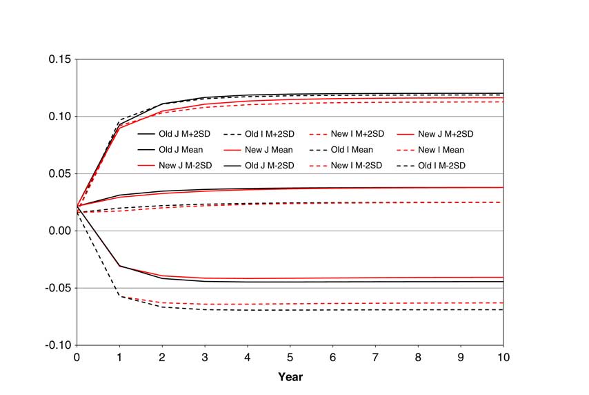
5.1 Using the formulae in the Appendix we calculate the means (formulae A1–A4) and standard deviations (formulae A5–A8 give the variances) of I(t), J(t), QL(t) and WL(t), for both the original model and the new VAR model We use the initial conditions as at June 2016. In Figure 1 we show the means and the means plus and minus twice the standard deviations of the forecast values of I(t) and J(t). If we assume normality of the innovations, this spread gives roughly a 95% confidence interval for the forecasts.
Mean and mean±2× standard deviation, for I(t) and J(t) for both the old and new models.

5.2 We go ahead only 10 years, by which time all the values have converged almost to their long-term values. We show the old model with black lines, the new with red, and show the values for J(t) as solid lines, and for I(t) as dashed ones. The long-term means for both models are the same, because we made them so; our purpose is to show the spread. Consistent with the numbers in Table 3, the new model shows a slightly narrower spread than the old; more so for I(t) than J(t). Also the spread for I(t) is greater than that for J(t).
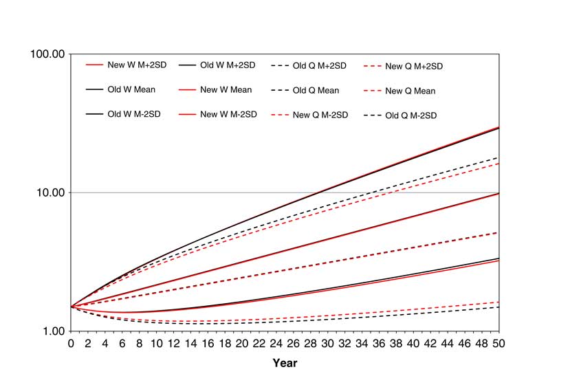
5.3 We do the same for QL(t) and WL(t), and then exponentiate to give the equivalent values of Q(t) and W(t). The result strictly does not give the mean values of Q(t) and W(t), because, if we assume normality of the innovations, Q(t) and W(t) would be lognormally distributed, and what we call the mean is strictly the median; but the spread is still a 95% one. We show the results in Figure 2, for 50 years ahead. Since this is on a logarithmic vertical scale it shows in effect QL(t) and WL(t) on a linear scale. We choose arbitrary starring values for both Q(0) and W(0) of 1.5, in order to keep the results within two cycles of the scale.
Mean and mean±2× standard deviation, for Q(t) and W(t) for both the old and new models.

5.4 The relative positions of the lines are the same as in Figure 1. The new model shows a slightly narrower spread than the old, and the spread for I(t) is greater than that for J(t).
6. Stochastic Interpolation
6.1 In Parts 3A, 3B and 3C we discussed stochastic interpolation, using Brownian bridges to obtain monthly values of QL(t,m) and WL(t,m), the simulated values in month m of year t. We update our analysis from June 2014 to June 2016, but the extra two years make little difference to the results. However, we observe that, in fitting the annual model, we start with I(1923), which is calculated from QL(1922) and QL(1923), so it is more consistent to use the monthly values starting from June 1922, giving one extra year at the beginning. For wages we explained in Part 3B why we could not start the monthly analysis till June 1934, and we do the same here. Thus we analyse QL for the 94 years from 1922 to 2016, and WL for the 82 years from 1934 to 2016.
6.2 For QL the monthly standard deviation for year t varies with the change in QL(t) over the year, QLD(t), which equals I(t+1), and the best formula is the same as before:
 $$\sigma _{m} \left( t \right)\,{\equals}\,QSM\left( t \right)\,{\equals}\,QSA{\plus}QSB{\times}{\rm Abs}\left( {QLD\left( t \right)-QSC} \right)$$
but with slightly altered parameters QSA=0.004177, QSB=0.055982 and QSC=0.03933. The correlation coefficient is 0.5963, not very different from the previous 0.5865. The correlation coefficient between the standardised forward deviations for corresponding months in successive years is 0.5491, a small change from 0.5469 previously.
6.3 For WL we get a similar result, with rather little change from previously. The most suitable formula is still:
 $$\sigma _{m} \left( t \right)\,{\equals}\,WSM\left( t \right)\,{\equals}\,WSA{\plus}WSB{\times}{\rm Abs}\left( {WLD\left( t \right)} \right)$$
with WSA=0.002513 and WSB=0.011482. The correlation coefficient is 0.3188, a small increase on the previous 0.2826. The correlation coefficient between the standardised forward deviations for corresponding months in successive years is 0.1933, a small change downwards from 0.2047 previously.
7. Simulations
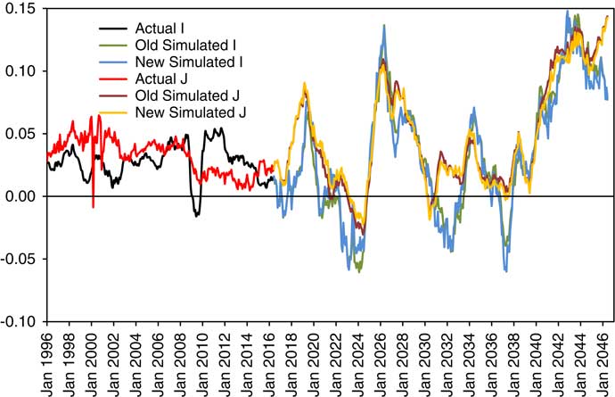
7.1 We are now in a position to simulate these variables for a chosen period ahead. In Figure 3 we show, first the actual values of I(t) and J(t), monthly, from January 1996 to June 2016. Note that I(t) and J(t) are the values of the changes in QL(t) and WL(t) over the preceding year, not over one month. Then we have done simulation of I(t) and J(t) on two bases, the old and the new, from which we calculate simulated values of QL(t) and WL(t). We than apply stochastic interpolation over QL(t) and WL(t), using Brownian bridges as described in section 6; and from these we calculate values for I(t) and J(t) for intermediate months. We use the same random unit normal innovations for both the old and the new model.
One pair of simulations, on both the old model and new model, for I(t) and J(t) showing 20 years of past data and 30 years of simulated future values.

7.2 We show the past actual data in black and red lines, and the simulated futures in other colours. We can see that the two models give quite similar future values. This is only one pair of simulations, and they may not be “typical” (if any single simulation can be thought to be typical). They show larger deviations of both variables, both upwards and downwards than the recent past data, but the upwards range is much less than that of the further back past, of the 1980s or the 1920s.
8. Conclusions
8.1 There are advantages and disadvantages of the new VAR model as compared with the old. The log likelihood for I(t) in the VAR model is rather higher, and the resulting standard deviation, QSD, rather smaller than for the old model, so it can be said to describe the data better. However, the change for W(t) is small. The VAR model is symmetrical, and is a standard time series model; but the old model is a normal transfer function model. Either model is straightforward to simulate, but one must note that the old “cascade-style” model can be simulated either variable by variable for a given number of years, or year by year for all variables. The VAR model requires one to proceed year by year.
8.2 With the VAR model, the formulae for forecast means and variances are more complicated than for the original model. We have not shown the formulae for all the other variables which depend on I(t), as we did in Part 2, but the complications spread everywhere.
8.3 The results for the new model are not very different from those using the old one, and one may well feel that a change in any existing system is not worth the trouble. But for someone starting a new development we would, on balance, recommend the VAR one.
Appendix
A1 Equivalence of formulae (4) and (5)
A1.1 In section 2.4 we state that formula (5) for J(t) is equivalent to formula (4). The formulae are the same except for the ending terms. Formula (4) ends with WE(t), which equals WSD.WZ(t), and there is correlation of QWR between WZ(t) and QZ(t). Formula (5) ends with WBQ.QE(t)+WSD2.WZ2(t), and WZ2(t) is assumed to be independent of QZ(t). The equivalence is easily shown if we consider the Choleski decomposition of the correlation matrix:
 $$M\,{\equals}\,\left[ {\matrix{ 1 & {CQW} \cr {CQW} & 1 \cr } } \right]$$
which is
 $$C\,{\equals}\,\left[ {\matrix{ 1 & 0 \cr {CQW} & {\sqrt {1{\minus}CQW^{2} } } \cr } } \right]$$
and C.C T =M, so that C is, in a sense, the square root of M.
We now put WBQ=QWR.WSD/QSD and
 $$WSD{\rm 2\,{\equals}\,}WSD{\rm .}\sqrt {1{\minus}CQW^{2} } $$
.
A1.2 For both formulae the terms we are considering are the only stochastic ones, and in both cases the expected value is 0. The formula (4) term is WSD.WZ(t) and the variance of this is WSD 2. The corresponding stochastic part of I(t), in formula (3) is QSD.QZ(t). The covariance of I(t) and J(t) is therefore QSD.WSD.Cov[QZ(t).WZ(t)]=QSD.WSD.QWR.
A1.3 We expand formula (5) to give:
 $$WBQ.QSD.QZ\left( t \right){\rm \lsquo {\plus}}WSD2.WZ2\left( t \right){\rm \,{\equals}\,}QWR.WSD.QZ\left( t \right){\plus}WSD.\sqrt {1{\minus}CQW^{2} .} WZ2\left( t \right)$$
The variance of this is:
 $$\eqalignno{ \left( {WBQ.QSD} \right)^{2} {\plus} WSD2^{2} \,{\equals}\,&\left( {QWR.WSD} \right)^{2} {\plus}WSD^{2} .\left( {1{\rm }-QWR^{2} } \right) \cr \,{\equals}\, & WSD^{2} .{\rm }\left( {QWR^{2} {\plus}1{\rm }-QWR^{2} } \right) \cr \,{\equals}\, & WSD^{2} $$
which is the same as the variance in formula (4). The covariance between J(t) with formula (5) and I(t) is QWR.WSD.QSD, which is also the same as in formula (4).
A1.4 In our estimation for the period 1923–2016 with the VAR model we get QSD=0.037322, WSD=0.030204 and QWR=0.693584 (see Tables 1 and 2). We can calculate from the formulae above that WBQ=QWR.WSD/QSD=0.561160 and also that WSD2=WSD.
 $\sqrt {1{\minus}CQW^{2} } $
=0.021759, which agree exactly with those parameters estimated with the individual model. Using our rounded values for the parameters we get WBQ=0.056157426, and WSD2=0.02175489.
A2 Calculation of QMU and WMU
A2.1 In section 2.5 we state that formulae (3) and (5) can be transformed to formulae (6) and (7). The formulae are:
 $$I\left( t \right)\,{\equals}\,QA.I\left( {t-1} \right){\plus}QW.J\left( {t-1} \right){\plus}QM{\plus}QE\left( t \right)$$
 $$J\left( t \right)\,{\equals}\,WQ.I\left( {t-1} \right){\plus}WA.J\left( {t-1} \right){\plus}WM{\plus}WBQ.QE\left( t \right){\plus}WSD2.WZ\left( t \right)$$
 $$I\left( t \right)\,{\equals}\,QA.IN\left( {t-1} \right){\plus}QW.JN\left( {t-1} \right){\plus}QMU{\plus}QE\left( t \right)$$
 $$J\left( t \right)\,{\equals}\,WQ.IN\left( {t-1} \right){\plus}WA.JN\left( {t-1} \right){\plus}WMU{\plus}WBQ.QE\left( t \right){\plus}WSD2.WZ2\left( t \right)$$
with IN(t)=I(t)−QMU and JN(t)=J(t)−WMU.
A2.2 Equating corresponding formulae we see that:
 $$QM\,{\equals}\,-{\!}QA.QMU-QW.WMU{\plus}QMU\,{\equals}\,\left( {1-QA} \right).QMU-QW.WMU$$
 $$WM\,{\equals}\,-{\!}WQ.QMU-WA.WMU{\plus}WMU\,{\equals}\,-{\!}WQ.QMU{\plus}\left( {1-WA} \right).WMU$$
From these simultaneous equations we get:
 $$\eqalignno{ & {{QMU\,{\equals}\,\left\{ {\left( {1-WA} \right).QM{\plus}QW.WM} \right\}} \mathord{\left/ {\vphantom {{QMU\,{\equals}\,\left\{ {\left( {1-WA} \right).QM{\plus}QW.WM} \right\}} {\left\{ {\left( {1{\rm }-WA} \right).{\rm }\left( {1{\rm }-QA} \right){\rm }-QW.WQ} \right\}}}} \right. \kern-\nulldelimiterspace} {\left\{ {\left( {1{\rm }-WA} \right).{\rm }\left( {1{\rm }-QA} \right){\rm }-QW.WQ} \right\}}}$$
 $${{WMU\,{\equals}\,{\rm }\left\{ {WQ.QM{\plus}{\rm }\left( {1{\rm }-QA} \right).WM} \right\}} \mathord{\left/ {\vphantom {{WMU\,{\equals}\,{\rm }\left\{ {WQ.QM{\plus}{\rm }\left( {1{\rm }-QA} \right).WM} \right\}} {\left\{ {\left( {1{\rm }-WA} \right).{\rm }\left( {1{\rm }-QA} \right){\rm }-QW.WQ} \right\}}}} \right. \kern-\nulldelimiterspace} {\left\{ {\left( {1{\rm }-WA} \right).{\rm }\left( {1{\rm }-QA} \right){\rm }-QW.WQ} \right\}}} $$
A2.3 For our data we have QA=0.273990, QW=0.318039, WQ=0.262556, WA=0.380294, QM=0.013846 and WM=0.023683, so we get QMU=0.043979 and WMU=0.056859.
A3 Means of forecasts
A3.1 Our methods here are similar to the well-known method of solving for a univariate recurrence relation like:
 $$X_{t} \,{\equals}\,a.X_{t-1} {\plus}b.X_{t-2}$$
where we find the roots, x 1 and x 2, of the characteristic equation:
 $$x^{2} \,{\equals}\,a.x{\plus}b$$
We then put X t =c 1.x 1 t +c 2.x 2 t
And find c 1 and c 2 from any two given values of X t .
A3.2 If we ignore the stochastic parts of the equations for I(t) and J(t) and omit the mean terms we have a bivariate recurrence relation for future expected values:
 $$\eqalignno{ & IN(t)\,{\equals}\,QA.IN\left( {t-1} \right){\plus}QW.JN\left( {t-1} \right) \cr & JN\left( t \right)\,{\equals}\,WQ.IN\left( {t-1} \right){\plus}WA.JN\left( {t-1} \right) $$
We can write this in matrix form as:
 $${\mib{xN}} \left( t \right)\,{\equals}\,{\bf T}.{\mib{xN}} \left( {t-1} \right)$$
where xN (t)=[IN(t), JN(t)]T
 $${\mib{T}} \,{\equals}\,\left[ {\matrix{ {QA} & {{\rm }QW} \cr {WQ} & {WA} \cr } } \right]$$
A3.3 The equivalent of the roots, x 1 and x 2, are the eigenvalues, λ 1 and λ 2, of this matrix, obtained from | T −λ. I |=0
 $$\left| {\matrix{ {QA{\minus}\lambda } & {QW} \cr {WQ} & {WA{\minus}\lambda } \cr } } \right|\,{\equals}\,0$$
 $$\eqalignno{ & \left( {QA-\lambda } \right).\left( {WA-{\rm }\lambda } \right)-QW.WQ\,{\equals}\,0 \cr & \lambda _{1} ,\lambda _{2} \,{\equals}\,{{\{ {( {QA{\plus}WA} \right)\,\pm\,\sqrt {\left( {(QA-WA} \right)^{2} {\plus}4.QW.WQ)} } \right\}} \mathord{/ {\vphantom {{\left\{ {\left( {QA{\plus}WA} \right)\,\pm\,\sqrt {\left( {(QA-WA} \right)^{2} {\plus}4.QW.WQ)} } \right\}} 2}} } 2} $$
For our data we get λ 1, λ 2=0.327192±0.293854 so λ 1=0.654383 and λ 2=0.033366, these are both positive and real, which is convenient. But these are not the only possibilities, as we discuss further in A3.8
A3.4 We assume that we start at time t=0 with initial conditions I(0) and J(0) known. We can then calculate IN(0)=I(0)–QMU and JN(0)=J(0)–WMU. Using formulae (6) and (7) we can calculate E[IN(1)]=QA.IN(0)+QW.JN(0) and E[JN(1)]=WQ.IN(0)+WA.JN(0) and recursively E[IN(t+1)]=QA.IN(t)+QW.JN(t) and E[JN(t+1)]=WQ.IN(t)+WA.JN(t). At this stage we omit all stochastic terms. We have a simple bivariate recurrence relation for E[IN(t)] and E[JN(t)]
A3.5 We now postulate that E[IN(t)]=A1.λ 1 t +A2.λ 2 t and E[JN(t)]=B1.λ 1 t +B2.λ 2 t . We know E[IN(0)]=IN(0) and we calculate E[IN(1)] as above. We can then put:
 $$E\left[ {IN\left( 0 \right)} \right]\,{\equals}\,A1{\plus}A2$$
and
 $$E\left[ {IN\left( 1 \right)} \right]\,{\equals}\,QA.IN\left( 0 \right){\plus}QW.JN\left( 0 \right)\,{\equals}\,A1.\lambda _{1} {\plus}A2.\lambda _{2} $$
From these we readily get:
 $$\eqalignno{ & {{A1\,{\equals}\,\left\{ {\left( {QA-\lambda _{2} } \right).IN0{\plus}QW.JN\left( 0 \right)} \right\}} \mathord{\left/ {\vphantom {{A1\,{\equals}\,\left\{ {\left( {QA-\lambda _{2} } \right).IN0{\plus}QW.JN\left( 0 \right)} \right\}} {\left( {\lambda _{1} -\lambda _{2} } \right)}}} \right. \kern-\nulldelimiterspace} {\left( {\lambda _{1} -\lambda _{2} } \right)}} \cr & {{A2\,{\equals}\,IN\left( 0 \right)-A1\,{\equals}\,\left\{ {\left( {QA-\lambda _{1} } \right).IN0{\plus}QW.JN\left( 0 \right)} \right\}} \mathord{\left/ {\vphantom {{A2\,{\equals}\,IN\left( 0 \right)-A1\,{\equals}\,\left\{ {\left( {QA-\lambda _{1} } \right).IN0{\plus}QW.JN\left( 0 \right)} \right\}} {\left( {\lambda _{2} -\lambda _{1} } \right)}}} \right. \kern-\nulldelimiterspace} {\left( {\lambda _{2} -\lambda _{1} } \right)}} $$
Then similarly we get:
 $$\eqalignno{ & {{B1\,{\equals}\,\left\{ {\left( {WA-\lambda _{2} } \right).JN0{\plus}WQ.IN\left( 0 \right)} \right\}} \mathord{\left/ {\vphantom {{B1\,{\equals}\,\left\{ {\left( {WA-\lambda _{2} } \right).JN0{\plus}WQ.IN\left( 0 \right)} \right\}} {\left( {\lambda _{1} -\lambda _{2} } \right)}}} \right. \kern-\nulldelimiterspace} {\left( {\lambda _{1} -\lambda _{2} } \right)}} \cr & {{B2\,{\equals}\,JN\left( 0 \right)-B1\,{\equals}\,\left\{ {\left( {WA-\lambda _{1} } \right).JN0{\plus}WQ.IN\left( 0 \right)} \right\}} \mathord{\left/ {\vphantom {{B2\,{\equals}\,JN\left( 0 \right)-B1\,{\equals}\,\left\{ {\left( {WA-\lambda _{1} } \right).JN0{\plus}WQ.IN\left( 0 \right)} \right\}} {\left( {\lambda _{2} -\lambda _{1} } \right)}}} \right. \kern-\nulldelimiterspace} {\left( {\lambda _{2} -\lambda _{1} } \right)}} $$
A3.6 The proof by induction that, if E[IN(t)]=A1.λ 1 t+A2.λ 2 t then E[IN(t+1)]=A1.λ 1 t+1+A2.λ 2 t+1 is tedious, and relies on the fact that λ 1 and λ 2 are the roots of the quadratic in λ, so that λ 1+λ 2=QA+WA and λ 1.λ 2=QA.WA–QW.WQ. There is a similar formula for E[JN(t)].
A3.7 We can now, given the relevant values of IN(0) and JN(0), readily calculate E[IN(t)] and E[JN(t)] for any t, and hence also E[I(t)] and E[J(t)], which are:
 $$E\left[ {I\left( t \right)} \right]\,{\equals}\,A1.\lambda _{1}^{t} {\plus}A2.\lambda _{2}^{t} {\plus}QMU$$
 $$E\left[ {J\left( t \right)} \right]{\rm }\,{\equals}\,B1.\lambda _{1}^{t} {\plus}B2.\lambda _{2}^{t} {\plus}WMU$$
We see also that as t→∞, E[IN(t)] and E[JN(t)] → 0, hence E[I(t)] → QMU and E[J(t)] → WMU. These results depend on |λ 1|<1 and |λ 2|<1, which is true in our case.
A3.8 In A3.4 we noted that λ 1 and λ 2 were both are positive and real, but that there were other possibilities with different data. Since, with different data, we would expect to have different parameter estimates, then we might have one of the roots greater than unity, so the system would be divergent rather than mean-reverting. If the square root part were a little larger, we might get λ 2 negative, which is not much trouble, since the formulae are the same, except that the effect of λ 2 t alternates between positive and negative. But if λ 2 remains small, then the terms in λ 2 t reduce very rapidly, and the dominant effect is that of λ 1. If λ 2 were exactly 0, then the transition matrix would be singular, and there would be a problem in identifying the parameters uniquely. Another possibility is that the term inside the square root is negative so the roots are a complex conjugate pair. We have not explored this fully, but the algebra would be the same, with complex numbers throughout, and the effect would probably be that the forecast values would lie on a damped sine wave.
A3.9 The forecast means for I(t) and J(t) have formulae analogous to those for I(t) in the original model, as shown in Part 2, except that we have terms with powers of λ 1 and λ 2 instead of terms in QA In Appendix A2.2 of that paper we had:
 $$E\left[ {QL\left( t \right)} \right]\,{\equals}\,QL\left( 0 \right){\plus}t.QMU{\plus}QA.{\rm SumGS}\left( {QA,t} \right).IN\left( 0 \right)$$
where SumGS(x, t)=1+x+x 2+ … +x t–1=(1–x t )/(1–x)
We can then put, in our case:
 $$E\left[ {QL\left( t \right)} \right]\,{\equals}\,QL\left( 0 \right){\plus}t.QMU{\plus}A1.\lambda _{1} .{\rm SumGS}\left( {\lambda _{1} ,t} \right){\plus}A2.\lambda _{2} .{\rm SumGS}\left( {\lambda _{2} ,t} \right)$$
 $$E\left[ {WL\left( t \right)} \right]\,{\equals}\,WL\left( 0 \right){\plus}t.WMU{\plus}B1.\lambda _{1} .SumGS\left( {\lambda _{1} ,t} \right){\plus}B2.\lambda _{2} .SumGS\left( {\lambda _{2} ,t} \right)$$
 $$A\,s\,\,t\to\infty,E\left[ {QL\left( t \right)} \right]\to\infty\,{\rm unless}\,QMU\,{\equals}\,0\,{\rm and}\,E\left[ {WL\left( t \right)} \right]\to\infty\,{\rm unless}\,WMU\,{\equals}\,0.\quad\quad\quad\quad\quad\quad\quad\quad$$
If QMU=0 then:
 $${{{\rm E}\left[ {QL\left( t \right)} \right] \to QL\left( 0 \right){\plus}A1.\lambda _{1} } \mathord{\left/ {\vphantom {{{\rm E}\left[ {QL\left( t \right)} \right]\toQL\left( 0 \right){\plus}A1.\lambda _{1} } {\left( {1-\lambda _{1} } \right){\plus}{{A2.\lambda _{2} } \mathord{\left/ {\vphantom {{A2.\lambda _{2} } {\left( {1{\rm }-\lambda _{2} } \right)}}} \right. \kern-\nulldelimiterspace} {\left( {1{\rm }-\lambda _{2} } \right)}}{\rm }}}} \right. \kern-\nulldelimiterspace} {\left( {1-\lambda _{1} } \right){\plus}{{A2.\lambda _{2} } \mathord{\left/ {\vphantom {{A2.\lambda _{2} } {\left( {1{\rm }-\lambda _{2} } \right)}}} \right. \kern-\nulldelimiterspace} {\left( {1{\rm }-\lambda _{2} } \right)}}{\rm }}}$$
If WMU=0 then:
 $${{{\rm E}\left[ {WL\left( t \right)} \right] \to WL\left( 0 \right){\plus}B1.\lambda _{1} } \mathord{\left/ {\vphantom {{{\rm E}\left[ {WL\left( t \right)} \right]\toWL\left( 0 \right){\plus}B1.\lambda _{1} } {\left( {1-\lambda _{1} } \right){\plus}{{B2.\lambda _{2} } \mathord{\left/ {\vphantom {{B2.\lambda _{2} } {\left( {1-\lambda _{2} } \right)}}} \right. \kern-\nulldelimiterspace} {\left( {1-\lambda _{2} } \right)}}{\rm }}}} \right. \kern-\nulldelimiterspace} {\left( {1-\lambda _{1} } \right){\plus}{{B2.\lambda _{2} } \mathord{\left/ {\vphantom {{B2.\lambda _{2} } {\left( {1-\lambda _{2} } \right)}}} \right. \kern-\nulldelimiterspace} {\left( {1-\lambda _{2} } \right)}}{\rm }}}{\rm }$$
A4 Psi-weights and variances of forecasts
A4.1 We now wish to calculate the variances, and later the covariances, of the forecast variables. For this we can generally ignore the deterministic parts that we have used in the forecast means. As we stated in Part 2, we can put:
 $$I\left( t \right)\,{\equals}\,E\left[ {I\left( t \right)} \right]{\plus}\left\{ {\sum_{{i\,{\equals}\,1,t}} \Psi _{{IQ}} \left( i \right).QSD.QZ\left( {t{\plus}1-i} \right)} \right\}{\plus}\left\{ {\sum_{{i\,{\equals}\,1,t}} \Psi _{{IW}} \left( i \right).WSD.WZ\left( {t{\plus}1-i} \right)} \right\}$$
whence we derive:
 $$\eqalignno{ {\rm Var}\left[ {I\left( t \right)} \right]\,{\equals}\, Var\left[ {IN\left( t \right)} \right]\,{\equals} & \,\left\{ {\sum_{{i\,{\equals}\,1,t}} \Psi _{{IQ}} \left( i \right)^{2} } \right\}.QSD^{2} {\plus}\left\{ {\sum_{{i\,{\equals}\,1,t}} \Psi _{{IW}} \left( i \right)^{2} } \right\}.WSD^{2} \cr {\plus} & \left\{ {\sum_{{i\,{\equals}\,1,t}} \Psi _{{IQ}} \left( i \right)\Psi _{{IW}} \left( i \right)} \right\}.QWR.QSD.WSD $$
where the last term recognises the correlation of QWR between QE(t) and WE(t), with a covariance of QWR.QSD.WSD.
We have similar formulae for J(t) and for Var[J(t)].
A4.2 We use the formulae:
 $$\eqalignno{ & I\left( t \right)\,{\equals}\,QA.IN\left( {t-1} \right){\plus}QW.JN\left( {t-1} \right){\plus}QMU{\plus}QSD.QZ\left( t \right) \cr & J\left( t \right)\,{\equals}\,WQ.IN\left( {t-{\rm }1} \right){\plus}WA.JN\left( {t-{\rm }1} \right){\plus}WMU{\plus}WSD.WZ\left( t \right) $$
with the covariance E[QZ(t), WZ(t)]=QWR.
A 4.3 We see immediately that, for t=1:
 $$\eqalignno{ & \Psi _{{IQ}} \left( 1 \right)\,{\equals}\,1 \cr & \Psi _{{IW}} \left( 1 \right)\,{\equals}\,0 \cr & \Psi _{{JQ}} \left( 1 \right)\,{\equals}\,0 \cr & \Psi _{{JW}} \left( 1 \right)\,{\equals}\,1 $$
and then for t=2 that:
 $$\eqalignno{ & \Psi _{{IQ}} \left( 2 \right)\,{\equals}\,QA \cr & \Psi _{{IW}} \left( 2 \right)\,{\equals}\,QW \cr & \Psi _{{JQ}} \left( 2 \right)\,{\equals}\,WQ \cr & \Psi _{{JW}} \left( 2 \right)\,{\equals}\,WA $$
but we find that these formulae very quickly get complicated.
A4.4 We now postulate that:
 $$\eqalignno{ & \Psi _{{IQ}} \left( t \right)\,{\equals}\,C1.\lambda _{1} ^{\,\,\,{t-1}} {\plus}C2.\lambda _{2} ^{\,\,\,{t-1}} \cr & \Psi _{{IW}} \left( t \right)\,{\equals}\,D1.\lambda _{1} ^{\,\,\,{t-1}} {\plus}D2.\lambda _{2} ^{\,\,\,{t-1}} \cr & \Psi _{{JQ}} \left( t \right)\,{\equals}\,E1.\lambda _{1} ^{\,\,\,{t-1}} {\plus}E2.\lambda _{2} ^{\,\,\,{t-1}} \cr & \Psi _{{JW}} \left( t \right)\,{\equals}\,F1.\lambda _{1} ^{\,\,\,{t-1}} {\plus}F2.\lambda _{2} ^{\,\,\,{t-1}} $$
Note that the power applied to of λ 1 and λ 2 is one less than for E[IN(t)] and E[JN(t)]
Using the Ψ values for t=1 and t=2 we get:
 $$\eqalignno{ & {{C1\,{\equals}\,(QA-\lambda _{2} )} \mathord{\left/ {\vphantom {{C1\,{\equals}\,(QA-\lambda _{2} } {\left( {\lambda _{1} -\lambda _{2} } \right)}}} \right. \kern-\nulldelimiterspace} {\left( {\lambda _{1} -\lambda _{2} } \right)}} \cr & {{C2\,{\equals}\,1{\rm }-C1\,{\equals}\,1{\rm }-{\rm }\left( {QA-\lambda _{2} } \right)} \mathord{\left/ {\vphantom {{C2\,{\equals}\,1{\rm }-C1\,{\equals}\,1{\rm }-{\rm }\left( {QA-\lambda _{2} } \right)} {\left( {\lambda _{1} -\lambda _{2} } \right)\,{\equals}\,\left( {\lambda _{1} -QA} \right){\rm }\,/\,{\rm }\left( {\lambda _{1} -\lambda _{2} } \right)}}} \right. \kern-\nulldelimiterspace} {\left( {\lambda _{1} -\lambda _{2} } \right)\,{\equals}\,\left( {\lambda _{1} -QA} \right){\rm }/{\rm }\left( {\lambda _{1} -\lambda _{2} } \right)}} \cr & {{D1\,{\equals}\,QW} \mathord{\left/ {\vphantom {{D1\,{\equals}\,QW} {\left( {\lambda _{1} -\lambda _{2} } \right)}}} \right. \kern-\nulldelimiterspace} {\left( {\lambda _{1} -\lambda _{2} } \right)}} \cr & {{D2\,{\equals}\,-{\!}D1\,{\equals}\,-{\!}QW} \mathord{\left/ {\vphantom {{D2\,{\equals}\,-D1\,{\equals}\,-{\!}QW} {\left( {\lambda _{1} -\lambda _{2} } \right)}}} \right. \kern-\nulldelimiterspace} {\left( {\lambda _{1} -\lambda _{2} } \right)}} \cr & {{E1\,{\equals}\,WQ} \mathord{\left/ {\vphantom {{E1\,{\equals}\,WQ} {(\lambda _{1} -\lambda _{2} )}}} \right. \kern-\nulldelimiterspace} {(\lambda _{1} -\lambda _{2} )}} \cr & {{E2\,{\equals}\,-{\!}E1\,{\equals}\,-WQ} \mathord{\left/ {\vphantom {{E2\,{\equals}\,-E1\,{\equals}\,-{\!}WQ} {(\lambda _{1} -\lambda _{2} )}}} \right. \kern-\nulldelimiterspace} {(\lambda _{1} -\lambda _{2} )}} \cr & {{F1\,{\equals}\,(WA-\lambda _{1} )} \mathord{\left/ {\vphantom {{F1\,{\equals}\,(WA-\lambda _{1} )} {(\lambda _{1} -\lambda _{2} )}}} \right. \kern-\nulldelimiterspace} {(\lambda _{1} -\lambda _{2} )}}{\rm } \cr & F2\,{\equals}\,1{\rm }-F1\,{\equals}\,1{\rm }-{\rm }(WA-\lambda _{2} ) $$
We can prove the formulae for general t by induction, rather laboriously.
A4.5 To get the Ψ weights for QL and WL we use the same methods as in Part 2 for QL, getting:
 $$\eqalignno{ & \Psi _{{QLQ}} \left( t \right)\,{\equals}\,C1.{\rm SumGS}(\lambda _{{1,}} t){\plus}C2.{\rm SumGS}(\lambda _{2} ,t) \cr & \Psi _{{QLW}} \left( t \right)\,{\equals}\,D1.{\rm SumGS}(\lambda _{{1,}} t){\plus}D2.{\rm SumGS}(\lambda _{2} ,t) \cr & \Psi _{{WLQ}} \left( t \right)\,{\equals}\,E1.{\rm SumGS}(\lambda _{{1,}} t){\plus}E2.{\rm SumGS}(\lambda _{{2,}} t) \cr & \Psi _{{JWLW}} \left( t \right)\,{\equals}\,F1.{\rm SumGS}(\lambda _{{1,}} t){\plus}F2.{\rm SumGS}(\lambda _{{2,}} t) $$
A4.6 We can now calculate the variances, again following the methods for these in Part 2, noting that, instead of terms with powers only of QA 2 multiplying QSD 2, we have powers of λ 1 2, λ 2 2 and λ 1.λ 2, multiplying terms in QSD 2, WSD 2, and the covariance QWR.QSD.WSD=CV
 $$\eqalignno{ Var\left[ {I\left( t \right)} \right]\,{\equals}\, & \left\{ {\sum_{{{\rm i}\,{\equals}\,1,t}} \Psi _{{IQ}} \left( i \right)^{2} } \right\}.QSD^{2} {\plus}\{ {\sum_{{{\rm i}\,{\equals}\,1,t}} \Psi _{{IW}} \left( i \right)^{2} } \right\}.WSD^{2} {\plus} 2\{ {\sum_{{i\,{\equals}\,1,t}} \Psi _{{IQ}} \left( i \right).\Psi _{{IW}} \left( i \right)^{2} } \right\}.CV \cr \,{\equals}\, & \left\{ {C1^{2} .{\rm SumGS}\left( {\lambda _{1}^{2} ,t} \right){\plus}C2^{2} .{\rm SumGS}\left( {\lambda _{2}^{2} ,t} \right){\plus}{\rm }2C1.C2.{\rm SumGS}\left( {\lambda _{1} .\lambda _{2} ,t} \right)} \right\}.QSD^{2} \cr & {\plus} \left\{ {D1^{2} .{\rm SumGS}\left( {\lambda _{1}^{2} ,t} \right){\plus}D2^{2} .{\rm SumGS}\left( {\lambda _{2}^{2} ,t} \right){\plus}2D1.D2.{\rm SumGS}\left( {\lambda _{1} .\lambda _{2} ,t} \right)} \right\}.WSD^{2} \cr & {\plus} 2\left\{ {C1.D1.{\rm SumGS}\left( {\lambda _{1}^{2} ,t} \right){\plus}C2.D2.{\rm SumGS}\left( {\lambda _{2}^{2} ,t} \right)} \right. \left. {{\plus} \left( {C1.D2{\plus}C2.D1} \right).{\rm SumGS}\left( {\lambda _{1} .\lambda _{2} ,t} \right)} \right\}.CV \cr \,{\equals}\, & \left\{ {C1^{2} .QSD^{2} {\plus}D1^{2} .WSD^{2} {\plus}2C1.D1.CV} \right\}.{\rm SumGS}\left( {\lambda _{1}^{2} ,t} \right) \cr & {\plus} \left\{ {C2^{2} .QSD^{2} {\plus}D2^{2} .WSD^{2} {\plus}2C2.D2.CV} \right\}.{\rm SumGS}\left( {\lambda _{2}^{2} ,t} \right) \cr & {\plus} 2\left\{ {C1.C2.QSD^{2} {\plus}D1.D2.WSD^{2} {\plus}\left( {C1.D2{\plus}C2.D1} \right).CV} \right\}.{\rm SumGS}\left( {\lambda _{1} .\lambda _{2} ,t} \right) \cr \,{\equals}\, & IVA.{\rm SumGS}\left( {\lambda _{1}^{2} ,t} \right){\plus}IVB.{\rm SumGS}\left( {\lambda _{2}^{2} ,t} \right){\plus}IVC.{\rm SumGS}\left( {\lambda _{1} .\lambda _{2} ,t} \right) $$
where
 $$\eqalignno{ & IVA\,{\equals}\,C1^{2} .QSD^{2} {\plus}D1^{2} .WSD^{2} {\plus}2C1.D1.CV \cr & IVB\,{\equals}\,C2^{2} .QSD^{2} {\plus}D2^{2} .WSD^{2} {\plus}2C2.D2.CV \cr & IVC\,{\equals}\,2\left\{ {C1.C2.QSD^{2} {\plus}D1.D2.WSD^{2} {\plus}\left( {C1.D2{\plus}C2.D1} \right).CV} \right\} \cr & \hskip-6.5pc {\rm Var}\left[ {J\left( t \right)} \right]\,{\equals}\,JVA.{\rm SumGS}\left( {\lambda _{1} ^{2} ,t} \right){\plus}JVB.{\rm SumGS}\left( {\lambda _{2} ^{2} ,t} \right){\plus}JVC.{\rm SumGS}\left( {\lambda _{1} .\lambda _{2} ,t} \right) $$
where
 $$\eqalignno{ & \hskip 6.5pc JVA\,{\equals} \,E1^{2} .QSD^{2} {\plus}F1^{2} .WSD^{2} {\plus}2E1.F1.CV \cr & \hskip 6.5pcJVB\,{\equals}\,E2^{2} .QSD^{2} {\plus}F2^{2} .WSD^{2} {\plus}2E2.F2.CV \cr & \hskip 6.5pcJVC\,{\equals}\,2\left\{ {E1.E2.QSD^{2} {\plus}F1.F2.WSD^{2} {\plus}\left( {E1.F2{\plus}F2.E1} \right).CV} \right\} \cr & {\hskip -1pt{{{{\rm As}\, t\to\infty {\rm Var}\left. {\left[ {I(t} \right)} \right]\to IVA} \mathord{\left/ {\vphantom {{{\rm As}\,t\to\infty {\rm Var}\left. {\left[ {I(t} \right)} \right]\to IVA} {\left( {1-\lambda _{1}^{2} } \right){\plus}IVB}}} \right. \kern-\nulldelimiterspace} {\left( {1-\lambda _{1}^{2} } \right){\plus}IVB}}} \mathord{\left/ {\vphantom {{{{{\rm As}\,t\to\infty {\rm Var}\left. {\left[ {I(t} \right)} \right]\to IVA} \mathord{\left/ {\vphantom {{{\rm As}\,t\to\infty {\rm Var}\left. {\left[ {I(t} \right)} \right]\to IVA} {\left( {1-\lambda _{1}^{2} } \right){\plus}IVB}}} \right. \kern-\nulldelimiterspace} {\left( {1-\lambda _{1}^{2} } \right){\plus}IVB}}} {\left( {1{\rm }-\lambda _{2}^{2} } \right){\plus}{{IVC} \mathord{\left/ {\vphantom {{IVC} {\left( {1{\rm }-\lambda _{1} .\lambda _{2} } \right)}}} \right. \kern-\nulldelimiterspace} {\left( {1{\rm }-\lambda _{1} .\lambda _{2} } \right)}}}}} \right. \kern-\nulldelimiterspace} {\left( {1{\rm }-\lambda _{2}^{2} } \right){\plus}{{IVC} \mathord{\left/ {\vphantom {{IVC} {\left( {1{\rm }-\lambda _{1} .\lambda _{2} } \right)}}} \right. \kern-\nulldelimiterspace} {\left( {1{\rm }-\lambda _{1} .\lambda _{2} } \right)}}}} \cr & {{{{{\rm Var}\left. {\left[ {J(t} \right)} \right] \to JVA} \mathord{\left/ {\vphantom {{{\rm Var}\left. {\left[ {J(t} \right)} \right] \to JVA} {\left( {1-\lambda _{1}^{2} } \right){\plus}JVB}}} \right. \kern-\nulldelimiterspace} {\left( {1-\lambda _{1}^{2} } \right){\plus}JVB}}} \mathord{\left/ {\vphantom {{{{{\rm Var}\left. {\left[ {J(t} \right)} \right]\toJVA} \mathord{\left/ {\vphantom {{{\rm Var}\left. {\left[ {J(t} \right)} \right]\toJVA} {\left( {1-\lambda _{1}^{2} } \right){\plus}JVB}}} \right. \kern-\nulldelimiterspace} {\left( {1-\lambda _{1}^{2} } \right){\plus}JVB}}} {\left( {1-\lambda _{2}^{2} } \right){\plus}{{JVC} \mathord{\left/ {\vphantom {{JVC} {\left( {1-\lambda _{1} .\lambda _{2} } \right)}}} \right. \kern-\nulldelimiterspace} {\left( {1-\lambda _{1} .\lambda _{2} } \right)}}{\rm }}}} \right. \kern-\nulldelimiterspace} {\left( {1-\lambda _{2}^{2} } \right){\plus}{{JVC} \mathord{\left/ {\vphantom {{JVC} {\left( {1-\lambda _{1} .\lambda _{2} } \right)}}} \right. \kern-\nulldelimiterspace} {\left( {1-\lambda _{1} .\lambda _{2} } \right)}}{\rm }}} \cr & {{{\rm Var}\left[ {QL\left( t \right)} \right]\,{\equals}\,IVA.\left\{ {t-2\lambda _{1} {\rm SumGS}\left( {\lambda _{1} ,t} \right){\plus}\lambda _{1}^{2} {\rm SumGS}\left( {\lambda _{1}^{2} ,t} \right)} \right\}} {/{\vphantom {{{\rm Var}\left[ {QL\left( t \right)} \right]\,{\equals}\,IVA.\left\{ {t-2\lambda _{1} {\rm SumGS}\left( {\lambda _{1} ,t} \right){\plus}\lambda _{1}^{2} {\rm SumGS}\left( {\lambda _{1}^{2} ,t} \right)} \right\}} {\left( {1-\lambda _{1} } \right)^{2} }}} \right } {\left( {1-\lambda _{1} } \right)^{2} }} \cr & \quad\quad\quad\quad\quad{{{\plus}IVB.\left\{ {t-2\lambda _{2} {\rm SumGS}( {\lambda _{2} ,t} ){\plus}\lambda _{2} ^{2} {\rm SumGS}( {\lambda _{2} ^{2} ,t} )} \right\}} { /\left{\vphantom {{{\plus}IVB.\{ {t-2\lambda _{2} {\rm SumGS}\left( {\lambda _{2} ,t} \right){\plus}\lambda _{2} ^{2} {\rm SumGS}\left( {\lambda _{2} ^{2} ,t} \right)} \right}} {( {1-\lambda _{2} } \right)^{2} }}} \right. } {\left( {1-\lambda _{2} } \right)^{2} }} \cr & \quad\quad\quad\quad\quad{{{\plus}IVC. \{ {t-\lambda _{1} {\rm SumGS}(\lambda _{1} ,t){\rm }-\lambda _{2} {\rm SumGS}(\lambda _{1} ,t) }}} {{\left {\plus}\lambda _{{1.}} \lambda _{2} {\rm SumGS}(\lambda _{1} .\lambda _{2} ,t)} \right\}} \mathord{\left/ {\vphantom {{{\plus}IVC.\left\{ {t-\lambda _{1} {\rm SumGS}(\lambda _{1} ,t){\rm }-\lambda _{2} {\rm SumGS}(\lambda _{1} ,t){\plus}\lambda _{{1.}} \lambda _{2} {\rm SumGS}(\lambda _{1} .\lambda _{2} ,t)} \right\}} {\left( {1-\lambda _{1} } \right)\left( {1-\lambda _{2} } \right)}}} \right. \kern-\nulldelimiterspace} {\left( {1-\lambda _{1} } \right)\left( {1-\lambda _{2} } \right)}} \cr & \qquad \qquad \qquad \qquad \ \ \qquad \qquad \qquad \qquad \qquad \qquad \qquad \qquad \qquad \qquad \qquad \qquad \qquad \qquad \qquad \qquad (A7)}} $$
 $$\eqalignno{ & {{{\rm Var}\left[ {WL\left( t \right)} \right]\, {\equals} \,JVA.\left\{ {t-2\lambda _{1} {\rm SumGS}\left( {\lambda _{1} ,t} \right){\plus}\lambda _{1}^{2} {\rm SumGS}\left( {\lambda _{1}^{2} ,t} \right)} \right\}} {/ {\vphantom {{{\rm Var}\left[ {WL\left( t \right)} \right]\,{\equals}\,JVA.\left\{ {t-2\lambda _{1} {\rm SumGS}\left( {\lambda _{1} ,t} \right){\plus}\lambda _{1}^{2} {\rm SumGS}\left( {\lambda _{1}^{2} ,t} \right)} \right\}} {\left( {1-\lambda _{1} } \right)^{2} }}} \right. \kern-\nulldelimiterspace} {\left( {1-\lambda _{1} } \right)^{2} }} \cr & \quad\quad\quad\quad\quad\quad{{{\plus}JVB.\left\{ {t-2\lambda _{2} {\rm SumGS}\left( {\lambda _{2} ,t} \right){\plus}\lambda _{2}^{2} {\rm SumGS}\left( {\lambda _{2}^{2} ,t} \right)} \right\}} {/ {\vphantom {{{\plus}JVB.\left\{ {t-2\lambda _{2} {\rm SumGS}\left( {\lambda _{2} ,t} \right){\plus}\lambda _{2}^{2} {\rm SumGS}\left( {\lambda _{2}^{2} ,t} \right)} \right\}} {\left( {1-\lambda _{2} } \right)^{2} }}} \right. \kern-\nulldelimiterspace} {\left( {1-\lambda _{2} } \right)^{2} }} \cr & \quad\quad\quad\quad\quad\quad{{{\plus}JVC.\left\{ {t-\lambda _{1} {\rm SumGS}\left( {\lambda _{1} ,t} \right)-\lambda _{2} {\rm SumGS}\left( {\lambda _{1} ,t} \right){\plus}\lambda _{1} .\lambda _{2} {\rm SumGS}\left( {\lambda _{1} .\lambda _{2} ,t} \right)} \right\}} \mathord{\left/ {\vphantom {{{\plus}JVC.\left\{ {t-\lambda _{1} {\rm SumGS}\left( {\lambda _{1} ,t} \right)-\lambda _{2} {\rm SumGS}\left( {\lambda _{1} ,t} \right){\plus}\lambda _{1} .\lambda _{2} {\rm SumGS}\left( {\lambda _{1} .\lambda _{2} ,t} \right)} \right\}} {\left( {1-\lambda _{1} } \right)\left( {1-\lambda _{2} } \right)}}} \right. \kern-\nulldelimiterspace} {\left( {1-\lambda _{1} } \right)\left( {1-\lambda _{2} } \right)}} \cr & {\rm As}\,t\to\infty\,{\rm Var}\left[ {QL(t} \right)\left] {\to\infty\,\,{\rm and}\,\,{\rm Var}} \right]\left. {WL(t)} \right]\to\infty{\rm } $$
A5 Covariances of forecasts
5.1 We start with:
 $$\eqalignno{ {\rm Covar}\left[ {I\left( t \right),J\left( t \right)} \right]\,{\equals}\, & \sum_{{i\,{\equals}\,1,t}} \left\{ {\Psi _{{IQ}} \left( i \right).\Psi _{{JQ}} \left( i \right)} \right\}.QSD^{2} {\plus}\sum_{{i\,{\equals}\,1,t}} \left\{ {\Psi _{{IW}} \left( i \right).\Psi _{{Jw}} \left( i \right)} \right\}.WSD^{2} \cr & {\plus} \sum_{{i\,{\equals}\,1,t}} \left\{ {\Psi _{{IQ}} \left( i \right).\Psi _{{JW}} \left( i \right){\plus}\Psi _{{IW}} \left( i \right).\Psi _{{JQ}} \left( i \right)} \right\}.CV $$
and after a great deal of manipulation we get:
 $$\eqalignno{ {\rm Covar}\left[ {I\left( t \right),J\left( t \right)} \right]\,{\equals}\, & QWVA.{\rm SumGS}\left( {\lambda _{1}^{2} ,t} \right){\plus}QWVB.{\rm SumGS}\left( {\lambda _{2}^{2} ,t} \right) \cr & {\plus} QWVC\,{\rm SumGS}(\lambda _{1} .\lambda _{2} ,t) $$
where
 $$\eqalignno{ QWVA\,{\equals}\, & C1.E1.QSD^{2} {\plus}D1.F1.WSD^{2} {\plus}\left( {C1.F1{\plus}D1.E1} \right).CV \cr QWVB\,{\equals}\, & C2.E2.QSD^{2} {\plus}D2.F2.WSD^{2} {\plus}\left( {C2.F2{\plus}D2.E2} \right).CV \cr QWVC\,{\equals}\, & {\rm }\left( {C2.E1{\plus}C1.E2} \right).QSD^{2} {\plus}{\rm }\left( {D2.F1{\plus}D1.F2} \right).WSD^{2} \cr & {\plus} {\rm }\left( {C2.F1.{\plus}C1.F2{\plus}D2E1{\plus}D1.E2} \right).CV $$
 $${\hskip -45pt{{{As\,t\to\infty\,{\rm Covar}\left. {\left[ {I(t} \right),J\left( t \right)} \right] \to QWVA} \mathord{\left/ {\vphantom {{As\,t\to\infty{\rm Covar}\left. {\left[ {I(t} \right),J\left( t \right)} \right]\toQWVA} {(1{\rm }-\lambda _{1} ^{2} ){\plus}QWVB\,/\,\left( {1{\rm }-\lambda _{2}^{2} } \right)}}} \right. \kern-\nulldelimiterspace} {(1{\rm }-\lambda _{1} ^{2} ){\plus}QWVB\,/\,\left( {1{\rm }-\lambda _{2}^{2} } \right)}}{\plus}QWVC} \mathord{\left/ {\vphantom {{{{As\,t\to\infty{\rm Covar}\left. {\left[ {I(t} \right),J\left( t \right)} \right]\toQWVA} \mathord{\left/ {\vphantom {{As\,t\to\infty{\rm Covar}\left. {\left[ {I(t} \right),J\left( t \right)} \right]\toQWVA} {(1{\rm }-\lambda _{1} ^{2} ){\plus}QWVB\,/\,\left( {1{\rm }-\lambda _{2}^{2} } \right)}}} \right. \kern-\nulldelimiterspace} {(1{\rm }-\lambda _{1} ^{2} ){\plus}QWVB\,/\,\left( {1{\rm }-\lambda _{2}^{2} } \right)}}{\plus}QWVC} {\left( {1{\rm }-\lambda _{1} .\lambda _{2} } \right)}}} \right. \kern-\nulldelimiterspace} {\left( {1{\rm }-\lambda _{1} .\lambda _{2} } \right)}}{\rm }$$
Similarly
 $$\eqalignno{ & {\rm Covar}\left[ {QL\left( t \right),WL\left( t \right)} \right]\,{\equals}\,QWVA.\left\{ {t-2\lambda _{1} {\rm SumGS}\left( {\lambda _{1} ,t} \right){\plus}\lambda _{1} ^{2} {\rm SumGS}\left( {\lambda _{1} ^{2} ,t} \right)} \right\}\,/\,\left( {1-\lambda _{1} } \right)^{2} \cr & \qquad \qquad {\plus}QWVB.{\rm }\left\{ {t-2\lambda _{2} {\rm SumGS}\left( {\lambda _{2} ,t} \right){\plus}\lambda _{2} ^{2} {\rm SumGS}\left( {\lambda _{2} ^{2} ,t} \right)} \right\}/\left( {1-\lambda _{2} } \right)^{2} \cr & \qquad \qquad {\plus}QWVC.{\rm }\left\{ {t-\lambda _{1} {\rm SumGS}\left( {\lambda _{1} ,t} \right)-\lambda _{2} {\rm SumGS}\left( {\lambda _{1} ,t} \right){\plus}\lambda _{{1.}} \lambda _{2} {\rm SumGS}\left( {\lambda _{1} .\lambda _{2} ,t} \right)} \right\}\,/\,\left( {1-\lambda _{1} } \right){\rm }\left( {1-\lambda _{2} } \right) \cr & \hskip 1ptAs\,t\to\infty\,{\rm Covar}\left[ {I(t} \right){\rm },J\left( t \right)]{\rm }\to\infty $$
A6 Final note
6.1 Many of the results in this Appendix can be expressed in matrix notation, and if the number of variables were large this would be more compact. However, for practical calculation it seems necessary to work through the eigenvalues anyway, and since these are easily calculated for a 2 by 2 matrix, as is the inverse, we consider it neater, in this case, to avoid matrix notation in most places.