2.1. Propriety

Any strict scoring rule is in some sense a measure of inaccuracy. However, from the point of view of the epistemic utility theorist, even some strict scoring rules fail to generate the results she wants.

Joyce (Reference Joyce1998, Reference Joyce2009), for instance, argues that epistemic agents should be probabilistically coherent. In schematic terms, Joyce’s argument runs as follows. There is some class $I$ of reasonable measures of inaccuracy. For any scoring rule $G\in ℐ$ and any nonprobabilistic belief function b, there exists an alternative probability function c that is less inaccurate than b according to G at every possible world. Furthermore, according to G, for any probabilistically coherent function c and any belief function b, c is less inaccurate than b at some world. In other words, all and only the nonprobability functions are dominated according to every reasonable measure of inaccuracy.

The major weakness of this argument is that some measures of inaccuracy that seem perfectly reasonable do not yield this result. Consider the absolute-value measure, for instance:

$\mathrm{abs}(b,w)=\sum _{X\in \Omega }\left|b\right(X)-w(X\left)\right|\mathrm{.}$

Here, abs is clearly truth-directed and at least seems natural. Nevertheless, it yields absurd verdicts about the relative accuracy of two belief functions. Imagine an urn contained a red, a green, and a blue ball, one of which will be drawn at random (i.e., with a 1/3 chance). According to abs, an agent with a credence of 0 in red, green, and blue counts as less inaccurate than an agent with a credence of 1/3 in each proposition, regardless of which ball is actually drawn.Footnote ⁶

Surprisingly, it is relatively easy to identify exactly what further major restriction on measures of inaccuracy is needed to generate Joyce’s results: every probability function must assign itself minimum expected inaccuracy.Footnote ⁷ That is, the argument requires scoring rules to be strictly proper according to the following definition:

Note that if G is a local scoring rule, then G is (strictly) proper if for all $x,y\in \left[0,1\right]$, $y{g}_1\left(x\right)+(1-y)g_0\left(x\right)$ is (uniquely) minimized at $x=y$.

Propriety is a curious property. On the one hand, it is a crucial constraint necessary for the success of the epistemic utility program. In addition to Joyce’s argument, nearly every other argument in the epistemic utility literature requires this restriction as well.Footnote ⁸ Without it probabilistically coherent credence functions would be self-undermining. That is, they would face a kind of Moorean paradox: ‘I assign credence x to X, but I think a credence of x′ in X would be more/at least as accurate.’ On the other hand, it seems hard to justify on the basis of reflection on the notion of inaccuracy alone. Propriety simply does not seem to stem from alethic monism on its own.Footnote ⁹ Furthermore, propriety rules out two of the most obvious measures of inaccuracy right from the bat, that is, abs and the euclidean measure:

$\mathrm{euc}(b,w)={\left(\sum _{X\in ℱ}\left(b\right(X)-w(X){)}^2\right)\mathrm{.}}^{1/2}$

Two of most common measures of distance are abs and euc, and inaccuracy is supposed to be a measure of proximity to truth. Both are truth-directed, yet neither is proper.Footnote ¹⁰

Fortunately for the epistemic utility theorist, other scoring rules are relatively natural as well and do turn out to be proper. Three common strictly proper global rules include

Brier Score

$\mathrm{BS}\left(b,w\right)=\frac{1}{\left|ℱ\right|}\sum _{X\in ℱ}{\left(w\left(X\right)-b\left(X\right)\right)}^2\mathrm{.}$

Log Score

$\mathrm{Log}(b,w)=-\frac{1}{\left|ℱ\right|}\sum _{X\in ℱ}\ln \left(\right|(1-w(X\left)\right)-b\left(X\right)\left|\right)\mathrm{.}$

Spherical Score

$\mathrm{Sph}\left(b,w\right)=\frac{1}{\left|ℱ\right|}\sum _{X\in ℱ}1-\frac{\left|1-w\left(X\right)-b\left(X\right)\right|}{{\left(b{\left(X\right)}^2+{\left(1-b\left(X\right)\right)}^2\right)}^{1/2}}\mathrm{.}$

Each of these rules is additive. That is, each is simply the (normalized) sum of a local strictly proper rule:

Later on, we primarily focus on local rules and then see how they relate to additive global rules.Footnote ¹¹

So, despite its theoretical importance, propriety itself is in need of some additional explanation. We provide one below—when we walk through Schervish’s theorem we will gain a new understanding of what makes proper scoring rules so special. Our solution will not satisfy the austere scruples of those who want inaccuracy to be a purely epistemic notion with no appeal to pragmatic considerations but instead will explain why pragmatically rational agents use them to determine the value of their own credences.

2.2. Which Scoring Rule to Use?

A second question is which scoring rule serves as the best measure of inaccuracy in a given context. Even if we insist on strict propriety, we have infinitely many rules left to choose from. It is not immediately clear why someone would opt for the Brier or the Log or the Spherical rule.

Some epistemic utility theorists may regard this question as less pressing. As we saw, Joyce establishes an accuracy-dominance argument for probabilism. As long as the scoring rule in question is strictly proper—and meets a few other structural assumptionsFootnote ¹²—all and only probability functions are undominated, so it appears in this case that there is no need to choose any single measure. However, as Bronfman (Reference Bronfman2009) and Pettigrew (Reference Pettigrew2016a, chap. 5) point out, which functions dominate which others is scoring-rule dependent. In particular, if b is not a probability function, then there may be no probability function that dominates it on every rule that is considered legitimate. So, if an agent adopts b as her credence function but does not adopt any particular measure of inaccuracy, then any probability function c will do worse than b at some world according to some measure. Both authors argue that if we do not choose a single rule with which to measure an agent’s inaccuracy, then the normative force of accuracy-dominance arguments for probabilism is undermined.Footnote ¹³

In response, one may be a subjectivist and claim that the scoring rule merely reflects an agent’s subjective epistemic values, just as in practical contexts rational agents may adopt alternative credence functions.Footnote ¹⁴ One may also be an objectivist and claim that a single rule is correct.Footnote ¹⁵

Schervish’s theorem will enable us to provide a new kind of answer. An agent’s scoring rule will not reflect her epistemic values, but instead it will represent the kinds of decision problems she expects to face. In full generality, any proper scoring rule could be correct in a given context. Furthermore, an agent’s global scoring rule will usually be built out of different local scoring rules for different propositions.

3.1. The Practical Value of a Credence

With this background out of the way, let us now see how an agent may evaluate her own credence in terms of expected practical value. Let R be the proposition that it will rain today. There are a number of different bets on R that an agent, let us call her Alice, might take that will affect her utility. Suppose the possible actions are bringing an umbrella (u), wearing a raincoat (w), or staying home (s).

Suppose we want to know whether Alice will bring an umbrella. Given that she is an expected utility maximizer, she will only if

$\mathrm{EU}\left(u\right)\ge \max \left(\mathrm{EU}\right(w),\mathrm{EU}(s\left)\right)=\mathrm{EU}(\neg u),$

where EU is Alice’s expected utility function. In other words, we can see whether she will bring an umbrella by looking at her decision between two actions, bringing an umbrella or not bringing an umbrella, even though the action space itself is more fine grained. This will allow us to treat each of Alice’s decision problems as if there were only two options from now on: whether to u or ¬u.Footnote ¹⁷

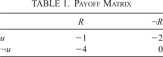
Imagine Alice’s payoff matrix is as given in table 1, which shows how much utility Alice gets, depending on whether she brings an umbrella when it rains or does not rain. By a simple calculation of Alice’s expected utility, we can determine how high her credence x in R must be before she decides to bring an umbrella.

(1)$\begin{array}{}\begin{array}{ccc}\mathrm{EU}\left(u\right)& =& x\left(\mathrm{-1}\right)+(1-x)\left(\mathrm{-2}\right)\\ & =& x-2\mathrm{.}\end{array}\end{array}$

(2)$\begin{array}{}\begin{array}{ccc}\mathrm{EU}(\neg u)& =& x\left(\mathrm{-4}\right)+(1-x)\left(0\right)\\ & =& \mathrm{-4}x\mathrm{.}\end{array}\end{array}$

We then have (1) > (2) if and only if $x>2/5$. So, Alice will bring an umbrella if $x>2/5$ and not bring an umbrella if $x<2/5$. For ease, we will conventionally decide that Alice will bring the umbrella if and only if $x>2/5$. All that matters for how much utility Alice ends up getting is (i) whether R and (ii) whether her credence is greater than 2/5.

Table 1.

Payoff Matrix

	R	¬R
u	−1	−2
¬u	−4	0

3.2. Reformulation

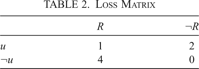
We need to reformulate this problem to suit our aims of constructing proper scoring rules. Since scoring rules are loss functions, we will describe Alice as an expected loss minimizer instead of as an expected utility maximizer. This choice is purely conventional. Table 2 reexpresses table 1 in terms of losses instead of gains.

Table 2.

Loss Matrix

	R	¬R
u	1	2
¬u	4	0

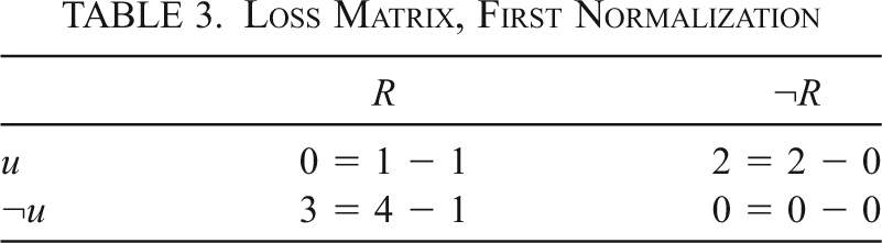
Notice that if it rains, Alice is sure to incur a loss of at least 1 no matter what she does. As far as her decision is concerned, this loss is irrelevant since it is merely a result of the state of the world. So, we can normalize table 2 by subtracting the minimum loss that is sure to result at each state. We then arrive at table 3.

Table 3.

Loss Matrix, First Normalization

	R	¬R
u	0 = 1 − 1	2 = 2 − 0
¬u	3 = 4 − 1	0 = 0 − 0

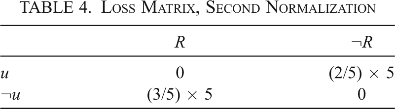
Finally, we rewrite table 3 as table 4 by dividing the loss in each cell by the sum of the total losses in each cell. In this case, the sum is 5, since Alice will lose 2 if she performs u and ¬R and will lose 3 if she performs ¬u and R.

Table 4.

Loss Matrix, Second Normalization

	R	¬R
u	0	(2/5) × 5
¬u	(3/5) × 5	0

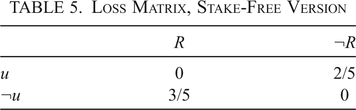
When considering this problem in isolation, we can forget about the sum of the losses. It represents the “stakes” of the problem, but it will not affect Alice’s decision. So, for now, we can rewrite the payoff matrix as table 5, which captures this single decision problem conspicuously. As before, all that matters for much (dis)utility Alice ends up getting is (i) whether R and (ii) whether her credence is greater than 2/5.

Table 5.

Loss Matrix, Stake-Free Version

	R	¬R
u	0	2/5
¬u	3/5	0

3.3. Scoring Rules and the Problem of the Umbrella

We can now design a scoring rule that will track how much of a loss (under our normalization) a credence of x in R will bring Alice. That is, given that her credence is currently x, we determine how much she expects to lose from her bet on rain.

First, let us determine how much she would lose if R and if ¬R, respectively. Per table 5, If R and $x\le 2/5$, Alice will lose 3/5, since she will not bring an umbrella. If $x\ge 2/5$ and ¬R, she will lose 2/5, since she will bring an umbrella. Otherwise she loses nothing.

Consider $G=(g_1,g_0)$, where

$g_1\left(x\right)=\{\begin{array}{cc}3/5& \text{if}x\le 2/5\\ 0& \text{if}x>2/5,\end{array}$

and

$g_0\left(x\right)=\{\begin{array}{cc}0& \text{if}x\le 2/5\\ 2/5& \text{if}x>2/5\mathrm{.}\end{array}$

Given Alice’s credence and R’s truth-value, G returns the amount Alice will lose.

Now suppose Alice wishes to evaluate a credence of y given her credence x. That is, she wants to determine how much she would expect to lose if she had decided whether to bring an umbrella on the basis of a credence of y in R.

We then have

$\begin{array}{ccc}{E}_x\left(G\right(y\left)\right)& =& x\times g_1\left(y\right)+(1-x)g_0\left(y\right),\\ & =& \{\begin{array}{cc}x\times 3/5& \text{if}y\le 2/5\\ (1-x)\times 2/5& \text{if}y>2/5,\end{array}\end{array}$

where E_x(G(y)) is minimized exactly when

$x,y\le 2/5$

or

$x,y>2/5\mathrm{.}$

So, G is a merely proper scoring rule.

3.4. The General Case

More schematically, we can represent the agent as choosing between two options, d ₁ and d ₀, where d ₁ is better to perform if P and d ₀ is better to perform if ¬P. That is,

$\begin{array}{c}L(d_1,P)\le L(d_0,P)\\ L(d_1,\neg P)\ge L(d_0,\neg P)\mathrm{.}\end{array}$

We again normalize losses in the same way we did in table 3 by setting

$L(d_1,P)=L(d_0,\neg P)=0.$

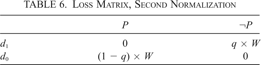
Then, in accord with table 4, we can now construct a loss matrix as expressed in table 6, where $q\in \left[0,1\right]$ and $W\in \left(0,\infty \right]$. Alice’s cutoff for performing d ₁ is represented by q. That is, if and only if Alice’s credence in $P<q$ will she perform d ₁. Otherwise, she will perform d ₀. The weight or stakes of the problem is represented by W. Again, we ignore W for now and focus only on the cutoff points for deciding whether to d ₁.

For any particular q, Alice sees no difference in expected value between two forecasts on the same side of q since those forecasts will lead to the exact same action.

Table 6.

Loss Matrix, Second Normalization

	P	¬P
d 1	0	q × W
d 0	(1 − q) × W	0

In this more general case, we can determine Alice’s valuation of a credence x with the merely proper scoring rule $G=(g_1,g_0)$:

$g_1\left(x\right)=\{\begin{array}{cc}1-q& \text{if}x\le q\\ 0& \text{if}x>q,\end{array}$

and

$g_0\left(x\right)=\{\begin{array}{cc}0& \text{if}x\le q\\ q& \text{if}x>q\mathrm{.}\end{array}$

3.5. Uncertainty about the Bet

We are often uncertain what bets we are actually going to face in the future. Supposing you are going to bet on P, you may still be uncertain whether you will face a q- or q′-problem. For instance, Alice may know she will be offered some bet that will return $1 if it rains, and $0 otherwise, but not yet know what price the bookie will offer her.

We will handle the more general case in a moment, but for now assume that there is some finite set $Q\subset [0,1]$ such that Alice has credence 1 that she will face some q-problem, where $q\in Q$. We will treat Q as a random variable representing the q-value of the decision problem Alice faces and use Pr(q ₀) as an abbreviation for $\mathrm{Pr}(Q=q_0)$.

So, if Alice is uncertain about the value of Q, what expected loss does she assign her credence x in P? Ignoring the stakes, we find

(3)$\begin{array}{}{h}_1\left(x\right):=\mathrm{EL}\left(x\right|P)=\sum _{\begin{array}{c}q\in Q\\ x\le q\end{array}}(1-q)\times \mathrm{Pr}\left(q\right)\mathrm{,}\end{array}$

(4)$\begin{array}{}{h}_0\left(x\right):=\mathrm{EL}\left(x\right|\neg P)=\sum _{\begin{array}{c}q\in Q\\ q<x\end{array}}q\times \mathrm{Pr}\left(q\right),\end{array}$

where h ₁ represents Alice’s expected loss of having credence x conditional on P, and h ₀ represents Alice’s expected loss of having credence x conditional on ¬P. That is, h_i represents Alice’s expected loss given the truth-value of P but with the q-value of the bet still undetermined.

We calculated h ₁ as follows: if P is the case and Alice’s credence x turns out to be less than or equal to Q, she will lose 1 − Q. If her credence turns out to be greater than Q, she will not lose anything. So, h ₁ just is the sum of 1 − q discounted by Alice’s credence $\mathrm{Pr}(Q=q)$ for every $q\ge x$. The formula for h ₀ is determined similarly.

We can then determine Alice’s unconditional expected loss of credence x in P by

${\mathrm{EL}}_x\left(x\right)=x\times h_1\left(x\right)+(1-x)h_0\left(x\right),$

where EL_x(x) is the loss Alice currently expects to suffer from her credence of x before she learns whether P is true or false. More generally, we can calculate Alice’s unconditional expected loss of alternative forecast y in P by

${\mathrm{EL}}_x\left(y\right)=x\times h_1\left(y\right)+(1-x)h_0\left(y\right),$

where EL_x(y) is the expected loss Alice assigns to using another forecast instead of her own, but with her utility function held fixed. It is easy to check that $H=(h_1,h_0)$ is in fact a merely proper scoring rule.

3.6. Letting the Stakes Count

As we noticed, two q-problems can have very different stakes. The same hand in blackjack matters a lot more at the $1,000 table than the $1 table, even though the probabilities remain the same.

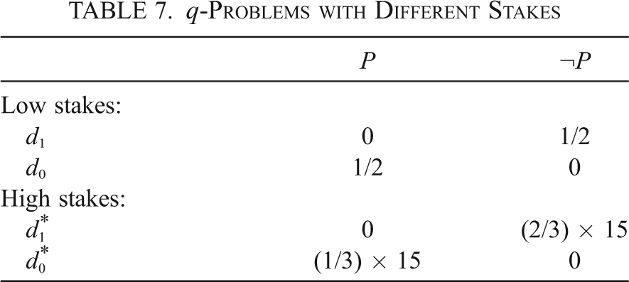
Furthermore, an agent may expect that if she faces a q-problem it will present her with stakes different from a q′-problem. Suppose, for instance, she is 50% confident she will face the low-stakes problem in the top panel of table 7 and 50% confident she will face the high-stakes problem in the bottom panel of table 7. Because the latter problem has much higher stakes, having her credence on the right side of 2/3 is significantly more important than having her credence on the right side of 1/2. In general, for any given q, the expected value of the stakes W can vary.

Table 7.

q-Problems with Different Stakes

	P	¬P
Low stakes:
d 1	0	1/2
d 0	1/2	0
High stakes:
$d_1^{*}$	0	(2/3) × 15
$d_0^{*}$	(1/3) × 15	0

Let E(W|q) be the expected value of W given that Alice faces a q-problem. Letting g ₁ represent the expected loss of credence x conditional on P and g ₀ be the expected loss of credence x conditional on ¬P, we have

(5)$\begin{array}{}{g}_1\left(x\right)=\sum _{\begin{array}{c}q\in Q\\ x\le q\end{array}}(1-q)\times E\left(W\right|q)\times \mathrm{Pr}(q),\end{array}$

(6)$\begin{array}{}{g}_0\left(x\right)=\sum _{\begin{array}{c}q\in Q\\ q<x\end{array}}q\times E\left(W\right|q)\times \mathrm{Pr}(q)\mathrm{.}\end{array}$

The overall expected loss Alice assigns forecast y if her credence is x is then

(7)$\begin{array}{}{\mathrm{EL}}_x\left(y\right)=x\times g_1\left(y\right)+(1-x)\times g_0\left(y\right)\mathrm{.}\end{array}$

Again, G is a merely proper scoring rule. Let $Q=\left\{q_1,\dots ,q_n\right\}$. If Alice’s credence is x where $q_i<x\le q_{i+1}$, then she assigns any y in the same interval the same expected loss she assigns herself. Otherwise, she assigns y a greater expected loss.

To determine G, what matters then is both how high the stakes are expected to be given that a q-problem is faced and how likely Alice thinks it is that she will face a q-problem. That is, what matters is the quantity

$M\left(q\right):=E\left(W\right|q)\times \mathrm{Pr}(q)\mathrm{.}$

We can then reformulate equations (5) and (6) above as

(8)$\begin{array}{}{g}_1\left(x\right)=\sum _{\begin{array}{c}q\in Q\\ x\le q\end{array}}(1-q)\times M\left(q\right),\end{array}$

(9)$\begin{array}{}{g}_0\left(x\right)=\sum _{\begin{array}{c}q\in Q\\ q<x\end{array}}q\times M\left(q\right)\mathrm{,}\end{array}$

where M(q) measures how important Alice thinks q-problems are to get right. Note that (i) $M\left(q\right)\ge 0$ and (ii) $M\left(q\right)=0$ if and only if $\mathrm{Pr}\left(q\right)=0$. Neither of these facts is surprising: it is never good to get a q-problem wrong, and if you think you might face a q-problem, then getting it right matters at least a little bit.

3.7. The Continuous Case

So far, we have assumed that q is in some finite set $Q\subset [0,1]$ to keep things discrete. However, Alice could potentially face a q-problem for any $q\in \left[0,1\right]$. The main difficulty is that once we make this generalization, the probability of any particular q-problem is 0.Footnote ¹⁸

The natural way to handle this problem is to trade out M(q) for a function m(q) that measures the probability density of facing a q-bet factored by the expected stakes of that bet. That is,

$m\left(q\right):=p\left(q\right)E\left(W\right|q),$

where p(q) is the probability density Alice assigns to the claim that she will face a q-problem. We call such an m Alice’s support function. The support function measures how much relative importance is assigned to each possible value of Q.Footnote ¹⁹

To get a handle on m, note that (i) $m\left(q\right)\ge 0$ and (ii) m is constantly 0 over some region [α, β] just in case Alice is certain that she will not face a q-problem for any $q\in \left[\alpha ,\beta \right]$. As with M, the first condition reflects the fact that it is never good to get a q-problem wrong. The second condition means that if Alice thinks it is possible she will face a q-problem for q in some region, then getting such a problem right matters at least a little bit.

By switching out M for m and the sums for integrals in equations (8) and (9), we can generate scoring rules when $Q=[0,1]$. With some reformulation and loss of generality, Schervish’s theorem is then:

Theorem 1 (Schervish). Let m(q) be a support function, and let

$\begin{array}{cc}{g}_1\left(x\right)& ={\int }_x^1(1-q)m\left(q\right)dq,\\ g_0\left(x\right)& ={\int }_0^{x}q\times m\left(q\right)dq.\end{array}$

Then $G=(g_1,g_0)$ is a proper scoring rule. If m is strictly positive almost everywhere, then G is a strictly proper scoring rule.

With some generalization, this method gets us every proper and strictly proper scoring rule, aside from uninteresting ones that, for example, assign every region infinite importance.

Note that the condition that m be positive almost everywhere is a kind of regularity condition. Alice will set $m\left(q\right)=0$ if and only if she is certain she will not face a q-problem for that q-value. So, if she leaves open the possibility (however remote) of facing any q-problem whatever, then she will use a strictly proper scoring rule to evaluate her credence.

3.8. Examples

Above, we defined the local versions of the Brier Score, Log Score, and Spherical Score. Let us see how these each encodes very different expectations about the bets Alice may face.

If Alice assigns constant weight to every point, we have

$m\left(q\right)=c,$

which generates the Brier Score (times c/2).

If Alice cares about points in [0,1] closer to 0 or 1 more than she cares about other points, she might set

$m\left(q\right)=\frac{1}{q\times (1-q)},$

which generates the Log Score.

If Alice weights points near .5 more than she weights other points, she may set

$m\left(q\right)=\frac{1}{{(2q^2-2q+1)}^{3/2}},$

which generates the Spherical Score.

Figure 1 provides a visual representation of each of these scoring rules along with their corresponding support functions.

Figure 1.

Brier, log, and spherical scores along with their support functions. Left, ascending curves represent g ₀(x) and descending curves represent g ₁(x) for the respective scoring rules.

The Brier Score is the most egalitarian of all scoring rules in terms of the decisions the user expects to make. Imagine you knew you were going to be offered a bet on X that paid $2 if X and $0 otherwise. The price of the bet will be chosen at random (i.e., by the uniform distribution on [0,2]). In is case, the Brier Score is the right scoring rule. The stakes of the bet are constant; that is, $E\left(W\right|q)=2$ for all q. Furthermore, since the value of $Q$ follows a uniform distribution, $p\left(q\right)=1$ for all q. So, $m\left(q\right)=2$.

The Logarithmic Score is approximately right when, in expectation, bets will be concentrated near the end points of the unit interval and when the stakes are high near those points. The Spherical Rule is best when the success of your decisions will likely depend on correct unbiased binary classification, that is, guessing whether X or ¬X is true depending on whether your credence in X is greater or less than .5.

In real life, of course, our views over the bets we will face on propositions are a lot messier. Suppose I am wondering whether my house will burn down in the next year. I do not yet know exactly which bet I will face on that proposition, but in expectation a credence of .01 is very different from a credence of .0001. In the former case, I will likely pay quite a bit for an insurance policy. So, relatively close to 0, my loss function will behave a lot like the Log Rule. However, a credence of 10⁻⁶ and a credence of 10⁻⁷ in this same proposition are roughly equivalent as far as my real-world success is concerned. Despite the value of my house, if my credence is low enough that it will burn down, I am effectively morally certain that it will not burn down. I assign, at some point, negligible practical weight to the possibility that I will wrongly bet that it will remain in tact for the next year. So the Log Rule will not be a perfect fit.

Similarly, the Spherical Score is a good approximation of the right score for my credence in whether it will rain. Whether I make the right decision about bringing an umbrella, buying baseball tickets in advance, or canceling my picnic hinges on whether my credence is above or below (approximately) .5. I doubt any decision I make will depend on whether my credence is on the correct side of .05 or .95. At that point, I am effectively certain it will not (will) rain as far as my decision making goes. Therefore, the correct support function will place more weight on middling regions of the unit interval and less weight on extreme regions.

3.9. Global Scoring Rules

Let us now briefly turn our attention to scoring global credence functions. The idea is the same: the expected score of an entire credence function is the expected loss an agent would incur from using that credence function to make bets.

The score of an individual credence x in proposition X at a world is the expected loss. That is, the score measures the expected loss given the actual truth-value of X before it is known exactly which bet on X the agent will face. Likewise, when we score an entire credence function b at a world, we plug in the actual truth-values of the propositions in $ℱ$, but we do not yet plug in the actual bets the agent faces. Indeed, she may not face a bet on some propositions at all.

The easiest way to determine this global score is simply to identify it with the (normalized) sum of the local scores:

$G(b,w)=\alpha \times \sum _{X\in ℱ}{G}_X\left(b\right(X),w(X\left)\right)\mathrm{,}$

where α is positive, and G_X is the scoring rule used for proposition X. In general, as we have seen, the scoring rule for the individual propositions will vary heavily, depending on the expected bets the agent may face. Furthermore, because we are much more likely to face bets on some propositions than on others, and because the stakes of those bets will vary heavily, some propositions will count much more to b’s overall score at w. For instance, it is much more likely that we will face a bet on whether it will rain than on whether there are an odd number of grains of sand in the Sahara. So, G(b,w) will give extra weight to the former proposition.

For this to work (i.e., for us to be able to simply add up a bunch of local scores) we need a way of localizing bets. That is, given your entire credence function, we need a way to determine which single proposition your decision to perform act u or ¬u is a bet on. You might, for instance, want to bring an umbrella if your credence in rain is high enough. But you may also decide to bring an umbrella if your credence that it will snow is high. So, your decision is not really a bet on rain, nor is it a bet on snow, but instead it is a bet on (rain or snow).

To do so, the best method seems to be to partition the set of states of the world into those in which you would rather perform u and those in which you would rather perform ¬u. With your utility assignments fixed, the proposition u is taken to be a bet on the disjunction of all the states in which performing u is in expectation better than performing ¬u.Footnote ²⁰ In this way, Schervish’s method can be used to generate an additive scoring rule that represents the expected loss of an agent’s entire doxastic state.

4.1. Experiments

Suppose Alice is a scientist interested in whether X. She decides to spend some resources to perform an experiment that will provide her with new evidence. She cannot perform every potential experiment, so she will have to make some choices on the basis of the expected informational value of the results. How might she go about deciding?

Following Greaves and Wallace (Reference Greaves and Wallace2006), we call a partition $ℰ$ of Ω an experiment if the agent will learn some element of that partition is true. We say that an experiment $ℰ$ is performed once the agent learns which element of $ℰ$ in fact obtains.

For example, suppose Alice is wondering whether her favorite team will win tonight. She knows that if Jake is pitching, there is a .75 chance they will win. Otherwise there is a .25 chance. If she looks at the team’s website, she can find out who is pitching. So, in this case, there are four relevant states $\{W\wedge P,W\wedge \neg P,\neg W\wedge P,\neg W\wedge \neg P\}$, where W stands for the proposition that her team wins, and P stands for the proposition that Jake is pitching. She can perform the experiment $ℰ$ of finding out who is pitching and thereby partition Ω into $P=\{W\wedge P,\neg W\wedge P\}$ and $\neg P=\{W\wedge \neg P,\neg W\wedge \neg P\}$.

If Alice performs $ℰ$, she will learn either P or ¬P. So, Alice’s posterior credence in W, denoted $b_{ℰ}\left(W\right)$, will either be $b\left(W\right|P)=.75$ or $b\left(W\right|\neg P)=.25$, although she does not yet know which. Suppose Alice’s current credence in W is .5. How valuable is the experiment $ℰ$ to her in expectation?

Before performing $ℰ$, Alice assigns her credence an expected loss of $\mathrm{EG}\left(.5\right)=.5\left(g_1\right(.5)+g_0(.5\left)\right)$. If she learns P, she will either get a score of g ₁(.75) or g ₀(.75). So, her expected score given that she learns P is

$b\left(W\right|P\left)g_1\right(.75)+b(\neg W\left|P\right)g_0\left(.75\right)=.75g_1\left(.75\right)+.25g_0\left(.75\right).$

Likewise, her expected score given that she learns ¬P is $.25g_1\left(.25\right)+.75g_0\left(.25\right)$. Given the constraints we have established, she must also have a .5 credence in P. So, the expected score she currently assigns to her as-yet-unknown posterior credence after performing $ℰ$ is

(10)$\begin{array}{}\mathrm{EG}\left(b^{\epsilon }ℰ\right(W\left)\right)=.375\left(g_1\right(.75)+g_0(.25\left)\right)+.125\left(g_0\right(.75)+g_1(.25\left)\right)\mathrm{.}\end{array}$

Greaves and Wallace show that updating by conditionalization is the policy that minimizes expected loss for all proper scoring rules. So, (10) is less than or equal to Alice’s current score of EG(.5), and the inequality is strict if G is strictly proper.

From a practical point of view, this result follows from Good (Reference Good1967), who shows that in any decision context, free information never has negative value in expectation.Footnote ²¹ Indeed, we can quantify the expected value of performing $ℰ$ as the difference between Alice’s current expected loss and her expected posterior loss, that is, as $\mathrm{Val}\left(E\right)=\mathrm{EG}\left(.5\right)-\mathrm{EG}\left(b^E\right(W\left)\right)$. If we identify utility with dollars, Alice should pay up to $\$\mathrm{Val}\left(E\right)$ to learn the result of experiment $ℰ$.Footnote ²²

Note that the precise value of an experiment depends on which scoring rule Alice uses for the proposition under investigation. Suppose, for instance, that Alice had the option of performing either $ℰ$ or an alternative experiment $ℰ$′ that would reveal who won the game with 20% probability and would reveal no relevant information otherwise. That is, if Alice performs $ℰ$′ instead of $ℰ$, then there is a 20% chance she will learn either that W or that ¬W for sure and an 80% chance her credence in W will remain at .5. If Alice can only perform one of the two experiments, she will prefer to perform $ℰ$ if she uses the Brier Score, but she will prefer to perform $ℰ$′ if she uses the Log Score.Footnote ²³

Put slightly differently, the evidence an agent chooses to gather will depend on her scoring rule, which in turn depends on what sorts of decisions she expects she will make on the basis of her credence in the proposition in question. The decision of which evidence to collect is, what we might call, practico-epistemic. The evidence itself will determine her credal state, but her process of investigation is a practical one.

Finally, we observe that some experiments are absolutely preferable to others. That is, sometimes Alice will prefer to perform $ℰ$₁ to $ℰ$₂ regardless of her scoring rule. For instance, suppose Alice is interested in whether Bob or Carol will win the upcoming election. One polling company asks 5,000 people whom they plan to vote for. A second company asks only 50 (distinct) people. If we stipulate that each company uses a reasonable method of selecting participants, Alice will always prefer to learn the results of the first poll to the results of the second, although she would prefer to learn the results of both polls to the results of either one.

When performing $ℰ$₁ is preferable to performing $ℰ$₂ according to every strictly proper rule, $ℰ$₁ first-order stochastically dominates $ℰ$₂. That is, regardless of the kinds of bets Alice expects to make, she is in expectation better off if she performs $ℰ$₁.Footnote ²⁴

4.2. Evaluation of Agents

One special kind of experiment we often conduct is to ask other agents what their credence is in some proposition. Instead of going to her favorite team’s website, for instance, Alice might ask Bob how confident he is that the team won.

Ex ante, Alice does not know what Bob thinks. We can determine Alice’s assessment of the value of asking Bob for his credence the same way we determined the value of other experiments above. Let $B$ be the experiment of asking Bob. Then $\mathrm{Val}\left(B\right)=\mathrm{EG}\left(.5\right)-\mathrm{EG}\left(b^B\right(W\left)\right)$. That is, the value of asking Bob is the expected difference in inaccuracy (according to Alice’s scoring rule) of her own credence after asking Bob and her current credence.

Note that $\mathrm{EG}\left(b^B\right(W\left)\right)$ is not Alice’s assessment of Bob’s inaccuracy but is instead her assessment of what her own inaccuracy will be after talking to Bob. For instance, suppose Alice knows that Bob always has credence 0 in truths and credence 1 in falsehoods. If Bob tells her he is certain that her team lost, then she will become certain that they won and vice versa. So, she is ex ante certain that Bob will be perfectly inaccurate and also certain that she herself will be perfectly accurate after talking to him.

More formally, we can capture this distinction between Alice’s assessment of her own expected posterior inaccuracy and her assessment of Bob’s expected inaccuracy as follows. Let $B=x$ refer to the proposition that Bob’s credence in W is x, and let $b_x\left(W\right):=b\left(W\right|B=x)$. We then haveFootnote ²⁵

(11)$\begin{array}{}\mathrm{EG}\left(b^B\right(W\left)\right)=\sum _{x}b(B=x)\left[b_x\left(W\right)g_1\left(b_x\right(W\left)\right)+(1-b_x(W\left)\right)g_0\left(b_x\right(W\left)\right)\right],\end{array}$

(12)$\begin{array}{}\mathrm{EG}\left(B\right)=\sum _{x}b(B=x)\left(b_x\right(W\left)g_1\right(x)+(1-b_x\left(W\right)\left)g_0\right(x\left)\right)\mathrm{.}\end{array}$

As before, then, the value of the experiment of asking Bob (i.e., eq. [11]) is determined by what Alice expects of the disutility of her own future credence, which of course depends on her expectations about what she will use her credence for. That is why we here look at G(b_x(W))—that is, the inaccuracy of Alice’s credences after talking to Bob.

Equation (12) measures Alice’s assessment of Bob’s inaccuracy before she learns what he actually thinks. Practically, her view of Bob’s inaccuracy measures how much Alice expects to lose if she were to switch over from her own credences to Bob’s to make decisions while retaining her preferences over outcomes. So, if she expects that Bob is more accurate than she is, she would prefer (ex ante) to use his credences to hers.Footnote ²⁶ Note that, if Bob is an epistemic expert for Alice, then equations (11) and (12) coincide. That is, if for any x, $b\left(W\right|B=x)=x$, then $g_i\left(b_x\right(W\left)\right)=g_i\left(x\right)$.

As with experiments, which agents are expected to be more accurate than which others is scoring-rule dependent. For instance, Alice might expect Bob to be more accurate with respect to the Brier Score but less accurate with respect to the Log Score than Carol is.Footnote ²⁷ If Alice uses the Brier Score, then she would prefer Bob’s credences to her own, given the decisions she actually expects to make.

Alice may also sometimes expect one agent to be more accurate than another regardless of which scoring rule she uses. For example, suppose Alice treats Bob and Carol both as epistemic experts, but she knows that Carol will have either credence .8 or .2 in W, while Bob will have either credence .6 or .4 in W. It is easy to check, by equation (12), that for any G that is strictly proper, Carol is in expectation more accurate than Bob. So, regardless of the bets Alice expects she will make, she thinks she would be better off using Carol’s credences than Bob’s credences.Footnote ²⁸ In other words, one agent is judged absolutely more accurate than another if she is thought to be doing better regardless of the purposes of inquiry. One agent is judged better relative to a particular rule if she is thought to be doing better relative to the particular purposes of inquiry for the proposition(s) in question.