I. Introduction
Numerous empirical studies estimate demand functions for alcohol beverages. In many studies, the focus is price sensitivity, but income elasticities also are important, especially for wine and distilled spirits. Price elasticity estimates are utilized for taxation and pricing policies, while income estimates can be used for anticipation of demand growth arising from differences in real incomes over time or across countries. Also important are tests of basic theoretical constructs and application of new econometric techniques or new data. Increasingly, price estimates are a source of debate over public policies that address alcohol-related problems and harms (Babor et al., Reference Babor, Caetano and Casswell2010; Cawley and Ruhm, Reference Cawley, Ruhm, Culyer and Newhouse2011; Cook, Reference Cook2007). As a result of research efforts over the past 50 years, demand elasticities for alcohol are widely available for developed countries, especially English-speaking and Scandinavian countries. The empirical estimates for price and income analyzed here cover 21 different countries for wine and spirits.Footnote 1
Given the multiplicity of studies and estimates, several different summaries of demand elasticities are available. First, as a prelude to econometric estimation, many empirical studies include a selective summary of prior elasticity estimates. Examples include Collis et al. (Reference Collis, Grayson and Johal2010), Eakins and Gallagher (2005), Lariviere et al. (Reference Lariviere, Larue and Chalfant2000), Pompelli and Heien (Reference Pompelli and Heien1991), and Tremblay and Tremblay (Reference Tremblay and Tremblay2005). Second, traditional narrative surveys provide more detailed descriptions of individual studies along with a summary of estimates, usually in tabular form. Examples of well-known narrative surveys are Chaloupka (Reference Chaloupka, Bonnie and O'Connell2004), Edwards et al. (Reference Edwards, Anderson and Babor1994), Leung and Phelps (Reference Leung, Phelps, Hilton and Bloss1993), and Ornstein and Levy (Reference Ornstein, Levy and Galanter1983). Third, meta-analyses provide statistical summaries of empirical estimates in the form of averages, weighted averages, and meta-regressions that use estimated elasticities as dependent variables. Recent examples are Fogarty (Reference Fogarty2009), Gallet (Reference Gallet2007), and Wagenaar et al. (Reference Wagenaar, Salois and Komro2009). As discussed below, these analyses contain several shortcomings, including insufficient attention to outliers and publication bias. However, compared to narrative reviews, meta-analysis has several advantages as a method for summarizing and synthesizing an empirical literature (Borenstein et al., Reference Borenstein, Hedges, Higgins and Rothstein2009; Nelson and Kennedy, Reference Nelson and Kennedy2009; Stanley and Doucouliagos, Reference Stanley and Doucouliagos2012). Meta-analysis can produce a synthesis that is more transparent and less subject to reviewer biases, which may be hidden or not obvious in narrative reviews. Weights used in meta-analysis are derived from statistical theory, rather than determined by each individual reviewer. Meta-analysis also is more appropriate as a literature grows in size, because focused narratives are harder to conduct and are subject to Type II errors (Florax, Reference Florax, Florax, Nijkamp and Willis2002; Hedges and Olkin, Reference Hedges and Olkin1985). Further, aside from simple averages, narrative reviews lack a well-defined method for integrating relationships or producing summaries that contribute to an understanding of quantitative differences among primary studies. Using meta-regression analysis, a more detailed synthesis is possible. Lastly, meta-analysis is especially suited to empirical estimates that share a common unit of measurement and underlying theory, such as unit-free price and income elasticities of demand obtained from recorded alcohol consumption data.
The objective of this paper is to summarize and synthesize estimates of price and income elasticities for wine and distilled spirits, while accounting for possible influences of outliers and publication bias. Prior meta-analyses largely ignored these data issues, and estimates reported here should be more robust. As is well known, outliers or influential data points can result in statistical estimates that perform poorly (Kennedy, Reference Kennedy2008). It is important to recognize that outliers in a meta-analysis are multidimensional because both estimates of elasticities and their standard errors (or precision) are required for analysis. For wine prices, the initial sample contains 197 estimates drawn from 104 primary studies. However, detailed analysis is carried out using a 10% trimmed sample of 178 observations. For wine income elasticities, the initial sample contains 172 estimates and the trimmed sample has 155 observations. Similar restrictions are placed on price and income elasticities for spirits, where the initial samples have 202 and 179 observations drawn from 111 primary studies. Trimmed samples contain 182 and 160 observations, respectively. The samples also are designed to reduce chances of statistical dependence among estimates by restricting the number of estimates per study.
The second issue addressed is publication bias due to selectivity. Publication bias has been defined in different ways and has several dimensions, but it generally means that published estimates have been selected in some manner, typically based on sign and significance of findings (Song et al., Reference Song, Eastwood and Gilbody2000; Stanley and Doucouliagos, Reference Stanley and Doucouliagos2012). Selectivity associated with the editorial, review, and dissemination processes also play a role. If published estimates are a biased sample of all possible estimates, results of a literature review will be biased and potentially misleading. This bias applies to narrative reviews and meta-analyses (Rothstein et al., Reference Rothstein, Sutton, Borenstein, Rothstein, Sutton and Borenstein2005). However, it is possible to test statistically for publication bias, measure its extent or severity, and correct summary estimates for bias. Until recently, tests for publication bias in economics were infrequent, but early examples include Ashenfelter et al. (Reference Ashenfelter, Harmon and Oosterbeek1999), Card and Krueger (Reference Card and Krueger1995), and Smith and Huang (Reference Smith and Huang1995). As interest in meta-analysis has expanded, these tests are more common and are now viewed as a standard part of an analysis (Nelson, Reference Nelson2011, Reference Nelson, Johnston, Rolfe and Rosenberger2013a; Roberts and Stanley, Reference Roberts and Stanley2005; Stanley and Doucouliagos, Reference Stanley and Doucouliagos2012). This paper is the first attempt to correct for publication bias for wine and spirits demand elasticities.
The remainder of the paper is divided into four sections. Section 2 describes the basic steps in the analysis, including selection of primary studies and estimates. Weighted-average estimates for elasticities are reported, where weights are based on inverse variances of effect sizes. Both fixed-effect and random-effects means are reported for full and trimmed samples. Country-specific averages also are reported. Section 3 contains an investigation of publication bias using several methods, including funnel graphs, funnel-asymmetry tests, and cumulative meta-analysis. Weighted-averages corrected for publication bias are reported. Section 4 examines effects of heterogeneity on primary estimates and presents metaregressions that correct for factual and methodological dispersion, publication bias, dependence, and heteroskedasticity. Section 5 contains a summary of results and discusses implications for alcohol taxation, minimum pricing, and other control policies. Overall, the demands for wine and spirits are less price elastic than reported in prior summaries and meta-analyses. Using cumulative meta-analysis, the average price elasticity is about −0.45 for wine and −0.55 for spirits. Income elasticities are about 1.00 for both beverages. However, significant country-level differences also are demonstrated.
II. Meta-Analysis: Procedures and Weighted Averages
A. Selection of Primary Studies and Estimates
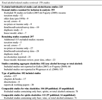
The starting point for a systematic review is a search of the literature on alcohol demand, including the “gray” literature such as unpublished working papers. A literature search was conducted by the author during the months of August–September 2012, with recent meta-analyses providing a useful starting point. Articles, chapters, books, reports, dissertations, and working papers were examined on alcohol demand and alcohol-related outcomes, such as traffic fatalities, crime, labor productivity and wages, and youth consumption. Some econometric studies on alcohol harms include first-stage or structural demand estimates, which are easily overlooked. Search terms used were combinations of “alcohol” AND “demand” (OR “price” OR “elasticity” OR “tax”). Complementary searches also were conducted using “beer,” “wine,” “liquor,” and “distilled spirits.” Databases searched included AgEcon Search, EconLit, JSTOR, RePEc, and SSRN and online retrieval engines for EBSCO Host, ProQuest, ScienceDirect Journals, and Wiley Online Library. Numerous Google searches also were conducted, which were helpful in retrieving working papers and other unpublished materials. References in the studies were used for ancestral-based retrievals. The search was restricted to materials in the English language but not limited to articles in peer-reviewed journals. Table 1 summarizes search and selection processes, where a total of 578 primary studies were recovered and examined. Hard copies were obtained for each of these studies in their entirety. Abstracts, tables, and other summaries were screened by the author to select alcohol demand studies that provide comparable estimates for price and income elasticities of alcohol beverages. There are 182 studies that provide elasticity estimates, which cover beer, wine, spirits, and total alcohol. There are 64 studies that were not included in Fogarty (Reference Fogarty2009) or Gallet (Reference Gallet2007), and 58 studies included in their analyses that are excluded here. The present analysis is based on estimates obtained from 104 studies for wine elasticities and 111 studies for distilled spirits. A complete listing of the retrieved estimates (effect sizes and standard errors) is available upon request from the author.
Summary of Literature Search: 578 Alcohol Studies

Note: A complete bibliography listing of the 578 studies and tables with the extracted data for this study are available upon request or at http://econ.la.psu.edu/people/biographies/nelson_bio.shtml.
As summarized in Table 1, primary studies and estimates included in the present analysis reflect several exclusion criteria, which help ensure comparability or quality of estimates. Alcohol price and tax elasticities are not comparable unless the tax elasticity is transformed (Cook, Reference Cook2007, p. 72), meaning alcohol tax elasticities are excluded here. It is unclear how previous meta-analyses handled this problem. Also excluded are estimates based on individual-level survey data (youth and young adult studies), where alcohol consumption is self-reported, prices are imputed, and elasticities cover a range of behaviors (drink participation, frequency, amount, binging, etc.). Household survey studies are included if they provide aggregate elasticity estimates. Studies are excluded that use firm-level data, brand data, and narrow beverage categories (vodka, wine varietals). Primary studies based on predominantly older data (pre-1950) have been excluded. Because weighting of elasticities is a standard procedure in meta-analysis, studies are excluded where variance data are missing or cannot be estimated (see below). Finally, as indicated in Table 1, 10–20% of studies were found in the gray literature. The purpose of these restrictions is to produce more uniform samples that avoid the criticism that a quantitative synthesis is combining “apples and oranges.” However, factual and methodological heterogeneity are certain to exist in primary studies and estimates, which is the focus of the metaregression analysis.
B. Data Coding and Potential Moderator Variables
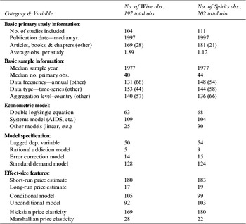
Data on each study were collected and recorded by the author, including page or table numbers for the primary estimates. No elasticity values were estimated, which is a reason for excluding most linear model estimates. Following previous meta-analyses, data also were collected on a variety of potential moderator variables, which are summarized in Table 2. In general, moderator variables are conditioned so there are sufficient positive observations in each of several possible categories. No attempt was made to collect data on every possible estimation method or model (2SLS, 3SLS, MLE, SUR, etc.) as some econometric methods are employed infrequently by only a few studies. For example, only five estimates for wine are based on a rational addiction model. Metaregressions should properly pool these observations with similar categorical variables. A variable for substitute beverage prices is excluded because it is always included in multiequation system models and rarely in single equation models. Metaregressions reported below estimate parsimonious models that concentrate on fewer, more broadly defined moderator variables and avoids the collinearity inherent in numerous methodological variables.
Summary of Primary Study Descriptors

Notes: The summary is based on the full sample for price elasticities. Numbers in parentheses are counts in the “other” categories.
C. Addressing Dependence and Precision
Empirical studies in economics frequently report multiple estimates based on the same data or major portions of the same data set. Using all estimates creates within-study dependence or correlation, which will bias summary statistics. More weight is assigned to primary studies with multiple estimates than to studies with one or two estimates. Equally important, using multiple estimates will bias standard errors of summary statistics, with understatement of errors being the generally expected outcome (Borenstein et al., Reference Borenstein, Hedges, Higgins and Rothstein2009, p. 226). Dependence problems have several possible solutions , including use of a single “best” estimate per study, hierarchical/multilevel models, and cluster robust standard errors (Nelson, Reference Nelson, Johnston, Rolfe and Rosenberger2013a). Between-study dependence also occurs when primary investigators use the same data to estimate different models in separate publications or different investigators use the same data or very similar data. Following Fogarty (Reference Fogarty2009, p. 437), collection of effect sizes was restricted to one or two estimates per primary study or model. In general, the primary author's preferred result was selected from each study, and an important variation was used to capture different model specifications or estimation methods. While this restriction reduces within-study dependence, it does not fully address between-study dependence. In particular, several authors have published multiple studies using similar data sets, such as country-level models using annual time-series data (e.g., Duffy, Reference Duffy1990, Reference Duffy1991, Reference Duffy1995; Selvanathan and Selvanathan, Reference Selvanathan and Selvanathan2005, Reference Selvanathan and Selvanathan2006, Reference Selvanathan and Selvanathan2007). These authors tend to use different econometric methods, resulting in different “treatment effects.” Because the policy implications are potentially important, metaregressions reported below include cluster robust standard errors for seven different country groupings, which address data dependencies at this aggregate level.
Standard meta-analysis methods require estimates of precision for effect sizes in the form of standard errors (Stanley and Doucouliagos, Reference Stanley and Doucouliagos2012, p. 27). For about half the effect sizes, standard errors could be obtained directly, for example, the primary study reports a price elasticity estimate and its standard error (or t-statistic or p-value). For the other half, standard errors had to be obtained from other estimates reported in the study, for example, the primary study reports a regression coefficient for price and its standard error or t-statistic. The reported elasticity is typically a derived estimate. This information was used to derive a standard error for the reported elasticity. Thus, if an investigator reports a price coefficient and t-statistic, a standard error for the price elasticity was estimated by dividing the elasticity value by the t-statistic on price. A similar procedure was used by Fogarty (Reference Fogarty2009). This procedure introduces bias in standard errors, with expectation of an upward bias as covariance terms are ignored. As a check on this procedure, averages for standard errors can be compared by collection method. For wine price elasticities, mean standard errors (se) are 0.216 (se=.138) and 0.234 (.183) for self-reported and estimated errors, respectively. For wine income, means are 0.273 (.171) and 0.380 (.333). For spirits price elasticities, means are 0.229 (.326) and 0.280 (.266). For spirits income, means are 0.234 (.177) and 0.320 (.245). A slight upward bias is suggested for price elasticities. Mean errors for income are larger, although confidence intervals also are wider. A possible implication of these results is underweighting of elasticities with estimated standard errors, which is examined further below.
D. Weighted-Average Price and Income Elasticities
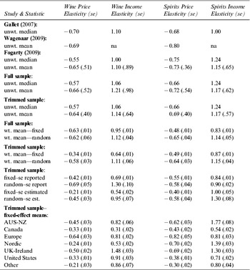
Weighted and unweighted averages are computed for full and trimmed samples, which are summarized in Table 3. Also presented are averages reported in Fogarty (Reference Fogarty2009), Gallet (Reference Gallet2007), and Wagenaar et al. (Reference Wagenaar, Salois and Komro2009). Across the studies, unweighted averages by beverage are approximately: wine price elasticity, −0.65; wine income, 1.10; spirits price, −0.70; and spirits income, 1.20. Despite differences in the samples employed, unweighted averages in several studies are broadly consistent with one another.
Average Wine and Distilled Spirits Elasticities

Notes: Weighted means for fixed and random effects computed using CMA 2.2 (Borenstein et al., Reference Borenstein, Hedges, Higgins and Rothstein2008). Standard errors reflect rounding. Trimmed sample sizes with reported (estimated) standard errors are: wine price, 85 (93); wine income, 68 (87); spirits price, 90 (92); and spirits income, 78 (82). Definitions for country groupings are reported in Section IV.
For samples used in the present study, weighted means are reported using fixed-effect and random-effects models. In a meta-analysis, the fixed-effect model uses inverse variances for weights and treats dispersion in estimates as due solely to stochastic sampling error in each primary study (Borenstein et al., Reference Borenstein, Hedges, Higgins and Rothstein2010). That is, all studies are viewed as estimating a common, or fixed, population effect size. Estimates with smaller standard errors provide more precise information about the population value and are given greater weight. The plural or random-effects model also accounts for variation in population values by estimating a common between-study variance based on the observed dispersion, which is added to study-level variances. Inverses of combined variances provide the weights for each effect size. Thus, in the random-effects model, true effect sizes are similar or comparable but not identical across studies. This is the simplest procedure for addressing heterogeneity in the estimates. Compared to fixed-effects, random-effect models assign greater weight to less precise studies and, as pointed out by Fogarty (Reference Fogarty2009, p. 455), the weights reduce the importance of outliers among standard errors.
Weighted means are reported for both full and trimmed samples. The purpose of trimming is to reduce the importance of outliers in both elasticities and standard errors, resulting in more robust summary estimates. This is a form of sensitivity analysis. As noted by Sutton et al. (Reference Sutton, Abrams and Jones2000, p. 148), when extracted data in a meta-analysis vary widely, “the effect of using a reasonable range of values … where uncertainty exists about the results should be explored through sensitivity analysis.” Trimmed samples are obtained by eliminating 10% of each sample by discarding 2.5% of the largest effect sizes, 2.5% of the smallest effect sizes, 2.5% of the largest standard errors, and 2.5% of the smallest standard errors. As indicated in Table 3, trimming the samples has no effect on unweighted medians and only a small effect on unweighted means. However, standard errors for unweighted means are reduced by about 25%–35%.
Using fixed-effect models and full samples, Table 3 indicates a wine price elasticity of −0.63 and an income elasticity of 0.95. Random-effects averages for wine price and income are about the same, −0.62 and 1.12. These estimates are smaller (less elastic) than unweighted elasticities. Using trimmed samples, fixed-effect wine elasticities are −0.34 for price and 0.64 for income, indicating that outliers are important. Different weighting used for random-effects yields values that change little after trimming, −0.58 and 1.11. Using fixed-effect models and full samples, spirits elasticities are −0.48 for price and 0.83 for income, which are smaller than unweighted values. Random-effects averages are −0.65 and 1.14. Trimmed means for spirits are about the same as full samples, although fixed- and random-effect values differ. The main effect of trimming is a reduction in standard errors for each mean. Results also show that weighted means depend on the model used. The next-to-last set of rows display results with two data restrictions: trimmed samples and reported (or estimated) standard errors. For wine, average price and income estimates with reported standard errors are larger (more elastic) than elasticities with estimated standard errors. For spirits, average price elasticities with reported standard errors are larger (more elastic), while income elasticities are smaller (less elastic). The differences again illustrate the importance of sensitivity analysis for samples and models. The last panel examines heterogeneity due to country of origin. Significant differences exist at the country level for both price and income. These differences are examined below and contrast with findings reported in Fogarty (Reference Fogarty2009, p. 428), particularly for spirits.
III. Publication Bias: Detection and Treatment
Publication bias occurs when primary researchers search among elasticity estimates and select those with statistically significant coefficients, “correct” signs, and larger, more elastic values.Footnote 2 The result is a biased set of estimates, with expectations of a positive association between effect sizes and their standard errors, that is, less precise estimates are more likely to be published if they have larger effects. The purpose of this section is to determine whether publication bias exists for the samples of wine and spirits elasticities, measure the extent of bias, and report average elasticities corrected for bias. A standard set of procedures is used. It should be noted, however, these procedures do not fully account for dispersion of the estimates. The next section incorporates observed heterogeneity into the model.
A. Funnel Graphs
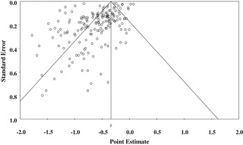
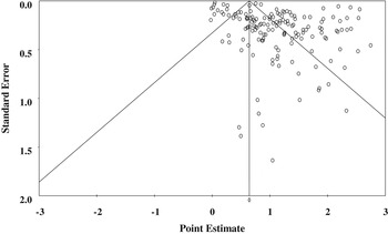
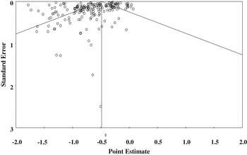
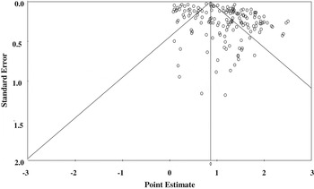
A standard method for detecting publication bias is the funnel graph. Briefly, the horizontal scale measures the effect size and the vertical scale measures the standard error (or precision). In the absence of publication bias, a plot of effects against their errors should be symmetric about the weighted mean. However, a “funnel-shaped” plot is expected due to heteroskedasticity as larger effects tend on average to have larger errors, regardless of publication bias. In the presence of bias, plots can be either less dense or asymmetric. First, suppose that the true effect in the population is zero. If studies with significant results are more likely to be published, bias is revealed in the plot as an empty area around zero, which results from nonpublication of insignificant or null results regardless of direction or sign. Second, suppose instead that the true effect is not zero but, rather, some small or moderate-size value. Bias will appear as an asymmetric plot as studies with small effects and large errors are less likely to be published or reported. Asymmetry also reveals the direction of bias as successful publication tends to be associated with both sign and significance of results. Funnel plots are an informal method, so it is important to recognize that a skewed plot also can result from underlying heterogeneity in the sample, such as basic differences in study design or primary data.
Figures 1 and 2 show funnel graphs for wine price and income elasticities. Vertical lines indicate fixed-effect means, reflecting a concern that random effects are due in part to publication bias (Stanley and Doucouliagos, Reference Stanley and Doucouliagos2012, p. 82). Diagonals indicate 95% confidence intervals for the means. Both graphs for wine indicate asymmetry in primary estimates, with a negative bias for price and a positive bias for income. Figures 3 and 4 show funnel graphs for spirits price and income elasticities. Asymmetries also are suggested for spirits, although perhaps not as strongly as for wine. More formal metaregression tests are required to confirm the existence of publication bias.
Funnel Plot—Wine Prices (mean=−0.34)

Funnel Plot—Wine Income (mean=0.64)

Funnel Plot—Spirits Prices (mean=−0.49)

Funnel Plot—Spirits Income (mean=0.87)

B. Metaregression Analysis of Publication Bias: FAT–PET Results
In the absence of publication bias, effect size estimates and their standard errors are independent. If not, they are correlated and summary statistics and standard errors are biased. For the i-th observation (i=1, … , N) , a regression-based test of this association can be represented as (Card and Kruger, Reference Card and Krueger1995; Stanley and Doucouliagos, Reference Stanley and Doucouliagos2012)
 $$ES_i = \beta _1 + \beta _0 Se_i + \varepsilon _i $$
where ES is the estimated price elasticity in study i, Se is its standard error, and ε is a stochastic error term. Absent selection and heterogeneity, observed effects should vary randomly about the true effect size, β 1, independent of standard errors. However, if model specifications are selected based on significance of the main covariates, effect sizes will vary directly with standard errors. Because estimates are inherently heteroskedastic, it is appropriate to divide equation (1) by the standard error to yield (Egger et al., Reference Egger, Davey-Smith, Schneider and Minder1997; Stanley, Reference Stanley2005)
 $$t_i = \beta _0 + \beta _1 (1/Se_i ) + \upsilon _i $$
where t i is the t-statistic for the i-th observation, 1/Se is its precision, and υ is an error term corrected for heteroskedasticity. Estimating equation (2) by ordinary least squares (OLS) is equivalent to estimating equation (1) by weighted least squares (WLS) with inverse variance weights. A test of H0: β 1=0 is a test for absence of publication bias or funnel-asymmetry test (FAT). If FAT rejects symmetry, the estimate of β 0 is interpreted as the mean effect size corrected for bias, referred to as the precision-effect test (PET).
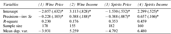
Table 4 shows results for FAT-PET regressions for price and income elasticities, estimated using trimmed samples. Applying FAT, all intercepts are statistically significant, and absolute values between 1.0 and 2.0 are consistent with substantial selection bias (Doucouliagos and Stanley, Reference Doucouliagos and Stanley2013). Applying PET, the coefficients indicate average price elasticities of −0.23 and −0.39 for wine and spirits, respectively. Income elasticities are 0.39 and 0.66. R-square values are somewhat low, suggesting that additional corrections for heterogeneity should be incorporated. Compared to previous analyses, Fogarty (Reference Fogarty2009, p. 458) reports moderate bias only for beer price elasticities. Funnel plots presented in Fogarty appear to indicate bias also for wine and spirits price elasticities. However, he reports that a regression-based test failed to detect bias for wine and spirits elasticities. Absent formal results from Fogarty's test, a more detailed comparison is not possible. Gallet (Reference Gallet2007) and Wagenaar et al. (Reference Wagenaar, Salois and Komro2009) did not test for bias. In any event, more powerful tests for publication bias are reported below.
Regression-Based Tests for Publication Bias
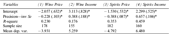
Notes: Dependent variable is t-statistic value for elasticity estimates. Standard errors in parentheses based on White's heteroskedastic robust OLS estimator. Asterisks indicate statistically significant at the 95% confidence level.
C. Cumulative Meta-Analysis: Weighed-Mean Elasticities by Precision Restrictions
An alternative to FAT-PET regressions is to order the data by precision and focus attention on more precisely estimated effect sizes (Borenstein et al., Reference Borenstein, Hedges, Higgins and Rothstein2009, p. 289; Stanley and Doucouliagos, Reference Stanley and Doucouliagos2012, p. 56). If the least precise estimates are biased, it is possible to think of assigning zero weight to these estimates relative to those with smaller errors, regardless of effect sizes (Stanley et al., Reference Stanley, Jarrell and Doucouliagos2010). With trimmed data ordered by precision, a cumulative meta-analysis is an analysis run with the first observation, then repeated with the first two observations, and so on until all observations are analyzed. What is arbitrary is the cutoff for selection of “more precise” estimates. Reported here are values at the medians (50th percentile by precision), which tends to focus on estimates with self-reported standard errors. In this framework, average elasticities obtained using cumulative meta-analysis and trimmed samples are:
Wine price, fixed and random effects: −0.32 (se=.01) and −0.46 (.04),
Wine income, fixed and random effects: 0.61 (.01) and 0.99 (.08)
Spirits price, fixed and random effects: −0.47 (.01) and −0.54 (.04),
Spirits income, fixed and random effects: 0.83 (.01) and 1.03 (.06)
Compared to random-effects means reported in Table 2 for trimmed samples, the average wine price elasticity is smaller by 20% (−0.46 compared to −0.58) and spirits price elasticity is smaller by 15% smaller (−0.54 compared to −0.64). Income elasticities are 10% smaller. Compared to estimates in Table 4, these are somewhat larger values.
In summary, publication selection bias is important for estimates of wine and spirits elasticities. A meta-analysis that corrects for publication bias yields average price and income elasticities that are less elastic, indicating upward bias in reported results. The magnitude of this effect is important both statistically and for interpretation and use of estimates. As a simple and direct method for reducing publication bias, cumulative meta-analysis is attractive as it permits a focus on higher quality estimates. The next section examines the extent to which heterogeneity, including country-level differences, matters for detection of publication bias and for synthesis of empirical estimates.
IV. Metaregression Analysis of Heterogeneity and Publication Bias
Metaregression is a fairly recent addition to the tool kit of applied researchers (Stanley, Reference Stanley2001). Surveys of meta-analysis in economics, such as Nelson and Kennedy (Reference Nelson and Kennedy2009), indicate that most analysts choose to focus on methodological differences in primary studies. However, these regressions are not necessarily the most useful for policymakers because they often reveal little about effects for different populations or cohorts, different time periods, different economic conditions, and so forth (Nelson, Reference Nelson, Johnston, Rolfe and Rosenberger2013a). For example, metaregressions in Fogarty (Reference Fogarty2009, p. 33) include 17 variables for econometric methods. In Gallet (Reference Gallet2007, p. 128), there are 31 variables for econometric methods. There also are five variables that describe primary populations in some studies (men, women, adults, young adults, teens), but observations are limited in several instances (Gallet, Reference Gallet2007, p. 124). Both studies pool observations, so common marginal effects are imposed for beer, wine, spirits, and total alcohol. Differences among beverages cannot be detected in this framework, which is a shortcoming for policy applications.
Although regressions in prior studies may be useful for empirical researchers, they lack a policy context. The objective in this section is different. For each beverage, covariates are included that measure methodological and factual dispersion, but the focus of the investigation is two effects: (1) significance of precision variables, which correct for publication bias; and (2) importance of country-level differences. If the precision variable is significant, this reinforces concerns noted above for publication bias. Neither previous metaregression analyses included a precision variable. If country-level differences are significant, this informs policymakers about persistent differences in empirical estimates. Gallet omitted country-level effects, and Fogarty reported only summary averages. Exclusion criteria described above preclude identification for demographic groups because most estimates are based on aggregate, population-level data.
Adding moderator variables to equation (1) yields a WLS metaregression model of heterogeneity and publication bias. Specifying all moderator variables as categorical binary dummies preserves interpretation of coefficients in equation (1), with the intercept as an estimate of the true effect size for the null category and the precision coefficient as an index of distortion due to publication bias. As a correction for heteroskedasticity, weights are based on inverse variances of elasticity estimates. A specific-to-general approach is used to arrive at a preferred model specification. Only core moderator variables are used in the initial specification, and then additional variables are added selectively for a sensitivity analysis. A metaregression that details differences by country is useful for policy purposes. The country groups are also used to obtain cluster robust standard errors. Seven country groupings are specified as follows:
Australia and New Zealand: wine (24 price observations, 21 income observations); spirits (21, 18); Canada: wine (32, 24); spirits (24, 21); Europe (Cyprus, Czech Republic, France, Italy, Poland, Romania, Spain): wine (12, 11); spirits (7, 8); Nordic (Denmark, Finland, Norway, Sweden): wine (26, 21); spirits (25, 23); United Kingdom and Ireland: wine (42, 42); spirits (45, 44); United States: wine (35, 29); spirits (53, 40); and Other (Chile, China, Japan, Russia): wine (7, 7); spirits (7, 6).
In addition to country-level dummies, covariate pairs included are: (1) two variables related to the theoretical model; (2) two variables related to the time period; (3) two variables describing data frequency and aggregation; and (4) two variables describing the econometric model. In primary studies, own-price estimates are based on either a compensated (Hicksian) or uncompensated (Marshallian) demand model, with expectation of a more elastic price elasticity in the latter case (Fogarty, Reference Fogarty2009). Hence, a negative sign is expected for a dummy variable for Marshallian estimates. The model also can be conditional on total alcohol expenditure or unconditional, with expectation of larger income elasticity in the former case. A positive sign is expected for a dummy variable for “conditional” estimates. Time variables are, first, midyear of the primary data and, second, year of publication of the primary study. No specific expectations are possible for coefficient signs, but it is often argued that publication date accounts for more advanced econometric methods used in recent studies. Two data variables account for the level of aggregation: annual vs. higher frequency data (quarterly, monthly); and time-series vs. non–time-series data (panel, survey). It is often argued that time-series data capture short-run behavior, and thus smaller elasticities are expected. Lastly, primary model specification can capture short-run or long-run behavior, where long-run estimates should be larger (more elastic). The model specification also can be either a single-equation or a demand system model, which captures possible differences due to “flexibility” of the model estimated (e.g., constant elasticity vs. derived estimate).
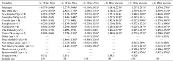
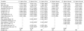
Results are presented for wine and spirits elasticities in Tables 5 and 6. Combinations of paired variables were estimated, but some results are not reported in the interest of conserving space. The precision variable is always statistically significant. Hence, publication bias is confirmed using a more powerful test. Dummies for estimated standard errors are significant in most reported regressions (negative for price and positive for income). At the suggestion of a referee, results are reported in regressions (3) and (6) for all country dummies using a model due to Suits (Reference Suits1984); see also Kennedy (Reference Kennedy1986). In this model, the sum of country dummies is constrained to add up to zero, so individual coefficients are deviations from the average. Country dummies and intercepts differ from regressions (2) and (5) by the magnitude of the coefficient for Other countries. This coefficient is reported explicitly rather than subsumed in the intercept.
Metaregressions for Wine Price and Income Elasticities

Notes: Cluster robust standard errors in parentheses; asterisks indicate statistical significance at the 95% level. Weighted least-squares regressions estimated with inverse variances for weights. Regressions (3) and (6) are estimated by constrained weighted least squares using Stata 12.
Metaregressions for Distilled Spirits Price and Income Elasticities

Notes: Cluster robust standard errors in parentheses; asterisks indicate statistical significance at the 95% level. Weighted least squares regressions estimated with inverse variances for weights. Regressions (3) and (6) are estimated by constrained weighted least-squares using Stata 12 (see text).
A. Metaregressions for Wine Elasticities
Table 5 reports WLS regressions for wine price and income elasticities. The precision variable is always significant, with absolute values between 2.0 and 3.0. These values are indicative of substantial publication bias. Dummies for estimated standard errors are significant for price and income. The dummy for Marshallian price models is significant and has the correct negative sign. Use of higher frequency data is not important. Results for non–time-series data are negative for prices and positive for income, which is consistent with short-run estimates. Model specification variables are significant for income, but not for prices. Lastly, using results in regressions (3) and (6), country-level price and income differences are important for Canada, Europe, Nordic countries, and the United States. Only price differences matter for Australia and Other countries, and only income differences matter for Ireland and the UK. The results indicate that differences in country-level elasticities are important for wine.
B. Metaregressions for Spirits Elasticities
Table 6 reports metaregressions for spirits price and income elasticities. The precision variable is always significant, with absolute values between 1.0 and 1.5. These values are indicative of substantial publication bias. Dummies for estimated standard errors are significant for income but not for price. The dummy for Marshallian estimates is significantly negative for both price and income, and the conditional model dummy is significantly positive for income, which meets with expectations. The data period matters more for spirits, with older data yielding smaller (less elastic) price elasticities. This may reflect a shift away from spirits consumption in many countries. Results for non–time-series data suggest that short-run price elasticities are estimated using time-series data. Neither model specification variable was significant, so these results are not reported. Lastly, country effects are important for spirits, with significant coefficients for all price and income elasticities. The results indicate that differences in country-level elasticities are important for spirits.
V. Conclusions
Results in this paper provide evidence that price and income elasticities for wine and spirits are contaminated by publication bias. The bias is toward larger (more elastic) values for price and income. This implies that unweighted averages, especially means, are unreliable. However, narrative surveys and some meta-analyses report unweighted values and averages that are uncorrected for bias (e.g., Edwards et al., Reference Edwards, Anderson and Babor1994; Gallet, 2007; Wagenaar et al., Reference Wagenaar, Salois and Komro2009). Removing outliers reduces standard errors associated with unweighted averages and is important for weighted means. For wine and spirits, differences at the country level are important for price and income elasticities, which contrast with previous analyses. The significant country-level differences reported in Tables 5 and 6 imply that caution should be exercised using broad averages when addressing demands for wine and spirits. Given the evidence for publication bias, averages obtained using cumulative meta-analyses are a useful compromise between concerns for accuracy along several dimensions (publication bias, heterogeneity, estimated standard errors). Cumulative random-effect averages (at the 50th percentile) are approximately: wine price elasticity, −0.45; wine income elasticity, 1.00; spirits price elasticity, −0.55; and spirits income elasticity, 1.00. Compared to unweighted averages reported in Table 3, these averages are about 30% smaller for wine price elasticities (−0.45 compared to −0.65) and 20% smaller for spirits price elasticities (−0.55 compared to −0.70). Income elasticities are about 10% smaller for wine (1.00 compared to 1.10) and 20% smaller for spirits (1.00 compared to 1.20).
Interest in price elasticities by policymakers has heightened in recent years as attention has focused on reducing average population-level alcohol consumption as part of a policy for addressing problem drinking and abusive alcohol consumption. In part, this concern is motivated by a lognormal single-peaked (unimodal) distribution model or Ledermann hypothesis for alcohol consumption. This hypothesis holds that a society's alcohol problems are directly related to average levels of consumption even if a small percentage of the population is categorized as “problem drinkers” (Saunders and de Burgh, Reference Saunders, de Burgh, Grant and Litvak1998). This relationship has been interpreted to indicate that average consumption causally determines the prevalence of heavy drinking, possibly through a contagious social environment or “drinking culture.” This view also is reflected in a continuing policy interest in alcohol taxes (Babor et al., Reference Babor, Caetano and Casswell2010; Cook, Reference Cook2007; Cook and Moore, Reference Cook and Moore1994), minimum pricing of alcohol (Stockwell et al., Reference Stockwell, Zhao and Giesbrecht2012), and “affordability” of alcohol beverages over time or across countries (Kerr et al., Reference Kerr, Patterson and Greenfield2013; Seabrook, Reference Seabrook2010). However, as pointed out by Duffy (Reference Duffy1978, Reference Duffy1986), heavy drinkers account for a large proportion of total alcohol consumption, so a statistical relationship between average consumption in a country and the percentage of heavy drinkers should be expected and does not necessarily imply a causal relationship.
Given this background, four related points can be made using the study findings. First, demands for wine and spirits are less price elastic, on average, than previously reported, and this holds true for beer as well as wine and spirits (Nelson, Reference Nelson2012). Using taxation and pricing policies to reduce alcohol consumption by moderate-drinking populations will be less effective or more difficult than previously claimed. Second, for wine and spirits, price elasticities differ across countries, so price or tax policy effectiveness may vary depending on circumstances. Although broad averages are useful as benchmarks, they can fail to provide a correct or accurate value for a particular policy assessment. Third, recent policy proposals fail to account for differences in price elasticities according to drinking levels or patterns. Even if the distribution of consumption is lognormal, it does not follow that responses to policies are uniform across subpopulations of drinkers. Averages in the present paper pertain to populations as a whole, but the evidence base also indicates that demands by heavy drinkers are much less responsive to price than the general population (Nelson, Reference Nelson2013b). While many moderate and light drinkers probably respond to changes in prices for alcohol beverages, it does not follow that an across-the-board price or taxation policy will directly reduce heavy drinking or alcohol problems associated with or caused by heavy drinking. Fourth, recent interest in “alcohol affordability” does not account for differences due to changes in real per capita income versus real prices. The substantial income elasticities reported here are important when changes in affordability across countries or time are largely driven by changes in real incomes.