Introduction
Understanding how ecologically similar species coexist despite extensive overlap in resource use remains a central question in community ecology (Adler et al. Reference Adler, HilleRisLambers and Levine2007; Ricklefs et al. Reference Ricklefs2010; Ricklefs and Miller Reference Ricklefs and Miller2000). Classical niche theory suggests that differentiation along ecological axes can promote coexistence by reducing competitive interactions (Case Reference Case1999; Chesson Reference Chesson2000; Vellend Reference Vellend2010). However, many empirical systems show that sympatric species may persist despite substantial overlap in resource use (Marti et al. Reference Marti, Steenhof, Kochert and Marks1993), suggesting that coexistence may also emerge through mechanisms that reduce competitive asymmetry rather than through complete niche segregation (Berlow et al. Reference Berlow, Neutel, Cohen, De Ruiter, Ebenman, Emmerson and Petchey2004; Ceron et al. Reference Ceron, Provete, Pires, Araujo, Blüthgen and Santana2022; Chesson Reference Chesson2000; Schoener Reference Schoener1974). Identifying the ecological traits and environmental conditions that allow closely related predators to coexist remains therefore a major challenge, particularly in tropical ecosystems where high biodiversity and complex trophic interactions generate extensive opportunities for competition (Green et al. Reference Green, Brookson, Hardy and Crowder2022; Losos Reference Losos2009; Pianka Reference Pianka1974).
Body size represents one of the most important functional traits influencing predator–prey interactions because it affects prey selection, handling constraints, energetic requirements, and competitive relationships among predators (Gravel et al. Reference Gravel, Poisot, Albouy, Velez and Mouillot2013; Peters Reference Peters1986; Woodward et al. Reference Woodward, Ebenman, Emmerson, Montoya, Olesen, Valido and Warren2005). Size-structured and size-spectrum approaches have demonstrated that prey body size can represent a major axis of trophic interactions and ecological differentiation (Andersen Reference Andersen2019; De Roos et al. Reference De Roos, Schellekens, Van Kooten and Persson2008; Houle et al. Reference Houle, Farnsworth, Rossberg and Reid2012; Law et al. Reference Law, Plank, James and Blanchard2009; Luiz et al. Reference Luiz, Kopf, Olden, Crook, Kennard, Saunders, Douglas, Wedd and King2026; Persson et al. Reference Persson, Andersson, Wahlstrom and Eklov1996), allowing predators to exploit different portions of the available resource spectrum while sharing the same prey community. In particular, differences in prey-size preferences may reduce direct competition by partitioning resource use along a continuous ecological dimension rather than through discrete dietary categories.
Despite the importance of body size in shaping trophic interactions, many classical consumer–resource models simplify prey as homogeneous resources and assume constant interaction strengths among species (for instance, in Lotka–Volterra equations, see Burton Reference Burton2005). Although these models have provided fundamental insights into the mechanisms underlying coexistence, they often overlook the role of continuous prey traits and temporal variation in environmental conditions. More recent trait-based and size-structured models have highlighted the importance of incorporating species-specific resource-use strategies to understand community dynamics and coexistence patterns (Hartvig et al. Reference Hartvig, Andersen and Beyer2011; Lichstein et al. Reference Lichstein, Dushoff, Levin and Pacala2007). However, the extent to which seasonal variation in resource availability modifies size-mediated coexistence mechanisms remains comparatively poorly explored.
Seasonality may strongly influence predator–prey interactions by altering prey productivity, population dynamics, and predator foraging behaviour (Krause et al. Reference Krause, Le Roux, Niklaus, Van Bodegom, Lennon, Bertilsson and Bodelier2014; Lorenz Reference Lorenz2014; Lovell et al. Reference Lovell, Polito, Schuster, Shallow, Janosik, Falterman and Dance2024). Tropical ecosystems are particularly suitable for investigating these processes because seasonal changes in rainfall and productivity frequently generate temporal variation in resource availability (e.g., Wolda Reference Wolda1992). During periods of high resource availability, increased prey abundance may reduce competitive pressure by allowing predators to exploit overlapping resources, whereas resource limitation may intensify competition and favour species with more efficient or specialized resource-use strategies (Chesson Reference Chesson2000). Coupled population and environmental models have similarly shown that temporal environmental variability can modify population dynamics through changes in resource availability and trophic interactions (Lehodey et al. Reference Lehodey, Chai and Hampton2003; Travers and Shin Reference Travers and Shin2010). Temporal environmental variability has long been incorporated into population models to examine how changing environmental conditions influence population dynamics (Caswell Reference Caswell2001; Fieberg and Ellner Reference Fieberg and Ellner2001; Lande et al. Reference Lande, Engen and Saether2003). However, these approaches generally do not explicitly represent the size-structured trophic interactions considered here. Integrating seasonal environmental variability into size-structured predator–prey models may therefore provide new insights into how ecological interactions change under fluctuating resource conditions (Caswell Reference Caswell2001).
These concepts are particularly relevant for tropical freshwater snake assemblages, where sympatric species often exploit similar prey communities but differ in body size, morphology, and prey-use strategies. The African aquatic snakes Grayia smythii (= smithii) and Afronatrix anoscopus provide a suitable ecological example because both species inhabit overlapping environments and consume similar prey resources, including fishes and amphibians, while differing in body size and prey-size selection (Luiselli Reference Luiselli2006a, Reference Luiselli2006b). Such differences may promote resource partitioning and reduce competitive interactions, but the mechanisms by which prey-size differentiation and environmental variability jointly influence coexistence remain unclear.
Here, I develop a mechanistic size-structured predator–prey model to investigate how prey-size distributions, predator resource-use strategies, and seasonal environmental variation interact to determine coexistence among sympatric generalist predators. Unlike models based on fixed prey categories, this framework represents prey body size as a continuous trait and describes predator feeding through species-specific prey-size preference functions. Seasonal forcing modifies prey productivity, carrying capacity, predator activity, and dietary flexibility, allowing evaluation of how environmental variability influences competitive outcomes.
Specifically, this study addresses three main questions: (1) does divergence in predator–prey-size preferences promote coexistence despite substantial dietary overlap? (2) how does seasonal variation in resource availability modify competitive interactions between predators? and (3) which ecological parameters most strongly determine coexistence dynamics? I hypothesize that greater differentiation in prey-size use and dietary breadth will increase coexistence stability, whereas strong resource limitation and extensive overlap in prey use will increase competitive asymmetry.
The originality of this framework lies in integrating three ecological components that are rarely considered simultaneously in predator–prey coexistence models: continuous prey-size structure, seasonal environmental forcing, and predator-specific exploitation kernels. By combining these mechanisms, the model provides a theoretical framework for understanding how resource-use differentiation and environmental variability jointly influence predator coexistence in tropical ecosystems. Although motivated by tropical aquatic snakes, the framework is potentially applicable to other tropical predator assemblages, including freshwater fishes, amphibian predators, lizards, aquatic birds, and mammals in which prey body size represents an important resource axis.
Methods
Study area and the case of study
The development of this modelling framework was motivated by empirical observations on the sympatric species G . smythii and A . anoscopus. The original study was conducted between September 1996 and May 2004 at a swamp rain forest (about 44.5 ha) around Eket, Akwa-Ibom State (04° 50N, 07° 59E; Nigeria). Details of both methods and datasets are presented in Luiselli (Reference Luiselli2006a). Fieldwork was conducted year-round with standardized effort of ten survey days per month (6–9 h/day) to ensure comparable sampling among months. Snakes were captured along transects, using hand collection, pitfall traps with drift fences, and fish traps with equal trap effort throughout the study. Individuals were measured, marked, and stomach contents obtained by regurgitation or dissection. Prey items were identified to the lowest possible taxonomic level and weighed when fresh (see Online Supplementary Figure S1 for the main food contributions in the diets of the two species). Monthly prey availability was assessed for three amphibian categories: Silurana tropicalis, Ptychadena spp., and anuran tadpoles. Frogs were surveyed monthly through standardized searches and pitfall trapping along drift fences. Captured individuals were marked for identification, allowing estimation of temporal variation in prey abundance.
Model rationale and biological interpretation
I developed a mechanistic size-structured predator–prey model describing how differences in predator body size, prey-size distributions, and seasonal variation in resource availability influence resource partitioning and coexistence among sympatric generalist predators. Rather than imposing fixed dietary preferences, the model assumes that prey selection emerges from the interaction between predator morphological constraints and the size distribution of available prey.
A key assumption of the model is that prey body size represents a continuous trait axis describing the distribution of available prey individuals in the community, rather than an individual growth trajectory. The present formulation is therefore size-structured in the resource-spectrum sense rather than stage-structured in the McKendrick–von Foerster sense (Botsford et al. Reference Botsford, White and Hastings2019; De Roos and Persson Reference De Roos and Persson2001): the variable x describes the distribution of prey body sizes available to predators at a given time, rather than the ontogenetic growth trajectory of individual prey (Hampton Reference Hampton2018). The variable x does not represent ontogenetic development, and prey size classes represent the distribution of available prey items within the community rather than individual growth trajectories. This formulation allows incorporation of size-dependent predation while avoiding unnecessary assumptions about species-specific demographic processes that are not directly relevant to predator coexistence.
The model separates ecological mechanisms from empirical parameters. Mechanistic components include prey population regulation, size-selective predation, seasonal forcing, and predator energy acquisition, whereas parameters describe biological characteristics such as prey productivity, predator attack rates, conversion efficiency, mortality, and prey-size preference.
Mathematical formulation and state variables
I consider a system composed of P predator species and K prey categories. The density of predator species i at time t is Sᵢ(t), where i = 1,…,P. For the empirical example considered here, S 1(t) represents G. smythii and S 2(t) represents A. anoscopus.
Prey are structured according to body size. The density of prey type k with body size x at time t is n k (x,t), where k = 1,…,K represents prey categories; x represents prey body size; and t represents time.
The total abundance of prey type k is obtained by integrating across the size distribution:
 $N_{k}(t)=\int n_{k}(x,t)dx$
Seasonal forcing
Seasonal variation is incorporated through a continuous periodic function:
 $W\left(t\right)=1+Asin\left(2\pi t/T\right)$
where A represents the amplitude of seasonal variation, and T represents the duration of the seasonal cycle. This formulation does not use the binary wet/dry function and allows gradual seasonal transitions, which are more realistic for tropical ecosystems. Values of W(t) vary between periods of low and high resource availability and influence prey productivity, predator activity, and dietary flexibility.
Prey population dynamics
Prey dynamics are described as:
 ${\partial n_{k }\left(x,t\right) \over \partial t}=G_{k} \left(N_{k},t\right)- {\sum }_{i=1}^{P}C_{i,k}\left(x,t\right)$
where G k (N k , t) describes intrinsic prey population regulation, and C i,k (x,t) represents consumption by predator i. Prey population growth follows a logistic formulation with density dependence acting on the total abundance of each prey category:
 ${G_k}({N_k},t) = {r_k}(t){n_k}(x,t)\bigg[1 - {{{N_k}\left( t \right)} \over {{K_k}\left( t \right)}}\bigg]$
Where r k (t) is the intrinsic growth rate, and K k (t) is the carrying capacity. This formulation captures both density-dependent population regulation and removal due to predation.
Seasonal fluctuations in environmental conditions influence both the growth rate and the carrying capacity of prey populations. Seasonal modulation in the intrinsic growth rate of prey type k is expressed as:
 $r_{k}(t)={r_{k}}^{0}[1+\alpha _{k}(W(t)\hbox{}-1)]$
and the carrying capacity as:
 $K_{k}(t)={K_{k}}^{0}[1+\beta _{k}(W(t)\hbox{}-1)]$
where r k 0 and K k 0 represent baseline values in the absence of seasonal variation, α k and β k quantify the strength (= magnitudo) of the seasonal effect, and W(t) is the seasonal forcing function defined above. This formulation preserves the baseline parameter values as the annual mean while allowing prey productivity and carrying capacity to increase during favourable seasons and decrease during less favourable periods.
Size-dependent predator consumption
Predation depends simultaneously on (i) predator abundance, (ii) prey availability, (iii) predator attack ability, and (iv) prey-size suitability. The consumption rate is
The consumption rate of prey of type k, size x, by predator i is
 $C_{i,k}\left(x,t\right)=a_{i,k}\left(t\right)\,S_{i}\left(t\right)\,n_{k}\left(x,t\right)\,\phi _{i}\left(x\right)$
where a i,k (t) represents the predator’s attack rate on prey type k, S i (t) is the predator’s population density, n k (x,t) is the density of prey of size x, and ϕ i (x) is the prey-size preference function of predator i. This formulation captures how predation depends on both predator abundance and the availability of size-structured prey.
Predator prey-size preference kernel
Predator selection along the prey-size axis follows a Gaussian function:
 $\phi_ i\left(x\right)=exp\left[{(x-\mu _{i})^{2} \over (2{\sigma _{i}}^{2})}\right]$
With μ i being the preferred prey size of predator i, and σ i is the diet breadth (niche width). This formulation captures the tendency of predators to target prey sizes close to their preferred size while allowing consumption of smaller or larger prey with decreasing probability.
Seasonal diet breadth
Diet breadth varies with season:
 $\sigma _{i}\left(t\right)={\sigma _{i}}^{0}[1+\gamma _{i}(W\left(t\right)\hbox{-}1)]$
where σ i 0 is the baseline diet breadth, γ i quantifies the strength of seasonal variation, and W(t) is the seasonal forcing function defined above. This formulation preserves σ i 0 as the annual mean diet breadth while allowing predators to exploit a wider range of prey sizes during periods of high resource availability and a narrower range during less favourable seasons.
Seasonal variation in predator activity
Predator populations change according to energy acquisition and mortality:
 ${dS_{i} \over dt}={\sum }_{\left(k=1\right)}^{K}\int e_{i,k}(x)C_{i,k}(x,t)dx-m_{i}S_{i}(t)$
Where e i,k (x) is conversion efficiency and m i is predator mortality. To make the energetic role of prey body size explicit, conversion efficiency was parameterized as:
 $e_{i,k}(x)={e_{i,k}}^{0}(x/x_{ref})$
where e i,k 0 is conversion efficiency at the reference prey size and x ref = 5.5 size units represents the midpoint of the simulated prey-size axis. Thus, larger prey provide greater energetic returns per consumed individual, while smaller prey provide proportionally lower returns. This formulation makes prey body size an explicit component of both predator resource selection and energetic acquisition and reflects the biological reality that prey of different sizes provide different energetic returns to predators.
Seasonal variation in predator activity was incorporated by allowing attack rates to vary proportionally with the seasonal forcing function:
 $a_{i,k}(t)={a_{i,k}}^{0}W(t)$
where a i,k 0 is the baseline attack rate in the absence of seasonal variation and W(t) is the seasonal forcing function defined above. This formulation reflects increased predator activity and encounter rates during periods of high resource availability and reduced attack rates during less favourable seasons.
Model assumptions
The model is based on five ecological assumptions: (a) predators differ in body size and therefore in preferred prey-size distributions; (b) predation probability increases with prey availability but is constrained by predator-specific size preferences; (c) prey populations fluctuate seasonally because tropical environments generate predictable changes in productivity; (d) diet breadth is flexible rather than fixed; and (e) coexistence emerges from the interaction between trait differences and environmental variability rather than from explicit interference competition.
Model parameterization
General parameterization strategy
The objective of this study was not to reproduce the dynamics of a single empirical predator–prey system but to develop a mechanistic framework capable of generating biologically realistic predictions across a broad range of tropical ecological conditions (May Reference May2001). The parameter ranges were therefore used to explore general ecological mechanisms rather than to reproduce the dynamics of a particular natural population. Consequently, parameter values were selected to reflect plausible ecological ranges reported for tropical freshwater vertebrate communities rather than to fit a particular dataset. Whenever empirical information was available from published studies and original data on African aquatic snakes or their prey communities, parameter values were chosen within those observed ranges. For parameters for which direct estimates are currently unavailable (e.g., seasonal modulation of attack rates or dietary flexibility), biologically realistic intervals were defined and subsequently explored through extensive sensitivity analyses. This approach allows evaluation of whether model predictions are robust to uncertainty in parameter estimation while maintaining ecological realism. Predator-specific parameters were based on the well-documented ecological differences between G. smythii and A. anoscopus, particularly their contrasting body sizes, prey-size preferences, and seasonal foraging behaviour (Luiselli Reference Luiselli2006a, Reference Luiselli2006b). These species therefore provide a biologically meaningful reference system for parameter selection, although the model is intended to be generally applicable to other tropical predator assemblages.
Ecological interpretation of model parameters
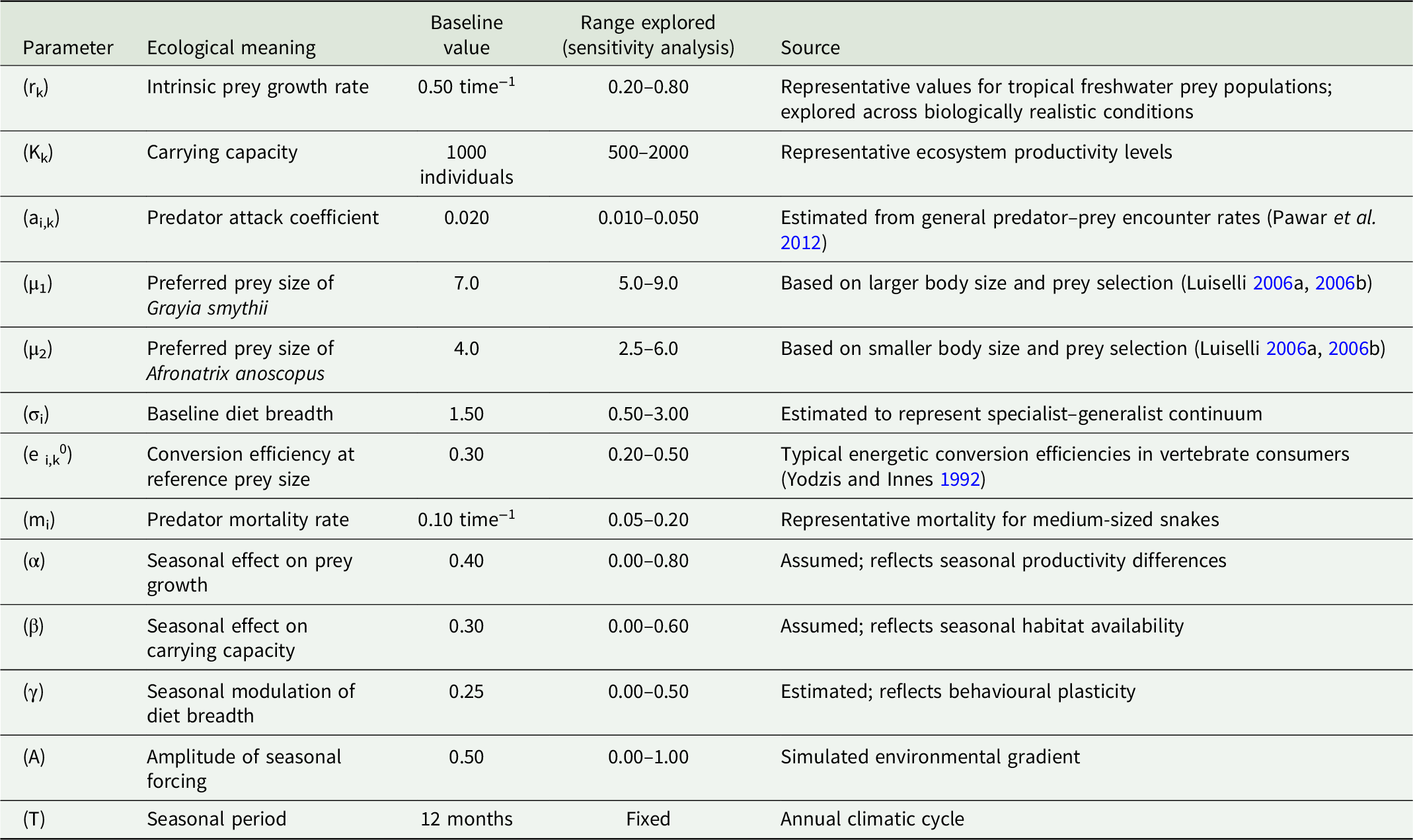
Each model parameter corresponds to a measurable ecological process (Table 1 and see Online Supplementary Table S1 for the potential empirical estimation). The intrinsic prey growth rate (r k ) determines the rate at which prey populations increase in the absence of predation, whereas the carrying capacity (K k ) represents the maximum abundance sustainable under prevailing environmental conditions. Both parameters vary seasonally according to changes in ecosystem productivity. Predator attack coefficients (a i,k ) describe the probability of successful encounters between predators and prey independently of prey-size preferences. In contrast, prey-size selection is governed exclusively by the Gaussian preference kernel through the parameters μ i (preferred prey size) and σ i (diet breadth). Conversion efficiency (e i,k (x)) quantifies the proportion of prey abundance converted into predator population growth. Unlike traditional formulations assuming constant energetic returns within prey categories, conversion efficiency is explicitly allowed to vary with prey body size because prey of different sizes provide different energetic rewards and handling costs. Finally, predator mortality (m i ) integrates background mortality from senescence, disease, and predation independently of food availability.
Model parameters used in simulations. Conversion efficiency varies with prey body size according to ei,k(x) = ei,k 0(x/xref), with xref = 5.5 size units. The units are: r = time−1, K = individuals, a = derived attack-rate units, μ = size units, σ = size units, e = dimensionless, m = time−1, α, β, γ, A = dimensionless, and T = months

Table 1. Long description
A table with 13 rows and 4 columns. The columns are labeled Parameter, Ecological meaning, Baseline value, Range explored (sensitivity analysis), and Source. The table lists various model parameters used in simulations, including intrinsic prey growth rate, carrying capacity, predator attack coefficient, preferred prey size, baseline diet breadth, conversion efficiency, predator mortality rate, seasonal effects, and amplitude of seasonal forcing. Each parameter is described with its ecological meaning, baseline value, range explored for sensitivity analysis, and the source of the values. The parameters are listed with their respective units, such as time inverse, individuals, derived attack-rate units, size units, dimensionless, and months.
For tropical predator communities, including freshwater snakes such as G. smythii and A. anoscopus, empirical parameterization could be achieved by combining independent datasets on predator diet composition, prey-size distributions, prey abundance, and habitat-specific seasonal variation in productivity. Because all parameters may not be simultaneously available for a given system, the framework is designed to evaluate ecological mechanisms through parameter exploration rather than requiring complete species-specific calibration. To assess robustness against parameter uncertainty, I performed global sensitivity analyses across biologically realistic parameter ranges, identifying which ecological processes most strongly influence coexistence outcomes.
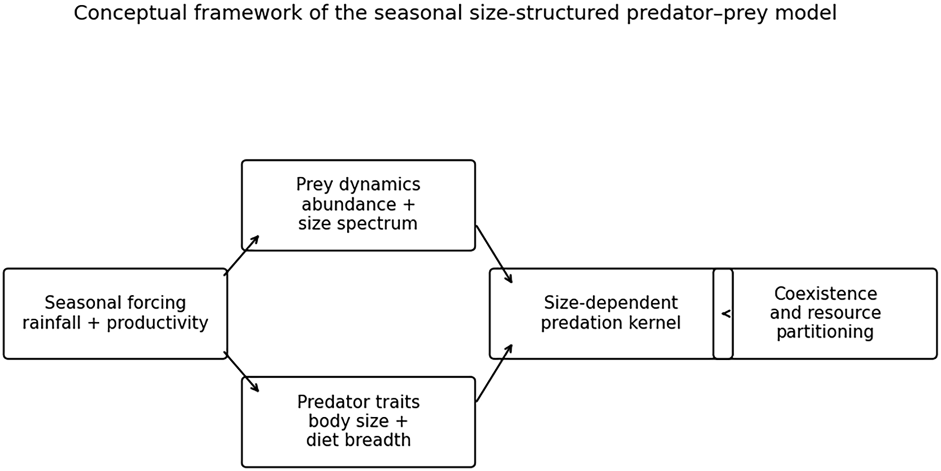
The conceptual framework of the model is given in Figure 1. This figure was generated to illustrate the conceptual structure of the model; all quantitative predictions were obtained from numerical simulations described below.
Conceptual framework of the seasonal size-structured predator–prey model. The model integrates seasonal environmental forcing, prey population dynamics, predator functional traits, and size-dependent predation to explain resource partitioning and predator abundance balance among sympatric generalist predators. Seasonal variation affects prey productivity, carrying capacity, predator activity, and dietary flexibility. Prey are represented along a continuous body-size axis, whereas predators interact with prey through species-specific size-selection kernels determined by predator morphology and foraging strategy. The connecting element between the size-dependent predation kernel and the final outcome represents the resulting degree of resource overlap and its translation into resource partitioning and predator abundance balance. The emergent outcome is therefore determined by dynamic resource partitioning rather than fixed dietary specialization.

Numerical implementation
For numerical simulations, the continuous prey-size distribution is discretized into J size classes:
 $n_{k,j}\left(t\right)$
Where j = 1,…,J. Consumption becomes:
 $C_{i,k,j}(t)=a_{i,k,j}(t)S_{i}(t)n_{k,j}(t)\phi _{i,j}$
The discrete formulation allows efficient numerical integration and facilitates sensitivity analysis across large parameter spaces.
The system of differential equations was solved numerically using a fourth-order Runge–Kutta integration scheme with adaptive time steps. Continuous prey-size distributions were discretized into equally spaced size classes, allowing numerical approximation of prey-size integrals while preserving the continuous nature of predator size selection.
Each simulation was initiated with randomly generated prey abundances within biologically realistic limits, whereas both predator populations were initialized at equal abundances (100 individuals per predator species), and simulations were run until predator and prey populations reached dynamic equilibrium or stable periodic oscillations. To ensure that transient dynamics did not influence the results, only the final portion of each simulation was retained for subsequent analyses.
To quantify predator balance and absolute persistence, I used two complementary metrics. The balanced coexistence index (BCI) was calculated as
 $BCI=min\left[S_{1},S_{2}\right]/max\left[S_{1},S_{2}\right]$
Where S 1 and S 2 are the abundances of the two predator species. The BCI ranges from 0, indicating complete competitive asymmetry, to 1, indicating equal predator abundances. BCI was calculated at the end of the simulation as the ratio between the abundance of the less abundant and the more abundant predator. As a complementary measure of absolute persistence, minimum predator abundance (MPA) was calculated as the minimum abundance of either predator during the final simulation period. Thus, BCI quantifies relative abundance balance, whereas MPA quantifies absolute abundance of the rarer predator. A high BCI therefore indicates balanced persistence of the two predator populations but does not by itself demonstrate asymptotic coexistence under all possible perturbations.
For the numerical simulations presented here, K = 1 prey category was represented as a continuous prey-size distribution discretized into 20 size classes. Unless otherwise stated, all reported values represent means ± standard deviations calculated from the final simulation period after excluding the burn-in phase.
Simulation scenarios
To investigate the mechanisms promoting predator coexistence, four complementary simulation experiments were performed.
Scenario 1 . Predator preferred prey-size divergence. The difference between predator-preferred prey sizes (μ 1 −μ 2) was progressively increased while all remaining parameters were held constant. This experiment tested the hypothesis that increasing body-size divergence promotes coexistence through partial resource partitioning. Predicted response variables included: dietary overlap, predator abundance, and coexistence probability. Coexistence probability is the proportion of simulations in which both predators remained > 1. In this case, dietary overlap between predators (O) was quantified as the overlap between their prey-size exploitation kernels using the overlap coefficient:
 $O=\int min[\phi _{1}(x),\phi _{2}(x)]dx$
where values close to one indicate extensive overlap in prey-size use, whereas values close to zero indicate strong resource partitioning.
Scenario 2. Seasonal environmental forcing. Seasonality amplitude (A) was varied from constant environmental conditions (A = 0) to strongly seasonal environments. This scenario examined whether seasonal fluctuations modify prey availability sufficiently to alter predator coexistence. Measured outputs included: prey abundance, predator abundance, temporal variation in diet breadth, and niche overlap.
Scenario 3 . Ecosystem productivity. Baseline prey productivity (r k ) and carrying capacity (K k ) were independently varied across wide ecological ranges. This experiment evaluated whether coexistence depends primarily on resource abundance or on predator size differentiation. Outputs included long-term predator persistence, extinction probability, and community abundance. Predator persistence was recorded when the minimum abundance of both predator populations remained above one individual throughout the simulation. Predator extinction was recorded when the abundance of either predator declined below one individual during the simulation. Extinction probability was calculated as the proportion of simulations resulting in predator extinction. Total community abundance was calculated as the sum of prey and predator abundances at the end of each simulation.
Scenario 4 . Dietary flexibility. Baseline niche width (σ i ) and seasonal flexibility (γ i ) were varied independently. Small values represent specialized predators, whereas larger values correspond to increasingly generalist foraging strategies. This simulation tested whether flexible prey-size selection stabilizes coexistence under fluctuating environmental conditions.
For each ecological scenario, 100 replicate simulations were performed using identical environmental conditions but independent initial population states. For factorial simulations, parameter combinations were evaluated on regular grids spanning the explored parameter ranges. Heatmaps were generated using the mean BCI calculated for each parameter combination. The reported coexistence index values represent means ± standard deviations across replicates.
All simulations were performed in Python 3.11 using numerical integration of the coupled predator–prey differential equations. The model was solved using the adaptive Runge–Kutta method implemented in the solve_ivp function of the SciPy library, with an explicit fourth-order Runge–Kutta algorithm and adaptive time-step control to ensure numerical stability. Simulations were run for 120 temporal units (months), corresponding to a 10-year period, with model outputs recorded at regular monthly intervals. A preliminary 20-month burn-in period was excluded from summary statistics to avoid potential effects associated with initial conditions. Increasing the simulation duration to 240 months produced qualitatively identical patterns, indicating that the observed coexistence outcomes were not dependent on the selected temporal window.
For each simulation, prey abundance was initially distributed across 20 continuous body-size classes, representing the available prey-size spectrum within the community. Predator populations were initialized at equal abundances (100 individuals per predator species), and simulations were repeated under different ecological scenarios to evaluate the effects of resource partitioning, environmental variability, and parameter uncertainty.
Unless otherwise specified, time is expressed in months, abundance in individuals, and prey body size in internally consistent arbitrary size units. Dimensioned parameters are expressed in the corresponding derived units of the model equations.
The baseline model used intermediate parameter values within biologically realistic ranges. For the scenario simulations, parameter values were varied within the following ranges: predator prey-size preferences (μ) between 2 and 8 size units, prey-size niche breadth (σ) between 0.5 and 3.0, attack coefficients (a) between 0.010 and 0.050, conversion efficiencies at the preference prey size (e$) between 0.10 and 0.30, mortality rates (m) between 0.10 and 0.40, intrinsic prey growth rates (r) between 0.4 and 1.0, and prey carrying capacity/resource availability (K) between 200 and 1500 abundance units.
Sensitivity analysis
To evaluate the robustness of model predictions, a global sensitivity analysis was performed using Latin Hypercube Sampling (LHS). Parameter values were simultaneously sampled across biologically plausible ranges, thereby generating a broad spectrum of ecological scenarios without assuming any particular combination of parameter values. For the LHS sensitivity analysis, parameter values were sampled independently within the ranges specified in Table 1. For each parameter set, the model was simulated over the full simulation period, allowing predator and prey populations to reach either equilibrium or stable periodic dynamics. The following response variables were recorded: (i) coexistence probability; (ii) predator equilibrium abundance; (iii) prey abundance; (iv) dietary overlap; (v) temporal variability in predator populations. Temporal variability was quantified as the coefficient of variation (CV) of predator abundance during the final simulation period. Spearman rank correlation coefficients (ρ) were calculated to quantify the strength and direction of the association between each model parameter and the corresponding coexistence metrics. Parameters were subsequently ranked according to the absolute magnitude of their correlation coefficients. To ensure convergence of parameter estimates, 10,000 independent simulations were performed for the LHS sensitivity analysis. Statistical significance was assessed at α = 0.05.
Model predictions
Rather than fitting empirical observations, the purpose of the simulations was to evaluate whether the proposed ecological mechanisms generate consistent theoretical predictions. Specifically, the model predicts that:
-
1. increasing differences in predator body size reduce dietary overlap through shifts in preferred prey-size distributions;
-
2. coexistence remains robust across wide parameter ranges provided that predators differ sufficiently in preferred prey-size spectra.
These predictions constitute explicit hypotheses that can be tested using long-term dietary datasets from tropical predator assemblages.
Results
Baseline dynamics of the size-structured predator–prey system
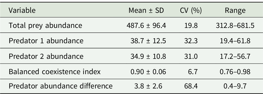
The baseline simulation produced persistent predator–prey oscillations throughout the simulation period (Figure 2). Both predator species persisted under baseline conditions despite pronounced seasonal fluctuations in prey abundance, resulting in a high BCI (Table 2). Temporal variability was substantial in both prey and predator populations, with predator abundances showing greater coefficients of variation than prey abundance.
Baseline dynamics of prey and predator populations generated by the seasonal size-structured predator–prey model. The simulation shows temporal changes in total prey abundance and predator abundance over multiple seasonal cycles under baseline parameter values. Seasonal forcing generates periodic fluctuations in prey availability, followed by delayed responses in predator populations. Despite temporal variation in resource abundance, both predator species persist throughout the simulation. The lower panel shows the prey-size distribution used to represent the continuous resource spectrum. Panels: upper = total prey abundance through time; middle = predator population trajectories; lower = prey-size distribution.

Baseline simulation output. Abundance is expressed in terms of number of individuals. SD = standard deviation; CV = coefficient of variation

Table 2. Long description
The table presents data on ecological variables, including total prey abundance, predator 1 abundance, predator 2 abundance, balanced coexistence index, and predator abundance difference. It has five rows and four columns. The columns are labeled Variable, Mean ± SD, CV (%), and Range. Row 1: Total prey abundance, Mean ± SD: 487.6 ± 96.4, CV (%): 19.8, Range: 312.8–681.5. Row 2: Predator 1 abundance, Mean ± SD: 38.7 ± 12.5, CV (%): 32.3, Range: 19.4–61.8. Row 3: Predator 2 abundance, Mean ± SD: 34.9 ± 10.8, CV (%): 31.0, Range: 17.2–56.7. Row 4: Balanced coexistence index, Mean ± SD: 0.90 ± 0.06, CV (%): 6.7, Range: 0.76–0.98. Row 5: Predator abundance difference, Mean ± SD: 3.8 ± 2.6, CV (%): 68.4, Range: 0.4–9.7.
Predator trait divergence determines coexistence strength
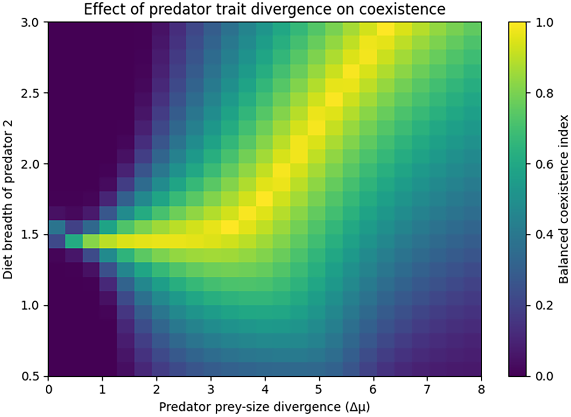
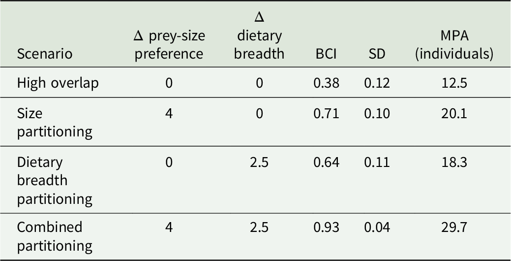
The factorial simulations showed that predator differentiation in prey-size use strongly influenced both balanced and absolute predator abundance (Figures 3 and 4). When predators exploited similar prey-size classes (Δμ = 0), the BCI was low (0.38 ± 0.12), indicating strong competitive asymmetry (Table 3). Increasing divergence in prey-size preference progressively increased the BCI, which reached 0.71 ± 0.10 under size partitioning and 0.93 ± 0.04 under combined differentiation in prey-size preference and dietary breadth (Table 3).
Effect of predator trait divergence on coexistence dynamics. The heatmap shows the outcome of factorial simulations exploring the combined effects of predator differences in preferred prey size (Δμ) and dietary niche width on coexistence dynamics. Each cell represents the balanced coexistence index calculated from the mean predator abundances during the final simulation period, defined as the ratio between the less abundant and the more abundant predator population (min (P 1 ,P 2)/max (P 1 ,P 2)). Values close to one indicate stable coexistence with similar predator abundances, whereas values approaching zero indicate strong competitive asymmetry and potential exclusion. The simulations show that increasing divergence in prey-size exploitation reduces competitive overlap and promotes more balanced coexistence between sympatric generalist predators.

Effects of predator trait divergence on balanced abundance and absolute predator abundance. The two panels show the outcomes of simulations exploring four combinations of divergence in preferred prey size (Δμ) and dietary breadth. (A) Balanced coexistence index (BCI), calculated as the ratio between the abundance of the less abundant and more abundant predator during the final simulation period; values close to one indicate similar predator abundances, whereas values approaching zero indicate strong competitive asymmetry. Bars represent means ± SD across replicate simulations. (B) Minimum predator abundance (MPA), defined as the minimum abundance reached by either predator during the final simulation period, providing a complementary measure of absolute abundance that is not captured by the BCI. Increasing divergence in prey-size preference and dietary breadth generally increased both abundance balance and the absolute abundance of the less abundant predator, with the strongest effect occurring when both dimensions were differentiated.

Trait-divergence simulation experiment. Values represent means ± SD from 100 replicate simulations. Δ prey-size preference represents the difference between predator-preferred prey sizes, whereas Δ dietary breadth represents the difference in predator prey-size niche breadth. BCI = balanced coexistence index, calculated as the ratio between the abundance of the less abundant and more abundant predator; MPA = minimum predator abundance, defined as the minimum abundance reached by either predator during the final simulation period. Higher BCI values indicate more balanced predator abundances, whereas higher MPA values indicate greater absolute abundance of the less abundant predator

Table 3. Long description
A table with four rows and five columns comparing different predator differentiation scenarios and their effects on predator abundance. The columns are labeled Scenario, Δ prey-size preference, Δ dietary breadth, BCI, SD, and MPA (individuals). The rows are labeled High overlap, Size partitioning, Dietary breadth partitioning, and Combined partitioning. Each row provides values for the different metrics under each scenario. For High overlap, the values are 0, 0, 0.38, 0.12, and 12.5. For Size partitioning, the values are 4, 0, 0.71, 0.10, and 20.1. For Dietary breadth partitioning, the values are 0, 2.5, 0.64, 0.11, and 18.3. For Combined partitioning, the values are 4, 2.5, 0.93, 0.04, and 29.7.
The complementary analysis of MPA showed a similar overall pattern, although the response was not strictly monotonic across individual partitioning scenarios (Figure 4). MPA increased from 12.5 ± 4.0 individuals under high overlap to 20.1 ± 6.0 individuals under size partitioning. Dietary breadth partitioning produced an intermediate MPA of 18.3 ± 5.5 individuals, whereas combined partitioning resulted in the highest MPA (29.7 ± 2.5 individuals). Thus, the increase in BCI associated with trait differentiation was accompanied by higher absolute abundance of the less abundant predator, particularly when differences in prey-size preference and dietary breadth were combined (Table 3). A Spearman correlation between prey-size divergence and BCI showed a strong positive relationship (ρ = 0.86, P < 0.001), indicating that increasing separation in prey-size exploitation was strongly associated with greater predator abundance balance.
Effects of seasonality and prey productivity
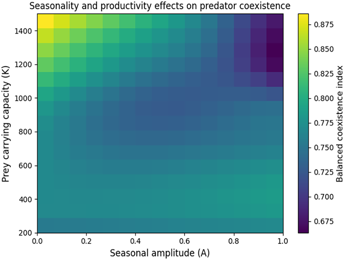
Environmental simulations showed that prey carrying capacity strongly influenced predator coexistence across all levels of seasonal forcing (Figure 5). At low carrying capacity (K = 200), predator populations became increasingly asymmetric, yielding a mean BCI of 0.52 ± 0.15. In contrast, increasing prey carrying capacity/resource availability (K = 1500) promoted substantially more balanced coexistence (0.88 ± 0.07). Seasonal forcing alone had relatively little effect on predator balance, but its interaction with prey productivity became evident under resource-limited conditions, where seasonal fluctuations amplified competitive asymmetry (Figure 5).
Effects of seasonal environmental variability and prey productivity on predator coexistence dynamics. The heatmap shows the balanced coexistence index obtained from factorial simulations across gradients of seasonal forcing amplitude and prey carrying capacity. Each cell represents the ratio between the less abundant and the more abundant predator population during the final simulation period (min(P 1 ,P 2 )/max(P 1 ,P 2 )), with values close to one indicating balanced coexistence and values approaching zero indicating strong competitive asymmetry. Seasonal variability modifies predator coexistence by altering temporal fluctuations in prey availability, while increased prey productivity generally increases predator persistence. The simulations indicate that environmental seasonality alone does not determine coexistence but interacts with resource availability to influence the stability of competing generalist predators.

Sensitivity analysis identifies key determinants of coexistence
Global sensitivity analysis identified prey-size divergence as the strongest determinant of coexistence, followed by dietary breadth differentiation and prey carrying capacity (Figure 6). Demographic parameters such as attack rate and mortality had comparatively weaker effects.
Global sensitivity analysis of predator abundance balance. Bars show Spearman rank correlation coefficients (ρ) between model parameters and predator abundance balance. Positive values indicate positive associations with abundance balance, whereas negative values indicate negative associations. Prey-size divergence showed the strongest positive association, followed by dietary breadth divergence, prey carrying capacity, and conversion efficiency, whereas attack rate and mortality showed weaker negative associations. The corresponding P-values are reported above each bar. Parameter values were sampled across biologically plausible ranges, and 10,000 independent simulations were performed.

Alternative ecological scenarios
Predator trajectories differed markedly among ecological scenarios (Figure 7). High dietary overlap resulted in strong competitive asymmetry, whereas increasing divergence in prey-size preference and dietary breadth progressively promoted balanced predator abundance. Under high dietary overlap, predator populations diverged rapidly, with predator 1 reaching a final abundance of 62.4 individuals compared with 14.7 individuals for predator 2. The resulting BCI was only 0.24. Size partitioning increased BCI to 0.74, while dietary breadth differentiation produced an intermediate response (0.67). The combined partitioning scenario generated the most balanced outcome, with final abundances of 41.2 and 38.6 individuals, corresponding to a BCI of 0.94.
Predator population trajectories under alternative resource-partitioning scenarios. Predator abundances are shown through time under four scenarios of resource use: (A) high dietary overlap, (B) prey-size partitioning, (C) dietary breadth differentiation, and (D) combined differentiation in prey-size preference and dietary breadth. The high-overlap scenario produces marked competitive asymmetry, whereas resource partitioning reduces the difference in predator abundance. BCI values shown in each panel represent the balanced coexistence index calculated from predator abundances at the end of the simulation. Solid and dashed lines represent predator 1 and predator 2, respectively. Only a single representative simulation trajectory is used for this figure.

Figure 7. Long description
The image contains four line graphs showing predator population trajectories under different resource-partitioning scenarios. Each graph represents a different scenario of resource use: high dietary overlap, prey-size partitioning, dietary breadth differentiation, and combined differentiation in prey-size preference and dietary breadth. Panel A: The line graph shows predator abundance over simulation time under high dietary overlap. The y-axis represents predator abundance in individuals, and the x-axis represents simulation time. Predator 1 is represented by a solid blue line, and Predator 2 is represented by a dashed orange line. The BCI value is 0.24. Predator 1 shows a higher and increasing abundance, while Predator 2 shows a lower and decreasing abundance. Panel B: The line graph shows predator abundance over simulation time under prey-size partitioning. The y-axis represents predator abundance in individuals, and the x-axis represents simulation time. Predator 1 is represented by a solid blue line, and Predator 2 is represented by a dashed orange line. The BCI value is 0.74. Both predators show relatively stable abundances, with Predator 1 having a slightly higher abundance than Predator 2. Panel C: The line graph shows predator abundance over simulation time under dietary breadth differentiation. The y-axis represents predator abundance in individuals, and the x-axis represents simulation time. Predator 1 is represented by a solid blue line, and Predator 2 is represented by a dashed orange line. The BCI value is 0.67. Predator 1 shows a higher and relatively stable abundance, while Predator 2 shows a lower and relatively stable abundance. Panel D: The line graph shows predator abundance over simulation time under combined differentiation in prey-size preference and dietary breadth. The y-axis represents predator abundance in individuals, and the x-axis represents simulation time. Predator 1 is represented by a solid blue line, and Predator 2 is represented by a dashed orange line. The BCI value is 0.94. Both predators show relatively stable and similar abundances.
Mechanistic basis of size-mediated coexistence
The exploitation-kernel analysis demonstrated that coexistence emerged from partial segregation of prey-size use (Figure S2). Under maximum overlap conditions, predator kernels showed an overlap coefficient of 0.82, whereas divergence in prey-size preference reduced overlap to 0.29.
The relationship between kernel overlap and BCI was strongly negative (ρ = −0.88, P < 0.001), indicating that reduced direct competition through size-mediated resource partitioning was strongly associated with greater predator abundance balance.
Discussion
Advances over previous predator–prey models
The main contribution of this framework is the integration of three components that are rarely considered simultaneously in predator–prey coexistence models: continuous prey-size structure, predator-specific exploitation kernels, and seasonal environmental forcing. Traditional consumer–resource models (for instance, Lotka–Volterra equations) often represent resources as homogeneous entities and describe species interactions through fixed coefficients, which may overlook how variation in prey traits and predator resource-use strategies influences competitive outcomes (Burton Reference Burton2005). In contrast, the present model explicitly represents prey body size as a continuous trait and links predator feeding rates to size-dependent exploitation functions, allowing competitive interactions to emerge from differences in resource use rather than from predefined competition coefficients.
A further innovation is the integration of seasonal forcing within a size-structured coexistence framework. Instead of treating environmental variability as an external disturbance, the model incorporates seasonal changes in prey productivity, carrying capacity, predator activity, and dietary flexibility, thereby allowing environmental conditions to modify both resource availability and interaction strength. This approach provides a mechanistic explanation of how temporal variability can alter the balance between competitive exclusion and coexistence.
The simulation experiments extend these mathematical assumptions by systematically exploring how variation in prey-size divergence, dietary breadth, and resource availability affects coexistence outcomes. Rather than identifying a single coexistence threshold, the model reveals how multiple ecological mechanisms interact to determine predator persistence and competitive balance. This combination of trait-based structure and dynamic environmental forcing represents a flexible framework for investigating coexistence in predator communities characterized by high dietary overlap.
Although the model incorporates several interacting processes, each component was included to represent a specific ecological mechanism: prey-size distributions describe resource structure, exploitation kernels describe predator resource use, and seasonal forcing represents temporal variation in resource availability and interaction strength. This combination of trait-based structure and dynamic environmental forcing represents a flexible framework for investigating coexistence in predator communities characterized by high dietary overlap.
Size-mediated resource partitioning and predator coexistence
The size-structured predator–prey model developed in this study suggests that balanced persistence of sympatric generalist predators can emerge through partial differentiation in resource use rather than complete dietary segregation. In the simulations, predator differentiation in prey-size exploitation and dietary breadth increased abundance balance, whereas extensive overlap increased competitive asymmetry. Importantly, the complementary analysis of MPA showed that this pattern was not restricted to relative abundance balance. Minimum predator abundance increased from 12.5 ± 4.0 individuals under high overlap to 29.7 ± 2.5 individuals under combined partitioning, indicating that greater trait differentiation was associated not only with more similar predator abundances but also with a higher absolute abundance of the less abundant predator. These patterns emerged from the mathematical structure of the model, in which predator dynamics were determined by the balance between energetic gains from size-structured prey consumption and mortality losses. Because prey were represented along a continuous size spectrum, predator-specific exploitation kernels determined the extent of overlap in prey-size use, thereby shaping prey consumption and predator population dynamics.
When predators exploited similar portions of the prey-size spectrum, one species progressively dominated the interaction, whereas divergence in prey-size preferences reduced competitive imbalance and increased the absolute abundance of the less abundant predator. The strongest response occurred when divergence in prey-size preference was combined with differentiation in dietary breadth, suggesting that multiple dimensions of resource differentiation can reinforce one another in reducing competitive asymmetry. This result is consistent with classical niche theory, which predicts that differentiation in resource use can reduce interspecific competition (Chesson Reference Chesson2000; Schoener Reference Schoener1974), while also supporting the view that complete niche separation is not required for coexistence if partial differences in resource exploitation are sufficient to generate stabilizing effects (Chesson Reference Chesson2000; Murphy et al. Reference Murphy, Pecl, Everett, Heneghan, Richards, Richardson and Blanchard2023; Nakazawa et al. Reference Nakazawa, Ohba and Ushio2013).
Body size is widely recognized as an important axis of ecological differentiation because it influences predator–prey interactions, energetic requirements, and patterns of resource exploitation (McGill et al. Reference McGill, Enquist, Weiher and Westoby2006; Peters Reference Peters1986; Woodward et al. Reference Woodward, Ebenman, Emmerson, Montoya, Olesen, Valido and Warren2005). The results of this model extend this perspective by showing that prey body-size distributions can influence predator abundance balance and absolute persistence even when predators share the same prey assemblage. Size-structured approaches have previously demonstrated that variation in prey size can alter competitive outcomes among consumers by modifying encounter rates, feeding efficiency, and energetic gains (De Roos et al. Reference De Roos, Schellekens, Van Kooten and Persson2008; Persson et al. Reference Persson, Andersson, Wahlstrom and Eklov1996). By explicitly incorporating prey size as a continuous trait, the present framework provides a mechanistic representation of how subtle differences in resource use may influence both competitive balance and the absolute abundance of competing predators.
The role of resource availability and seasonal forcing
As expected, in our simulations, resource availability further modified the strength of competitive interactions. Increasing prey carrying capacity consistently promoted more balanced predator abundances, whereas resource limitation increased competitive asymmetry. This result agrees with ecological theory predicting that competition becomes stronger when resources are scarce and limiting factors become more intense (Ricklefs and Miller Reference Ricklefs and Miller2000). Under conditions of high productivity, predators may tolerate greater overlap in resource use because sufficient prey availability reduces the strength of exploitative competition (Amarasekare Reference Amarasekare2008; Chesson Reference Chesson and Wang2012; Holt et al. Reference Holt, Grover and Tilman1994). Conversely, when resources are limited, differences in prey-size exploitation and dietary breadth become increasingly important in determining competitive outcomes (Ricklefs et al. Reference Ricklefs2010; Ricklefs and Miller Reference Ricklefs and Miller2000). A high BCI should therefore be interpreted as evidence of balanced predator abundance rather than as definitive evidence of asymptotic coexistence because relative abundance balance does not by itself guarantee long-term persistence under all environmental perturbations.
Seasonal environmental variation influenced coexistence primarily through its interaction with resource availability rather than through direct effects alone. Seasonal fluctuations in tropical ecosystems frequently affect population dynamics by modifying resource production, consumer activity, and trophic interactions (Richards and Coley Reference Richards and Coley2007; Wolda Reference Wolda1992). The model suggests that environmental variability may amplify competitive asymmetry when prey availability is low, whereas its effects may be buffered when resources are abundant. This supports the view that temporal variation should be considered together with species traits rather than as an independent driver of community dynamics.
Implications for tropical predator communities
These findings have implications for understanding coexistence among tropical predators, particularly aquatic snakes with overlapping diets. The model was motivated by the sympatric African water snakes G. smythii and A. anoscopus, which occupy similar habitats and exploit comparable prey resources but differ in body size and prey-use patterns (Luiselli Reference Luiselli2006b). Although the model is not intended to reproduce the complete ecology of these species, it provides a theoretical framework for evaluating how differences in prey-size exploitation and dietary breadth may contribute to balanced predator persistence when direct dietary overlap is high. The distinction between balanced abundance and absolute abundance is important in this context: the model predicts that resource differentiation can simultaneously reduce competitive asymmetry and increase the abundance of the less abundant predator, but these theoretical outcomes do not constitute empirical evidence that prey-size partitioning is the mechanism maintaining coexistence in the focal snake species. Similar mechanisms may apply to other predator assemblages in which species share prey resources but differ in morphological or behavioural traits affecting resource acquisition (Luiselli Reference Luiselli2006b; Rabe et al. Reference Rabe, Binder, Anton, Meyer, Metz, Smith and Stahler2025).
The model also provides testable predictions for empirical studies. If prey-size partitioning contributes to balanced persistence (Rudolf Reference Rudolf2008, Říha et al. Reference Říha, Vejřík, Rabaneda-Bueno, Jarić, Prchalová, Vejříková and Peterka2025), sympatric predators should exhibit differences in prey-size distributions despite overlap in prey identity. These predictions can be evaluated through long-term dietary datasets, stable isotope analyses, metabarcoding approaches, and direct measurements of prey selection. Such approaches would allow assessment of whether the patterns predicted by the model – including reduced prey-size overlap, greater abundance balance, and higher abundance of the less abundant predator – occur in natural communities and under different environmental conditions.
Model limitations and future perspectives
As with all theoretical models, several assumptions should be considered when interpreting these results. The framework focuses on size-mediated resource use and seasonal environmental forcing, while other factors that may influence predator coexistence, including spatial heterogeneity, behavioural interference, predator movement, and evolutionary adaptation, are not explicitly represented. Nevertheless, simplifying these additional mechanisms allows the model to isolate the contribution of prey-size structure and resource availability to coexistence dynamics. Moreover, both BCI and MPA are outcome metrics rather than direct measures of asymptotic coexistence and therefore should be interpreted as indicators of competitive balance and predator persistence within the simulated time frame. Future extensions incorporating spatial variation, adaptive behaviour, or additional trophic interactions could provide further insights into the mechanisms maintaining predator diversity.
Overall, this study demonstrates the value of integrating continuous prey traits, predator-specific resource-use strategies, and environmental variability within a unified modelling framework. The results suggest that balanced persistence among tropical predators may emerge from interactions between stabilizing mechanisms associated with resource differentiation and environmental conditions that regulate competition intensity. These results represent mechanistic theoretical predictions rather than empirical demonstrations of the processes maintaining coexistence in natural predator communities. By explicitly linking prey-size structure with seasonal dynamics, this approach contributes to a more mechanistic understanding of how resource differentiation may promote predator persistence in species-rich tropical ecosystems.
Supplementary material
The supplementary material for this article can be found at https://doi.org/10.1017/S0266467426100789.
Data availability statement
This study does not include original empirical data, as all results are derived from the mathematical model and numerical simulations described within the manuscript, and therefore no datasets were generated or deposited. The original dataset motivating this study is entirely available in Luiselli (Reference Luiselli2006a).
Author contribution
LL decided the subject and the method of manuscript, analysed the data; wrote the first draft of the manuscript and reviewed and approved the final draft.
Funding statement
None.
Competing interests
The author declares no conflict of interest.
Artificial intelligence
I have used AI tools (ChatGPT) in the writing process for this manuscript to enhance the English language and the logic of the manuscript, including the quality improvement of some figures. Every correction made by the AI has been checked carefully by myself.