1 Introduction
Detonation waves are supersonic waves that can propagate in various materials, including condensed matter, combustible gas mixtures and particle/droplet aerosols (Fickett Reference Fickett1985; Lee Reference Lee2008). In recent years, detonation research has attracted more and more attention due to its potential application in aerospace propulsion (Kailasanath Reference Kailasanath2003; Wolanski Reference Wolanski2013). Three kinds of detonation engines, i.e. pulse detonation engine (PDE), rotating detonation engine (RDE) and oblique detonation engine (ODE), have been proposed and studied widely. The ODE is one kind of ramjet engine based on an oblique detonation wave (ODW), which is suitable for air-breathing hypersonic aircraft. The development of ODE requires a better understanding of oblique detonation dynamics, particularly on the interaction of supersonic inflow and oblique shock-induced heat release.
In the literature, there have been extensive investigations of ODWs beginning with the early theoretical studies of steady ODWs initiated from semi-infinite wedges using shock and detonation polar curves for determining different wave angles (e.g. Gross Reference Gross1963; Pratt, Humphrey & Glenn Reference Pratt, Humphrey and Glenn1991; Ashford & Emanuel Reference Ashford and Emanuel1994; Emanuel & Tuckness Reference Emanuel and Tuckness2004). Later studies then focused on the formation structure of ODWs and their subsequent evolution. The pioneering work of Li, Kailasanath & Oran (Reference Li, Kailasanath and Oran1994) presented the first simulation of this structure, which is shown to consist of a non-reactive oblique shock, an induction region, a set of deflagration waves and the oblique detonation surface. More recent studies also showed that there exist other types of oblique shock-to-detonation transition structure depending on different chemical and aerodynamic parameters. The underlying mechanism of these different transition types has been studied by numerical simulations and theoretical analyses (Choi, Shin & Jeung Reference Choi, Shin and Jeung2009; Teng & Jiang Reference Teng and Jiang2012; Teng, Jiang & Ng Reference Teng, Jiang and Ng2014; Liu et al. Reference Liu, Wu, Yao and Wang2015, Reference Liu, Liu, Wu and Wang2016; Yang et al. Reference Yang, Teng, Jiang and Ng2018). Besides the initiation structure, the surface instability features of ODWs are also widely studied. Cellular ODW surfaces with triple points have been demonstrated by numerical simulations (Papalexandris Reference Papalexandris2000) and observed experimentally as well (Viguier, Gourara & Desbordes Reference Viguier, Gourara and Desbordes1998). It is found that combustible mixtures with large value of activation energy are more susceptible to transverse waves or triple point formation (Papalexandris Reference Papalexandris2000). Choi et al. (Reference Choi, Kim, Jeung, Ma and Yang2007) showed several cellular structures with different activation energies and pointed out that these structures cannot be captured without enough numerical grid resolution. By using high-order numerical schemes and extending the computational domain sufficiently long for the instability to develop, recent numerical simulations further confirm the existence of cellular structures and their evolution processes (Verreault, Higgins & Stowe Reference Verreault, Higgins and Stowe2013; Teng et al. Reference Teng, Ng, Li, Luo and Jiang2015).
The aforementioned studies employ a two-dimensional (2-D) semi-infinite wedge in the homogeneous inflow. Using a realistic geometric configuration, rather than the ideal 2-D semi-infinite wedge, is also the subject of a number of recent investigations. The finite wedge or double wedge, which introduces an expansion wave in the initiation region or detonation product, is found to change the interaction of supersonic inflow and oblique shock-induced heat release (Qin & Zhang Reference Qin and Zhang2018; Fang, Hu & Teng Reference Fang, Hu and Teng2018). ODWs induced by a conical shock or spherical projectiles are simulated to study the initiation structures and formation mechanisms (Ju, Masuya & Sasoh Reference Ju, Masuya and Sasoh1998; Maeda, Kasahara & Matsuo Reference Maeda, Kasahara and Matsuo2012; Maeda et al. Reference Maeda, Sumiya, Kasahara and Matsuo2013). Another setting of inflow inhomogeneity, considering the effects of non-ideal mixing, was simulated recently, illustrating several distorted reactive fronts (Iwata, Nakaya & Tsue Reference Iwata, Nakaya and Tsue2016, Reference Iwata, Nakaya and Tsue2017; Fang et al. Reference Fang, Hu, Teng, Jiang and Ng2017).
Although several aspects have been studied, the ODW in unsteady flow has not been thoroughly reported in the literature to the authors’ knowledge. Generally, two types of unsteady processes have been pointed out before. One is the ODW surface instability, generating the unsteady cellular evolution (Choi et al. Reference Choi, Kim, Jeung, Ma and Yang2007; Yang et al. Reference Yang, Teng, Ng and Jiang2019); and the other is a transient phenomenon related with low inflow Mach number inducing an unsteady initiation region (Yang et al. Reference Yang, Teng, Jiang and Ng2018). However, those unsteady dynamics exist inherently even in the steady inflow, and only a few studies have been performed to disturb the inflow and look at the ODW’s transient response. The isolated disturbed density regions, with abruptly changing parameters inside, were placed before the ODW to examine its resilience to inflow disturbance (e.g. Fusina, Sislian & Parent Reference Fusina, Sislian and Parent2005; Teng, Zhao & Jiang Reference Teng, Zhao and Jiang2007). By increasing or decreasing the incident flow angle abruptly, the evolution of ODWs is simulated to study the hysteresis phenomena of an ODW (Liu et al. Reference Liu, Wang, Xiao, Yan and Wang2018). Our recent study demonstrates a complicated wave transition, such as the isolated local explosion and distorted reactive front, when wedge angle changes abruptly (Zhang et al. Reference Zhang, Yang, Teng, Ng and Wen2018).
In this study, an ODW in unsteady flow is simulated numerically by imposing a periodic sinusoidal density/temperature disturbance on the inflow. The present investigation thus aims to elucidate the dynamic response of the ODW subject to the imposed disturbances considered. As a first step to introduce a continuous disturbance, we keep the inflow velocity and pressure constant, and only disturb the density/temperature with a sinusoidal function to model a simplified but generic unsteady flow. In particular, this study focuses on the cases with continuous (or multi-pulse) inflow variation, while cases with single-pulse inflow variation are also simulated to clarify whether the resulting phenomena are derived from the continuous disturbance. The formation of triple points on the surface is analysed, demonstrating that a continuous disturbance does not facilitate the formation of triple points, although the surface seems more unstable at a given instant of time. Based on the movement of the ODW reaction surface, three regimes with distinct behaviours are distinguished depending on the disturbance wavenumber, illustrating an overshooting oscillation never reported before.
2 Physical and mathematical model
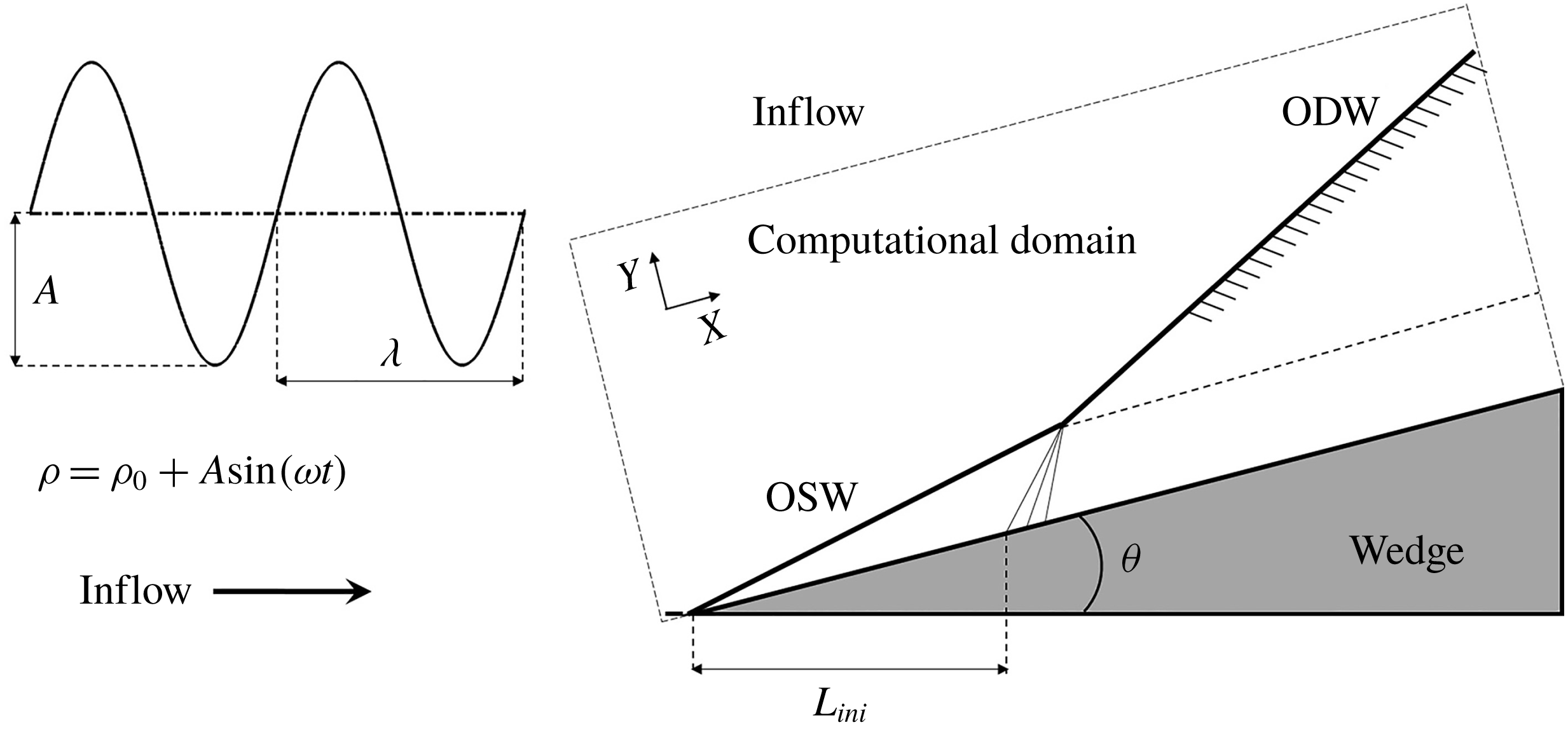
A schematic of a typical ODW induced by a 2-D, semi-infinite wedge is shown in figure 1. The presence of the wedge in a supersonic combustible inflow induces first an oblique shock wave (OSW). For a high inflow Mach number causing a high post-shock temperature behind the OSW, an exothermic chemical reaction begins, leading to ODW formation. As in previous computations, the coordinate is rotated to the direction along the wedge surface, and the Cartesian grid in the rectangular domain enclosed by the dashed line in figure 1 is aligned with the wedge surface.
Schematic of a typical ODW.

Following many previous studies (Grismer & Powers Reference Grismer and Powers1996; Papalexandris Reference Papalexandris2000; Choi et al.
Reference Choi, Kim, Jeung, Ma and Yang2007, Reference Choi, Shin and Jeung2009; Gui, Fan & Dong Reference Gui, Fan and Dong2011; Teng & Jiang Reference Teng and Jiang2012; Verreault et al.
Reference Verreault, Higgins and Stowe2013; Teng et al.
Reference Teng, Jiang and Ng2014; Yang et al.
Reference Yang, Teng, Jiang and Ng2018), the reactive Euler equations are used as governing equations for modelling the ODW flow field. To implement the two-step reaction model for chain-branching kinetics (Ng et al.
Reference Ng, Radulescu, Higgins, Nikiforakis and Lee2005), two additional reaction indices are introduced: one is the induction reaction index
 $\unicode[STIX]{x1D709}$
, and the other is the heat release index
 $\unicode[STIX]{x1D702}$
. The governing equations are
 $$\begin{eqnarray}\displaystyle & \displaystyle \frac{\unicode[STIX]{x2202}(\unicode[STIX]{x1D70C}\unicode[STIX]{x1D709})}{\unicode[STIX]{x2202}t}+\frac{\unicode[STIX]{x2202}(\unicode[STIX]{x1D70C}u\unicode[STIX]{x1D709})}{\unicode[STIX]{x2202}x}+\frac{\unicode[STIX]{x2202}(\unicode[STIX]{x1D70C}v\unicode[STIX]{x1D709})}{\unicode[STIX]{x2202}y}=H(1-\unicode[STIX]{x1D709})\unicode[STIX]{x1D70C}k_{I}\exp \left[E_{I}\left(\frac{1}{T_{S}}-\frac{1}{T}\right)\right], & \displaystyle\end{eqnarray}$$
 $$\begin{eqnarray}\displaystyle & \displaystyle \frac{\unicode[STIX]{x2202}(\unicode[STIX]{x1D70C}\unicode[STIX]{x1D702})}{\unicode[STIX]{x2202}t}+\frac{\unicode[STIX]{x2202}(\unicode[STIX]{x1D70C}u\unicode[STIX]{x1D702})}{\unicode[STIX]{x2202}x}+\frac{\unicode[STIX]{x2202}(\unicode[STIX]{x1D70C}v\unicode[STIX]{x1D702})}{\unicode[STIX]{x2202}y}=[1-H(1-\unicode[STIX]{x1D709})]\unicode[STIX]{x1D70C}(1-\unicode[STIX]{x1D702})k_{R}\exp \left[-\frac{E_{R}}{T}\right], & \displaystyle\end{eqnarray}$$
with the Heaviside step function
 $$\begin{eqnarray}H(1-\unicode[STIX]{x1D709})=\left\{\begin{array}{@{}ll@{}}1, & \unicode[STIX]{x1D709}\leqslant 1,\\ 0, & \unicode[STIX]{x1D709}>1.\end{array}\right.\end{eqnarray}$$
The specific total energy is thus expressed as
 $$\begin{eqnarray}e=\frac{p}{\unicode[STIX]{x1D70C}(\unicode[STIX]{x1D6FE}-1)}+\frac{1}{2}(u^{2}+v^{2})-\unicode[STIX]{x1D702}Q.\end{eqnarray}$$
The variables
 $\unicode[STIX]{x1D70C}$
,
 $u$
,
 $v$
,
 $p$
,
 $e$
and
 $Q$
are the density,
 $x$
-direction velocity,
 $y$
-direction velocity, pressure, specific total energy and the amount of chemical heat release, respectively. All the variables have been non-dimensionalized by reference to the uniform unburned state as follows:
 $$\begin{eqnarray}p=\frac{\widetilde{p}}{p_{0}},\quad \unicode[STIX]{x1D70C}=\frac{\widetilde{\unicode[STIX]{x1D70C}}}{\unicode[STIX]{x1D70C}_{0}},\quad T=\frac{\widetilde{T}}{T_{0}},\quad u=\frac{\widetilde{u}}{\sqrt{RT_{0}}},\quad v=\frac{\widetilde{v}}{\sqrt{RT_{0}}}.\end{eqnarray}$$
The dispersion-controlled dissipation (DCD) scheme (Jiang Reference Jiang2004) together with a third-order Runge–Kutta algorithm are used to approximate numerically the solutions of the governing equations. The DCD scheme is designed to adjust the dispersion around the strong discontinuity and thus non-physical oscillations near the shock wave are suppressed. Generally, it is one kind of total variation diminishing (TVD) schemes, which can achieve second-order accuracy in the smooth flow field. The main parameters are set to be
 $Q=50$
,
 $\unicode[STIX]{x1D6FE}=1.2$
,
 $E_{I}=5.0T_{s}$
and
 $E_{R}=1.0T_{s}$
, where
 $T_{s}$
is the post-shock temperature.
In this study, a steady ODW, with
 $M_{0}=10$
and
 $\unicode[STIX]{x1D703}=30^{\circ }$
, is first simulated as the initial flow field. These conditions correspond to the result of a smooth transition for the ODW initiation structure characterized by a curved shock (see Teng & Jiang Reference Teng and Jiang2012; Yang et al.
Reference Yang, Teng, Jiang and Ng2018, Reference Yang, Teng, Ng and Jiang2019). Once a steady ODW is established, a periodic sinusoidal density/temperature disturbance enters the computational domain through the left and upper boundaries. These two boundaries are prescribed as inflow boundary conditions, where the thermodynamic parameters at different instants are set according to the formula
 $\unicode[STIX]{x1D70C}=\unicode[STIX]{x1D70C}_{0}+A\sin (\unicode[STIX]{x1D714}t)$
. In the simulations, the parameters along the line perpendicular to the inflow direction are kept the same, by controlling the inflow boundary conditions, until these are affected by an OSW or ODW. Outflow conditions extrapolated from the interior are implemented on the right boundary and lower boundaries before the wedge. A slip boundary condition is used on the wedge surface, which starts from
 $x=5.0$
on the lower boundary. With the density disturbed, the temperature is adjusted accordingly, while the velocity and pressure remain constant. The inflow velocities,
 $u$
and
 $v$
, are calculated and projected according to the steady ODW parameters.
Two disturbance parameters, the amplitude
 $A$
and the circular frequency
 $\unicode[STIX]{x1D714}$
, should be prescribed to perform the simulation. The inflow density is used to non-dimensionalize the density, so
 $\unicode[STIX]{x1D70C}_{0}=1.0$
, and
 $A$
is chosen to be 20 % of the initial density in this study, i.e. 0.2, after several calculation trials. In general, a high value of
 $A$
introduces difficulties into the analysis, with very complicated and unrealistic structures. On the other hand, low
 $A$
tends to generate stable structures so the effects of disturbance cannot be distinguished clearly. The circular frequency
 $\unicode[STIX]{x1D714}$
is varied to generate a disturbance with different frequencies. To systematically explore the characteristics of an ODW in unsteady flow, a derived parameter
 $N$
is defined and used in this study, whose physical meaning is the number of disturbance cycles in the length of the induction region between the inert shock and the ODW onset. As shown in figure 1, there is an induction length
 $L_{ini}$
along the inflow direction. Given the wavelength
 $\unicode[STIX]{x1D706}$
, the induction region contains
 $N$
disturbance cycles, so
 $$\begin{eqnarray}L_{ini}=N\unicode[STIX]{x1D706},\end{eqnarray}$$
with the disturbance period
 $$\begin{eqnarray}T_{d}=2\unicode[STIX]{x03C0}/\unicode[STIX]{x1D714},\end{eqnarray}$$
and the disturbance wavelength
 $$\begin{eqnarray}\unicode[STIX]{x1D706}=UT_{d}.\end{eqnarray}$$
Hence, the relationship between the circular frequency
 $\unicode[STIX]{x1D714}$
and the disturbance wavenumber
 $N$
is
 $$\begin{eqnarray}\unicode[STIX]{x1D714}=N\frac{2\unicode[STIX]{x03C0}U}{L_{ini}},\end{eqnarray}$$
with the non-dimensional inflow velocity
 $U$
equal to the steady ODW velocity, and calculated according to the Mach number and the specific heat ratio,
 $M_{0}=10$
and
 $\unicode[STIX]{x1D6FE}=1.2$
. In this study, we use the static structure, obtained from the steady ODW with
 $M_{0}=10$
and
 $\unicode[STIX]{x1D703}=30^{\circ }$
, as the basic structure, in which the induction length
 $L_{ini}$
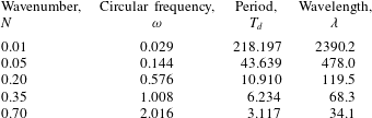
is 23.9. For reference, table 1 provides the range of
 $N$
used in this investigation and other corresponding disturbance parameters.
The disturbance parameters used in this study.

3 Static structure and single-pulse disturbance
3.1 Static structure with resolution study
The ODW in the steady inflow with
 $M_{0}=10$
and
 $\unicode[STIX]{x1D703}=30^{\circ }$
is first simulated as the basic structure. A Cartesian grid is used to discretize the rectangular domain, and the square grid
 $0.10\times 0.10$
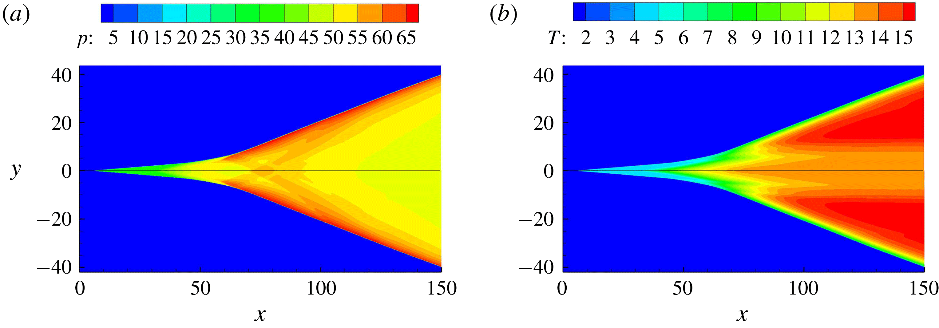
is used as the default grid. Equivalently, the default grid size corresponds to 10 points per CJ-ZND (Chapman–Jouguet/Zeldovich–von Neumann–Döring) induction zone length. Figure 2 first shows pressure and temperature with two different grid sizes for verification, illustrating a typical structure with smooth initiation transition. The initiation features a curved shock around
 $x=70$
, and the oblique angle increases obviously due to the heat release. This structure has been observed in our previous studies (e.g. Yang et al.
Reference Yang, Teng, Jiang and Ng2018, Reference Yang, Teng, Ng and Jiang2019). The chemical parameters of the present study, i.e.
 $Q=50$
and
 $\unicode[STIX]{x1D6FE}=1.2$
, have in fact been employed widely in earlier studies based on the one-step Arrhenius kinetic model. It gives a Mach number of CJ detonation
 $M_{CJ}$
equal to 6.22. For an inflow Mach number
 $M_{0}=10$
and wedge angle
 $\unicode[STIX]{x1D703}=30^{\circ }$
as chosen in this work, the overdriven degree
 $f$
of the resulting ODW is 1.47. For comparison, this overdriven value is close to that of the ODW in stoichiometric hydrogen–air mixtures with
 $M_{0}\approx 7.8$
, which has been simulated in our recent studies (Teng, Ng & Jiang Reference Teng, Ng and Jiang2017; Fang et al.
Reference Fang, Hu and Teng2018).
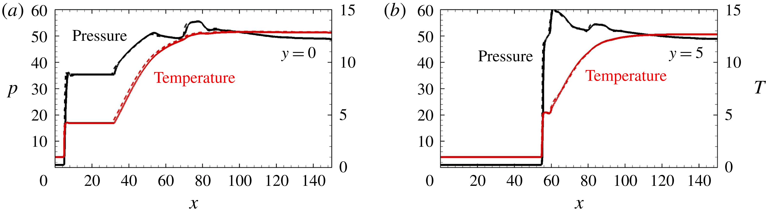
The effect of the grid is also assessed in figure 2. As shown, the flow fields are almost the same and the differences are hard to distinguish. To provide quantitative comparison, the pressure and temperature along the lines
 $y=0$
and 5 are shown in figure 3. Clearly, the curves are overlapped together so the effects of different grids are found to be negligible. Moreover, these curves show different coupling of shock and heat release along different lines. Along the wedge, i.e.
 $y=0$
, the shock is inert and uncoupled with the heat release, generating the long induction region. Conversely, along the initiation region, i.e.
 $y=5$
, the coupling of shock and heat release is generated but weak, resulting in the short induction region with a post-shock pressure rise. In the case of strong coupling on the oblique detonation surface, the pressure peak appears on the surface and then decays, different from that shown in figure 3.
Pressure (a) and temperature (b) of ODW with
 $M_{0}=10$
, grid
 $0.10\times 0.10$
(upper) and
 $0.05\times 0.05$
(lower).

Pressure and temperature along the lines
 $y=0$
(a) and 5 (b) with
 $M_{0}=10$
, grid
 $0.10\times 0.10$
(solid) and
 $0.05\times 0.05$
(dashed).

3.2 Single-pulse disturbance with low and modest
 $N$

Temperature of flow fields with single-pulse disturbance and
 $N=0.01$
.

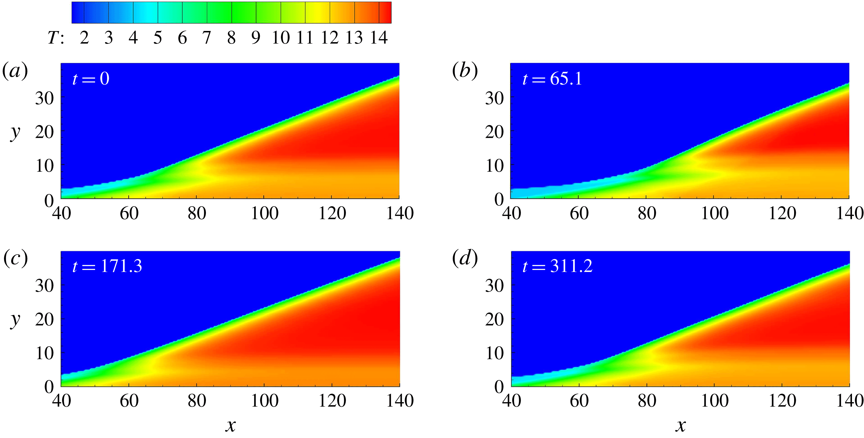
To analyse the ODW dynamics in an unsteady flow, the structure is first disturbed by a single pulse with
 $N=0.01$
, a rather low
 $N$
value corresponding to a slowly changing disturbance. As shown in figure 4, the ODW keeps almost the same wave structure, e.g. the transition by curved shock and the smooth oblique detonation surface, but its initiation region moves due to the imposed disturbance. From figure 4(a) to 4(b), it first moves downstream. The downstream movement of the ODW is due to the increase of density by the disturbance, i.e.
 $1+A\sin (\unicode[STIX]{x1D714}t)$
, in the first quarter cycle. Hence the temperature decreases, resulting in a reduction in the reaction rate. In the present simulations, the inflow velocity is fixed and hence the temperature variation also results in the increase of
 $M_{0}$
. Theoretically, increasing
 $M_{0}$
would accelerate the chemical reaction rate. Nevertheless, as determined from the numerical results, the decrease of temperature is found to be predominant for the reaction rate. After the downstream movement period, the density decreases (or temperature increases) below the average value, so the upstream movement of the ODW is observed in figure 4(c). Finally, the ODW moves back to the initiation position, as shown in figure 4(d). Because
 $N$
is very low, the structure evolution is quasi-steady without complicated phenomena observed. This result is similar to that in our previous study (Zhang et al.
Reference Zhang, Yang, Teng, Ng and Wen2018), where only an incremental abruptly changing disturbance is introduced.
Temperature of flow fields with single-pulse disturbance and
 $N=0.05$
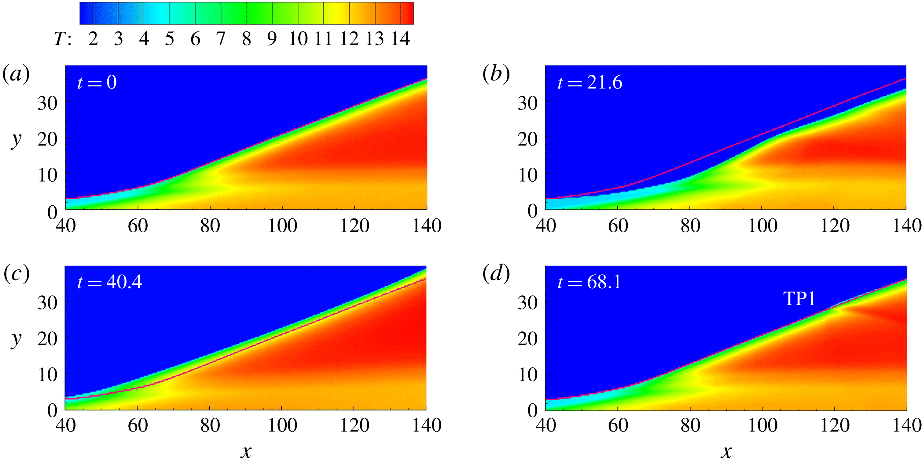
. (The red curve denotes the initial or steady shock position.)

Temperature of flow fields with an opposite single-pulse disturbance
 $1-A\sin (\unicode[STIX]{x1D714}t)$
and
 $N=0.05$
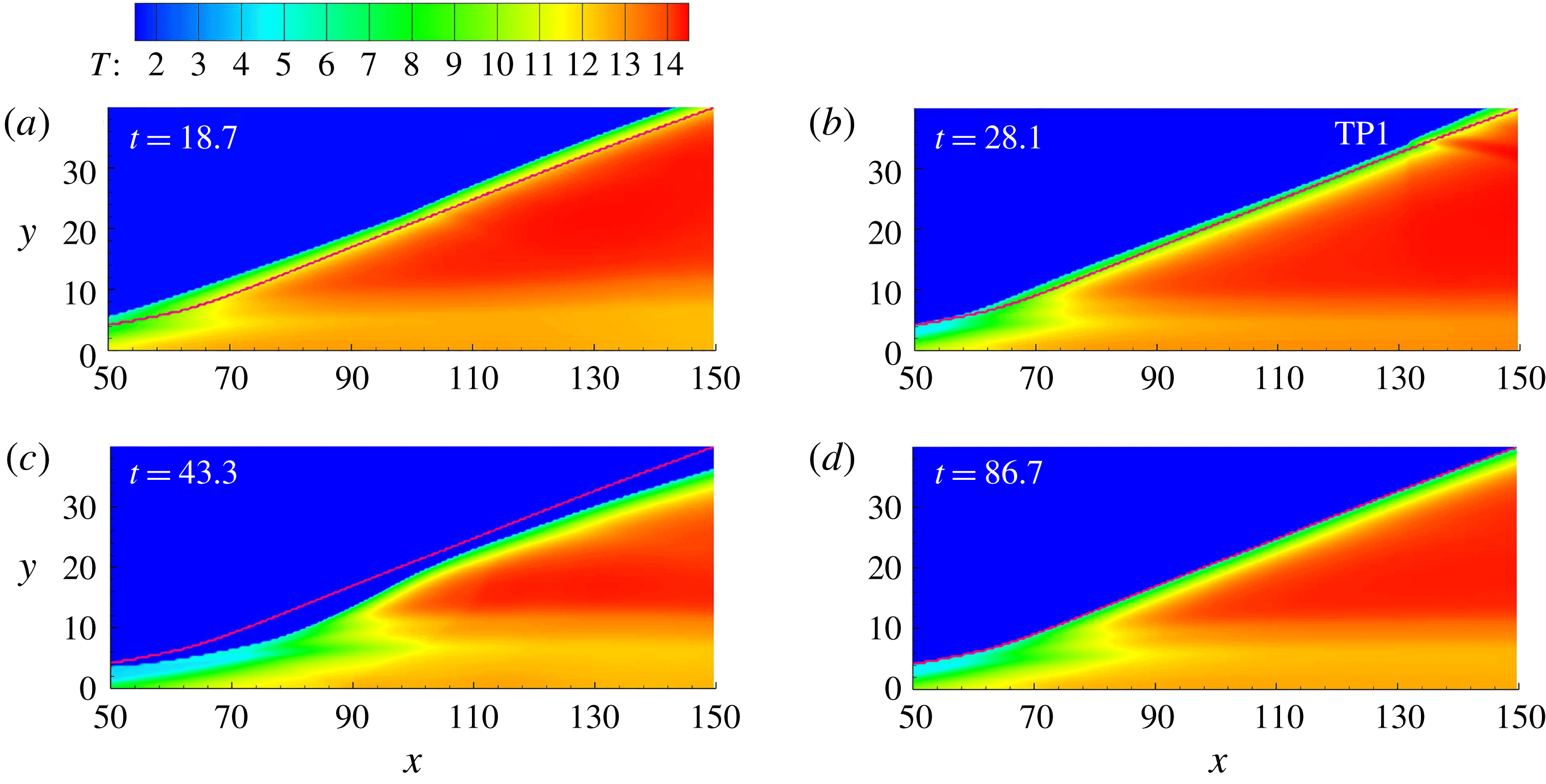
. (The red curve denotes the initial or steady shock position.)

The present simulation study demonstrates that increasing
 $N$
results in different evolution processes. With
 $N=0.05$
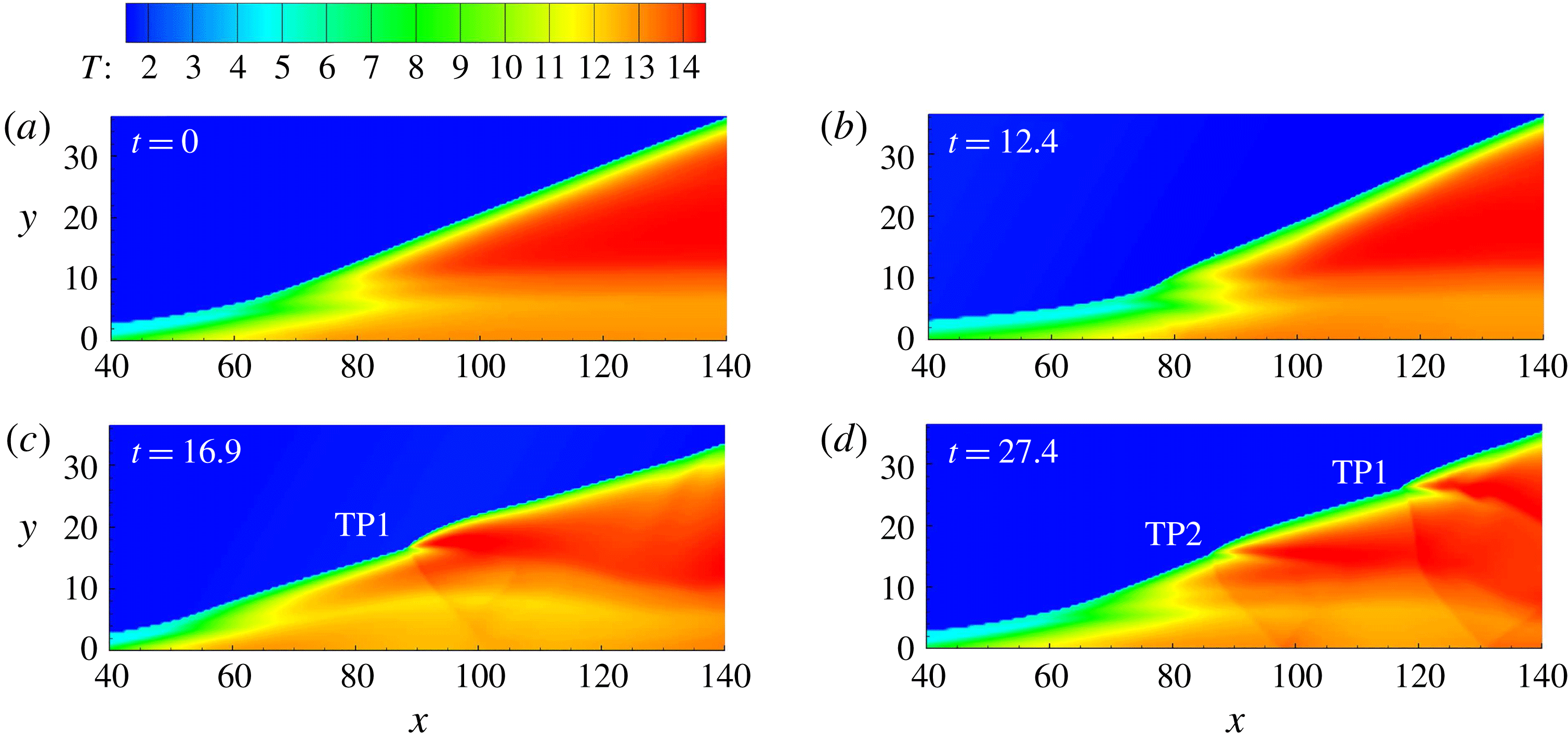
, as shown in figure 5, the structure moves downstream first, from figure 5(a) to 5(b), and then moves upstream in figure 5(c). Different from the previous case, the evolution induces the curved oblique detonation surface, and finally generates one triple point, as shown in figure 5(d). In this case, the triple point forms when the ODW moves from upstream position to its equilibrium position, at the fourth quarter cycle. To investigate the formation of the triple point, the opposite disturbance, i.e.
 $1-A\sin (\unicode[STIX]{x1D714}t)$
, is imposed. As shown in figure 6, the triple point also appears, but in the second quarter cycle rather than the fourth quarter cycle. Therefore, with a modest
 $N=0.05$
, the formation of one triple point, destabilizing the ODW surface, is unavoidable.


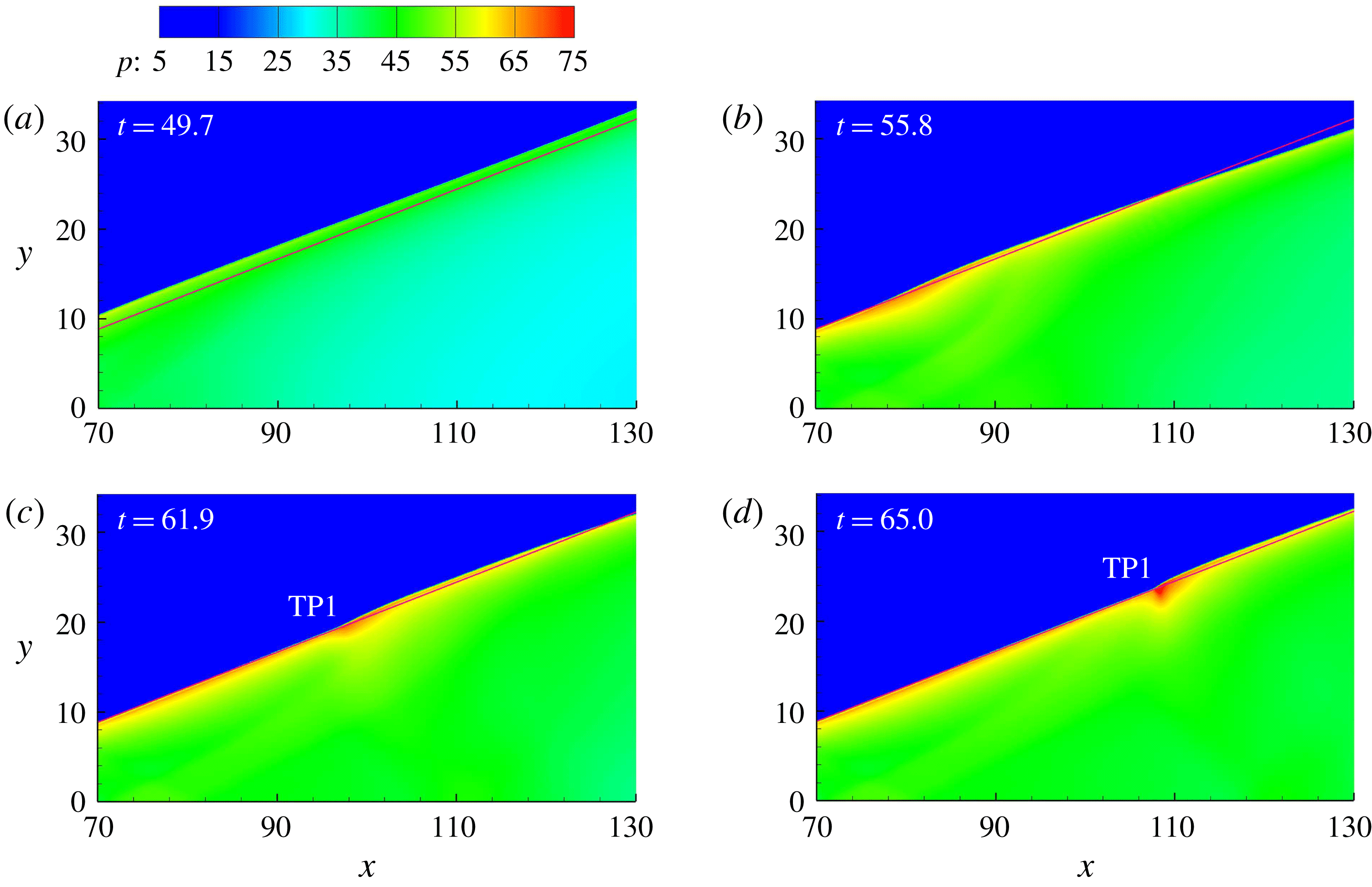
To clarify the formation mechanism of the triple point on the surface, the pressure fields of figure 5, i.e. single-pulse disturbance and
 $N=0.05$
, are displayed in figure 7. It can be observed that the surface is almost parallel with the initial shock in figure 7(a). However, when moving downstream, different parts of the surface have different velocities. Notably, the surface around
 $x=130$
even moves beyond its equilibrium position in figure 7(b). It induces a convex surface and subsequently a triple point forms gradually, as shown in figure 7(c,d). A similar process occurs in figure 6, because its second quarter cycle corresponds to the process when the surface moves from upstream to the equilibrium position.
Temperature fields with single-pulse disturbance and
 $N=0.20$
.

Further increasing the
 $N$
value to 0.20, a similar process is observed in figure 8. However, a more distorted wave surface is generated, with two triple points marked in figure 8(d). These results demonstrate that the evolution of the ODW is strongly dependent on
 $N$
. For all single-pulse cases, the resulting triple points induced by the inflow disturbance will be convected downstream, and the ODW surface returns to a smooth state when the disturbance is over.
Positions of reactive front along different lines with single pulse disturbance and
 $N=0.01$
, 0.05, 0.20 (
 $y=0$
, red; 5, green; 20, blue; 35, black).

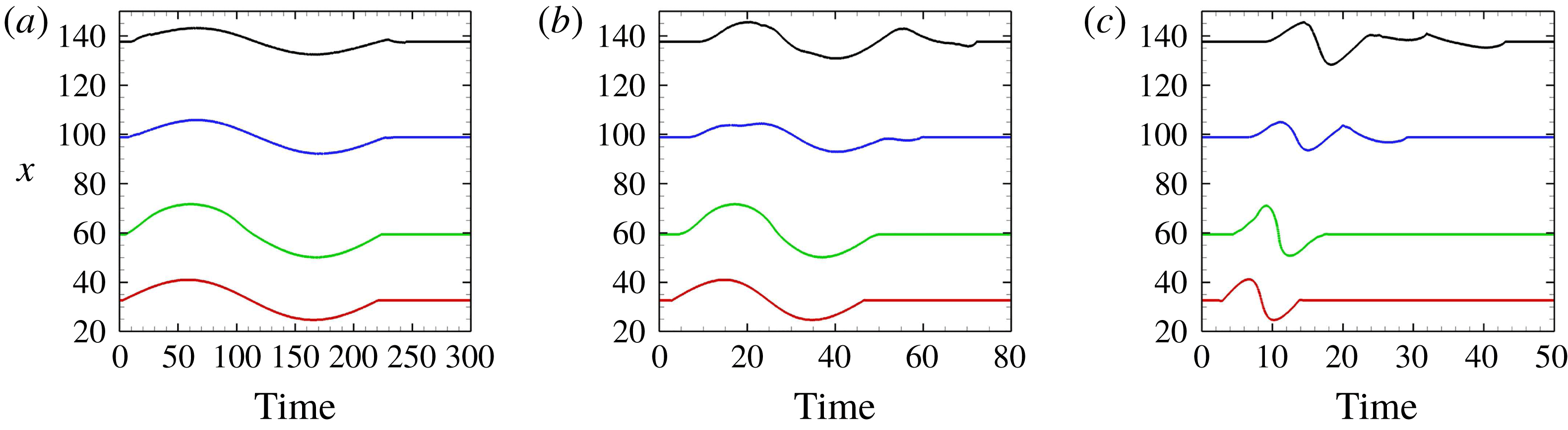
To demonstrate how the disturbed ODW evolves, the positions of the reactive front along different lines, parallel to the
 $x$
-axis, are plotted as a function of time. The reactive front location is defined by the end of the induction reaction where heat release begins, i.e.
 $\unicode[STIX]{x1D709}=0$
and
 $\unicode[STIX]{x1D702}=0$
. The results with
 $N=0.01$
, 0.05 and 0.20 are shown in figure 9. It is observed that the disturbance induces the reactive front to move downstream and upstream in all cases. However, the moving pattern depends significantly on
 $N$
. With
 $N=0.01$
, the disturbance is more spread and the ODW structure has more time to adjust and hence the flow field remains quasi-steady. The movement of the reactive front along different lines remains almost the same, except that the amplitude varies. By increasing
 $N$
, e.g. to
 $N=0.05$
, different locations along the ODW will experience the main effect of the pulse disturbance at different times. For instance, the downstream line, such as
 $y=35$
, has much longer time length than that along
 $y=0$
. Furthermore, the movement of the reactive front becomes irregular on the downstream surface. With
 $N=0.20$
, the ODW experiences a more abrupt perturbation and a more noticeable response in the initiation region begins to appear which persists downstream. An increasing phase shift also results from larger
 $N$
due to the significant time difference at which the downstream section experiences the disturbance at higher
 $N$
, and thus destabilizes the oblique detonation surface. The structure loses its stability with the flow and the disturbance thus causes primarily a distorted surface with fine unstable feature.
3.3 Single-pulse disturbance with high
$N$

Temperature of flow fields with single-pulse disturbance and
 $N=0.35$
.

Temperature of flow fields with single-pulse disturbance and
 $N=0.70$
.

Resolution study of the case with single-pulse disturbance and
 $N=0.35$
at
 $t=21.4$
, grid
 $0.10\times 0.10$
(upper) and
 $0.05\times 0.05$
(lower).

Increasing
 $N$
further to 0.35 and 0.70, more complicated results are observed, as shown in figures 10 and 11. Different from those with modest
 $N$
(e.g.
 $N=0.20$
), the movement in the initiation region becomes weak, but the surface is disturbed strongly, including the new shock/reaction front complex. With
 $N=0.35$
, besides the two triple points observed, another triple point RTP1 (reverse triple point 1) appears, which has different features from TP1 and TP2. As found in Teng et al. (Reference Teng, Ng, Li, Luo and Jiang2015), this triple point RTP1 and its connected transverse wave face downstream, rather than upstream like TP1 and TP2. With
 $N=0.70$
, two reverse triple points, RTP1 and RTP2, appear, demonstrating a more dynamic unstable surface. It should be noted that, in these cases, the ODW location remains almost the same, suggesting that the movement of the whole structure is absent in these cases. To verify if the generation and movement of these triple points are not influenced by the effect of the numerical grid, a resolution test is performed for the case of
 $N=0.35$
by comparing the results with the default grid size
 $0.10\times 0.10$
and half of it, i.e.
 $0.05\times 0.05$
. As can be seen in figure 12, there is hardly any difference between the simulation results obtained using the two grid resolutions.
Positions of reactive front along different lines with single-pulse disturbance and
 $N=0.35$
, 0.70 (
 $y=0$
, red; 5, green; 20, blue; 35, black).

The positions of the reactive front along different lines are also plotted for
 $N=0.35$
and 0.70 as a function of time in figure 13. The downstream perturbed time scale decreases but its ratio to the time length along the wedge increases. Along
 $y=0$
, the slowly increasing/rapidly decreasing profiles become obvious. This perhaps can be explained by the fast change in density with large
 $N$
and the exponential temperature sensitivity in Arrhenius kinetics. In addition, the displacement of the reactive front is weakened downstream, but displays irregular oscillations with small amplitude.
4 Structure evolution under multi-pulse disturbance
4.1 Multi-pulse disturbance with low and modest
$N$

Pressure fields with multi-pulse disturbance and
 $N=0.05$
.

The cases under the multi-pulse disturbance are simulated and discussed in this section. Numerical results demonstrate that, with
 $N=0.01$
, the movement of the ODW is almost the same as that shown in figure 4, so is not displayed here. This observation demonstrates that the interaction of different perturbation cycles is negligible, which should be attributed to the quasi-steadiness of the flow field derived from low
 $N$
. However, the similarity breaks down when
 $N$
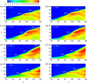
increases to 0.05, as shown in figure 14. According to table 1, a cycle takes the time interval of 43.639, and figure 14(a–d) shows the downstream movement, while figure 14(e–h) shows the upstream movement. A curved surface is generated by the disturbance like that in the single-pulse case, but no triple point forms, different from the single-pulse case shown in figure 5. Considering that the disturbances of both cases have totally the same characteristic parameters, the absence of a triple point should be attributed to the successive disturbance. In other words, the formation of a triple point is suppressed by the next disturbance cycle.
Temperature of flow fields with multi-pulse disturbance and
 $N=0.20$
.

Increasing
 $N$
to 0.20, the flow field becomes very complicated, and several triple points induce the periodic unstable surface. To analyse the evolution, figure 15 presents a whole cycle giving approximately the same first and last frames. In figure 15(a), two triple points, TP1 and TP2, appear connected with the downstream convex surfaces. When TP1 and TP2 move downstream, the upstream straight surface evolves, developing into two sections with a clear boundary. These two sections have different evolution processes, and another triple point TP3 appears on the boundary, as shown in figure 15(e). Consequently, three triple points move downstream, resulting in a flow field of figure 15(h). It eventually returns to be the same as that of figure 15(a), except that TP2 replaces TP1 and TP3 replaces TP2.
Compared with the case with the same
 $N=0.20$
but single-pulse disturbance shown in figure 8, the multi-pulse disturbance actually displays a more involved evolution of the ODW structure. Three triple points coexist on the surface, connected by convex and concave surfaces evolving periodically. Thus, the surface becomes more complicated than that in the single-pulse case, different from the cases with
 $N=0.05$
. However, it should be noted that there is only one triple point generated for each cycle in this case, while two triple points are generated in the corresponding single-pulse case. Hence, this is similar to the cases with
 $N=0.05$
, demonstrating that the formation of a triple point is indirectly suppressed by the next cycle.
Positions of the reactive front along different lines with multi-pulse disturbance and
 $N=0.01$
, 0.05, 0.20 (
 $y=0$
, red; 5, green; 20, blue; 35, black).

The positions of the reactive front along different lines are plotted, as shown in figure 16. With
 $N=0.01$
, the oscillations along different lines parallel to the
 $x$
-axis have almost the same profiles but different amplitudes. When the surface extends downstream, the amplitude first increases from the line
 $y=0$
to 5, due to more temperature sensitivity in the lower-temperature induction region, and then decreases after that in the ODW regime. In the cases of
 $N=0.05$
and 0.20, the distorted profiles, which deviate from the initial sinusoidal disturbance, are observed, and the deviation becomes intense in the
 $N=0.20$
case. It should be noted that, for each
 $N$
, oscillations along different lines have roughly the same cycle with the inflow disturbance, demonstrating that these are inflow-triggered oscillatory features rather than deriving from the inherent ODW instability.
Oscillation amplitude with multi-pulse disturbance and
 $N=0.01$
, 0.05, 0.20.

To quantify the oscillation pattern, the peak-to-peak amplitude variation is retrieved from the data and shown in figure 17. The basic case shown in the plot results from the static simulations with inflow density
 $1\pm 0.2$
, corresponding to the maximum disturbed inflow conditions. The amplitude of the base case is obtained according to the final reactive front positions for these two extreme perturbed conditions (i.e.
 $\unicode[STIX]{x1D70C}_{0}=0.8$
and 1.2). It is thus not a real oscillation, but provides a baseline to examine the reaction surface behaviour. The numerical results demonstrate that the oscillation amplitudes in the case of
 $N=0.01$
almost overlap with the basic results, confirming that the low
 $N$
induces only the quasi-steady flow fields. The oscillation amplitude is displayed by the increase–decrease curve for both the base and
 $N=0.01$
cases. It is interesting to note that, with the same sinusoidal inflow disturbance, the amplitude along
 $y=5$
has the maximum amplitude. This position corresponds to the initiation region, demonstrating that the initiation region is sensitive and prompt to oscillate under inflow disturbance. When the surface extends downstream, the amplitude decreases for both the base and
 $N=0.01$
cases.
However, the amplitude variation is different for the other two cases with
 $N=0.05$
and 0.20. As shown in figure 17, an obvious deviation of these two curves from that of
 $N=0.01$
appears when the surface extends downstream. On the line
 $y=15$
, the difference is approximately 1.0, which increases to approximately 2.5 on the line
 $y=20$
. Nevertheless, the difference does not increase further because the decrease of the amplitude with
 $N=0.05$
becomes slow from
 $y=20$
to 25. On the lines
 $y=30$
and 35, the amplitude of the case with
 $N=0.05$
is larger than that of the base case. In general, when
 $y$
increases from 0 to 30, the amplitude first becomes smaller than that of the base case, i.e. referred to as an undershooting oscillation, and then becomes larger than that of the base case, an overshooting oscillation. The latter is of interest since the overshoot, large-amplitude oscillation can induce a more prominent effect on the instability onset of the ODW. By increasing
 $N$
to 0.20, the phenomenon becomes significant and overshooting appears earlier. It can be observed that the undershooting–overshooting boundary moves from 25–30 to 15–20, and both the peak and trough of the curve become larger than those of the
 $N=0.05$
case.
4.2 Multi-pulse disturbance with high
$N$

Temperature fields with multi-pulse disturbance,
 $N=0.35$
.

Temperature fields with multi-pulse disturbance,
 $N=0.70$
.

In the single-pulse disturbance cases, further increasing
 $N$
above 0.20 introduces more triple points, including those reverse triple points facing downstream. In the multi-pulse disturbance cases, increasing
 $N$
results in similar phenomena, as shown in figures 18 and 19. With
 $N=0.35$
, there exist convex and concave surfaces connected by triple points, appearing as a cellular surface, and the ODW evolves and new triple points form periodically. With
 $N=0.70$
, the surface contains more triple points, and the length of the curved surface becomes short. Although the flow fields seem increasingly complicated, there exists a strict periodic evolution. The triple points are numbered in figures 18 and 19, demonstrating that, for one cycle, only one triple point forms in these two cases. In figure 19, RTP2 forms on the downstream surface, demonstrating that a new triple point may appear and induce more complicated local structures, but the flow fields stay the same after the time of one cycle.
Pressure (a) and temperature (b) fields with multi-pulse disturbance and
 $N=0.35$
, grid
 $0.10\times 0.10$
(upper) and
 $0.05\times 0.05$
(lower).

Resolution study of the case with multi-pulse disturbance and
 $N=0.35$
, grid
 $0.10\times 0.10$
(solid) and
 $0.05\times 0.05$
(dashed); (a) pressure and temperature along
 $y=0$
; (b) positions of reactive front along different lines.

To ensure that the numerical resolution is again sufficient in simulating these fine structures, the pressure and temperature fields of the case with
 $N=0.35$
are shown in figure 20. Decreasing the grid from
 $0.10\times 0.10$
to
 $0.05\times 0.05$
, it is again shown that the two wave structures are essentially the same. Further evidence includes the pressure and temperature curves along
 $y=0$
, in figure 21(a), and the positions of the reactive front along different lines, illustrating an oscillation in figure 21(b). All these results reconfirm that the grid
 $0.10\times 0.10$
is sufficient to provide results with enough detail to explore the ODW dynamics.
Positions of the reactive front along different lines with multi-pulse disturbance,
 $N=0.35$
(a) and 0.70 (b) (
 $y=0$
, red; 5, green; 20, blue; 35, black).

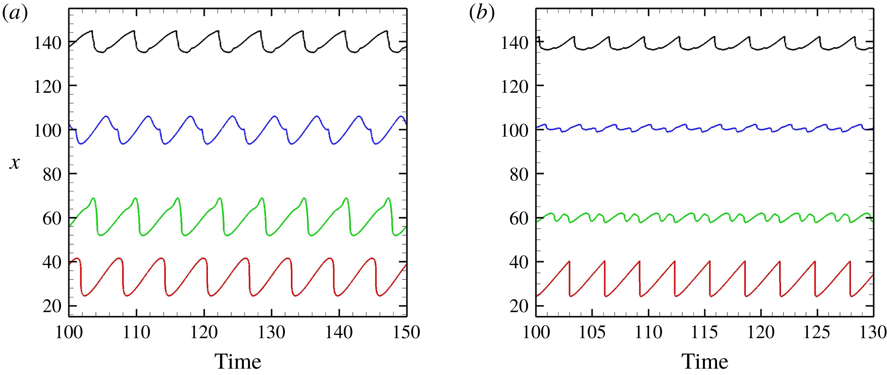
The positions of the reactive front along different lines with high
 $N$
are shown in figure 22. The oscillation is distorted more significantly when
 $N$
rises to 0.35 or 0.70, and the slowly increasing/rapidly decreasing profiles are observed on the line
 $y=0$
. The rapidly decreasing trend evolves into a jump in figure 22(b), which should be attributed to the formation of a new reactive zone. In the case of
 $N=0.70$
, the disturbance induces an isolated reactive zone in the induction region (see figure 19), and this high-temperature zone moves downstream and merges with the original reactive front. In the case of
 $N=0.35$
, the formation of a new reactive zone is hard to distinguish from flow fields (see figure 18); the process is similar, so a jump of reactive front position appears in figure 22(a).
To analyse the oscillation amplitude quantitatively, the amplitude curves with
 $N=0.35$
and 0.70 are shown in figure 23. It is observed that, in the case of
 $N=0.35$
, the amplitude reaches its minimum value quickly when
 $y=10$
. After that, the amplitude increases and stays almost the same as that in the base case. However, in the case of
 $N=0.70$
, the amplitude decreases to a very low value and remains there, with a very complicated cellular surface as shown in figure 19. In general, the inflow disturbances of these two cases lose the ability to oscillate the whole reaction structure, but instead develop local fine unstable features.
Oscillation amplitude with multi-pulse disturbance,
 $N=0.35$
(a) and 0.70 (b).

4.3 Discussion on the dynamic structure
Based on the simplest ODW formation structure with smooth initiation transition, inflow disturbances, modelled by the sinusoidal inflow density/temperature, are introduced and the effects of disturbance wavenumber
 $N$
are investigated in this study. Different from the static ODW in the steady inflow, the disturbance can induce complicated wave structures on the oblique detonation surface. The present investigation primarily focuses on the ODW evolution in unsteady flow by introducing a continuous disturbance. Oscillations of the reactive front as well as several new fine wave structures are observed. These are further analysed in the following to deepen the understanding of the unsteady ODWs.
Numbers of triple points derived from the disturbance (the second number with high
 $N$
denotes the number of reverse triple points, which face downstream).

To facilitate the analysis of the triple point formation, table 2 shows the number of triple points generated in one cycle. At first sight, this seems to contradict the direct observation of flow fields, because a multi-pulse disturbance appears to provide more triple points to the surface at certain instants. However, the results in table 2 demonstrate that, for each given
 $N$
, the triple point number of the multi-pulse case is no more than the number of the single-pulse case. It is not surprising that, in the case of
 $N=0.01$
, no triple point is generated, because the flow is quasi-steady. The two cases with
 $N=0.05$
and 0.20 are similar, showing that one or two triple points are generated in the case of a single-pulse disturbance, while no triple point for
 $N=0.05$
and only one triple point for
 $N=0.20$
in the case of a multi-pulse disturbance. These results demonstrate that the effects of a continuous disturbance weaken the ability to generate the triple points. Further increasing
 $N$
to 0.35 or 0.70 induces more triple points, but the trend remains the same, i.e. fewer triple points in multi-disturbance cases. The reverse triple points, which face downstream, are also generated in these cases. More triple points, including regular and reverse ones, are generated in the single-pulse cases, but at most one pair of triple points is generated in one cycle of multi-pulse cases.
The formation of triple points on the ODW surface is a topic that has been studied widely. However, the underlying mechanism derives primarily from the intrinsic instability discussed in most of previous studies (e.g. Papalexandris Reference Papalexandris2000; Choi et al. Reference Choi, Kim, Jeung, Ma and Yang2007; Teng et al. Reference Teng, Ng, Li, Luo and Jiang2015). Using the power spectral density (PSD) analysis, it is found that the small disturbance from the initiation region may facilitate the surface instability and accelerate the triple point formation in the case of low inflow Mach number (Yang et al. Reference Yang, Teng, Ng and Jiang2019). This work actually demonstrates a different situation, because the basic ODW in steady flow has a smooth surface. The triple points, which derive from the disturbance, disappear as shown in single-pulse cases. The intrinsic instability generates the triple points through the small disturbance, which is amplified gradually and usually a section of smooth surface can be observed (e.g. Choi et al. Reference Choi, Kim, Jeung, Ma and Yang2007; Yang et al. Reference Yang, Teng, Ng and Jiang2019). In this study, the triple points are generated through an embedded disturbance from the inflow, and close to the initiation region. However, the unstable surfaces featured by several triple points can be observed in the cases of continuous disturbance, giving rise to similar fine structures. Furthermore, the reverse triple points form at the rear side of regular triple points and amplified while convecting downstream. This formation is similar to that of our previous study (Teng et al. Reference Teng, Ng, Li, Luo and Jiang2015).
The other aspect that deserves more attention is the oscillation of the reactive front position. The movement of the reactive front has also been mentioned in a few other studies (e.g. Liu et al.
Reference Liu, Wu, Yao and Wang2015; Zhang et al.
Reference Zhang, Yang, Teng, Ng and Wen2018), while the oscillation around a certain position has only been observed in our very recent study (Yang et al.
Reference Yang, Teng, Jiang and Ng2018). The latter occurs in a steady inflow and derives from the low inflow Mach number, different from the presently observed oscillation, which occurs in an unsteady flow. It is found that the wavenumber
 $N$
plays a critical role in the unsteady ODW behaviour, and three regimes can be distinguished from the above results, referred to as the quasi-steady, overshooting oscillation and unstable surface. The quasi-steady one corresponds to low
 $N$
, and the effects of the next cycle can be neglected. The regime of overshooting oscillation corresponds to modest
 $N$
, typified by the amplified movement of downstream reaction surface. The unstable surface corresponds to high
 $N$
, and the initiation region is disturbed significantly. It is of interest to examine and compare with the oscillation amplitude, or movement amplitude in single-pulse cases. Besides its dependence on
 $N$
, the amplitude also changes along different lines parallel to the
 $x$
-axis. However, this variation retains similar trends in the cases of both single-pulse and multi-pulse disturbances. For example, the amplitude follows the increasing–decreasing–increasing variation, as shown in figures 9(c) and 16(c). This demonstrates that the amplitude variation is not derived solely from the continuous disturbance, although it has not been clarified before.
The overshooting oscillation, i.e. large-amplitude oscillation of a certain downstream surface, appearing in modest
 $N$
cases, is an intriguing phenomenon never reported before. A previous study (Zhang et al.
Reference Zhang, Yang, Teng, Ng and Wen2018) indicates a slight overshooting when the ODW moves downstream induced by decreasing wedge angle. When arriving at the equilibrium position, the structure does not stop but continues to move further downstream, and then returns to its equilibrium position from downstream. However, this dynamics occurs in steady flow and the overshooting range is weak. To investigate the overshooting, more cases are simulated and the amplitude along the line
 $y=35$
is plotted as a function of
 $N$
; see figure 24. The case
 $N=0.01$
provides a baseline, with an amplitude of approximately 11, and the overshooting can be observed clearly for
 $N<0.3$
. Further increasing
 $N$
above 0.35, the overshooting disappears. At high
 $N=0.70$
, local unstable features develop and the effect of inflow disturbance is spread along the ODW surface. Although the ODW appears unstable or cellular, it becomes more robust, resulting in smaller reaction front amplitude fluctuation. This is equivalent to the results by Gamezo, Desbordes & Oran (Reference Gamezo, Desbordes and Oran1999), which show that the overall dynamics of a normal, unstable cellular detonation is robust to small heat release perturbations. The overshooting also appears in the cases of single-pulse disturbance, even stronger, and a minimum amplitude appears around 0.45. The overshooting oscillation can be viewed as the flow-determined disturbance, i.e. the reaction front displacement is sensitive and primarily controlled by the inflow disturbance. From the viewpoint of disturbance frequency or wavenumber, this overshooting reflects a resonance-like behaviour. The maximum amplitude of oscillation appears with a modest
 $N$
, suggesting a strong close coupling or phasing between the unsteady flow–heat release and onset of the triple point formation. This is a qualitative analysis, and further detailed study is necessary in the future.
Wavenumber
 $N$
versus amplitude along
 $y=35$
, for both single-pulse and multi-pulse cases.

5 Conclusions
The concept of an ODW engine has the potential for aerospace propulsion applications, and hence its dynamics in unsteady flow needs to be clarified. Any perturbation of the inflow parameters may induce the movement of ODW initiation position, and affect the formation structure and the subsequent ODW evolution. As a first step, this study models the unsteady inflow by a continuous sinusoidal density/temperature disturbance, and the ODW dynamics are simulated and discussed.
Based on a typical initiation structure with smooth transition with a curved shock, this study simulates ODWs subject to single-pulse and multi-pulse disturbance imposed in the inflow. By varying the wavenumber
 $N$
of the disturbance, increasing complexity of the ODW structure and dynamics are observed and analysed, including the triple point formation and oscillation of the reactive front. More triple points, including regular and reverse ones, are generated in the single-pulse cases, but at most one pair of triple points is generated in one cycle of multi-pulse cases. These results demonstrate that indeed the effects of continuous disturbance weaken the ability to generate the triple points.
The oscillation or movement of the reaction front is plotted and analysed for both the single-pulse and multi-pulse cases. Generally, it is found that low
 $N$
induces the quasi-steady flow fields, and the oscillation amplitudes increase around the initiation region and then decrease downstream. With modest
 $N$
, the oscillation is undershooting near the initiation region but becomes overshooting downstream. The possible mechanism for these behaviours is mainly due to the unsteadiness, finite disturbance/response time scale, coherent phasing of the heat release with the disturbance and the onset of triple point formation. The overshooting phenomenon is found to be dependent on
 $N$
. Increasing
 $N$
above 0.35, the downstream overshooting disappears (i.e. with large peak-to-peak oscillation amplitude), indicating that a proper disturbance wavenumber
 $N$
is critical to generate the oscillation. The latter also indicates that the resulting ODW surface readjusts itself, with local unstable features becoming more robust, and the reactive front of the final unstable ODW structure is less susceptible to flow disturbance.
Finally, apart from the complicated wave dynamics illustrated and discussed in this paper, still more work is needed to clarify the ODW characteristics in unsteady flow and, further, its application for practical purpose. For instance, the basic structure is chosen here to be a typical ODW structure with smooth transition, and the disturbance amplitude is limited to 0.2, i.e. 20 % of the initial density. For future investigation, the other type of ODW structure, with abrupt transition, should be studied to explore the effects of different initiation structures subjected to unsteadiness. Different disturbance amplitudes can be considered in such a study to possibly reveal new interesting phenomena. Moreover, this study, as the first step, employs a structure without an intrinsically unstable surface due to its inherent instability. Future work should also consider the ODW with both inherent natural instability (i.e. using mixtures with higher temperature sensitivity) and outside disturbance, which may be necessary and critical in any application.
Acknowledgements
The research is supported by the National Natural Science Foundation of China NSFC (nos 11822202 and 91641130) and the Natural Sciences and Engineering Research Council of Canada NSERC (no. RGPIN-2017-06698).