


1 Introduction
The minimum capital requirement for banks set by the first accord of the Basel Committee on Banking Supervision in 1988 primarily focused on the credit risk of banks (Basel, 1988). In 1997 the agreement was amended to incorporate market risk for capital calculations (Basel, 1996). Since then much research has been done on measuring and managing market and credit risk for banks but very little attention has been given to other types of risk such as operational risk. However, large scale operational loss events such as the unauthorized trading at Barings Bank in the UK which led to its collapse in 1995, the $2.2 billion loss at National Australia bank in 2001 due to product issues and model errors in their HomeSide mortgage servicing subsidiary, the $2.2 billion settlement with investors of Enron in 2005 by JP Morgan Chase for their role in helping the failed energy company to provide misleading financial results, and more recently, the $7.2 billion loss due to fraudulent trading at Société Générale have made both industry and regulators realise that merely focusing on credit and market risk is insufficient to ensure the solvency of a bank. It has been found that operational risk in a bank is often much larger than the market risk (De Fontnouvelle et al., Reference De Fontnouvelle, Dejesus-Rueff, Jordan and Rosengren2006). In response, the Basel committee included operational risk as one of the risks that need to be quantified in their Basel II accord in 2004 (Basel, 2006).
However, there are definite challenges for risk managers in quantifying operational risk. Firstly, there is no widely accepted methodology to quantify operational risk. Secondly, the heavy-tailed nature of the operational loss distributions makes it difficult to estimate the tails, especially when data is inadequate. Thirdly, most of the Low-frequency/high-severity (LF/HS) operational losses are high degree unique events, which makes it even more difficult to model the tail. Given these circumstances the amount of unknown and the unknowable is far greater than the known in the area of operational risk. As a result there are considerable uncertainties regarding the economic capital estimates for operational risk. For example, using bank-level data of six large internationally active banks, De Fontnouvelle et al. (Reference De Fontnouvelle, Rosengren and Jordan2007) report a wide variation in the shape parameter (a low of 0.498 to a high of 0.859) of the fitted Generalized Pareto distribution (GPD) for the losses from each bank. In a comment on their paper Kuritzkes points out that this wide variation has a significant impact on the capital charge for individual banks. Using six hypothetical banks with identical exposures, Kuritzkes demonstrates that the capital charge can vary from $208 mill (if the shape parameter is 0.498) to $4,320 mill (if the shape parameter is 0.859). This significant variation raises the important question as to what extent banks and regulators can rely on bank level data to model the shape of the tail of the loss distribution. Given that banks are required to hold enough capital to cover one in a thousand year adverse event, it is obvious that it is impossible to observe the relevant operational loss data for capital estimation within any one firm. As a solution to this Basel II requires banks to use external data to complement their internal data. However, the process of combining internal data with external data is an exercise which requires due diligence due to biases inherent in the external data. If not properly combined, external data may distort parameter estimates and eventually lead to perverse estimates of economic capital (Baud et al., Reference Baud, Frachot and Roncalli2002). Wilson (Reference Wilson2007) points out there are three types of biases inherent to external data which may lead to poor estimates:
i) Reporting bias – occurs when different thresholds have been used by institutions to report losses to the external database
ii) Control bias – occurs when data is collected from institutions with different risk control systems
iii) Scale bias – occurs when data is collected from institutions with different sizes
In this paper we demonstrate how an external database can be used to model the severity of operational losses by correcting for reporting bias and scale bias.
The severity model developed in this study makes use of a method based on Extreme value theory proposed by De Fontnouvelle et al. (Reference De Fontnouvelle, Dejesus-Rueff, Jordan and Rosengren2006) to account for the reporting bias of the external data, and a regression analysis based on the GAMLSS framework introduced by Rigby & Stasinopoulos (Reference Rigby and Stasinopoulos2001, Reference Rigby and Stasinopoulos2005) to model the scaling properties of operational losses. The model can simulate losses for a bank given the size of the bank and other explanatory variables that might affect the severity of operational losses. The model is calibrated using the industry data and therefore can be used by banks with very little data of their own or by banks whose operational environment has changed significantly due to a merger or an acquisition. The next section provides a brief review of scaling models reported in the literature. The section 3 formulates the model and provides details of the research methodology, section 4 presents the results of the model after fitting it to data from the US banking industry, section 5 provides a demonstration of the severity model at work by computing capital estimates for several hypothetical banks as well as for two real banks by making simplified assumptions about the frequency distribution, and section 6 concludes.
2 Literature Review
It is natural to hypothesise that the severity of operational losses will have a relationship to the size of the bank. To the best of our knowledge, the first to test this hypothesis for financial firms were Shih et al. (Reference Shih, Khan and Medapa2000). They tested the correlation of the firm size indicators of revenue, assets, and the number of employees with the operational loss severities using the OpVar database (which is an external database consisting of publicly reported losses). They reported all three variables to be correlated with loss severity, with the revenue showing the strongest relationship. Furthermore, authors found that the relationship between the loss severity and the size of the firm is nonlinear. They reported that “a firm that is twice as large as another does not, on average, suffer a loss that is twice the size of the loss experienced by the other firm”. They hypothesised that the relationship between the loss severity and the size of a firm can be modelled as
 $$log(Los{{s}_i})\: = \:{{\beta }_0}\: + \:{{\beta }_1}\log (revenu{{e}_i})$$
An ordinary least squares (OLS) regression of the model confirmed a linear relationship between the log-loss severity and the log-revenue. However, authors reported the presence of heteroskedacity in the error term and corrected for this by running a weighted least squares (WLS) regression. They reported an adjusted R2 value of 9% for their WLS regression and concluded that the size only accounts for around 5% of the variability in the loss severity. Furthermore, they reported that “there is clear evidence of diminishing relationship between the size of a firm and loss magnitude”. A major limitation of this study is that authors did not correct for reporting bias in the external data. Later, De Fontnouvelle et al. (Reference De Fontnouvelle, Dejesus-Rueff, Jordan and Rosengren2006) showed that reporting bias in the OpVar database is too significant to be ignored. Therefore the results of the study should be taken with a grain of salt since parameter estimates are likely to be distorted as the model has been fitted using a disproportionate number of large losses.
Another early study to consider the scaling problem is Na et al. (Reference Na, Van Den Berg, Miranda and Leipoldt2006). Their study mainly analysed the scaling of aggregate losses as opposed to individual losses. Authors assumed aggregate operational losses can be broken down into two components, firstly a common component, which is assumed to be stochastic, capturing the influence on the loss severity by factors such as macroeconomic, geopolitical, cultural and business environment common to all banks and secondly an idiosyncratic component, which is deterministic, capturing the influence of the size of the bank on the loss severity. Their analysis revealed that the mean and the standard deviation of the aggregate losses scale similarly. Moreover, they found that the ratio of aggregate loss between two business lines (or banks) is simply equal to the ratio between their gross income. Authors also briefly analyzed whether their scaling model can be applied to individual loss severities. However, they reported that the results did not turn out to be convincing.
A study which took a slightly different approach to analyze the scaling properties of operational losses is that of Cope & Labbi (Reference Cope and Labbi2008). The authors used quantile regression techniques to analyse the relationship between different quantiles of the operational loss distribution and the size of a bank. Their study revealed that large losses scale differently from small losses and also confirmed a diminishing relationship between the loss size and the firm size for certain categories of operational losses. An important finding of their study is that not all operational losses are positively correlated with the size of a bank. They reported that for certain lines of business and event types, operational loss severity may decrease as the size of a bank increases. A limitation of the study is that in order to apply the quantile regression techniques proposed by the authors one needs to be able to identify the corresponding percentile level of each loss. However, it is not possible to achieve this when data is collected from more than one bank subject to a reporting threshold. To overcome this issue authors proposed a novel quantile matching algorithm. The algorithm requires the loss reporting threshold to be known and fixed. For some databases such as the ORX database, which the authors used in their study, this is not a problem. However, for most other external databases the loss reporting threshold of individual banks is unknown. In such instances one would require different techniques or a modification to the authors’ quantile matching algorithm.
A more recent paper to look at the scaling problem is by Dahen & Dionne (Reference Dahen and Dionne2010). They extended the work of Shih et al. (Reference Shih, Khan and Medapa2000) by introducing scaling factors other than the firm size into the regression analysis. Also, in contrast to Shih et al. (Reference Shih, Khan and Medapa2000) the authors used the Heckman method to correct for selection bias in the external data. The form of the regression model they employed is
 $$log(Los{{s}_i})\: = \:{{\beta }_0}\: + \:{{\beta }_1}\log (asset{{s}_i})\: + \:\mathop{\sum}\limits_{all\,j} {{{\beta }_j}B{{L}_{ij}}} \: + \:\mathop{\sum}\limits_{all\,k} {{{\beta }_k}E{{T}_{ik}}\: + \:{{e}_i}} $$
where, BLij is a business line indicator, ETik is an operational loss event type indicator, ei is an error term assumed to be normal, and βs are the parameters to be estimated. The model was fitted using OLS and an adjusted R 2 value of 29.58% was reported as an overall fit to the data. Although the value of R 2 is low, it was a significant improvement on the R 2 value reported by Shih et al. (Reference Shih, Khan and Medapa2000). However, given the low value of R 2 it is reasonable to question the appropriateness of the distributional assumption made by the authors that log-losses are Normally distributed. If the log-losses are distributed as a Normal distribution, then the losses should follow a Lognormal distribution. Although Lognormal distribution is a fairly heavy-tailed distribution, it is not as heavy-tailed as Pareto or Log-gamma distribution. Various previous studies have found evidence that operational losses are (extremely) heavy-tailed (see e.g., De Fontnouvelle et al., Reference De Fontnouvelle, Rosengren and Jordan2007; Moscadelli, Reference Moscadelli2004). The low value of the adjusted R 2 found by Dahen & Dionne (Reference Dahen and Dionne2010) could be possibly explained by the inappropriateness of the distributional assumption.
Another interesting study of the scaling problem is found in Wei (Reference Wei2007) where he tested the suitability of using the peak over threshold (POT) method from extreme value theory over the traditional actuarial techniques to model severity of losses. The author reported that the capital charge based on the Generalized Pareto distribution from the POT method was too conservative and too costly for the banks, whereas traditional actuarial models which assume losses arise from a known parametric family of distribution with scale parameter related to bank assets, provided a much more reasonable yet conservative capital estimates.
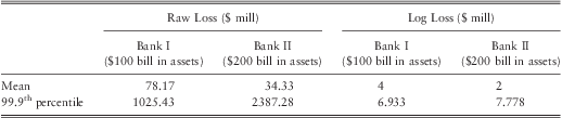
As discussed so far most of the previous work has focused on how the mean of the log-loss severity may scale in response to the size of a bank. However, there are several issues in this approach. Firstly, mean of the log-losses does not relate to any meaningful statistic of the (raw) loss distribution. Hence, results are difficult to interpret in most circumstances. Secondly, the operational risk capital charge for a bank is determined by the 99.9th percentile of the loss distribution. The information provided by a scaling model fitted to the mean of the log-losses provides very little information on how the 99th percentile may scale. To illustrate this point consider two banks denoted as Bank I and Bank II with assets of $100 bill and $200 bill respectively. Let's assume that the operational loss distribution of both banks follows a Log-gamma distribution with parameter values for Bank I being αI = 6.25, and pI = 25, and parameter values for Bank II being αII = 1.3889, and pII = 2.778 (the density function and a discussion of Log-gamma distribution will be given later in subsection 4.3.1). The mean and the 99.9th percentile loss for each bank under these distributional assumptions are given in table 1. One can observe from the table that the mean operational loss (as well as the mean log-loss) at the larger bank is less than half the mean loss at the smaller bank. However, the 99.9th percentile loss in the large bank is more than twice the loss in the small bank. In this particular example, the mean of the log-losses (as well as the mean of the raw-losses) and the 99.9th percentile of the log-losses scale in the opposite direction. In this situation OLS regression techniques (which have been used by many of the previous studies) would lead to a misleading conclusion that the size of a bank is negatively related to the loss severity. Although this may in fact be true of the mean of the loss distribution, in terms of capital calculation the result will be misleading.
Mean and the 99.9th percentile loss for the hypothetical Bank I and Bank II.
In general, mean of a loss distribution provides very little information when losses are heavy-tailed. Rootzén & Klüppelberg (Reference Rootzén and Klüppelberg1999) points out that “for catastrophic risk means don't mean anything”. To illustrate this we shall provide two slightly altered examples taken from their paper.
Consider that a bank is exposed to two types of risk. Under Risk Type I a bank may lose 1 with a probability of 50% or lose 1.5 with a probability of 50% for each day of 365 days. In contrast, under Risk Type II a bank may lose 0.2 with a probability of 99.85% or lose 700.2 with a probability of 0.15% for each day of 365 days. In this example the expected loss for both risk types is 456.25. However, the distribution of losses is quite different for the two types of risk, as illustrated in figure 1. One can observe that the mean is an important summary statistic for Risk Type I. However, for Risk Type II, mean has little significance in explaining the overall risk. Under risk type II, a bank may lose 73 with a probability of 58% or lose at least 773 with a probability of 42%. Clearly the second risk type is more risky than the first, but mean alone cannot differentiate this.
The distribution of total Losses for two risk types with same mean.

The second issue Rootzén & Klüppelberg (Reference Rootzén and Klüppelberg1999) raised is that mean may be quite unstable for losses which follow a heavy-tailed distribution. To illustrate this, consider two banks, Bank I and Bank II, in which operational risk follows a Pareto distribution; Pr(X > x) = x −α, for x > 1 with α = 1.01 for bank I and α = 1.001 for bank II. Figure 2 provides the plots of the density function of the loss distribution for the two banks. Clearly, both distributions are very similar. In fact, the loss level at the 99.9% percentile is 933 for Bank I and 993 for Bank II. Hence, the capital amount that the two banks need to hold should be very similar. However, the mean operational loss at Bank I is 101, whereas the mean loss at Bank II is 1001. The means differ by about a factor of 10. Again, this particular example demonstrates how the mean may be misleading for heavy-tailed risks. If one analysed the mean of the loss distribution of each bank, to find a relationship between the size of a bank and the severity of losses, the results could be misleading. In this instance considering the logarithm of losses will be useful. But as we demonstrated earlier, mean of log-losses does not necessarily need to follow the same scaling mechanism as the tail of the distribution. Hence, different techniques need to be considered.
The density of two different Pareto risks.

The preceding three examples illustrated why it is inappropriate to scale the severity of losses by using regression techniques which only try to fit the mean of the response variable. Such models may lead to spurious results about the relationship between the size of a firm and the loss severity even under correct distributional assumptions. A better approach to analyse the scaling properties would be to model the tail index of the loss distribution. In this study we explicitly model the tail index of the loss distribution by using size and other explanatory variables. We considered several distributional assumptions for operational loss data and found that a Log-gamma distribution provides the best fit. Our results suggest that the tail index of the operational loss distribution and the size of a bank have a negative relationship. In other words, the tail of the operational loss distribution in large banks is heavier than in small banks. In particular, we find that the 99th percentile loss can increase by up to 25% to 35% when the size of a bank doubles. Hence, our results suggest that the size of a bank has a more significant impact on the capital requirement than thought previously.
3 The Methodology
As discussed earlier, previous literature has revealed evidence of heteroskedacity in operational loss data. A one possible explanation for this could be the level of sophistication in banking activities between small banks and large banks. Small banks tend to carry out less sophisticated standard banking activities such as taking deposits, providing personal loans and facilitating transactions. The severity of operational losses which can arise from such activities tends to be lower. In contrast, in addition to standard banking activities, larger banks engage in more sophisticated banking activities such as securitization, trading of exotic securities, providing syndicated loans, assisting in mergers and acquisitions, and market making. The severity of operational losses from such complex banking activities is usually higher than those losses which can arise from standard banking activities. Since large banks engage in both standard as well as complex banking activities, it is reasonable to hypothesise that the variation in the severity of operational losses in a large bank is higher than in a small bank. Hence, a scaling model for operational losses should be able to account for this variation.
Furthermore, another issue which needs to be considered when developing a scaling model is the differences in severities across different operational risk events and business lines. The loss collection exercise by the Basel Committee in 2002 and 2008 has revealed that certain operational loss events and business lines have distributions with longer tails than the others (Basel, 2003; 2009). Hence, a model which only accounts for the variation in the mean of the severities for different categories of operational risk would not be able to capture the tail behaviour properly. In other words a good scaling model should be able to account for the variation in location, scale and shape of the distribution across different business lines and event types.
A convenient framework to model location, scale and shape of a distribution is the recently introduced ‘generalized additive models for location scale and shape’ (GAMLSS) (Rigby & Stasinopoulos, Reference Rigby and Stasinopoulos2001; Reference Rigby and Stasinopoulos2005). GAMLSS is a very general class of regression model that incorporates popular GLMFootnote 1, GAMFootnote 2, GLMMFootnote 3 and GAMMFootnote 4 together. However, GAMLSS is more general than the above mentioned, since firstly it relaxes the assumption that the response variable belongs to the natural exponential family. Hence, GAMLSS is a convenient framework to test various distributional assumptions such as Gumbel, Weibull and Student-t, in addition to the standard natural exponential family distributions.
The second advantage of the GAMLSS framework is that it does not limit the modelling to the location of the distribution as in GLM and the other similar frameworks. The standard GLM setup (similarly OLS) cannot model distributional parameters other than the location parameter explicitly by using explanatory variables. The ability of the GAMLSS framework to model all the distributional parameters allows one to estimate models with more flexible scaling properties. For example, if we assume log losses are distributed normally and if we model the standard deviation using the size of the bank as an explanatory variable, we can obtain a model that allows losses in a large bank to have a larger standard deviation compared to the losses in a smaller bank, but with both banks having the same mean (and median) logarithm of loss. In other words we can implicitly allow different quantiles of the distribution to scale differently. On the other hand, if we assume losses follow a Weibull distribution with shape parameter related to some covariates, then we could obtain a model which allows loss distribution to have either negative, positive or symmetric skewness depending on the values of the covariates.
In the GAMLSS framework all distributional parameters can be explicitly modelled using both fixed and random effects (Rigby & Stasinopoulos, Reference Rigby and Stasinopoulos2005). Furthermore, each distributional parameter can be modelled as linear and/or non-linear, parametric and/or smooth non-parametric functions of explanatory variables and/or random effects. In this study we limit our analysis to parametric linear GAMLSS models.
3.1 The Parametric Linear GAMLSS Framework
Consider log losses y = (y 1, y 2, …, yn)T are a random sample of independent observations. Let  $f({{y}_i};{{\bivartheta }_\iota })$ be the density function conditional on the parameter vector
 ${\bivartheta }_\iota}$. The
 ${\bivartheta }_\iota}$ can have any number of distributional parameters each of which can be modelled by explanatory variables. However, for the sake of simplicity in notation for the following discussion we shall assume
 ${\bivartheta }_\iota}$= (μi, σi)T is a vector of two distributional parameters.
We define a set of link functions that specifies the relationship between the linear predictor and the distributional parameters of each component distribution as
 $$\left \matrix { {{g}_1}({{\mu }_i})\: = \:{{\eta }_{i1}}\: = \:{{\beta }_{11}}\: + \:{{\beta }_{12}}{{X}_{i12}}\: + \:{{\beta }_{13}}{{X}_{i13}}\: + \: \cdots \: + \:{{\beta }_{1p}}{{\ X}_{i1P}} \cr\ {{g}_2}({{\sigma }_i})\: = \:{{\eta }_{i2}}\: = \:{{\beta }_{21}}\: + \:{{\beta }_{22}}{{X}_{i22}}\: + \:{{\beta }_{23}}{{X}_{i23}}\: + \: \cdots \: + \:{{\beta }_{2p}}{{X}_{i2P}}} \end{} \right\}i\: = \:1,\, \cdots \,,\,n,$$
where, Xijp is the value of the p th explanatory variable relating to the observation yi in the j th distributional parameter, and βjp is the parameter corresponding to Xijp. This set of equations can be simplified with the help of matrix notation as
 $$\matrix {{{g}_1}({{\bimu }_i})\: = \:{{\bi X}_1}{{\bibeta }_1} \cr\ {{g}_2}({{\bisigma }_i})\: = \:{{\bi X}_2}{{\bibeta }_2} \\ \end{}$$
where, Xj are the design matrix of the j th distributional parameter, and βj are the corresponding parameter vectors.
The maximum likelihood estimates of β1 and β2 can be obtained by solving
 $${\mathop{{{\rm{Max}}}}\limits_{{{{\bibeta }_1},\,{{\bibeta }_2}}}} \mathop{\sum}\limits_{i\: = \:1}^n {\log f({{y}_i};{{\bibeta }_1},\,{{\bibeta }_2})} $$
The optimization of eq. (1) can be carried out using the RS algorithm of Rigby and Stasinopoulos (Reference Rigby and Stasinopoulos2010, p. 92). We used the packages gamlss (Stasinopoulos & Rigby, Reference Stasinopoulos and Rigby2007) in software R (R Development Core Team, 2010) for parameter estimation.
3.2 Diagnostics and Model Selection
Rigby & Stasinopoulos (Reference Rigby and Stasinopoulos2005) recommend using normalized quantile residuals of Dunn & Smyth (Reference Dunn and Smyth1996) to verify the adequacy of the fitted GAMLSS models. For a response variable Y having a continuous cumulative distribution function F(yi; θi), Dunn & Smyth (Reference Dunn and Smyth1996) define normalized quantile residuals as  ${{\hat{r}}_i}\: = \:{{{\rm{\rPhi }}}^{{\rm{ - 1}}}} \left[ {F({{y}_i};\,{{{\widehat{\bitheta }}}_i})} \right]$, where Φ−1(⋅) is the inverse cumulative distribution function of the standard Normal distribution. If the model is adequate, then the error
 ${{{r}}_i}$ should be standard Normally distributed. Any departure of the estimated residuals
 ${{\hat{r}}_i}$ from the standard Normal distribution can be seen as an inadequacy of the model. Tests for normality of the estimated residuals can easily be carried out using a QQ plot of estimated residuals against the theoretical quantiles of the standard Normal distribution.
If there is more than one competing model, an information criterion can be used to test between the models. The formula to compute the information criterion is
 $$CR\, = \,{\rm{ - 2}}\ log{\rm{(}}\hat{L}{\rm{)}}\,{\rm{ + }}\,c\:\times \:(degrees\ of\ freedom)$$
where, c is the penalty term and the degrees of freedom is the number of fitted parameters in the model. When c = 2 we have the Akaike Information Criterion (AIC), and c = log(n) we get the Schwartz Bayesian Criterion (SBC).
3.3 Accounting for Reporting Bias
Most external databases suffer from reporting bias. The reporting bias is quite significant in databases maintained by vendors who collect publicly reported operational losses since not all operational losses are publicly disclosed. De Fontnouvelle et al. (Reference De Fontnouvelle, Dejesus-Rueff, Jordan and Rosengren2006) find that the reporting bias in external data is significant and losses as large as $50 mill only have around 30% probability of being publicly disclosed. Thus, if the reporting bias is not properly taken into account parameter estimates will be biased and the model will overestimate the losses since it has been fitted using disproportionate number of large losses.
A possible method to account for the reporting bias is to use inverse probability weights wi for each observation when computing the log-likelihood in eq. (1). Thus, the maximization problem becomes
 $${\mathop{{{\rm{Max}}}}\limits_{{{{\bibeta }_1},\,{{\bibeta }_2}}}} \mathop{\sum}\limits_{i\: = \:1}^n {{{w}_i}\,\log f({{y}_i};{{\bibeta }_1},\,{{\bibeta }_2})} $$
In order to estimate the weights we use a method based on the Extreme value theory proposed by De Fontnouvelle et al. (Reference De Fontnouvelle, Dejesus-Rueff, Jordan and Rosengren2006). The following presentation draws on their paper.
Let us assume a (log) loss yi is publicly reported only if it exceeds some unobservable random truncation pointFootnote 5ti. By assuming yi and ti are independent, De Fontnouvelle et al. (Reference De Fontnouvelle, Dejesus-Rueff, Jordan and Rosengren2006) show that the distribution of the observed log losses in the external database is
 $$f({{y}_i}\:|\:{{y}_i}\: \gt \:{{t}_i})\: = \:\frac{{f({{y}_i})G({{y}_i})}}{{\int _\Re} \,f(y)G(y)\ dy}}$$
where f(yi) is the marginal densities of yi and G(.) is the cumulative distribution function of random truncation point ti.
In order to estimate eq. (4) one needs to define the functions for f(.) and G(.).
De Fontnouvelle et al. (Reference De Fontnouvelle, Dejesus-Rueff, Jordan and Rosengren2006) state that there are many random factors which affect whether a loss will be publicly reported or not, such as the type of loss, the business line, whether there have been any legal proceedings, and the idiosyncrasies of executives and reporters who decide whether to report the loss or not. Hence, using the central limit theorem, authors argue that the truncation point should be Normally distributed. However, they find that in practice the Normality assumption for G(.) leads to non-convergence of the numerical optimization of the maximum likelihoodFootnote 6. Therefore, they recommend using a Logistic distribution instead, which closely approximates the Normal distribution. The cdf of the Logistic distribution is given by
 $$G({{t}_i};\,\tau, a)\: = \:\frac{1}{{1\: + \:exp\left[ {\frac{{{\rm{ - (}}{{t}_i}{\rm{ - }}\tau {\rm{)}}}}{a}} \right]}}$$
where, τ is the location parameter which indicates the log loss with a 50% probability of being reported in the database and a is the scale parameter which dictates the rate at which probability of reporting increases with the loss magnitude.
In most practical situations, the functional form of f(.) remains unknown. However, if we assume f(.) is in the maximum domain of attraction of the Generalized extreme value distributionFootnote 7, then the Pickands–Balkema–de Haan theorem (see McNeil et al., Reference McNeil, Frey and Embrechts2005, p. 275 for details) tells us that for a high enough threshold u, the conditional excess distribution function Fu(zi) where, zi = (yi−u) can be approximated by a Generalized Pareto distribution (GPD), which has a cdf of the form
 $$GPD({{z}_i};\,\xi, \,b)\: = \:\left\{ \matrix { \!\!1{\rm{ - }}{{\left( {{\rm{1}}\:{\rm{ + }}\:\frac{{\xi \:{{z}_i}}}{b}} \right)}^{{\rm{ - 1/}}\xi }} \quad \xi \: \ne \:0 \cr1{\rm{ - }}exp\left( {{\rm{ - }}\frac{{{{z}_i}}}{b}} \right)\quad\quad\xi \: = \:0 \\ \end{} \right.$$
Furthermore, if yi belongs to a heavy-tailed class of distribution (i.e. the distribution of log-losses lies within the maximum domain of attraction of the Fréchet distribution), then the distribution of zi will converge to a GPD with ξ > 0 and if yi belongs to a medium-to-light-tailed class of distribution (i.e. the distribution of log-losses lies within the maximum domain of attraction of the Gumbel distribution), then zi will converge to a GPD with ξ = 0, which is the cdf of an exponential distribution. It is well known that the operational losses are heavy tailed (see De Fontnouvelle et al., Reference De Fontnouvelle, Rosengren and Jordan2007; Moscadelli, Reference Moscadelli2004). Hence, the logarithm of operational losses should belong to a medium-to-light-tailed distribution (see results 3.3.33 and 3.3.34 of Embrechts et al., Reference Embrechts, Klüppelberg and Mikosch1997). In other words zi can be approximated using an exponential distribution for a high enough threshold u. Thus, for a large enough threshold u we can obtain the likelihood equation
 $$L(b,\tau, a)\: = \:\prod\limits_{i\: = \:1}^n \frac{h({{z}_i}\,;\,b)\,G({{z}_i}\,;\,{{\tau }^/}, \:a)}{{\int _\Re} h(z\,;\,b)\,G(z\,;\,{{\tau }^/}, \:a)\:\,dz}}$$
where,  $h({{z}_i}\,;\,b)\: = \:\frac{1}{b}exp{\rm{( - }}{\frac{z_i}{b}})$ and, τ / = (τ − u). Then the parameters b, τ /, and a can be estimated by maximising the likelihood by numerical techniques. Once the parameters are estimated one could compute the weights by
 $${{w}_i}\: = \:\frac{1}{{G({{y}_i}\:|\:\tau, \:a)}}$$
It is also possible to normalize the weights by using the following formula, such that the sum of weights will add up to the number of observations.
 $$w_{i}^{/} \: = \:\frac{{n{{w}_i}}}{{\sum _{{i\: = \:1}}^{n} {{w}_i}}}$$
where, n is the total number of observations.
4 Application of the Model
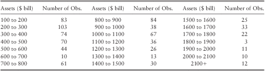
We applied the model described in section 3 to Algorithmics's ‘Algo Opdata’ database. The database contains publicly reported operational losses above USD $1 mill from financial firms around the world. In order to obtain a fairly homogeneous sample of losses we restricted our analysis to data collected from the US banking industry during the 15 year time period from 1-Jan-1994 to 31-Dec-2008 from banks with assets greater than or equal to $100 bill. There are several reasons for excluding banks with assets less than $100 bill from our analysis. Firstly, most of the records for banks with assets less than $100 bill were incomplete as they did not have values for total deposits, total equity, and number of employees. We made an attempt to recover the missing values but were unsuccessful because documents such as annual reports were not publicly available as most of these small banks are not publicly traded. Secondly, since Algo OpData is collected from public sources such as newspapers, court documents, SEC filings etc., we suspected that the reporting bias in small banks could be different from the reporting bias in medium to large scale banks for the following reasons: 1) usually media tend to treat losses in large banks as more newsworthy than losses in small local banks, therefore the probability of data vendor picking up a loss from a media source is greater for a medium to large scale bank than for a small local bank, 2) regulatory disclosure requirements of small banks are different from medium to large scale banksFootnote 8, therefore probability of a loss being publicly disclosed is lower for small banks, 3) disclosures requirements of publicly listed entities are much more greater than for non-listed entities. Given these circumstances we decided to limit our analysis to banks with assets greater than or equal to $100 bill. However, it should be pointed out that limiting the analysis to banks with assets greater than or equal to $100 bill does not discount the significance of the study, since our sample contains 855 data points, with a fair range of banks from $100 bill to $2000 bill in assets as shown in table 2.
The Distribution of the Selected Sample by Total Assets.
In the following section we shall present the preliminary analysis of the chosen sample and a brief description of the potential explanatory variables for model fitting and their descriptive statistics.
4.1 Preliminary Analysis of the Data and the Explanatory Variables
4.1.1 Size
As discussed earlier much of the previous work has suggested an increasing relationship between loss magnitude and the size of the firm. Algo OpData contains several possible quantities that can be taken as a measurement of firm size, namely total assets, total deposits, total equity and the number of employees. We considered each of these variables in the regression analysis to find the one with the highest explanatory power.
4.1.2 Business Lines (BL)
Certain lines of business can be perceived to be more risky than others. Thus, severity of operational losses may depend on the business line. As a preliminary analysis we classified business activity into six business lines and computed the median, 75th, and 99th percentiles of the losses for each business line. The results are given in table 3.
The Summary Statistics by Business Line.
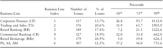
Note 1: Basel II classifies operational losses into eight business lines. Due to the limited amount of data ‘Payment and Settlement’, ‘Agency Services’, and ‘Asset Management’ were grouped together and have been labelled as ‘PS, AS, AM’.
Note 2: All losses are expressed in 2008 dollar terms.
Results show that the highest number of losses have occurred in ‘retail brokerage’ followed by ‘trading and sales’. ‘Corporate finance’ had the highest losses in all three percentiles indicating that this particular business line is relatively riskier than the others. In contrast, retail brokerage had lower severities at all three percentiles.
4.1.3 Event Type (ET)
The type of operational loss is another potential explanatory variable. We categorised losses into five different event types as outlined in table 4. Preliminary analysis showed that more than half of the operational losses were due to ‘clients, products & business practices’ (CPBP). CPBP had large losses at higher percentiles indicating particular event category to be riskier than the others.
The Summary Statistics by Event Type.
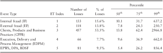
Note 1: Basel II classifies operational losses into seven event types. Due to the limited amount of data the ‘Employment Practices and Workplace Safety’, ‘Damage to Physical Assets’, and ‘Business Disruption and System Failures’ were grouped together and have been labelled as ‘EPWS, DPA, BDSF’.
Note 2: All losses are expressed in 2008 dollar terms.
4.1.4 Equity Ratio
Ideally when modelling operational risk one needs to take into account the internal controls and risk culture of a firm. Unfortunately the Algo OpData does not provide any such information. Therefore, we turned to other publicly available variables which can be used as proxies for risk culture and internal controls.
The first variable we considered was a governance index created by Gompers et al. (Reference Gompers, Ishii and Metrick2003). This index measures shareholder rights in comparison to management power. The index can be considered as a proxy of the quality of governance, assuming that the greater the power held by management, the more likely they are to breach fiduciary duties and adopt ad hoc market practices. However, we found little use of the index since index values were not available for the full sample duration as well as for many small banks in the sample.
Secondly, as an alternative we considered equity ratio as a proxy for the risk taking tendency of the senior management. The Equity ratio of a company is defined as the ratio between shareholders’ equity and total assets. The ratio indicates the proportion of equity used to finance a company's total assets. It is a measure of leverage used as an alternative to the popular debt-to-equity ratio. Since Algo OpData provides information on both assets as well as the shareholder equity, the ratio was readily computable. We hypothesized that a high leverage is an indicator of the overall riskiness of the company and can therefore provide insight into risk culture within the company. If our hypothesis is correct the regression analysis should yield that the variable is positively correlated with the losses.
4.2. Estimating the Weights
The first step in developing the scaling model is to compute weights for the observations by using the techniques discussed in section 3.3. First, we plot a sample mean excess plot of the losses to confirm that the losses belong to a heavy-tailed class of distribution. We find that the mean excess plot has a linear upward trend as expected (see figure 3), which confirms that our data belongs to a distribution that lies in the maximum domain attraction of Fréchet distribution. In other words, distribution of the logarithm of losses should lie in the maximum domain attraction of Gumbel distribution, and therefore, for a high enough threshold one can approximate the excess log-loss distribution to an exponential distribution as described in section 3.3.
Mean Excess Plot of Operational Losses.

It is well known that the GPD approximation works well only if the threshold u is selected properly. If the threshold u is chosen correctly, then for any other threshold v (>u) the estimated parameter values for b should remain equal to the initial estimates. To verify this we estimated the parameters b, τ, and a by maximizing the likelihood equation given in eq. (5) for various thresholds. The estimated parameter values are given in table 5. We find that the parameter values for b and a stabilizes after the $5 mill threshold. Hence, weights were computed using eq. (6) where  $\hat{a}\: = \:0.96$, and
 $\hat{\tau }\: = \:(3.27\: + \:log{\rm{(5)}})$. These weights have been used to estimate all the GAMLSS models presented in the subsequent sections.
Estimation Results b, τ, and a for Various Thresholds.
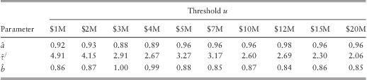
Note: We carried out likelihood ratio tests of the restriction that the reporting probabilities are constant across all losses for each threshold level (i.e. there is no reporting bias in the data). The p-values of the likelihood ratio tests for all the threshold values were less than 0.01, which confirmed the existence of reporting bias.
4.3 Model Selection
4.3.1 Choosing a Base Model
The initial step in model selection is to find a base model having no explanatory variables which closely follows the data. In other words we are seeking an appropriate probability distribution assumption for model fitting. As discussed earlier in section 3.3 operational losses are heavy tailed, hence logarithm of operational losses should belong to a distribution which lies in the maximum domain of attraction of the Gumbel distribution. Distributions within this class exhibit tails with exponential decay. Many thin to medium tailed distributions fall under this class of distributions including the Normal, Lognormal, Exponential, Gamma, Weibull, and Gumbel among others (McNeil et al., Reference McNeil, Frey and Embrechts2005, p. 269). We fitted several of these distributions to the data and computed the AIC values using eq. (2). A list of the distributions we fitted together with their density functions, formulas for mean and variance are given in table 6. The estimated parameter values of the fitted models and their AIC values are given in table 7.
The List of Fitted Distributions.
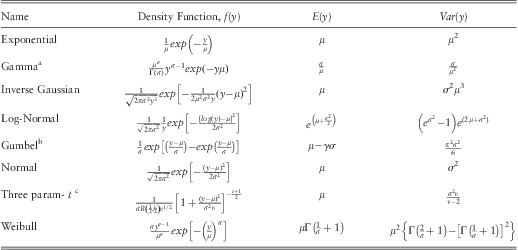
a – Γ(.) is the gamma function.
b – γ is the Euler–Mascheroni constant ≈ 0.5772.
c – B(.) is the beta function.
The Competing Base Models.
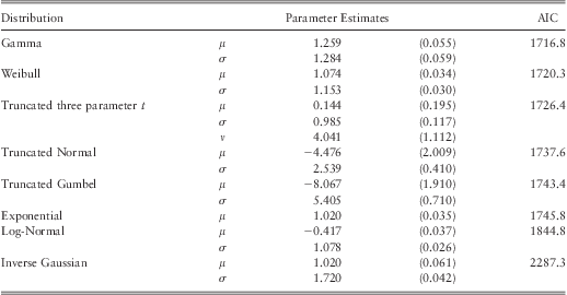
Note: Since only the losses which are above the $1 mill threshold are included in the database the range of the log-losses is y 1∈[0,∞). Hence, truncated versions of Normal, Gumbel, and t-distribution were fitted to the data.
As reported in table 7, the model fitted with the Gamma distribution provided the lowest AIC value. Hence, we chose the Gamma distribution for model fitting.
It is worth pointing out that when the logarithm of a random variable X follows a Gamma distribution, X itself is said to follow a Log-gamma distribution. Log-gamma distribution is a heavy-tailed distribution with a Pareto-type tail behaviour. That is, there exists a slowly varying Footnote 9 function h(.) such that
 $$Pr{\rm{(X}}\: \gt \:x{\rm{)}}\:{\rm{ = }}\:{{x}^{{\rm{ - }}\alpha }} h(x)$$
The parameter α in the above equation is called the tail index of the distribution. The value of α determines the thickness of the tail. The smaller the α, the thicker the tail of the distribution. In other words, extreme observations become even more likely. This particular characteristic makes Pareto-type distributions (which includes Log-gamma) an attractive framework to model operational risk.
The density function of the Log-gamma distribution is given by
 $$f(x)\: = \:\frac{{{{\alpha }^p} }}{{{\rm{\rGamma }}(p)}}{{x}^{{\rm{ - }}\alpha {\rm{ - 1}}}} \,{{[log{\rm{(}}x{\rm{)}}]}^{p{\rm{ - 1}}}} $$
where, Γ(.) is the gamma function, and p and α are the lower and upper shape parameters. The distribution function of the Log-gamma distribution is given as
 $$F(x)\: = \:\frac{{\gamma (p,\,\alpha \log (x))}}{{{\rm{\rGamma }}(p)}}$$
where, γ(.) is the lower incomplete gamma function. The expected value of the Log-gamma random variable is given by
 $$E(x)\: = \:{{\left( {\frac{\alpha }{{\alpha {\rm{ - 1}}}}} \right)}^p} \; \; \; \; \; \; \; \; \; \; \; \; \; \; \; \; {\rm{for}}\ \alpha \: \gt \:1$$
and, the variance by
 $$Var{\rm{(}}x{\rm{) = }}{{\left( {\frac{\alpha }{{\alpha {\rm{ - 2}}}}} \right)}^p} {\rm{ - }}{{\left( {\frac{\alpha }{{\alpha {\rm{ - 1}}}}} \right)}^{{\rm{2}}p}} \; \; \; \; \; \; \; \; {\rm{for }}\ \alpha \: \gt \:2$$
The coordinates (F, L) of the Lorenz curve is given by
 $$\left( {F = \frac{{\gamma (p,\alpha log(x))}}{{\rGamma (p)}},\,L\: = \:\frac{{\gamma (p,(\alpha {\rm{ - 1}})log(x))}}{{\rGamma (p)}}} \right)$$
Note that if X~Log-gamma(α, p) as defined in eq. (8) then a random variable Y = log(X) follows a gamma distribution as defined in table 7 with μ = α and σ = p, where μ is called the rate parameter and σ is called the shape parameter.
The Log-gamma distribution has a finite variance only if α > 2. Moreover, distribution has a finite mean only if α > 1. A distribution with α < 1 is referred to as an extremely heavy-tailed distribution or as an infinite mean model. Such distributions can have important implications for capital calculations as have been pointed out by Nešlehová et al. (Reference Nešlehová, Embrechts and Chavez-Demoulin2006). We shall discuss this issue in detail later in section 4.6.1.
4.3.2 Step-wise Selection of Explanatory Variable
Once the distributional assumption has been established, we carried out a step-wise selection of the explanatory variables discussed in section 4.1 for the parameters μ and σ of the Gamma distribution. The strategy which we used to select the explanatory variables is presented schematically in figure 4.
The Step-Wise Selection Strategy of Explanatory Variables.

The choice of link functions is an important consideration in fitting GAMLSS models. For the Gamma distribution both parameters μ and σ are defined as greater than zero. Therefore, log link function appears to be a suitable candidate for both parameters. However, inverse link function is the canonical link function for Gamma distribution in the GLM frameworkFootnote 10. Hence, we tested models with log link function as well as inverse link function by comparing the AIC values and the normalized quantile residual plots (discussed earlier in subsection 4.4). We found that models fitted using a log link function to μ and σ provided lower AIC values as well as better residual plots. Therefore, log link functions were chosen for both parameters.
As mentioned earlier Algo Opdata provides several possible quantities, namely total assets, total deposits, total equity and number of employees, which could be used to measure the size of a bank. We considered logarithm of each of these variables in the regression analysis and compared the AIC values and the residual plots to find the variables with the highest explanatory power. Both log-assets as well as log-equity provided models with slightly better fit than the models based on log(number of employees) and log-deposits. Given that all these variables are highly correlated it is no surprise that all of them were found to be significant. Since total assets is usually a better measure of the size of a bank and the magnitude of its operations than total equity, and also because previous studies have used total assets for their analysis, we decided to use log-assets in model fitting over log-equity.
The parameter estimates of the final model given by the step-wise selection method is shown in table 8 (denoted as model G). The model has been fitted using retail brokerage as the baseline category for business lines and the event variable ‘EPWS, DPA, BDSF’ as the baseline category for event types.
Estimated Parameter Values for Model G.
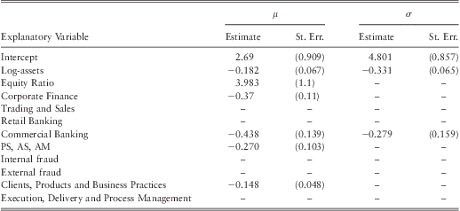
Note: the model is fitted using retail brokerage as the baseline line category for business lines and ‘EPWS, DPA, BDSF’ as the baseline category for event types.
Based on the step-wise selection method outlined earlier we find log-assets, equity ratio, corporate finance, commercial banking, ‘PS, AS, AM’ business lines, and the clients, products and business practices event type are significant explanatory variables to the rate parameter μ. As for the shape parameter σ, log-Assets and commercial banking were found to be significant explanatory variables.
We find that the size of a firm is a significant explanatory variable for both shape as well as the rate parameter of the distribution. In particular, we find a negative correlation between the size of a bank and the rate parameter μ. This implies that the tail of the operational loss distribution becomes heavier with the size variable. This is an important finding since previous studies have mostly focused on the effect of the size of a bank on the mean of the log-loss distribution and had come to the conclusion “…size effect is of little significance in explaining the level of losses” (Dahen & Dionne, Reference Dahen and Dionne2010, p. 1491). A detailed analysis of this important result as well as an interpretation of the estimated parameters will be provided later in subsection 4.6. In the subsequent sections we will present the robustness analysis for the parameter estimates and the model diagnostics.
4.4 Model Diagnostics and Robustness Analysis
4.4.1 Diagnostic Plots
The diagnostics for the fitted model were carried out using a QQ plot of normalized quantile residuals as described in section 3.2. The resulting QQ plot is given in figure 5. The QQ plot indicates that the estimated residuals closely follow a standard Normal distribution. Hence, we concluded that the model provides a reasonable fit to the data.
Normalized Quantile Residual Plot of the Model G.

4.4.2 Robustness of Parameter Estimates
In order to test whether the estimated parameters are robust to model specification and the underlying data we analyzed the following two cases:
1) Model G.1 – refit model G after removing losses above $1 bill in banks with assets greater than $500 bill.
2) Model G.2 to G.11 – sequentially add explanatory variable to a model with only intercept and log-assets as explanatory variables.
The Case 1 test the robustness of the parameter estimates against few extreme losses occurred in large banks. There were 5 losses above $1 billion in banks with assets greater than $500 billion. The refitted model after removing those data points are given in table 9 under the column heading model G.1. We find that the parameter estimates do not vary much from initial estimates. Especially, the coefficient of the size variable remains remarkably stable even after removing the large losses.
The Robustness Analysis.

Since size is an important variable for the scaling model, we analyzed the stability of the coefficient of the size variable with respect to model specification in Case 2, by fitting a series of models with different specifications. We started with model G.2 which only has the log-assets as explanatory variables. Then we sequentially added other explanatory variables to the simple model and tested the stability of the coefficients of the size variable. The results show that the size variable remained relatively stable as well as statistically significant, across all models.
4.5 Validation of the Model by Simulation
As a further validation of the model we simulated losses for the US banking industry, and two individual US banks, and compared the simulated losses against the observed losses. For individual banks we chose two banks with sufficient loss data for statistical estimations. To protect anonymity we shall refer to the two banks as Bank A and Bank B. Bank A had incurred 141 losses and Bank B had incurred 92 losses during the sample period. Both banks were operating continually throughout the sample period. The results of the simulations are presented in the following sections.
4.5.1 Simulating Losses for the US Banking Industry
We simulated 1,000,000 random losses for the US banking industry by using the observed values of the explanatory variables in the fitted model repeatedly. Then we tested the goodness-of-fit by comparing the quantiles of the simulated losses with the observed losses using a QQ plot. Furthermore, we constructed distribution free 95% confidence intervals for the quantiles of the observed losses using the methodology outlined in Arnold et al. (Reference Arnold, Balakrishnan and Nagaraja1992). The resultant QQ plot and the table of some of the selected quantiles with their confidence intervals are given in figure 6 and table 10 respectively.
QQ Plot of Simulated Losses vs. Observed Losses for US Banking Industry. Note: quantiles for the observed losses have been computed using the weights estimated in subsection 4.2.

Summary Statistics of the Simulation for the US Banking Industry.
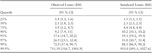
Note 1: percentiles for the observed losses have been computed using the weights estimated in subsection 4.2.
We find that the QQ plot follows a fairly straight line with a unit gradient confirming our model. The model fits particularly well in the lower percentiles of the loss distribution. However, the QQ plot indicates a possible deterioration in the fit towards the tail of the distribution. The reported values in table 10 shows that simulated loss is 9.7% higher than the observed loss at the 95th percentile. At the 99.9th percentile the difference between the simulated and the observed percentiles becomes 34.3%. However, a closer look at the table reveals that the percentiles of the simulated losses lie well within the 95% confidence intervals of the percentiles of the observed losses. Hence, there is not enough evidence to suggest that the model is overestimating the losses. One could observe from table 10 that the confidence intervals of the higher percentiles of the observed losses are fairly wide due to lack of data. This increases the uncertainty of the goodness-of-fit in the tail of the distribution. In such situations one would need to take a conservative approach to assess the goodness-of-fit of the model. Under the given circumstances we believe that the seeming overestimation of the far tail of the distribution by the fitted model will reduce the uncertainty of underestimation of the tail. Thus, this apparent overestimation in the tail can be seen as a strength of the model rather than a weakness. Hence, we conclude that the model provides a reasonable, yet conservative fit, to the data.
4.5.2 Simulating Losses for Two Individual Banks in the US
Our purpose is to build a model that can simulate losses to a bank when there is not enough internal data of their own to assess the tail of the loss distribution accurately. Thus, to verify whether our model can be used for this purpose we re-estimated the parameters of model G by removing the losses incurred in Bank A from the dataset and then simulated 1,000,000 random losses using the new parameter estimates. Similarly, 1,000,000 random losses were simulated for Bank B by re-estimating the parameters of model G by removing the losses incurred in Bank Bfrom the dataset. The QQ plots of the observed losses against the simulated losses are given in figure 7 and figure 8. A summary table of the percentiles and their confidence intervals is given in table 11. The re-estimated parameter values for model G is given in table 12 and table 13.
QQ plot of Simulated Losses vs. Observed Losses for Bank A. Note: quantiles for the observed losses have been computed using the weights estimated in subsection 4.2.

QQ plot of Simulated Losses vs. Observed Losses for Bank B. Note: quantiles for the observed losses have been computed using the weights estimated in subsection 4.2.

Summary Statistics of the Simulation for Bank A and B.
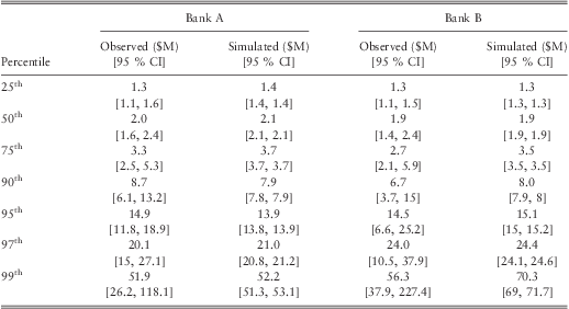
Note: percentiles for the observed losses have been computed using the weights estimated in subsection 4.2.
Re-estimated Parameter Values of Model G after Removing Bank A.
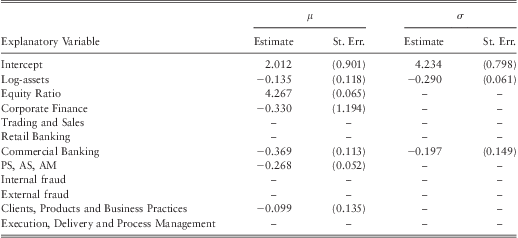
Note: the model is fitted using retail brokerage as the baseline line category for business lines and ‘EPWS, DPA, BDSF’ as the baseline category for event types.
Re-estimated Parameter Values of Model G after Removing Bank B.
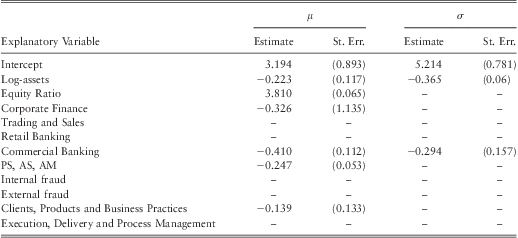
Note: the model is fitted using retail brokerage as the baseline line category for business lines and ‘EPWS, DPA, BDSF’ as the baseline category for event types.
The QQ plots for both banks followed a straight line with a unit gradient confirming our model. table 11 shows that the percentiles of the simulated losses are well within the 95% confidence intervals of the observed percentiles. Hence, the results confirm that the model can be used by individual banks to complement their internal data.
4.6 Interpretation of the Fitted Model
In this section we will analyze how various parameters in the fitted model affect the severity of the loss distribution. In particular, we are interested in how parameters affect the tail index of distribution, 99th percentile loss, and the average operational loss.
4.6.1 The Effect of Size on Operational Loss Severity
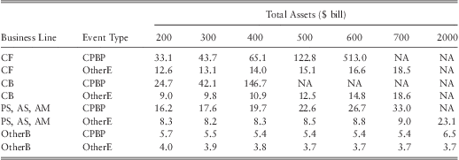
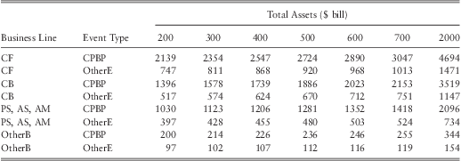
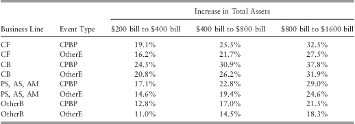
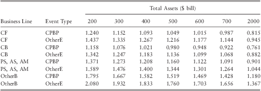
To analyze how the size of a bank may affect its operational loss distribution we consider a series of hypothetical banks with various sizes ranging from $200 bill in assets to $2000 bill in assets. The analysis is carried out by keeping the equity ratio of the hypothetical banks at 6.7%, which is the median equity ratio for US banks in our sample. The computed mean, 99th percentile loss, and the tail index for each bank is given in table 14, table 15, and table 17 respectively. Table 16 provides the percentage change of the 99th percentile of the loss distribution as the size of a bank doubles.
Estimated Average Loss ($ mill).
Note 1 : CF – ‘Corporate finance’, CB – ‘Commercial banking’, PS, AS, AM – grouped business lines of ‘Payment and Settlement’, ‘Agency Services’, and ‘Asset Management’, OtherB – all other business lines, CPBP – ‘Clients products and business practices’, OtherE – all other event types.
Note 2 : All values have been computed by assuming an equity ratio of 6.7%.
Note 3 : NA refers to situations with infinite means.
Estimated Loss at the 99th Percentile ($ mill).
Note 1 : CF – ‘Corporate finance’, CB – ‘Commercial banking’, PS, AS, AM – grouped business lines of ‘Payment and Settlement’, ‘Agency Services’, and ‘Asset Management’, OtherB – all other business lines, CPBP – ‘Clients products and business practices’, OtherE – all other event types.
Note 2 : All values have been computed by assuming an equity ratio of 6.7%.
The increase in the 99th percentile loss when the size of the bank doubles.
Note 1 : CF – ‘Corporate finance’, CB – ‘Commercial banking’, PS, AS, AM – grouped business lines of ‘Payment and Settlement’, ‘Agency Services’, and ‘Asset Management’, OtherB – all other business lines, CPBP – ‘Clients products and business practices’, OtherE – all other event types.
Note 2 : All values have been computed by assuming an equity ratio of 6.7%.
The results in table 14 show that mean loss severity for most BL/ET categories increases with the size of the bank. The baseline combination ‘OtherB-OtherE’ is the main exceptionFootnote 11. It is somewhat puzzling why we may observe a decreasing relationship between severity of loss and the size of the bank in this particular BL/ET category. However, a previous study by Cope & Labbi (Reference Cope and Labbi2008) had also reported similar findings. Given that 57% of the number of losses in this category were due to fraud (which accounted for 69.6% of the total loss in this category), our results are consistent with the findings reported by Cope & Labbi (Reference Cope and Labbi2008) where they have reported a decreasing relationship between fraud related loss severities and the size of a bank. One possible explanation for this phenomenon is that as banks become larger they will have access to more sophisticated IT systems, internal controls, and audit methods which can reduce fraud, leading to a decreasing relationship between average loss severity between fraud and the size of a bank.
However, although the mean loss may decrease for some BL/ET categories, we find loss at the 99th percentile increases for all BL/ET combinations as the size of a bank increases (see table 15). The results in table 16 show that for certain BL/ET combinations 99th percentile loss can increase by up to 25% to 35% when the size of a bank doubles. This is an important result as it proves (contrary to previous studies) that the size of a bank is in fact an important determinant of the severity of operational losses. In particular, the fitted model suggests that large banks are exposed to more tail risk than small banks.
Another way of quantifying the size effect is to compute the tail index implied by the fitted model for banks of various sizes. The results presented in table 17 show that the tail index decreases for all BL/ET combinations as the firm size increases. For almost all BL/ET combinations the tail index is less than 2. That is, the variance of the loss distribution is infinite (which is usually considered as a characteristic of a heavy-tailed distribution). In addition, we find that for very large banks the tail index becomes less than 1 for certain BL/ET categories. That is, the losses follow an extremely heavy-tailed distribution and hence the mean is infinite. Losses which follow an extremely heavy-tailed distribution can have serious implications on capital calculations as well as risk management for banks. Nešlehová et al. (Reference Nešlehová, Embrechts and Chavez-Demoulin2006) provide a detailed discussion on these issues and the challenges of modelling operational risk with extremely heavy tailed behaviour. The following discussion draws on their paper.
Estimated Tail Indices.
Note 1 : CF – ‘Corporate finance’, CB – ‘Commercial banking’, PS, AS, AM – grouped business lines of ‘Payment and Settlement’, ‘Agency Services’, and ‘Asset Management’, OtherB – all other business lines, CPBP – ‘Clients products and business practices’, OtherE – all other event types.
Note 2 : All values have been computed by assuming an equity ratio of 6.7%.
Nešlehová et al. (Reference Nešlehová, Embrechts and Chavez-Demoulin2006) point out that for loss distributions which follow a Pareto-type tail behaviour (i.e., as in eq. (7)), the Value-at-Risk (VaR) grows exponentially as α decrease. Therefore, when α tends to zero the capital charge computed by VaR could become ridiculously high. The fitted model suggests that use of VaRγ can become problematic for large banks since losses in some BL/ET combinations may be extremely heavy-tailed. A one possible solution for this problem is to implement a minimum probability threshold as suggested by Evans (Reference Evans2001). The author states that “a reasonable value judgment may be that events which have less than a 1 in 1,000,000 chance of happening should simply be ignored”. However, for the fitted model we find a higher probability limit of 1 in 10,000 would be required to obtain capital estimates consistent with the industry standards for very large banks. We shall revisit this issue in detail later in section 5 when we compute capital estimates.
Here, one might be tempted to argue that infinite mean models should not be used to model operational losses since the total capital existing is finite. Nešlehová et al. (Reference Nešlehová, Embrechts and Chavez-Demoulin2006) point out that one shouldn't shy away from infinite mean models as financial literature is full of power law models which have some infinite moments, and yet they are used frequently. However, authors do warn that a transition from infinite second moment to infinite first moment requires careful handling.
The second issue of infinite mean models is related to diversification of risk. Often in practice the operational risk capital charge is determined by computing VaRγ for each business line and adding them up as
 $${\rm{Va}}{{{\rm{R}}}_{{\rm{99}}{\rm{.9\% }}}}(L)\: = \:\mathop{\sum}\limits_{k = 1}^K {{\rm{Va}}{{{\rm{R}}}_{{\rm{99}}{\rm{.9\% }}}}({{L}_k})} $$
where, L is the total loss random variable of the bank, and Lk are the total loss random variables for business lines k = 1, …, K. Then, if the bank can demonstrate a reduction in risk due to correlation, a capital reduction would be allowed from the latter. As per our findings this particular method of capital calculation creates several problems. Firstly, we find operational losses are heavy-tailed (i.e. α < 2) for most BL/ET combinations as reported in table 17. In this context a diversification reduction based on correlation makes no sense since correlation coefficients are not defined when α < 2. Secondly, for large banks we find α can become less than 1 for certain BL/ET combinations. Under these conditions (i.e. α < 1) VaRγ is no longer a coherent risk measure Footnote 12 since the subadditivity property
 $${\rm{Va}}{{{\rm{R}}}_\gamma }(L)\: = \:{\rm{Va}}{{{\rm{R}}}_\gamma }\left( {\mathop{\sum}\limits_{k = 1}^K {{{L}_k}} } \right)\:\leq \:\mathop{\sum}\limits_{k = 1}^K {{\rm{Va}}{{{\rm{R}}}_\gamma }({{L}_k})} $$
will no longer hold. Rootzén & Klüppelberg (Reference Rootzén and Klüppelberg1999) and Nešlehová et al. (Reference Nešlehová, Embrechts and Chavez-Demoulin2006) provide several examples of situations in which subadditivity property is violated by VaR under extremely heavy-tailed distributions. In particular, Nešlehová et al. (Reference Nešlehová, Embrechts and Chavez-Demoulin2006) show that for independent business lines having Pareto-type risks (i.e. a tail behaviour of the form eq. (7)) with 0 < α < 1
 $${\rm{Va}}{{{\rm{R}}}_\gamma }\left( {\mathop{\sum}\limits_{k\: = \:1}^K {{{L}_k}} } \right)\: \gt \:\mathop{\sum}\limits_{k\: = \:1}^K {{\rm{Va}}{{{\rm{R}}}_\gamma }({{L}_k})} $$
for sufficiently large γ. In other words, when losses are distributed as in an infinite mean model diversification no longer exists in the traditional sense under the VaRγ measure. The authors state that “…in the presence of extremely heavy-tailed loss distributions, standard economic thinking may have to be reconsidered” and we “…have to accept that a VAR-based risk-capital calculation for operational risk is not yet fully understood”. The tail index estimates given in table 17 indicates that the banks with assets greater than $500 bill should take extra concern about these issues.
Usually subadditivity is considered an important property for a risk measure as it promotes diversification. However, as has been pointed out by Rootzén & Klüppelberg (Reference Rootzén and Klüppelberg1999) subadditivity does not necessarily need to hold for catastrophic risk. By using a simple example authors show that combining two catastrophic risks will increase the probability of ruin rather than decrease it. The authors state that “big is not always beautiful” and “catastrophic financial risks don't become smaller if collected in one big company”. Hence, non-subadditivity of VaRγ when α < 1 should not be considered as a limitation of the risk measure. However, risk managers should keep in mind that when operational losses follow extremely heavy-tailed distributions, simply adding up the capital estimates for each business lines would not provide a conservative estimate as it would provide in most other types of risk. This issue would be particularly important to banks with assets greater than $500 bill in which tail index of operational losses can become less than 1 as seen from table 17.
The final point we would like to raise is the one-loss-causes-ruin problem of operational risk. The one-loss-causes-ruin problem refers to the phenomena that a significant portion of total losses are caused by few individual losses. This phenomena can be illustrated by the use of a Lorenz curve. The concept of a Lorenz curve is used in economics to analyze inequality of income distribution (and wealth) in a population. A related concept to the Lorenz curve is Pareto's famous 80:20 law which states “80% of the all effects results from 20% of the causes”. The 80:20 law has been observed in many economic and natural processes and is referred to as law of the vital few. (see Ultsch, Reference Ultsch2002, to find many situations in which Pareto's 80:20-law is reported). The 80:20 law applies when outcomes of interest follow an exact Pareto distribution with α ≈ 1.16096. If operational losses follow the Pareto law, then 80% of the total loss would be caused by 20% of the individual losses. Hence, the threat to a bank's solvency would be mainly driven by those 20% large individual losses. To see whether such a pattern exists in operational losses, we computed the implied Lorenz curves by the fitted model for each BL/ET combination for two hypothetical banks with $300 bill assets and $600 bill assets respectively, using eq. (12). The plots of the resulting curves are given in figure 9 and figure 10. By comparing the two plots one could observe that the percentage of total loss caused by few extreme losses is high at the larger bank. To illustrate this further, we have reported values of the Lorenz curve for selected percentages in table 18 and table 19. The value given in the first row of the third column of table 18 indicates that for a bank with $300 bill assets 80% of the total loss due to CF-CLBT is caused by 7% of the individual CF-CLBT losses. In contrast, the third row of the first column in table 19 indicates that for a bank with $600 bill assets, 80% of the total loss due to CF-CLBT category is caused by only 0.5% of the individual CF-CLBT losses. Similar results hold for CB-CLBT combination as well. Moreover, the first row of the fifth column in table 19 indicates that for a bank with $600 bill assets, 99% of the total loss due to CF-CLBT category is caused by only 1.83% of the individual CF-CLBT losses. This is an important result which should serve as a warning to large banks about the heavy-tailedness of the risk in these particular BL/ETs. Our results suggest that the one-loss-causes-ruin problem is relevant for small as well as for large banks, but it is much more severe for large banks. The complexity of banking activity at large banks can probably be the reason for this. Furthermore, results suggest that the problem seems to be rooted in the CPBP event category. Hence, more care should be given when modelling this type of risk.
The Lorenz curves of the loss distributions at a bank with 300 bill assets. Note: an equity ratio 6.7% has been assumed to compute the Lorenz curve.

The Lorenz curves of the loss distributions at a bank with 600 bill assets. Note: an equity ratio 6.7% has been assumed to compute the Lorenz curve.

Cumulative % of individual losses as the % of total losses.
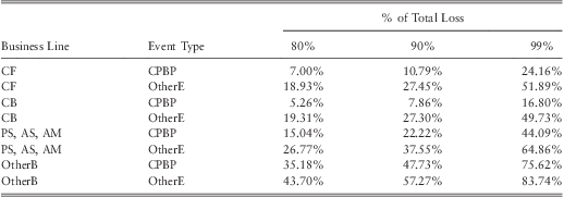
Note: an equity ratio of 6.7% has been assumed to compute the above values.
Cumulative % of individual losses as the % of total losses.
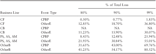
Note: an equity ratio of 6.7% has been assumed to compute the above values.
4.6.2 The Effect of Equity Ratio on Operational Loss Severity
In section 4.1.4 we hypothesized that the equity ratio can be used as a proxy to the risk culture within a bank. At this point, we shall test the validity of that hypothesis by analyzing how equity ratio affects the operational loss severity as suggested by the fitted model.
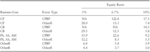
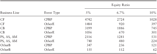
Table 20 and table 21 provides the fitted mean and the 99.9th percentile loss for banks with $500 bill assets and an equity ratio of 5%, 6.7%, and 10%. Both tables indicate that the severity of operational losses are high for the bank with a low equity ratio. In particular, we find severity at the 99.9th percentilecould increase by around 40% to 70% (for certain BL/ET up to 75%, e.g., CF-CPBP) when the equity ratio drops from the median ratio of 6.7% to 5%. Similarly, when the equity ratio increases from 6.7% to 10% losses at the 99.9th percentile drop by around 40% to 60%.
Estimated Average Loss ($ mill).
Estimated Loss at the 99th Percentile ($ mill).
The above results suggest that our initial hypothesis that the equity ratio may serve as a proxy for the risk culture of a bank is valid. However, a word of caution is required here as the hypothesis may not hold universally for all banks, since the equity ratio is not a direct measure of the risk culture of a firm. Usually a low equity ratio does not necessarily mean a firm is too risky. It could well mean that the management is efficient in investing the equity capital. Similarly a too high equity ratio could be a sign of management wasting resources.
We conclude this section by providing a brief summary of the main inferences we gathered from the fitted model and the issues we have raised so far. As discussed earlier, the estimated parameters of the model suggest that the size of a bank is an important indicator of its operational loss severities. In particular, model indicate there is a considerable variation in the tail index of the loss distribution across banks of different sizes. This is an important result which may have a significant impact in terms of capital calculation as well as risk management. As we have pointed out, the tail index for certain BL/ET combinations can become less than 1 for very large banks. Although capital can be computed using the VaR method under these conditions, the computed capital can be too high. A possible solution for this is to implement a minimum probability threshold. The second issue one needs to be careful of is that VaR is no longer subadditive when α < 1. Hence, one should not compute the total required capital by adding up the VaR estimates of each business line. We find these particular issues are more relevant to large banks than to small banks as the tail index for small banks tends to be in the region of α > 2. Furthermore, the estimated parameters suggest that both small as well as large banks are subject to the one-loss-causes-ruin problem, but the exposure is severe for large banks. Particularly, this raises the importance of scenario analysis as well as having a sound crisis management system in place to handle catastrophic events.
5 Capital Calculation
This section provides a demonstration of the severity model at work by computing capital estimates for several hypothetical banks as well as for two real banks by making simple assumptions about the frequency distribution. The results show that the capital estimates are reasonable and consistent with the industry standards.
5.1 Capital Estimates for Hypothetical Banks
In order to compute capital estimates one would need a frequency distribution for operational losses. Here, we make the simple assumption that the loss frequency in each BL/ET category is distributed as a Poisson random variables with a density function
 $$Pr{\rm{(}}{{N}_j}\: = \:{{n}_j}{\rm{)}}\,\:{\rm{ = }}\,\:\frac{{\lambda _{j}^{{{{n}_j}}} {{e}^{{\rm{ - }}{{\lambda }_j}}} }}{{{{n}_j}!}}$$
where nj is the number of losses above $ 1million and λj is the Poisson parameter of the j th BL/ET category for j = 1, …, 30. The maximum likelihood of parameter of λj is the sample mean of the loss frequency in BL/ET category j. This makes the Poisson assumption particularly attractive in the current context, since estimation becomes very easy as data on average frequency of losses is publicly available. However, a limitation of the Poisson distribution is that its variance is equal to its mean. Hence, other distributions such as Negative Binomial would be more suitable if one needs to allow for more variation in the frequency model. However, it is a well known fact that for compound distributions of the form  $S = \sum _{{i\: = \:1}}^{N} {{X}_i}$, where, Xi are subexponential severities with distribution function F and the frequency distribution given by Pr(N = n) = p(n), if there exist a constant ω > 0 such that
 $$\mathop{\sum}\limits_{n\: = \:0}^ \propto {{{{(1\: + \:\omega )}}^n} p(n)\: \lt \:\infty } $$
then the aggregate loss distribution G is subexponential with tail behaviour given by
 $$\bar{G}(s)\: = \:E(N)\,\:\bar{F}(s)$$
In other words, for heavy tailed losses, the tail of the compound distribution is simply the expected number losses times the tail of the severity given that frequency distribution satisfies the condition given in eq. (13) Footnote 13. This means capital requirement for heavy-tailed risk such as operational risk is mainly driven by the expected number of losses, and therefore over-dispersion is not a major concern. For this reason as well as for its simplicity the Poisson distribution remains a common distributional assumption for modelling operational loss frequencies (see for example De Fontnouvelle et al., Reference De Fontnouvelle, Dejesus-Rueff, Jordan and Rosengren2006; De Fontnouvelle et al., Reference De Fontnouvelle, Rosengren and Jordan2007; Medova & Berg-Yuen, Reference Medova and Berg-Yuen2009). Thus, we believe the assumption is reasonable for the purpose of demonstrating the severity model.
In practice, banks are required to model the dependence structure when computing capital estimates. It is typical to assume dependence between frequencies while severities are assumed independent. Due to data limitations we are unable to model the dependence between frequencies of each business line-event type combination. Hence, we assume that the frequency distribution of each BL/ET combination is independent. Although this is a strong assumption, Basel (2009) reports that modelling of dependence at a typical bank results in a modest 8.3% increase in the economic capital relative to the assumption of full independence. Therefore, we argue that the independence assumption will not affect the results significantly.
Given our assumption that the frequency distribution of each BL/ET combination is independent, the distribution of total frequency  $N\: = \:\sum _{{j\: = \:1}}^{{30}} {{n}_j}$ has a Poisson distribution with a parameter
 ${\rm{\rLambda }}\: = \:\sum _{{j\: = \:1}}^{{30}} {{\lambda }_j}$. This is a direct consequence of the property that the sum of independent Poisson random variables also has a Poisson distribution. To calibrate the parameter Λ, we used the results published by the Basel Committee on the 2008 Loss Data Collection Exercise (LDCE) (Basel, 2009). Table ILD9 in that paper reports that a typical bank experienced 0.013 losses per year of €1 mill (US $1.58 mill) or more for each €1 bill (US $1.58 bill) in assets. Hence, it is reasonable to approximate
 $\widehat{\rLambda }\: = \:0.00823$ for each US $1 bill in assets. Then, the parameter values of λj can be computed by
 $${{{\rm{\widehat{\lambda }}}}_j}\: = \:\frac{{\sum w_{j}^{/} }}{n}{\rm{\widehat{\rLambda }}}$$
where,  $\sum w_{j}^{/} $ is the sum of normalized weights given by eq. (6) for the j th BL/ET combination and n is the total number of observations in the data sample. Table 22 provides the estimated values of
 ${{{\rm{\widehat{\lambda }}}}_j}$ for a bank with $100 bill assets.
Estimates of  ${\rm{\hat{\lambda }}}j$ for a bank with $100 bill assets.
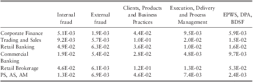
We computed the operational risk capital requirement for 21 hypothetical banks of various sizes and equity ratios by using the above frequency model and the severity model G of section 4.3. The capital estimates for the 21 banks are given in table 23. The results presented in the second row of table 23 have been computed using the median equity ratio of 6.7%. Hence, the results given in the second row can be considered as the required operational risk capital to cover losses above $1 mill for a “typical” bank of a given size, as suggested by the fitted model. The 2008 LDCE of the Basel Committee reports that the median ratio between the reported regulatory operational risk capital and the total assets for a “typical” North American bank is 0.38% (Basel, 2009). The last row of table 23 presents benchmark capital estimates based on this ratio. One could use these benchmark estimates to compare the results presented in the second row of the table to test the reasonability of the capital estimates provided by the fitted model. However, it should be noted that the benchmark capital estimate is the required capital to cover the total operational risk of a bank, as implied by the LDCE report, whereas the capital estimates of the first three rows in the table provide the required amount of capital to cover losses exceeding $1 mill.
Capital Estimates (in $ mill) for Hypothetical Banks.
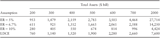
Note: The first three rows of the table gives the capital estimates provided by the severity model G and the frequency model presented in section 5 using 10mill years of simulations. The estimated values are the amount of capital needed to cover losses exceeding $1mill. Additional capital may be required to cover losses less than $1mill if the bank has not priced them into their fees and charges. The last row provides the median (total) operational risk capital held by a typical bank in North America as implied by the ratios given in table C1 of Basel's LDCE report (2009).
One can observe from table 24 that the capital estimates given by the fitted model for a “typical” bank with assets ranging from $200 bill to $700 bill is around 3% to 20% less than the industry benchmark. This is expected, given that our estimates are the amount of capital needed to cover losses above $1 mill, whereas the benchmark capital estimate is the amount of capital needed to cover the total operational risk. Furthermore, our simplified assumption that the frequencies of each BL/ET are independent, would reduce our capital estimates by around 8.3% as explained earlier. Given these facts, we conclude that the capital estimates provided by our model for the first six banks (i.e. banks with assets of $200 bill to $700 bill) are reasonable as well as consistent with industry standards. However, the estimated capital for a bank with $2000 bill assets by our model is $ 14.25 bill, which is 1.87 times larger than the benchmark estimate. Although the estimate is significantly higher than the benchmark, it is in no means an unrealistic estimate. The ratios given in table C1 of LDCE report (Basel, 2009) suggest that the 75th percentile of the regulatory capital reported by a bank with $2000 bill assets was in the range of $11.6 bill to $16 bill.
Capital Estimates (in $ mill) for Hypothetical Banks after implementing a 1-in-10,000 year probability limit.
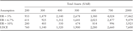
Note: The first three rows of the table gives the capital estimates provided by the severity model G and the frequency model presented in section 5 using 10mill years of simulations. The estimated values are the amount of capital needed to cover losses exceeding $1mill. Additional capital may be required to cover losses less than $1mill if the bank has not priced them into their fees and charges. The last row provides the median (total) operational risk capital held by a typical bank in North America as implied by the ratios given in table C1 of Basel's LDCE report (2009).
The reason behind our capital estimates for large banks being significantly high are the infinite mean models we obtained earlier for certain BL/ET categories in those banks. As discussed in subsection 4.6.1 a solution for high capital estimates yield by infinite mean models is to use a probability limit. We tested several probability limits and found a limit of 1-in-10,000 years would yield capital estimates which are consistent with the industry benchmark. The capital estimates after implementing the probability limit is given in table 24. Note that the probability limit is only implemented when simulating losses from infinite mean models. Hence, capital estimates do not change for small banks in which severity models for all BL/ET categories had tail indices greater than one.
5.2 Backtesting for Two US Banks
In practice regulators require banks to backtest their operational risk models to test whether the estimated capital from the model is sufficient to cover past loss experience. To see how our model performs against such a test we carried out backtesting for Banks A and B of subsection 4.5. The backtesting was carried out using the frequency model described in subsection 5.1 and the severity model given in table 12 and table 13.
The plots of the logarithm of estimated capital and the total log-losses for bank A and B are given in figure 11 and figure 12. The Y-axis of the plots has not been labelled to protect anonymity of the banks. Both plots indicate that the estimated capital is sufficient to cover losses above $1 mill. Furthermore, we find that under the null hypothesis of model being ‘correct’, non-rejection region for number of exceptions (X) based on the Kupiec's POF test (Kupiec, Reference Kupiec1995) is 0 ≤ X ≤ 2 for the 95% confidence level and 0 ≤ X ≤ 1 for the 99% confidence level. The results of the backtest are well within the non-rejection regions for the both confidence levels. Hence, we conclude that the backtesting results further validate our severity model.
Backtesting Results for Bank A.

Backtesting Results for Bank B.

6 Conclusion and Discussion
One of the major challenges of quantifying operational risk for banks is addressing the issue of lack of data. Most of the large operational losses are infrequent and therefore it is impossible to model these losses by solely relying on bank level data. As a solution to this Basel II requires banks to use industry wide external data to complement their internal data. However, combining internal data with external data raises further issues. In this paper we have demonstrated how external data collected from various banks of different sizes and different unknown loss reporting thresholds can be combined together to quantify the operational risk of a bank of a given size.
Two of the main challenges in combining data from different banks is the presence of scale bias and reporting bias. We used a method based on extreme value theory developed by De Fontnouvelle et al. (Reference De Fontnouvelle, Dejesus-Rueff, Jordan and Rosengren2006) to compute inverse probability weights to correct for reporting bias. Then using those weights a regression analysis was carried out to determine the relationship between the loss severity and the size of banks, in order to correct for the scale bias. Most of the previous work had studied only the relationship between the mean of the log-losses and the size of a bank. We argue that a model which only accounts for the scaling in the mean of the log-loss distribution would not be able to capture the tail behaviour of operational losses properly, which is the main interest for capital calculation. A good scaling model should be able to account for the variation in location, scale and shape of the distribution across different business lines and event types. Hence, all the parameters of the distribution should be tested for scaling properties. To achieve this we employed the recently introduced GAMLSS framework to carry out the regression analysis. The model selection process revealed that the operational losses are best explained by a log-gamma distribution with both distributional parameters being related to the size of the bank.
We validated the fitted model by simulating losses for the US banking industry, and two individual banks in the US. Tests demonstrated that the simulated losses follow the observed losses reasonably well. Furthermore, a capital calculation exercise for several hypothetical banks by using simplified assumptions about the frequency distribution revealed that the capital estimates provided by the model is consistent with the industry standards. In addition, backtesting of the model using two US banks also confirmed the validity of the model.
The results of this study suggest that the size of a bank is an important indicator of its operational loss severities than previous research has suggested. In particular, the model indicates that there is a considerable variation in the tail index of the loss distribution across banks of different sizes. We find that for certain BL/ET combinations, 99th percentile loss can increase by up to 25% to 35% when the size of a bank doubles.
An important observation we make is that the tail index for certain BL/ET categories can become less than 1 for very large banks. That is, the loss distribution of certain BL/ET categories is extremely heavy-tailed for very large banks. This can have significant implications for capital calculation as well as for risk management as discussed in the text. In particular, the results show that the loss distribution of CPBP events is extremely heavy-tailed and a significant proportion of the total loss due to CPBP events is caused by a few individual catastrophic losses. This phenomenon is referred to as the one-loss-causes-ruin problem and creates further challenges to estimating the tail of the loss distribution. Although the use of external data as outlined in this paper can improve the estimation of the tail of the loss distribution, given that catastrophes are high degree unique events, the importance of using scenario analysis cannot be stressed enough in this particular context. However, it should be noted also that scenario analysis also has its limitations since dreaming up worst-case scenarios are often very difficult for a number of reasons. Therefore, we stress the importance of having a system to monitor near-miss losses for early detection of possible crises and having a well established crisis management system in addition to the risk management system to assist a bank to steer through a catastrophic event.
The scaling model developed in this study is of particular importance to banks, as it can be used to complement their internal data and improve the estimates of the tail of the distribution. For example, it is possible to estimate the tail index of the operational loss distribution of a particular bank as  $\hat{\alpha }\: = \:{\rm{\omega }}{{\hat{\alpha }}_{Int}}\: + \:(1{\rm{ - }}\omega ){{\hat{\alpha }}_{Ind}}$, where
 ${{\hat{\alpha }}_{Int}}$ is the estimate of the tail index given by the bank's internal data,
 ${{\hat{\alpha }}_{Ind}}$ is the estimate of the tail index given by the proposed model using industry data, and ω is a credibility weight decided by the experts. The bank could assign a higher weight to the internal estimate
 ${{\mathop{\alpha }\limits^{\frown}}_{Int}}$ if it has satisfactory amount of high-quality data, however when the quality of internal data is poor or not relevant due to a recent change in the operational environment such as a merger or an acquisition, the bank will need to assign a higher weight to the external estimate
 ${{\hat{\alpha }}_{Ind}}$. In practice, ad hoc procedures are often used to decide the credibility weights. However, it is also possible to use a full credibility theory approach to combine the internal and external estimates as proposed by Bühlmann et al. (Reference Bühlmann, Shevchenko and Wüthrich2007) and Lambrigger et al. (Reference Lambrigger, Shevchenko and Wüthrich2007). Another use of the proposed model is that it can serve as a good starting point for building internal models and as a reference for the banks as well as the regulators when examining the appropriate capital levels. We consider the model is an improvement over the existing models found in the literature for two main reasons: 1) it takes into account the scaling properties of all the parameters in the loss distribution rather than just the location parameter, and 2) the scaling properties of the tail index are explicitly modelled, which is more significant to the capital calculation rather than the mean of log-losses. However, a major limitation of our model is that simulated losses are not sensitive to the internal controls of a bank. Therefore it would be interesting to extend the model to include other explanatory variables that reflect the quality of risk management and governance of individual banks. For example, variables such as the annual risk management budget and the cost of employee training might be able to serve as proxies for the quality of risk management and staff competence. The number of past fiduciary breaches and regulatory fines may serve as proxies for the quality of corporate governance. We believe an extension of our model which takes into account the internal controls would provide better capital estimates which reflect the individual circumstances of the banks. However, in order to facilitate such study the industry will need to be generous enough to share some of their confidential data with academia.



