It is an axiom of Brazilian history that railroads favored an extreme specialization in agricultural exports, dependence on foreign inputs, and an excessive need for overseas financial capital, which together subverted the development of domestic-use activities, drained profits, and undermined the benefits of cheaper transport.1
See, for example, Stein and Stein, Colonial Heritage, pp. 147–50; Frank, Capitalism, pp. 168–69; Burns, History, 160–71; Evans, “Continuities” pp. 33–35; Halperin Donghi, Contemporary History, pp. 122–23; Bulmer-Thomas, Economic History, p. 106; Melo, “Investimentos Ferroviários,” passim; and Mello, Capitalismo Tardio, pp. 84–92.
Brazil indeed negotiated most of the nineteenth century with little or no increase in per capita output.
2 Estimates of Brazilian economic growth necessarily rely on indirect indicators; Contado and Haddad, “Produto Real”; and Leff, Underdevelopment, pp. 29–43.
Long-cherished
dependentista accounts assign much of the blame for underdevelopment to the country's export orientation and its reliance on foreign finance, both of which the railroad presumably exacerbated. To date such claims remain largely untested.
3 Leff conjectured that railroads impelled growth, but did not use evidence from the transport sector; Underdevelopment, pp. 146–49. Saes first identified the striking role that São Paulo's railroads played in promoting domestic-use activities; Saes, Ferrovias, pp. 99–120.
This article assesses the railroad's direct and indirect effects in Brazil, where high transport costs posed a major obstacle to economic growth in the nineteenth century.
Brazil stood apart from the conventional patterns of railroad development. The direct impact of the railroad, surprisingly limited in advanced industrial nations, proved quite large in some relatively backward economies. Small social savings in high-income countries with sizeable transport sectors resulted from low-cost substitutes for the railroad, typically in the form of affordable inland navigation.4
Fogel, Railroads, pp. 17–110; Fishlow, American Railroads, pp. 18–62; Vamplew, “Railways,” pp. 47–53; Hawke, Railways, pp. 187–96; Caron, “France,” pp. 42–46; Fremdling, “Germany,” pp. 137–40; and Laffut, “Belgium,” pp. 216–21.
Where navigable waterways were absent from productive regions, or topography did not permit affordable wagon roads, the railroad created substantial unit-cost savings on moving freight and people. Laggard economies with sufficiently high levels of transport services thus received comparatively larger direct benefits from the new technology.
5 Coatsworth, Growth, pp. 77–119; Gómez Mendoza, Ferrocarriles, pp. 63–120; Herranz-Loncán, “Railroad Impact,” pp. 3–13; Summerhill, “Argentine Railroads”; and Crafts, “Social Savings,” p. 2. Lower social savings elsewhere stem in part from inland waterways or low shares of transport in total output; White, “Concept,” pp. 82–101; Metzer, Economic Aspects, pp. 26–52; McGreevey, Economic History; Ramírez, “Ferrocarriles,” pp. 83–90; Huenemann, Dragon, pp. 220–29; and Mata and Tavares, “Value,” pp. 21–24.
The railroad's backward linkages were not strong anywhere in the aggregate, but advanced economies were able to provision the bulk of their railroad inputs from domestic sources.
6 Railroads did not account for the bulk of industrial output of any sector, save for Bessemer steel in the United States; O'Brien, “Transport,” p. 355. Where resources existed railroads could spark the development of new industry, even though most output eventually went to other uses; Fremdling, “Railroads” and “Germany,” pp. 123–31.
Laggards could reap the benefits of technological advance by importing their railroad inputs, but also bore foreign exchange costs, and exported income and employment effects that, in the cases of more advanced economies, were captured domestically. Forward linkages varied considerably, but in cases taken as representative of backward economies the railroad magnified their comparative advantage as primary producers and commodity-exporting nations.
7 Though the export stimulus is viewed as strong, the extent of the effect is in dispute in the Mexican case; Summerhill, “Argentine Railroads”; Metzer, “Railroad Development,” pp. 541–49; Coatsworth, Growth, pp. 122–33; and Kuntz Ficker, Empresa Extranjera, pp. 211–348.
Despite the large system of navigable waterways concentrated in Brazil's north and west, most production and commerce was located elsewhere. The introduction of the railroad in regions south of the Amazon during the second half of the nineteenth century economized substantially on the costs of movement. Large freight social savings were the chief result and contrasted with smaller gains from railroad passenger services. Estimates of the social rate of return reveal that Brazil likely underinvested in railroads in the aggregate, while simultaneously overinvesting in particular lines. Weak backward linkages diluted the full development potential of the railroad, but, in contrast to dependentista characterizations, the foreign-exchange costs of overseas inputs were low. Strong forward linkages were evident in the inflows of immigrants and capital formation in manufacturing and export agriculture. Forward linkages nonetheless heavily favored the domestic market. The railroad led Brazil's transition to growth, positioning the country to become one of the most rapidly expanding economies in the western world for much of the twentieth century.8
For the first eight decades of the twentieth century Brazil out-performed the major economies of the developed and developing western world, with the exceptions of Finland and Norway; Maddison, “Comparison,” pp. 27–41, and World Economy, p. 15.
Post-1850 transport policies responded to the demands for cheap transport by the planter class, creating the first railroad subsidies.9
Benévolo, História Ferroviária, pp. 104–654, passim. Detail on concessions and guarantees found in Paiva, Legislação Ferroviária; Sá, Código da Viação Ferrea; and Cunha, Estudo Descriptivo.
Construction began in 1852, and in the ensuing decades domestic capitalists, foreigners, and the government itself all invested in railroad projects. In the 1870s Brazil assiduously courted new railroad investment. The 1873 railroad law attracted new capital and strove to redress the early stark concentration of railroads in a few provinces of the center-south and northeast.
10 Legislation from Pessôa, Estudo Descriptivo; Coruja, Repertório; Sá, Código; and Paiva, Legislação Ferrovidária.
By 1890 central and state governments had granted some 255 concessions for trunk lines and extensions, most of which never left paper.
11 Sá, Brazilian Railways, tables following p. 40.
Bringing concessions to fruition required dividend guarantees to investors. Guarantees underwrote at least part of the operation of nearly all of the major rail lines, many of which needed subsidies every year.
12 Summerhill, “Market Intervention,” 544–49; promotion efforts in São Paulo are particularly well documented; Lewis, Public Policy, pp. 4–50.
From only a few hundred kilometers of track in the 1860s the system expanded to more than 24,000 kilometers in 1913.13
The fall in the prices of key inputs, such as steel rails, aided in accelerating investment; Brasil, Instituto Brasileiro de Geografia e Estatística (hereafter IBGE), Repertório Estatístico, p. 46; Mitchell, British Historical Statistics, p. 763; U.S. Bureau of the Census, Historical Statistics, pp. 208–09.
The annual average increase of track in service from 1854 to 1913 was almost 11 percent per year. Thereafter expansion slowed. Construction tapered off with the trade disruptions of the First World War. By the 1920s Brazil relied increasingly on motor roads for transport services, and though the length of track grew continually for decades thereafter, it did so only at a reduced pace.
Government owned 61 percent of the railroad system by 1914.14
Government ownership was common, especially in continental Europe; Foreman-Peck, “Natural Monopoly,” pp. 117–18. Brazil's “recapture” of unprofitable subsidized lines boosted the share of state-owned railroads at the start of the twentieth century; Rodrigues, Resgate; Duncan, Public and Private Operation, pp. 44–66; Topik, Political Economy, 94–98; Fendt, “Investimentos Inglêses,” pp. 521–39; and Ribeiro, “Garantias Ferroviárias,” pp. 38–53.
The geographic distribution of railroad capacity remained uneven. Regions that were especially influential in Imperial politics, such as the provinces of Rio de Janeiro, Pernambuco, and Bahia, all had railroads by 1860. By contrast, as late as 1900 five of Brazil's 20 states still had no rail line.
15 Pessôa, Guia, vol. 1, p. 89.
shows the early-twentieth-century concentration of capacity in the northeast, south, and especially the center-south. In 1907, with 64 percent of total route kilometers, the center-south possessed the same share of the nation's railroads as it had 50 years earlier.
16 Wileman, Brazilian Year Book, p. 62.
RAILROADS IN BRAZIL, CA. 1909
FREIGHT SOCIAL SAVINGS
The direct consequences of railroad-induced market integration hinged on three elements: the share of transport services in the economy's output mix, the reduction in the unit cost of movement, and the responsiveness of travelers and commodity output to lower transport charges.17
Fishlow, American Railroads, pp. 42–48, 223; and Metzer, “Railroads,” p. 62.
In Brazil unit savings on freight service were large because waterways were not a viable alternative for most overland shipment. Navigable rivers were poorly situated. Coastal shipping complemented, but only rarely substituted for, movement overland. Areas with the best agronomic endowments were not well served by inland waterways.
18 Navigable portions of inland waterways from Lima, “Rios navegáveis do Brasil,” pp. 710–23; Lyra, Cifras e Notas, pp. 66–71; and Centro Industrial do Brasil, Brasil, pp. 116–37.
The Amazon ran through a region ill-suited for intensive agriculture. Smaller rivers in the center-south and south flowed toward the Paraná, which did not readily provide through passage to the Rio de la Plata. The São Francisco coursed through central Brazil, and was navigable for nearly 900 miles of its middle segment, but steep falls blocked access to the Atlantic. Linking the coast to the vast interior depended in most regions on overland movement.
Prerail overland transport was costly. Steep, uneven terrain dominated the littoral from the northeast to the far south, and ran inland across major expanses of territory. Travel difficulties were compounded by the vagaries of tropical and subtropical conditions.19
Goulart, Tropas, pp. 165–80; Momsen, Routes, pp. 45–70; and Branner, Cotton, pp. 25–26.
Turnpike roads were scarce, and most routes were crude. Merchandise typically went to market on the backs of mules in the prerail era. Carrying charges often exceeded the average 1913 railroad charge by an order of magnitude.
Freight social savings are estimated under two assumptions: the best-practice prerail freight charge represents the counterfactual unit-cost of shipment, and all of the freight hauled in 1913 would be carried over the same routes and distances in the absence of the railroads.20
By 1913 nearly one-half of all freight traffic was in São Paulo, where railroad route distances were nearly identical to earlier road distances between the same points; Müller, São Paulo, map between pp. 244–45.
Brazil had no ready remedy for the absence of well-located navigable rivers, but road improvements were feasible. The social savings rely on the average dry-season rate of 343 réis per ton-kilometer on relatively good roads in São Paulo in 1864.
21 Brazil's currency unit was the milréis (written as 1$000), consisting of 1,000 réis. One thousand milréis made up one conto de réis (written as 1:000$000). In 1913 one milréis exchanged for about 32 U.S. cents. Freight rates for five major routes were reported regularly in the prices-current section of Correio Paulistano (hereafter CP) during 1864.
The assumption that Brazil would have costlessly improved its roads to accommodate 1913-freight levels imparts a substantial downward bias to the estimate.
22 In 1913 Brazil would have required between 100,000 and 200,000 kilometers of improved wagon roads, based on freight density factors used in other case studies; Holmstrom, Railways, pp. 34–36, 56; Fishlow, American Railroads, pp. 93–94; and Coatsworth, Growth, 105–06.
Using freight charges alone to indicate unit savings ignores additional advantages of the railroad. Railroads carried goods to markets more quickly and securely than mules or carts with less spoilage. The railroad's faster speed, greater reliability, and possibilities for improved coordination reduced inventory requirements across all transportable goods-producing activities.
23 Much of the railroad's edge over waterways in the United States came from these factors rather than savings on direct outlays, whereas in Russia the savings on insurance and inventories contributed 40 percent to the reduction in transport costs; Fogel, Railroads, pp. 41–47; and Metzer, Economic Aspects, pp. 41–49.
These indirect benefits are not captured here.
In 1913 Brazilian railroads produced nearly 1.7 billion ton kilometers of freight service, at a charge to shippers of 97.4 réis per ton kilometer.24
MVOP, Estatísticas das Estradas de Ferro, 1913 (hereafter Estatísticas), pp. 110–13, 130–33; supplemented by freight statistics for 1913 reported in Companhia Mogiana de Estradas de Ferro, Relatório, 1913 (hereafter CM, Relatório); Companhia Paulista de Estradas de Ferro, Relatório da Diretoria (hereafter, CPEF, Relatório); Companhia União Sorocabana e Ituana, Relatório (hereafter, CSI, Relatório); Estrada de Ferro Central do Brazil, Relatório (hereafter CB, Relatório); Great Western of Brazil Railway Company, Ltd. Report of the Directors and Statement of Accounts (hereafter, GW, Report); Leopoldina Railway, Report of the Directors (hereafter, Leopoldina, Report); and San Paulo (Brazilian) Railway Company, Ltd. Report of the Board of Directors (hereafter, SP, Report).
No price index uniquely suited to adjusting the 1864 freight charge exists.
25 Indices that rely on British prices run through the pound-milréis exchange rate likely understate the increase in the price level between 1864 and 1913; Leff, Underdevelopment, pp. 122–23; and Contador and Haddad, “Produto Real.”
Two estimates of the social savings rely on different deflators to adjust nonrail charges to 1913 levels. For the “A” estimate the conversion employs a consumer price index (CPI) for Rio de Janeiro.
26 The CPI includes nine internationally traded goods and domestic agricultural commodities; Lobo, História, p. 804.
The “B” estimate extends the wholesale price index (WPI) for Rio de Janeiro to adjust the prerail freight charges.
27 Catão, “New Wholesale Price Index,” pp. 519–33. The WPI is extended backward for six additional years by regressing it on the CPI. The CPI and WPI differ due to the WPI's broader product coverage, different weighting, and inclusion of more internationally tradable goods than found in the CPI. Given that most of the inputs to the pre-rail transport sector were not tradables, the CPI may be more appropriate as a transport-cost deflator.
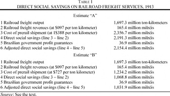
The adjusted nonrail freight charge ranged between 1.388 and 0.727 milréis per ton-kilometer at 1913 prices.
In Table 1 Estimate “A” reveals that the social saving on railroad freight services ran as high as 2.19 billion milréis. The lower half of the table presents Estimate “B,” which puts the resources released to the economy by railroads in 1913 in excess of 1 billion milréis. Both figures are astounding, but warrant a further adjustment. Due to rate regulation the railroad freight charge in 1913 may not represent the full cost of service. Both calculations in Table 1 deduct capital subsidies from the gross benefits. Dividend guarantees disbursed in 1913 were as much as 11.8 million milréis.28
Direct subsidy payments in 1913 were estimated at somewhere between 8.8 and 11.8 million milréis; Ministério da Fazenda, Balanç, table 135; and MVOP, Relatório 1913, p. 21.
Government also paid 16.2 million milréis in interest on loans used to buy up railroads and build new ones. These payments comprised fixed charges not reflected in the freight revenues. Allowing for approximately 9 million milréis in railroad-related loan amortization, the value of the “missing” capital costs comes to 36.9 million milréis, which are deducted from the social savings in
Table 1.
29 The adjustment comes on top of assumptions that already bias downward the unit savings. Charging all of the capital costs against freight services overstates the extent to which railroad freight charges departed from true costs by ignoring other categories of service.
Estimate “A” of the social savings equals nearly 38 percent of Brazilian GDP in 1913, and estimate “B” exceeds 18 percent of GDP.
30 The social-savings estimates here retire the preliminary figures first presented in Summerhill, “Transport Improvements,” pp. 104–08. GDP in 1913 was 5.71 billion milréis; Haddad, “Crescimento Econômico,” pp. 21–41.
These estimates bracket a least-upper bound on the freight social savings. Given that the direct impact appears large, a lower-bound estimate is warranted. The social saving computed on the full level of 1913 service includes savings on a portion of freight whose very existence depended on the role played by the railroad in attracting new resources during the preceding six decades.31
The mixing of direct and indirect effects violates the assumption that the economy's stock of resources was fixed. Adjusting the social saving to a lower bound based on the elasticity of freight demand provides a crude but likely quite effective remedy.
By fixing railroad output at 1.7 billion ton-kilometers, the estimates of
Table 1 assume that the same level of freight service would have been demanded, and produced, at the much higher prerail freight charges. The more likely scenario is that fewer goods would have gone to market, margins of feasible cultivation would be reduced, and manufacturers would stay closer to the coast. The demand for freight services would be lower than it actually was in 1913, and the social savings would be smaller.
How much smaller the social savings would be depends on the sensitivity of demand for freight service to changes in the price of transport. Freight demand elasticities vary considerably across commodities and distance of haul.32
Winston, “Conceptual Developments,” pp. 73–76; Oum, et al., “Concepts,” pp. 151–52; Friedlander and Spady, “Derived Demand Function,” p. 439; and Wilson, “Notes,” p. 13.
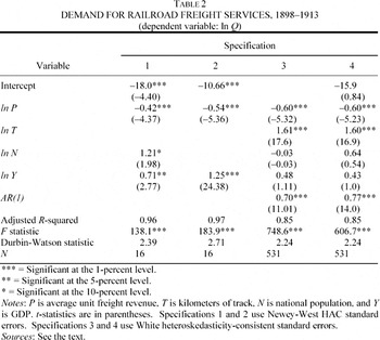
presents an econometric analysis of the market for freight services from 1898 through 1913, using both time series aggregates and an unbalanced panel of cross-section time-series data for 50 railroad lines. With parameter estimates on the price variable falling in the range from −0.42 to −0.60, each specification indicates inelastic demand.
33 The first two specifications use annual time-series aggregates. The first regresses the level of service on the unit charge and GDP. The second specification relies on two-stage least squares estimation to allow for endogeneity of the unit charge, employing track, the price of coal, and a time trend as instruments. The third and fourth specifications use unbalanced panel data on output, price, and track in service for 50 railroad lines and branches, along with common series for GDP and population. The third regression employs fixed effects estimation to accommodate unobservable heterogeneity among the railroads. The fourth specification leaves fixed effects aside, with little difference in the resulting parameters. AR1 estimation is used in the third and fourth specifications to correct for serial correlation. Aggregate figures for track, freight output, and unit freight charges from Summerhill, Order, tables 3.1, 4.4, and 4.6. Time series for GDP and population from Contador and Haddad, “Produto Real,” p. 432. Unit price of coal derived from CPEF, Relatório, 1898–1913, and deflated by the Rio WPI. Line-specific panel data taken from MVOP, Estatísticas, 1898–1913.
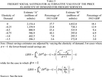
Adjustments to the upper-bound social saving for nonzero values of the price elasticity of demand appear in Table 3. For any elasticity between 0 and −1, Brazil's lower-bound freight social savings exceed upper-bound estimates for most of the advanced industrial economies.34
Upper-bound freight estimates for advanced economies range between 2.5 and 7.1 percent of national income; Hawke, Railways, p. 196; Fishlow, American Railroads, pp. 37, 52; Fogel, Railroads, pp. 219–24; Caron, “France,” p. 44; Fremdling, “Germany,” p. 139; and Laffut, “Belgium,” p. 221.
Adjusting the social saving using elasticities in the range of −0.5 to −1.0 gives measures running between 5 and 16 percent of GDP in 1913. Although the magnitude of the social saving measure proves quite sensitive to the price elasticity of demand for freight services, at the midpoint of the elasticity estimates the savings remain considerable, between 8 and 15 percent of GDP in 1913.
Even at the lower bound the social savings imply a large aggregate productivity gain. Between 1885 and 1913 Brazilian GDP rose from some 1.53 billion milréis to 5.68 billion milréis at 1913 prices, an grew from 12.9 million to 23.7 million. In per capita terms the increase in GDP computed on the 1885 population was 1.56 billion milréis, and 2.89 billion milréis when calculated on the 1913 population. The understated lower-bound “B” estimate of the social saving (evaluated at a price elasticity of demand of −1.0) ran between 10 percent and 19 percent of this productivity gain, and more than 7 percent of the overall increase in GDP. The upper-bound “B” measure accounts for between 36 percent and 66 percent of the increase in output per capita, and almost 25 percent of the change in GDP. Railroad freight services alone accounted for at least 10 percent, and perhaps as much as two-thirds, of Brazil's turn-of-the-century traverse from relative stagnation to economic growth. It is unlikely that any other single technological or institutional innovation in Brazil had so large of an impact before 1914.
PASSENGER SERVICES
Passenger social savings stemmed from the resources released with the shift away from prerail modes of travel. Whereas advanced economies had passenger social savings that accounted for more than one-fifth of the railroad's total direct benefits, in relatively backward economies their contribution was typically more limited.35
In England passenger benefits were at least 28 percent of the total social saving; in France the proportion was 22 percent; in the antebellum United States it was 24 percent and in 1890 it was 28 percent; Hawke, Railways, pp. 40–54; Fishlow, American Railroads, pp. 90–92; Boyd and Walton, “Social Savings,” pp. 237–40; and Caron, “France,” p. 44. Russia came closest among the backward economies to the ratio found in advanced cases, with passenger benefits at 18 percent of total savings. Passenger savings in Spain accounted for 10 to 14 percent of the total direct impact, and for Mexico they were only 5 percent of total gains; Metzer, Economic Aspects, pp. 52–77; Herranz-Loncán, “Railroad Impact,” p. 15; and Coatsworth, Growth, pp. 65–73.
Brazil proves no exception; passenger social savings were small. Brazilians traveled short distances, and the value of the time they saved in traveling by rail was low.
First-class rail travel cost 47 réis per passenger kilometer in 1913, and second-class fares were 26.5 réis.36
Seven railroads accounting for 85 percent of all rail passenger services in 1913 reported first- and second-class revenues that implied average fares of 44 réis and 25 réis, respectively; CM, Relatório; CPEF, Relatório; CSI, Relatório; CB, Relatório; GW, Report; Leopoldina, Report; SP, Report. The fares are low in comparison with those implied by sectoral passenger revenues, and are scaled up by 7 percent to compensate for the difference; MVOP, Estatísticas, 1913, pp. 98–101.
Unit savings on first-class travel fares were large. The alternative to the railroad for first-class travelers was the
diligência (stagecoach). Fares for coach travel in the immediate prerail era were 190 réis per passenger-kilometer in current prices, or some 360 réis in prices of 1913.
37 Rates from CP in the early months of 1865, divided by the contemporary road distance in Müller, São Paulo, map between pp. 244–45, and adjusted to 1913 prices using the extended WPI described previously.
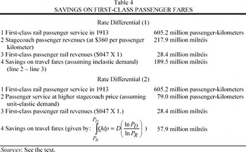
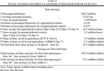
Estimates of the total savings on travel fares for first-class passengers are presented in Table 4. Two cases are considered. The first case assumes that all passengers would have continued to travel in the absence of the railroad. First-class rail service created fare savings of nearly 190 million milréis. However, passenger demand in modern economies is especially sensitive to ticket prices.38
Boyd and Walton, “Social Saving”; and Hawke, “Railway Passenger Traffic,” pp. 367–84.
Stagecoach fares were nearly eight times the prevailing first-class rail charge in 1913. To the extent that travelers considered first-class accommodations a luxury when faced with high stagecoach fares, fewer Brazilians would have opted for such comfort. The second case accommodates this possibility and takes demand for service as unit-elastic with respect to the fare.
39 Unit-elastic demand was assumed for the Netherlands, Russia, and the United States, and is consistent with modern passenger fare elasticities; de Vries, “Barges,” pp. 237–44; Metzer, Economic Aspects, pp. 73–74; Boyd and Walton, “Social Saving”; Winston, “Conceptual Developments,” p. 74; and Owen and Phillips, “Characteristics,” pp. 241, 252.
In this instance the direct savings on first-class tickets come to less than 58 million milréis.
Speed, and not only comfort, distinguished rail passenger travel. Persons not in the work force enjoyed the benefits of the railroad's comfort and security, but the time they saved in traveling by rail had no economic impact, conventionally defined. Rail travelers in the labor force spent less time in transit, which translated into additional savings to the economy. Four assumptions permit a rough estimate of the value of time saved by working first-class rail passengers: stage coaches moved at 13 kilometers per hour40
The speed implied by trip schedules was around 13 kilometers per hour; CP, 20 June 1865; CP, 15 January 1865; Silva, Geographia, p. 90; and Sul de Minas, 30 August 1861.
; passenger trains operated at 39 kilometers per hour
41 Thirty-nine kilometers hour serves as a best guess at the representative passenger train velocity in 1913. Early train speeds varied, from 20 km per hour to 36 km per hour; CP, p. 27 December 1865, p. 2; Estrada de Ferro Leopoldina, Relatório, 1874, p. 2.
; passengers participated in the labor force in the same proportions as the population, so that 34.5 percent of passengers are taken as agricultural workers with another 17.2 percent in nonagricultural occupations
42 IBGE, Estatísticas Históricas, p. 74.
; and first-class travelers in the labor force valued their time at twice the hourly wage in their respective sector of employment.
43 This provides a likely upper-bound on the true value of passenger travel time, based on studies of modern valuation; Winston, “Conceptual Developments,” p. 77; Gronau, Value; De Vany, “Revealed Value,” p. 81; and Beesley, “Value,” p. 182.
In 1913 the average first-class passenger rail journey was 33.05 kilometers.44
Trip length derived from MVOP, Estatísticas, 1913, pp. 98–101, supplemented by passenger statistics for 1913 found in CM, Relatório; CPEF, Relatório; CSI, Relatório; CB, Relatório; GW, Report; Leopoldina, Report; and SP, Report.
Whereas a stagecoach would require 2.5 hours to cover that distance, the same trip was accomplished by rail in slightly less than 50 minutes. Agricultural work paid 179 réis per hour on average, while manufacturing wages ran as high as 1$000 per hour.
45 The average daily wage for farm workers in all of Brazil was 1$609 in 1911; skilled urban manufacturing wages varied, and here are taken at 10$000 per day. Daily wages are converted to hourly rates assuming a 10-hour workday. The wage in agriculture in 1911 is adjusted to 1913 values by the CPI; Brasil, Ministério de Agricultura, Commércio, e Obras Públicas (hereafter MACOP) Aspectos da Economia Rural, under the entries for each state; Oakenfull, Brazil (1913), pp. 564–67.
The time saved by first-class working passengers in
Table 5 came to 16 million hours in 1913. Valued at twice the sectoral hourly wages that time was worth 14.4 million milréis. Combined with the savings on fares, the benefits from first-class rail passenger service equals 72.3 million milréis when demand is taken as unit elastic, and 203.8 million milréis in 1913 with inelastic demand.
46 Whereas fare savings were adjusted to account for elastic demand, no similar treatment extends to the time savings. Given the hypothesis that passenger benefits are small, the assumption merely biases the result upward.
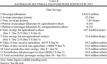
The estimate of second-class passenger savings involves different assumptions. Commercial alternatives to the railroad were prohibitively costly for many.47
The average second-class rail journey in 1913 would have cost more than nine milréis by stagecoach, or nearly a week's earnings in agriculture.
In Brazil's northeast passenger trains operated with a large number of vacancies in the 1870s, yet the dirt roads alongside the tracks were full of travelers.
48 Estrada de Ferro Recife ao São Francisco, Relatório, 1874. For working travelers in second-class it made sense to take the train, because the fare was less than the implied opportunity cost of walking. By the same logic it made sense for travelers not in the labor force to walk.
For second-class passengers the noncommercial alternative to the railroad was either mounted travel or walking. The average second-class railroad trip was only 25.4 kilometers in 1913, which took less than an hour by rail.
49 Calculated from the passenger traffic figures in the sources cited in note 44.
Second-class savings follow from four assumptions: fare savings are negative, because passengers would have walked or ridden in the absence of the train and incurred no outlays; the average speed of foot travel was three kilometers per hour; second-class travelers were in the workforce in the same proportions as the general population; and second-class travelers valued their time at the hourly wage in their respective sectors.
By foot the average second-class railroad trip in 1913 would have required 8.5 hours, and taking the train saved 7.8 hours per passenger trip. Table 6 presents the derivation of the travel time saved on second-class services. Passengers in second class who were classified as “workers” would have saved 161 million working hours, thanks to the higher speed of rail travel. These gross savings were worth 72.8 million milréis to the economy, but only about 46 million milréis once outlays on fares are subtracted.
Total passenger savings in Brazil were low relative to the gains on freight services. With unit-elastic demand, first-class rail passenger services saved only about 1.3 percent of GDP in travel charges and working time in 1913. Under inelastic demand, which is the less likely scenario, the combined fare and travel-time savings rise to 3.6 percent of GDP. Second-class passenger services saved less than 1 percent of GDP in 1913.50
In the United States passenger benefits were 2.6 percent of GNP under the assumption of unit-elastic demand (and nearly double that if demand is taken as inelastic), and in England and Wales passenger savings equaled 5.8 percent of GNP (assuming inelastic demand and that all classes of passengers would have traveled by stagecoach). In Mexico passenger savings hovered around 1 percent of GDP, whereas in Russia they were about 1.2 percent of GNP; Boyd and Walton, “Social Saving,” pp. 249–50; Hawke, Railways, p. 49; Coatsworth, Growth, pp. 71–72; and Metzer, Economic Aspects, pp. 75–76.
Without the railroad, labor markets would have been less integrated, direct fare outlays would have been higher for those traveling commercially, and first-class travelers would have been worse off in pecuniary terms.
51 Between 1890 and 1930 interregional movements of the population come in response to shifting fortunes. The main exception was the increasingly impoverished northeast, which experienced little net migration; Merrick and Graham, “População,” pp. 57–58.
If deprived of its railroad passenger services in 1913 Brazil would have lost a portion of income equal to about two weeks' worth of GDP. A foreign commercial envoy commented in the 1880s on the torpor of travel in Brazil's prerail regions, noting “The axiom ‘Time is Money’ did not yet embody a truth.”
52 Most people had plenty of time but precious little money, and modes of conveyance requiring large cash expenditures were simply beyond their reach.
RETURNS TO RAILROAD INVESTMENT
That Brazilian railroads created a large positive aggregate impact does not necessarily mean they were worth what they cost. Big social savings do not automatically translate into high social rates of return.53
Fogel “Notes,” pp. 12–13.
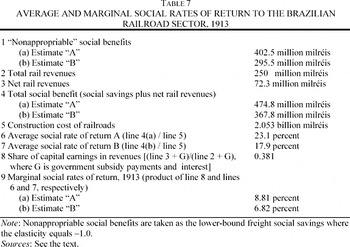
presents estimates of the average social rate of return on two billion milréis invested in Brazil's railroad sector through 1913.
54 Construction costs derived on a line-by-line basis from official statistics and company reports; MVOP, Estatísticas, 1913, pp. 2–11.
The figures ignore passenger benefits altogether, and sum the lower-bound freight social savings from
Table 3 with net operating revenues. Construction costs provide the denominator in the calculation.
55 Reported costs may exaggerate resource costs, as railroad promoters concerned about expropriation could take profits early by padding construction charges; Keefer, “Protection,” pp. 170–92. If construction costs were overstated to the extent they were in Spain, Brazil's average social rates of return would be higher by 50 percent of the estimates here.
Though the private rate of return was a modest 5.32 percent in 1913, the average
social rate of return ran higher, between 17.9 percent and 23.1 percent.
56 Annual average social rates of return on the largest railroads from their earliest operation through 1913 bolster the aggregate finding for a single year here; Summerhill, “Market Intervention.”
These figures are truly astonishing, as they rely only on a lower-bound estimate of freight social savings summed with a modest operating surplus.
57 McClelland, “Social Rates of Return,” p. 485. The social return to railroads in the United States in 1859 and 1890, and England and Wales from 1840 to 1870, ranged between 15 and 20 percent, using upper-bound estimates of the social saving. In poorer economies, where the average social return has been estimated using lower-bound measures, the figure is higher. For Mexico's largest railroad the social return exceeded 20 percent in the 1890s, whereas in Spain it ran between 18 and 23 percent in 1912; Fishlow, American Railroads, pp. 52–55; David, Technical Choice, pp. 310–11; Hawke, Railways, pp. 405–07; Coatsworth, “Impact,” p. 141; and Herranz-Locán, “Railroad Impact,” pp. 16–17.
Had the upper-bound measure of the social saving been used instead, as in the case studies of the United States and England, Brazil's average social rate of return would increase spectacularly, to somewhere between 54 percent and 108 percent.
Whatever manner one chooses to adjust the social savings, the lower-bound average social return suffices to show that Brazil received benefits that justified its investments in the sector. The average return does not, however, reveal whether “too much” or “too little” had been invested, once the returns on alternative projects are taken into account.58
McClelland, “Social Rates of Return,” passim. For statements that Brazil overinvested in railroads see St. Angel, “British Investment,” p. 13; and Villela and Suzigan, Política do Governo, pp. 389–90. Such claims have until now escaped scrutiny, because earlier empirical work was limited to private rates of return; Fendt, “Investimentos Inglêses”; Ribeiro, “Garantias Ferroviárias”; and Rippy, British Investments, pp. 150–58.
Evaluating the efficiency of Brazil's railroad investment requires estimates of the marginal rate of return, indicating the benefit from an additional milréis invested in the sector. Computation of marginal social returns suffers in practice from long-recognized practical difficulties that complicate the interpretation of results.
59 McClelland, “Social Rates of Return,” pp. 471–88; and David, Technical Choice, pp. 307–14.
ventures an estimate, transforming the average rate into a marginal rate with four assumptions: the railroad sector enjoyed constant returns to scale, proportionality held between the social and private output of the sector, the economy had constant returns and competition throughout, and the share of capital earnings (inclusive of government subsidies) in total revenues equals the elasticity of private output with respect to capital.
60 David, Technical Choice, pp. 307–14. The share of capital earnings equals the capital elasticity only if railroads were a constant-returns-to-scale industry. Though railroads are often assumed to have increasing returns, empirical work suggests that such returns are not to scale per se, but rather to traffic density; Keeler, “Railroad Costs,” p. 207, and Railroads, p. 164.
Applying the elasticity to the average social return gives its marginal counterpart. The bottom portion of
Table 7 reports a marginal social return on railroad investment in the range of 6.8 to 8.8 percent.
When compared with private returns the marginal social return suggests that, if anything, Brazil had too little railroad capacity.61
Capital market efficiency requires that the marginal social return equal the private return. Though such a stringent condition did not likely hold in relatively backward economies, markets in Brazil worked well enough to signal opportunity and scarcity, and capital markets in 1913 were significantly more developed than they had been a half-century earlier.
In 1913 the yield on gold bonds was around 5.1 percent, while earnings-price ratios on stocks and bonds for a sample of publicly traded cotton textile firms ran between 7.0 and 8.5 percent.
62 These bound what can be considered a “normal” return in Brazil in 1913. Gold bonds were a relatively low-risk Brazilian security. The textile industry enjoyed heavy tariff protection, so that private rates of return likely exceeded the marginal social return to capital in manufacturing. Textile figures from Haber, “Efficiency Consequences,” table 4; yields on government debt are end-of-year observations in Investors Monthly Manual.
Given the range of these returns, it was highly unlikely that Brazil had over-invested in railroads in the aggregate. The railroad's average social return, and the more conjectural estimates of the marginal social return, equaled or exceeded the market rates of return in other activities, and the private rate of return on the railroad sector itself. Because any loosening of the restrictions applied to the freight social saving would quickly elevate the marginal return into double digits, the results indicate too little railroad investment, rather than too much.
Table 7 nonetheless obscures considerable variation at the subsectoral level by treating the railroad sector as a single, indivisible project. Scrutiny of the marginal social rate of return for individual railroads revealed that many smaller lines did not generate benefits sufficient to justify the investment they made and the subsidies they received.63
The culprits were a number of smaller lines scattered across areas with limited prospects for development. High-return lines were generally, though not exclusively, located in the center-south; Summerhill, “Market Intervention,” and “Institutional Determinants.”
Had government supported railroads where prospects most warranted them, the technology's contribution to national income would have been higher still. That Brazil failed to exploit the full potential of the railroad capital it did attract implicates the policies that promoted particular projects with little merit. The political economics of subsidy led to too much railroad investment in unproductive areas, and too little in more promising regions.
THE FOREIGN AND DOMESTIC CHARACTER OF LINKAGES
Indirect effects, cast in the language of linkages, ran forward and backward from the railroad to the rest of the economy. Backward linkages rested first with the capacity of the railroad's input requirements to stimulate new production. Forward linkages depended mainly on the railroad's potential to generate additional increments of output by attracting mobile factors of production.
The arrival of the railroad in regions where high transport costs had previously circumscribed the feasible margins of cultivation created an expanding agricultural frontier in the latter decades of the nineteenth century. Beginning in the 1880s immigrants poured into São Paulo along with the temperate, fertile states to the south, where the degree of railroad density was among the greatest in Brazil.64
Annual average immigration to São Paulo exceeded 50,000 persons between 1885 and 1913; Holloway, Immigrants, pp. 56–57, 179–81.
New investment attracted by expanding markets boosted capital formation and output in agriculture and industry. Coffee groves in São Paulo multiplied four fold between 1886 and 1915, Brazil's annual imports of industrial machinery quintupled, and textile capacity jumped nearly 20 fold over the same interval.
65 Ibid., p. 178; Suzigan, Indústria Brasileira, pp. 78, 358–61; and Haber, “Efficiency Consequences,” table 6. By 1908 roughly half of Brazil's textile output came from inland factories that depended on railroad transportation; Centro Industrial do Brasil, Brasil, “Mappas Estatísticas,” pp. 1–139; locations based on maps in Mello and Mello, Atlas do Brazil.
The portion of this expansion strictly attributable to the railroad cannot be isolated; by all qualitative indications it was large.
66 Assessments of the forward linkage in a dynamic framework reveal that even modest direct social savings can be associated with very large induced effects; Williamson, Late-Nineteenth-Century American Development, pp. 184–201; Kahn, “Use of Complicated Models,” pp. 185–216; and Foreman-Peck, “Railways,” pp. 83–89.
Even if it accounted for only a small share of the newly accumulated factors of production the railroad's forward linkage provided an appreciable addition to national income.
Large savings on the average cost of shipment did not determine the character of the railroad's forward linkages in Brazil. As Robert Fogel noted the social-saving model was not intended to address such structural consequences.67
For Latin American countries the presumed composition of the forward linkage has garnered more attention than its magnitude. A commonplace of Latin American history is that railroads excessively magnified comparative advantage, resulting in a distorted pattern of export-driven growth.
68 A common corollary is that export-led growth is closely associated with a number of unfavorable social and political outcomes in the historical long run.
Brazil proves a surprising exception in this regard. In 1887 the five major enumerated export goods on 29 lines reporting to the central government comprised 35 percent of total freight shipments.
69 These were coffee, sugar, cotton, hides, and tobacco; MACOP, Relatório, 1887, pp. 66–69; Estrada de Ferro Dom Pedro II, Relatório, 1887, and “Estatística das Mercadorias Expedidas.”
By 1913 the share of export freight had fallen by nearly half, to 18 percent of the total tonnage.
70 MVOP, Estatísticas, 1913, pp. 110–13.
Regulated freight rates favored this shift in the composition of freight. Government set rates especially low for agricultural goods produced and consumed domestically. In contrast to Mexico, where railroad freight charges heavily favored exports, Brazilian freight charges discriminated
against export goods.
71 MVOP, Relatório, 1909, pp. 14–64; and Summerhill, “Market Intervention,” pp. 561–64.
Rates on coffee, the leading export, were well above the average unit revenue on all freight. Domestically produced and consumed items, including wheat flour, corn, rice, manioc flour, beans, and potatoes, all had rates that were significantly lower than those charged for most traditional agricultural exports.
Both the structure of freight rates and the changing proportions of commodities carried by the railroads worked in the same direction as shifts in the economy's overall output mix. The export share of GDP diminished at an average rate between 0.7 percent and 1.5 percent per year, at the very time that economic growth was accelerating.72
Export earnings from IBGE, Repertório Estatístico, pp. 68–69; GDP from Contador, “Crescimento”; and Contador and Haddad, “Produto Real.”
The falling share of exports during the traverse to modern economic growth indicated considerable success that was attributable to the rapid rise of the internal sector of the economy. Differentially high rates on export freight subsidized the movement of domestic goods and bolstered the expansion of domestic markets.
The railroad's derived demands in Brazil did not mirror either the intensity or character of the forward linkage. Though backward linkages were generally modest everywhere (with the exception of Germany), advanced industrial economies succeeded uniquely in capturing the bulk of the railroad's demand for inputs by provisioning their railroad sectors domestically.73
Fremdling, “Railroads,” pp. 583–604; and Caron, “France,” pp. 30–37.
Brazil's domestic backward linkages were, in contrast, limited, consisting of logging for fuel, the establishment of maintenance shops, and the eventual assembly of some rolling stock. No iron and steel industry arose to meet most of the railroads' derived demand, and the bulk of inputs came from abroad. Backward linkages that persistently ran overseas constituted, as John Coatsworth first noted in the Mexican case, a direct leakage of payments from the national income stream.
74 Coatsworth, “Indispensable Railroads,” pp. 955–57.
To assess the extent of this leakage in Brazil a different counterfactual is required, one that assumes the railroads could be supplied domestically rather than from abroad. The estimate has two components: repatriated profits, and outlays on capital goods and operating inputs. Profits (including interest) were remitted to holders of debt and equity in foreign-financed lines. Additional interest payments went to holders of bonds issued by the government to finance construction on state-owned lines, along with the turn-of-the-century recapture of unprofitable lines whose concessions carried guaranteed dividends. In 1913 the sum of all overseas railroad dividends and interest was nearly 72 million milréis.75
These figures assume that none of those shares were held in Brazil, which serves simply to insure that leakage is not understated. Derived from Investors Monthly Manual, November 1913; Annex au Moniteur Belge, 18 July 1914, p. 365; and “Quadro de Titulos da Bolsa do Rio de Janeiro,” Jornal do Commércio, 7 December 1913.
The leakage on material input purchases, taking into account coal imports that can be charged to the railroad sector, along with the costs of imported rails, axles, locomotives, and wagons, comes to nearly 104 million milréis.
76 Coal imports were imputed by regressing railroad coal consumption on ton-kilometers of freight service for 41 lines reporting to the central government. Other foreign railroad inputs derived from import figures for 1913; Brasil, MVOP, Estatísticas, 1913; and Brazil, Comércio Exterior, passim.
Together with the overseas capital payments, orders for merchandise created an outflow abroad of almost 176 million milréis.
77 A meaningful estimate of remittances or import consumption by railroad workers is not possible, though in any case this figure would be small. In Mexico these components came to less than 4 percent of the total leakage; Coatsworth, Growth, pp. 143–44.
Total railroad revenues were 250 million milréis in 1913.
78 MVOP, Estatísticas, 1913, table 20; revenue statements for 1913 in CM, Relatório; CP, Relatório; CSI, Relatório; CB, Relatório; GW, Report; Leopoldina, Report; and SP, Report.
The combined value of remitted profits, interest, and imports of material inputs equaled 70.4 percent of railroad revenues, but only 3 percent of GDP in 1913.
79 This figure corrects an error in converting currency units of the GDP series, which understated the share of leakage; Summerhill, Order, pp. 131–33. Although the estimate here is from a year at the very peak of the country's biggest railroad construction boom, leakage still “cost” less than 18 percent of Brazil's export earnings in 1913; IBGE, Repertório Estatístico, p. 69.
The result bears little resemblance to historiographical claims about the net flows of foreign provisioning running against Brazil, particularly when the social saving that these inputs generated is taken into account. Yet even a small direct leakage might have second-order consequences. Overseas resourcing of the railroad sector implied the export of potentially important employment and income effects. If the railroad sector could have been provisioned at home the domestically channeled demand for inputs might have provided a critical impetus for the early development of coal mining, manufacturing, and capital markets. These additional potential gains, which become opportunity costs if they are sacrificed as a result of foreign dependence, might have been larger than the magnitude of the direct leakage suggests.80
This scenario is implied by criticisms of railroads in Latin America. Coatsworth rendered it explicit in the Mexican case; “Indispensable Railroads,” pp. 959–60. In Spain, the only case where the scenario was operationalized, the developmental consequences of a forced course of domestic linkages were thoroughly negative; Gomez Mendoza, Ferrocarriles, pp. 143–54.
Such opportunity costs were small in Brazil, if they existed at all. An import-substituting industrial strategy was not even remotely feasible in the nineteenth century. Crude forge iron was reasonably common, domestic iron ore deposits were known, and a few blast furnaces had appeared by the 1890s. But the main ore deposits were well inland, in Minas Gerais, themselves requiring a lengthy railroad for exploitation. More importantly, Brazil lacked altogether the coking coal required for a modern iron and steel industry.81
Callaghan, “Obstacles,” pp. 34–40. Similar barriers emerged in the nineteenth-century Russian steel industry in the Urals, leading to a shift in production to Ukraine; Blanchard, “Russian Railway Construction,” pp. 107–26.
Had government implemented protectionist strategies to forge backward linkages, railroad development would have likely ground to a halt, institutionalizing backwardness.
INSTITUTIONAL EXTERNALITIES
Brazil's railroads created less palpable benefits and costs that escape conventional notions of linkages. These effects lie beyond the immediate implications of the railroad for national income, comprising institutional externalities that encompassed broader consequences of the railroad for the long-run trajectory of development.
The railroad did not create “export-led” growth in Brazil in the way it did elsewhere in Latin America, but it did promote the expansion of coffee. Nathaniel Leff first noted that the strength of southeastern coffee exports undermined the international competitiveness of northeastern sugar producers by sustaining a high real rate of exchange.82
Leff, “Economic Development,” pp. 243–62. Though Leff's focus was on whether Brazil was an optimal currency area, an array of other barriers also undermined growth in the northeast, and the strength of this particular mechanism is disputed; Denslow, “Origens da Desigualidade,” pp. 65–88; and Wright, “Cotton Competition,” pp. 625–26.
Similar effects were evident in the far south, as traditional exports there foundered from the 1870s onward.
83 Monasterio, “Decadência das Charqueadas,” pp. 5–11.
The concentration of railroads in the coffee-producing center-south contributed to worsening regional disparities. The exchange-rate consequences of export-boosting railroad expansion compounded pre-existing obstacles to the reallocation of labor across regions. The exacerbation of the Dutch disease in the tropical northeast, where one-third of all Brazilians resided in 1913, was related to the industrial revolution's contribution to transport improvement.
84 This negative externality could have been mitigated by any one of several policy measures: pursuing a much weaker exchange rate, establishing a separate currency area for the northeast, or limiting railroad investment in the center-south.
As early as the 1880s railroads provoked recrudescent provincial protectionism. Local barriers to commerce emerged in response to shifting interregional terms of trade across an array of commodities.85
Bezerra, “Política Tributárial”; Melo, Norte Agrário, pp. 247–85; Deveza, “Política Tributária,” pp. 72–73; Correia, Problema Econômico, pp. 31–34; and Chavantes, Congresso das Vias, pp. 143–44.
This phenomenon involved features far removed from the technology embodied in the railroad itself. Where the polity was fragmented by centrifugal regional forces, as in Old Republic Brazil, the gains from cheap transport were partly undermined by the rise of new obstacles intended to protect influential local interests that stood to lose from the creation of more efficient markets.
The salutary role attributed to railroads in the development of financial and securities markets elsewhere had its echo in Brazil.86
These effects have been highlighted in work on advanced economies; Jenks, “Railroads,” pp. 6–11; Caron, “France,” pp. 28–30; and Hawke, Railways, pp. 388–92.
Reliance on overseas investment to build the railroad sector had few, if any, negative effects on the development of the local capital market. Domestic savings were already prominent in both the sovereign debt market and local enterprises. As early as 1880 railroads accounted for 25 percent of total domestic equity issues on stock exchanges in Rio de Janeiro and São Paulo, and by 1900 railroad securities detained a greater share of domestic market capitalization than any other sector of nonbank business investment.
87 Calculated from Haber, “Efficiency Consequences,” table 1.
Government ownership was, in the first instance, no doubt positive. Railroads created a cadre of professional staff, managers, regulators, and planners in the public sector. Yet in the longer term, the experience with direct government railroad intervention quite likely proved negative. Brazil's early and active politicization, on a national scale, of subsidy, regulation, and ownership created important demonstration effects. The potential advantages of relative backwardness, in the Gerschenkronian sense, could not be realized even by a strong Brazilian state when rent-seeking groups and accommodating policymakers channeled resources to projects with large local pecuniary effects that came at the expense of projects with higher social returns. State intervention in railroads increased the returns to lobbying for rent-seeking interventions elsewhere in the economy, including commodity and financial markets, much of which created no conceivable benefits.88
The government's role in the economy expanded appreciably after 1889, and by the second half of the twentieth century Brazil was awash with state-owned enterprises, many of which generated high costs and performed poorly by either private or social criteria; Topik, Political Economy, passim; and Trebat, Brazil's State-Owned Enterprises, pp. 164–74.
To the extent that modern transport technology elicited policies that laid the groundwork for the grossly distorting and dissipating market interventions of the twentieth century, the railroad may be held culpable in the same measure that it created gains.
CONCLUSIONS
Modern economic growth conventionally depends on capital deepening (to include human capital), and increases in total factor productivity. With respect to social overhead capital the two are not unrelated. Investments in railroads represented a purchase of specialization that boosted productivity in the aggregate, as far fewer resources were required to obtain the same level of transport services.89
Fishlow, American Railroads, p. 223; and Metzer, “Railroads,” p. 62.
Given the geographic distribution of its agronomic endowment Brazil never had a readily affordable alternative to overland shipment. The railroad's impact on aggregate productivity thus proved large. Railroads additionally attracted mobile factors of production. Inflows of labor, and the capital formed in new activities, further boosted national income. Railroads did not forge strong backward linkages, which required a higher prerailroad level of development, and resources specific to industry, than Brazil possessed at the onset of its railroad age. Domestic-use activities proved more responsive to lower transport costs than did exports not only because of a higher elasticity of supply, but also because regulation was highly favorable to production for the domestic market.
Impressive as these accomplishments were, railroad-led growth may still be assigned a supporting role in the legacy of lost opportunities in the late nineteenth century. A wider-ranging counterfactual treatment of Brazil's transition to growth would take into account the entire menu of potential social overhead projects, ranked by their relative returns. Awarding public subsidies to the highest-return projects would doubtless have created a more productive stock of social overhead capital. Near the top of the list would likely be projects known to generate high returns elsewhere, such as subsidies to public education.90
The proportion of people in school in Brazil at the end of the nineteenth century was dismally low, along with the literate share of the population, making it one of the worst cases in the western hemisphere; Mariscal and Sokoloff, “Schooling,” pp. 176–79.
Though railroad technology in the aggregate positioned Brazil for improved economic growth after 1900, the persistent neglect of other forms of social overhead investment (using Hirschman's broader definition) meant that Brazil was not well positioned for the human capital century.
91 Becker, Human Capital, pp. 23–25, 363–48; and Goldin, “Human Capital Century.”
In such a setting the policies that supported projects exhibiting poor social returns merely exacerbated other long-standing obstacles to growth. Considered in light of unrealized complementarities between infrastructure and other forms of social overhead investment, such as even modest increases in human capital, subsidies to low-return rail lines implied considerable opportunities foregone.
The costs of Brazilian subsidy policies in terms of neglected forms of social overhead capital can presently only be guessed at. Assessments will require bridging the divide between nomothetic and ideographic counterfactuals, and between static and dynamic frameworks of analysis. There can be little doubt that the failure to exploit unrealized gains, both within the transport sector and on other types social overhead capital, meant that railroad-led growth proceeded without remedying a highly skewed distribution of income and opportunity.92
The only systematic study of Brazilian inequality during the transition to growth finds improving wealth distribution from 1870 to 1900, but sharply worsening distribution thereafter; Silveira, “Distribution of Wealth,” p. 112.
Such features of Brazilian history direct investigators' attention to the full array of obstacles to development, more broadly defined. Specifying those obstacles and measuring their costs necessarily will draw on the conceptual and empirical rigor that has defined assessments of the impact of railroads in both advanced and backward economies.