2. Theoretical considerations

Darisse, Lemay & Benaissa (Reference Darisse, Lemay and Benaissa2015) have recently carried out extensive measurements in a slightly heated turbulent round jet, and provided the budgets for the transport equations of $k$ , the Reynolds stresses and ${\it\theta}^{\prime 2}$ (the passive temperature variance). These (one-point) budgets, in particular those of $k$ and ${\it\theta}^{\prime 2}$ , are important in the context of s.b.s. budgets. Indeed, the budgets of $k$ and ${\it\theta}^{\prime 2}$ must be recovered from the s.b.s. budgets at large scales. Thus, the single-point budgets provide a test for the validity of the s.b.s. budgets and are required when analysis is to be carried out on an s.b.s. basis. Here, we concentrate only on the equation for $\overline{({\it\delta}q)^{2}}$ , the second-order structure function of the kinetic energy, i.e. $({\it\delta}q)^{2}=({\it\delta}u)^{2}+({\it\delta}v)^{2}+({\it\delta}w)^{2}$ (note that $\overline{q^{2}}=2k$ and ${\it\delta}u=u(x,r)-u(x)$ , where $r$ is the separation between two points considered for evaluating ${\it\delta}u$ ; $u$ , $v$ and $w$ are the fluctuating velocity components along the streamwise, radial and azimuthal directions. It should be noted that the axisymmetry applies along the axis so that, e.g., $\overline{v^{2}}=\overline{w^{2}}$ and $\overline{({\it\delta}v)^{2}}=\overline{({\it\delta}w)^{2}}$ ).

Darisse et al. (Reference Darisse, Lemay and Benaissa2015) showed that the energy contributions from the pressure diffusion, turbulent diffusion and molecular diffusion are negligible on the axis of the round jet. It should be stressed that Darisse et al. (Reference Darisse, Lemay and Benaissa2015) estimated the pressure diffusion term using the Lumley model (Lumley Reference Lumley1978). Further, they inferred $\overline{{\it\epsilon}}$ by closing the energy budget for $k$ (i.e.  $\overline{{\it\epsilon}}={\rm\Sigma}T_{k}$ , where $T_{k}$ represents all remaining terms in the equation of $k$ ). The one-point energy budget on the axis of the round jet obtained by Darisse et al. (Reference Darisse, Lemay and Benaissa2015) is commensurate with the following transport equation for $\overline{({\it\delta}q)^{2}}$ (Danaila, Antonia & Burattini Reference Danaila, Antonia and Burattini2004; Burattini et al. Reference Burattini, Antonia and Danaila2005b ):

(2.1) $$\begin{eqnarray}-\overline{({\it\delta}u)({\it\delta}q)^{2}}+2{\it\nu}\frac{\partial \overline{({\it\delta}q)^{2}}}{\partial r}-\frac{U}{r^{2}}\int _{0}^{r}s^{2}\frac{\partial \overline{({\it\delta}q)^{2}}}{\partial x}\,\text{d}s-2\frac{\partial U}{\partial x}\frac{1}{r^{2}}\int _{0}^{r}s^{2}(\overline{({\it\delta}u)^{2}}-\overline{({\it\delta}v)^{2}})\,\text{d}s=\frac{4}{3}\overline{{\it\epsilon}}r,\end{eqnarray}$$

where the contributions from the turbulent diffusion and pressure diffusion are neglected. In (2.1), local isotropy was assumed. The first and second terms on the left-hand side of (2.1) represent the energy transfer and viscous diffusion at scale $r$ , while the third and fourth terms correspond to the contributions from the advection and production mechanisms, respectively. The right-hand side represents the dissipation of the energy at separation $r$ . For convenience, we hereafter drop the variable $x$ . It is easy to show that when $r\rightarrow \infty$ (2.1) becomes

(2.2) $$\begin{eqnarray}-U\frac{\partial k}{\partial x}-\frac{\partial U}{\partial x}(u^{\prime 2}-v^{\prime 2})=\overline{{\it\epsilon}},\end{eqnarray}$$

the one-point transport equation for $k$ . It is then important to stress that any constraint applied to (2.1) at large $r$ must also apply to (2.2). Let us now seek SP requirements for (2.1) by assuming the following SP forms:

(2.3a,b ) $$\begin{eqnarray}\overline{({\it\delta}q)^{2}}=q_{\ast }^{2}(x)f(r^{\ast }),\quad \overline{({\it\delta}u)^{2}}=u_{\ast }^{2}(x)h_{u}(r^{\ast }),\end{eqnarray}$$

(2.4a−c ) $$\begin{eqnarray}\overline{({\it\delta}v)^{2}}=v_{\ast }^{2}(x)h_{v}(r^{\ast }),\quad \overline{({\it\delta}w)^{2}}=w_{\ast }^{2}(x)h_{w}(r^{\ast }),\quad \overline{({\it\delta}u)({\it\delta}q)^{2}}=(uq)_{\ast }(x)g(r^{\ast }),\end{eqnarray}$$

with $r^{\ast }=r/l_{q}$ ; $l_{q}$ , $q_{\ast }$ , $u_{\ast }$ , $v_{\ast }$ , $w_{\ast }$ and $(uq)_{\ast }^{1/3}$ are the length and velocity scaling functions to be determined; $f$ , $g$ , $h_{u}$ , $h_{v}$ and $h_{w}$ are dimensionless functions. It should be noted that $\overline{({\it\delta}v)^{2}}=\overline{({\it\delta}w)^{2}}$ on the axis of jet. Let us introduce the mixed skewness increment, $S_{q}(r)(\equiv \overline{({\it\delta}u)({\it\delta}q)^{2}}/[\overline{({\it\delta}u)^{2}}^{1/2}\overline{({\it\delta}q)^{2}}])$ , as an SP controlling parameter; this helps for expressing $\overline{({\it\delta}u)({\it\delta}q)^{2}}$ in terms of $\overline{({\it\delta}q)^{2}}$ . If SP is satisfied, then $S_{q}$ also has the SP form $S_{q}(r)=c_{q}{\it\phi}_{q}(r^{\ast })$ (where $c_{q}$ is, in general, a function of $x$ and ${\it\phi}_{q}(r^{\ast })$ is a function of $r^{\ast }$ ), and we can write $(uq)_{\ast }=c_{q}u_{\ast }q_{\ast }^{2}$ . It should be noted also that since we can express $f$ as

(2.5) $$\begin{eqnarray}f=\frac{u_{\ast }^{2}}{q_{\ast }^{2}}h_{u}+\frac{v_{\ast }^{2}}{q_{\ast }^{2}}h_{v}+\frac{w_{\ast }^{2}}{q_{\ast }^{2}}h_{w},\end{eqnarray}$$

and it is independent of $x$ , we must have $q_{\ast }^{2}\sim u_{\ast }^{2}\sim v_{\ast }^{2}\sim w_{\ast }^{2}$ if SP holds. Thus, we can take $u_{\ast }=v_{\ast }=w_{\ast }$ without loss of generality. Substituting (2.3a,b ), (2.4a−c ) and the definition of $S_{q}(r)$ into (2.1) leads to

(2.6) $$\begin{eqnarray}-c_{q}\frac{u_{\ast }l_{q}}{{\it\nu}}G(r^{\ast })+2f^{\prime }(r^{\ast })-\frac{Ul_{q}^{2}}{{\it\nu}u_{\ast }^{2}}\frac{\partial u_{\ast }^{2}}{\partial x}\frac{{\it\Gamma}_{1}}{r^{\ast 2}}+\frac{Ul_{q}}{{\it\nu}}\frac{\partial l_{q}}{\partial x}\frac{{\it\Gamma}_{2}}{r^{\ast 2}}-2\frac{l_{q}^{2}}{{\it\nu}}\frac{\partial U}{\partial x}\frac{{\it\Gamma}_{3}}{r^{\ast 2}}=\frac{4}{3}\frac{\overline{{\it\epsilon}}l_{q}^{2}}{{\it\nu}u_{\ast }^{2}}r^{\ast },\end{eqnarray}$$

with

(2.7) $$\begin{eqnarray}G(r^{\ast })=f(r^{\ast })h_{u}^{1/2}(r^{\ast }){\it\phi}_{q}(r^{\ast }),\end{eqnarray}$$

(2.8a,b ) $$\begin{eqnarray}{\it\Gamma}_{1}=\int _{0}^{r^{\ast }}s^{\ast 2}f(s^{\ast })\,\text{d}s^{\ast },\quad {\it\Gamma}_{2}=\int _{0}^{r^{\ast }}s^{\ast 3}f^{\prime }(s^{\ast })\,\text{d}s^{\ast },\end{eqnarray}$$

(2.8c ) $$\begin{eqnarray}{\it\Gamma}_{3}=\int _{0}^{r^{\ast }}s^{\ast 2}(h_{u}(s^{\ast })-h_{v}(s^{\ast }))\,\text{d}s^{\ast },\end{eqnarray}$$

where $s^{\ast }$ is a dummy variable of integration. Equation (2.6) holds at all scales if ${\it\Gamma}_{1}\sim r^{\ast 3}$ , ${\it\Gamma}_{2}\sim r^{\ast 3}$ and ${\it\Gamma}_{3}\sim r^{\ast 3}$ when $r^{\ast }\rightarrow \infty$ . Since $f(r^{\ast })$ , $h_{u}(r^{\ast })$ and $h_{v}(r^{\ast })\rightarrow \text{constant}$ and $f^{\prime }(r^{\ast })\rightarrow 0$ when $r^{\ast }\rightarrow \infty$ , it is easy to show that these conditions are satisfied. It should be noted also that experimental and numerical evidence shows that when $r^{\ast }\rightarrow 0$ , $f\sim r^{\ast 2}$ . Thus, ${\it\Gamma}_{1}\sim r^{\ast 5}$ (likewise for ${\it\Gamma}_{3}$ ) and ${\it\Gamma}_{2}\sim r^{\ast 5}$ and approach zero more rapidly than $r^{\ast 2}$ .

Self-preservation implies that all coefficients

(2.9) $$\begin{eqnarray}\displaystyle & c_{q}R_{l_{q}}=C_{1}, & \displaystyle\end{eqnarray}$$

(2.10) $$\begin{eqnarray}\displaystyle & \displaystyle \frac{Ul_{q}^{2}}{{\it\nu}u_{\ast }^{2}}\frac{\partial u_{\ast }^{2}}{\partial x}=C_{2}, & \displaystyle\end{eqnarray}$$

(2.11) $$\begin{eqnarray}\displaystyle & \displaystyle \frac{Ul_{q}}{{\it\nu}}\frac{\partial l_{q}}{\partial x}=C_{3}, & \displaystyle\end{eqnarray}$$

(2.12) $$\begin{eqnarray}\displaystyle & \displaystyle \frac{l_{q}^{2}}{{\it\nu}}\frac{\partial U}{\partial x}=C_{4}, & \displaystyle\end{eqnarray}$$

(2.13) $$\begin{eqnarray}\displaystyle & \displaystyle \frac{\overline{{\it\epsilon}}l_{q}^{2}}{{\it\nu}u_{\ast }^{2}}=C_{5}, & \displaystyle\end{eqnarray}$$

where $R_{l_{q}}=u_{\ast }l_{q}/{\it\nu}$ is a scaling Reynolds number, are independent of $x$ , since the coefficient of the second term in (2.6) is a constant. Taking the ratio $C_{2}/C_{4}$ leads to

(2.14) $$\begin{eqnarray}\frac{1}{u_{\ast }^{2}}\frac{\partial u_{\ast }^{2}}{\partial x}\left/\frac{1}{U}\right.\frac{\partial U}{\partial x}=C_{2}/C_{4},\end{eqnarray}$$

which after solving (2.14) yields

(2.15) $$\begin{eqnarray}u_{\ast }^{2}\sim U^{C_{2}/C_{4}}.\end{eqnarray}$$

Forming the sum $(2C_{3}+C_{4})$ and solving leads to

(2.16) $$\begin{eqnarray}l_{q}^{2}U=C_{6}{\it\nu}(x-x_{o}),\end{eqnarray}$$

with $C_{6}=2C_{3}+C_{4}$ . Combining (2.10) and (2.16) and solving yields

(2.17) $$\begin{eqnarray}u_{\ast }^{2}\sim (x-x_{o})^{n},\end{eqnarray}$$

where $n=C_{2}/C_{6}$ . Further, using (2.12) we have

(2.18) $$\begin{eqnarray}U\sim (x-x_{o})^{C_{4}/C_{6}}.\end{eqnarray}$$

Now, we write (2.10) as

(2.19) $$\begin{eqnarray}C_{2}=C_{6}(x-x_{o})\frac{1}{u_{\ast }^{2}}\frac{\partial u_{\ast }^{2}}{\partial x},\end{eqnarray}$$

or equivalently

(2.20) $$\begin{eqnarray}C_{2}=2C_{6}(x-x_{o})\frac{1}{u_{\ast }}\frac{\partial u_{\ast }}{\partial x}.\end{eqnarray}$$

Now, we use the definition of $R_{l_{q}}$ to express $u_{\ast }$ in terms of $l_{q}$ and $R_{l_{q}}$ . This expression is then substituted into (2.20) and together with (2.11) and (2.16) we obtain, after some trivial manipulations,

(2.21) $$\begin{eqnarray}n=\frac{C_{2}}{C_{6}}=-2\frac{C_{3}}{C_{6}}+2(x-x_{o})\frac{1}{R_{l_{q}}}\frac{\partial R_{l_{q}}}{\partial x}.\end{eqnarray}$$

Interestingly, this expression is similar to that obtained by Djenidi & Antonia (Reference Djenidi and Antonia2015) with $C_{3}/C_{6}=1/2$ for homogeneous isotropic decaying turbulence. Since $n$ is a constant, then the second term on the right-hand side of (2.21) must be a constant for any $(x-x_{o})$ . This can occur only when $R_{l_{q}}=\text{constant}$ (which would imply that $c_{q}$ is also constant, according to (2.9)). Accordingly, $n=-2(C_{3}/C_{6})$ , leading to $C_{2}=-2C_{3}$ . Thus, we now have $C_{6}=-C_{2}+C_{4}$ , which yields $1=-(C_{2}/C_{6})+(C_{4}/C_{6})$ . From a dimensional viewpoint, expressions (2.15), (2.17) and (2.18) lead to $C_{2}/C_{6}=2C_{4}/C_{6}$ , thus yielding $C_{4}/C_{6}=-1$ , which leads to $n=-2$ . Finally, we have the SP solutions

(2.22) $$\begin{eqnarray}\displaystyle & \displaystyle U\sim (x-x_{o})^{-1}, & \displaystyle\end{eqnarray}$$

(2.23) $$\begin{eqnarray}\displaystyle & \displaystyle u_{\ast }^{2}\sim (x-x_{o})^{-2}, & \displaystyle\end{eqnarray}$$

(2.24) $$\begin{eqnarray}\displaystyle & \displaystyle l_{q}\sim (x-x_{o}) & \displaystyle\end{eqnarray}$$

(2.25) $$\begin{eqnarray}\overline{{\it\epsilon}}\sim (x-x_{o})^{-4}.\end{eqnarray}$$

We immediately observe that one SP condition imposed on the mean flow is that $U$ must vary like $x^{-1}$ . It should be noted also that since the above conditions apply at all separations for complete SP, then (2.2) also obeys SP and we must have

(2.26) $$\begin{eqnarray}k\sim (x-x_{o})^{-2}\end{eqnarray}$$

(since $k=\overline{({\it\delta}q)^{2}}/4$ as $r\rightarrow \infty$ ). This is the same result as obtained by Thiesset et al. (Reference Thiesset, Antonia and Djenidi2014), who substituted (2.22) (based on the constraint imposed by the mean momentum equation) and (2.25) into (2.2), which in effect is (2.1) at large $r$ . The remarkable feature here is that the decay rates of $U$ and $k$ are derived without explicitly invoking the conservation equations for mean momentum and mean turbulent kinetic energy. In particular, it is the first time that (2.22) is shown to be an outcome, i.e. an SP solution of the s.b.s. budget, rather than an a priori known input. The fact that $U\sim (x-x_{0})^{-1}$ can be derived from the s.b.s. analysis certainly implies that it is also an SP requirement for the mean momentum equation, because the Navier–Stokes equations are the expressions of the conservation of the instantaneous momentum.

One final comment relates to the ‘constant’ $C_{{\it\epsilon}}$ . The $-4$ power law (2.25) was derived without any reference to $C_{{\it\epsilon}}$ . However, we can assess how $C_{{\it\epsilon}}$ must behave when SP is complete. In this case, $L_{u}\sim (x-x_{o})$ and $u^{\prime }\sim (x-x_{o})^{-1}$ , and since also $\overline{{\it\epsilon}}\sim (x-x_{o})^{-4}$ , then $C_{{\it\epsilon}}$ must be constant, regardless of the magnitude of the Taylor microscale Reynolds number $Re_{{\it\lambda}}$ ( $\equiv \,u^{\prime }{\it\lambda}/{\it\nu}$ ; a prime represents the r.m.s. and ${\it\lambda}=(u^{\prime 2}/\overline{(\partial u/\partial x)^{2}})^{1/2}$ is the Taylor microscale). The Taylor microscale Reynolds number $Re_{{\it\lambda}}$ must also be constant in order to satisfy SP.

3. Experimental validation

In this section we present measurements carried out on the centreline of a turbulent round jet with the aim of testing the SP solutions (2.22)–(2.26).

3.1. Experimental facility

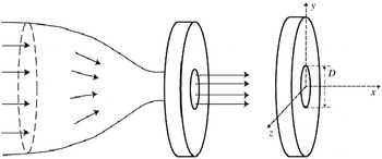
The turbulent jet is generated by an open-circuit wind tunnel. A contraction is attached to the tunnel exit with an area contraction of $85:1$ . The jet exits through a nozzle with a diameter of $D=55~\text{mm}$ (see figure 1). A circular plate of diameter 100 mm is mounted at the nozzle exit and flush with the nozzle exit section to improve the jet flow at the exit, which has a top-hat velocity profile; the incoming boundary layer at the nozzle lip is laminar, although not quite Blasius. The Reynolds numbers $Re_{D}$ , based on the exit velocity $U_{j}$ and $D$ , is varied from approximately 10 000 to 100 000. The velocity is measured with a single hot-wire etched from Wollaston (Pt–10 % Rh) wire to a diameter of $d_{w}=1.2~{\rm\mu}\text{m}$ (which is half the size used by Burattini et al. (Reference Burattini, Antonia and Danaila2005a ,Reference Burattini, Antonia and Danaila b )), and the active length $l_{w}$ is chosen so that $l_{w}/d_{w}$ is nearly $200$ . The ratio $l_{w}/{\it\eta}$ ( ${\it\eta}$ is the Kolmogorov length scale) varies from approximately 5 at $x/D=10$ to 0.87 at $x/D=75$ for the largest Reynolds number. Further details on the experimental set-up can be found in Burattini et al. (Reference Burattini, Antonia and Danaila2005b ).

Figure 1.

Sketch of the jet nozzle and the circular plate.

Hot-wire velocity measurements in turbulent flows may lead to various problems if care is not taken. One such problem relates to the use of Taylor’s hypothesis to convert temporal statistics to spatial statistics. This hypothesis is acceptable when the relative turbulence intensity, $u^{\prime }/U$ , is small. In this case, the convection velocity is assumed to be constant and equal to the mean velocity. In the far field of an axisymmetric jet, the turbulence intensity is approximately 25 % (Mi et al. 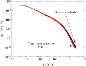Reference Mi, Xu and Zhou2013) which can lead to non-negligible errors in various turbulence statistics. To remedy this problem, in the present work, we applied a correction to the instantaneous velocity signal. A modified version of Taylor’s hypothesis (MTH) has been used based on the method implemented by Kahalerras et al. (Reference Kahalerras, Malecot, Gagne and Castaing1998). The effect of the spatial correction is significant on the statistics of the velocity fluctuations, such as the 1D energy spectrum of $u$ shown in figure 2 and discussed by Burattini et al. (Reference Burattini, Antonia and Danaila2005b ). The major effects of the MTH are concentrated at the high wavenumbers of the spectrum, i.e. at the small scales. The figure shows that the MTH helps to minimise the ‘artificial energy’ added at the high wavenumbers when the ‘standard’ Taylor hypothesis is used. In the context of this work, the application of the MTH is essential for calculating turbulent quantities accurately, such as $\overline{{\it\epsilon}}$ , where the high-wavenumber range of the spectrum is critical.

Figure 2.

The effect of Taylor’s hypothesis on the velocity field. Velocity spectra in the axisymmetric jet ( $Re_{{\it\lambda}}=420$ ).

Figure 3.

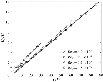
Axial variation of $U^{-1}$ versus $x/D$ for several values of $Re_{D}$ .

Figure 4.

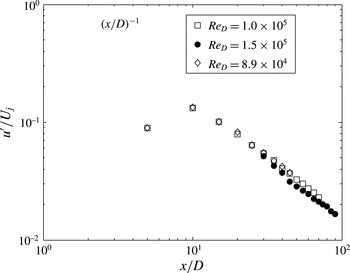
Axial variation of $u^{\prime }$ versus $x/D$ for several values of $Re_{D}$ .

Figure 5.

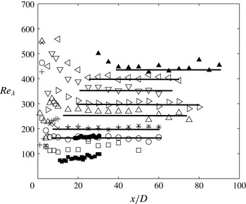
Axial variation of $Re_{{\it\lambda}}$ versus $x/D$ . Present data from bottom to top: $Re_{D}=1\times 10^{4}$ , $2\times 10^{4}$ , $3.4\times 10^{4}$ , $5.3\times 10^{4}$ , $7\times 10^{4}$ , $8.9\times 10^{4}$ and $10\times 10^{4}$ . The horizontal lines are the average values along $x$ , calculated from the streamwise location when $Re_{{\it\lambda}}$ reaches a constant. Mi et al. (Reference Mi, Xu and Zhou2013): ▪, $Re_{D}=1\times 10^{4}$ ; ●, $Re_{D}=2\times 10^{4}$ . Burattini et al. (Reference Burattini, Antonia and Danaila2005b ): ▴, $Re_{D}=13\times 10^{4}$ .

Figure 6.

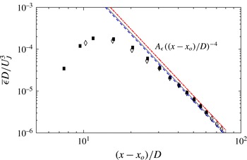
Axial variation of $\overline{{\it\epsilon}}$ versus $x/D$ : ▪, $Re_{D}=8.9\times 10^{4}$ ; ♢, $Re_{D}=1\times 10^{5}$ . The lines are calculated with expression (3.1) where $A_{{\it\epsilon}}=36$ (dashed), 39 (solid) and 48 (dash-dotted) and $x_{o}/D=4.5$ .

3.2. Results

Figures 3 and 4 show the axial variation of the mean velocity and r.m.s. of the longitudinal velocity, $U$ and $u^{\prime }$ respectively; the normalisation is by $U_{j}$ and $D$ . Both distributions comply well with the SP solutions (2.22) and (2.26). The data for $u^{\prime }/U_{j}$ at $Re_{D}=1.5\times 10^{5}$ deviate slightly from the line $(x/D)^{-1}$ in the region 40–60; such a deviation is not discernible in $U$ . We believe that this may be due to some unidentified measurement errors at this particular Reynolds number. The good agreement between the other measured distributions of $u^{\prime }/U_{j}$ and the SP solution (2.26) suggests that SP is complete. This should be reflected in the axial variation of $Re_{{\it\lambda}}$ , which according to SP must be constant. This is indeed observed in figure 5, which shows the centreline evolution of $Re_{{\it\lambda}}$ for several values of the jet Reynolds number $Re_{D}$ . The data of Burattini et al. (Reference Burattini, Antonia and Danaila2005b ) and Mi et al. (Reference Mi, Xu and Zhou2013) are also reported in the figure. It should be noted that for $Re_{D}=1\times 10^{4}$ , $Re_{{\it\lambda}}$ does not appear to be constant, suggesting that SP is not satisfied at this Reynolds number. When $Re_{D}\geqslant 2\times 10^{4}$ , $Re_{{\it\lambda}}$ exhibits a clear plateau over a significant range of $x/D$ . It should be noted though that the beginning of the plateau (i.e. the onset of the SP solutions) moves downstream as $Re_{D}$ increases. For example, SP starts at $x/D\simeq 15$ and 40 when $Re_{D}=3.4\times 10^{4}$ and $13\times 10^{4}$ respectively. The figure clearly reveals that the higher $Re_{D}$ is, the larger $x/D$ should be before SP is reached (or can be observed). For example, when $Re_{D}\geqslant 1\times 10^{5}$ , one needs to carry out measurements beyond $x/D$ of at least 30 before SP occurs. Clearly the constancy of $Re_{{\it\lambda}}$ implies that any length scale, e.g. ${\it\lambda}$ , satisfies (2.24).

To test the SP condition (2.25), we report the centreline variation of $\overline{{\it\epsilon}}D/U_{J}^{3}$ in figure 6 for $Re_{D}=8\times 10^{4}$ and $1\times 10^{5}$ . We used $x_{o}/D=4.5$ as estimated from figure 3. Although not clearly visible on that figure, the straight lines become parallel and intersect the $x$ axis at approximately the same value $x/D=4.5$ , indicating that $x_{o}$ becomes practically independent of the Reynolds number. It should be noted also that since the value of $x/D$ is relatively small in comparison to the extent over which the measurements are taken, a small error in its estimate will not affect the results. Further, $x_{o}$ was also estimated from the distributions of $u^{\prime 2}/U^{2}$ and was found to be approximately $4D$ , in agreement with the estimate obtained from the mean velocity. A comment is required for the estimate of $\overline{{\it\epsilon}}$ . Darisse, Lemay & Benaissa (Reference Darisse, Lemay and Benaissa2014) estimated $\overline{{\it\epsilon}}$ from the balance of the turbulent kinetic energy equation, where the pressure diffusion term was obtained using Lumley’s model (Lumley Reference Lumley1978), while the convection, production, turbulent diffusion and molecular diffusion terms were measured directly. They also showed that $\overline{{\it\epsilon}}_{iso}=15{\it\nu}\overline{(\partial u/\partial x)^{2}}$ , which according to SP can be as expressed by (3.5) which uses local isotropy, is practically equal to $\overline{{\it\epsilon}}$ on the centreline. Further, the fact that the direct numerical simulation of Taub et al. (Reference Taub, Lee, Balachandar and Sherif2013) shows that the pressure term on the centreline is negligible, as predicted by Lumley’s model, provides support for (2.1) on the centreline and gives confidence that $\overline{{\it\epsilon}}\simeq \overline{{\it\epsilon}_{iso}}$ . We thus use $\overline{{\it\epsilon}}_{iso}$ as the surrogate of $\overline{{\it\epsilon}}$ . It should be noted that some justification for identifying $\overline{{\it\epsilon}}$ with $\overline{{\it\epsilon}_{iso}}$ is also provided by previous measurements of all of the components of the dissipation rate for ${\it\theta}^{\prime 2}$ , which seemed to satisfy isotropy reasonably well on the axis of the jet (Antonia & Mi Reference Antonia and Mi1993; Darisse et al. Reference Darisse, Lemay and Benaissa2014). One may find it paradoxical that while local isotropy is not exactly satisfied, $\overline{{\it\epsilon}}$ is approximately equal to $\overline{{\it\epsilon}_{iso}}$ . This is as in grid turbulence, where local isotropy is not verified exactly, but $\overline{{\it\epsilon}}\simeq \overline{{\it\epsilon}_{iso}}$ . The paradox can be explained, at least in grid turbulence where there are compensations among the different terms in the expression of $\overline{{\it\epsilon}}$ (Antonia, Zhou & Zhu Reference Antonia, Zhou and Zhu1998; Djenidi & Antonia Reference Djenidi and Antonia2015), which yield $\overline{{\it\epsilon}}\simeq \overline{{\it\epsilon}_{iso}}$ . We believe that similar compensations occur in the round jet.

When applied to (2.1), the SP analysis shows that $\overline{{\it\epsilon}}$ should vary as $x^{-4}$ on the centreline of the jet. This is well confirmed in the far field of the jet, as illustrated by figure 6. The data shown in this figure are consistent with the data presented in the earlier figures. In particular, the experimental validation of the power law $\overline{{\it\epsilon}}\sim x^{-4}$ confirms that the SP condition $U\sim x^{-1}$ is also experimentally satisfied, as seen in figure 3. Accordingly, and from a theoretical point of view, one must obtain the $-4$ power law when $U\sim x^{-1}$ is used as an input in the SP analysis. This is confirmed by the analysis of Thiesset et al. (Reference Thiesset, Antonia and Djenidi2014) and should be a test of consistency for the measurements. In that regard, the recent experimental results of Sadeghi et al. (Reference Sadeghi, Lavoie and Pollard2015) do not conform with SP requirements. These authors report that $k\sim x^{-1.89}$ and $\overline{{\it\epsilon}}\sim x^{-3.89}$ , which are strictly inconsistent with their observation that $U\sim x^{-1}$ . It should be noted that the $-4$ power-law exponent for $\overline{{\it\epsilon}}$ is obtained if $U\sim x^{-1}$ is based on the SP requirements derived from the theoretical analysis. One of the SP requirements is that $Re_{{\it\lambda}}$ is constant. If this is not verified, one may have $U\sim x^{-1}$ but not the $-4$ power law. This is likely to occur when $Re_{{\it\lambda}}$ is not large enough or the measurements are not acquired at sufficiently large $x/D$ . The measurements of Sadeghi et al. (Reference Sadeghi, Lavoie and Pollard2015) carried out for $Re_{D}=50\,000$ extend only up to approximately $x/D=25$ , which, according to figure 5, is not sufficient for the establishment of SP.

Further experimental validation can be carried out by measuring the prefactor $A_{{\it\epsilon}}$ , whose analytical expression was derived by Thiesset et al. (Reference Thiesset, Antonia and Djenidi2014),

(3.1) $$\begin{eqnarray}A_{{\it\epsilon}}=(2+R)A_{U}^{3}A_{I}^{2},\end{eqnarray}$$

where $A_{U}$ is the prefactor of the power law $U/U_{J}=A_{U}((x-x_{o})/D)^{-1}$ and $A_{I}=(u^{\prime }/U)$ . First, we have obtained (3.1) in a simpler way than Thiesset et al. (Reference Thiesset, Antonia and Djenidi2014), further illustrating that the s.b.s. equation contains all of the dynamics of the flow. Since (2.1) and (2.2) are equivalent at large separations $r$ and SP is complete, we can write (2.2) in its SP form

(3.2) $$\begin{eqnarray}-\left(\frac{U}{U_{J}}\right)\frac{\partial (k/U_{J}^{2})}{\partial (x-x_{o})/D}-\frac{\partial (U/U_{J})}{\partial (x-x_{o})/D}\left(\frac{u^{\prime 2}}{U_{J}^{2}}-\frac{v^{\prime 2}}{U_{J}^{2}}\right)=\frac{\overline{{\it\epsilon}}D}{U_{J}^{3}}.\end{eqnarray}$$

The first term on the left-hand side of (3.2) can be written as

(3.3) $$\begin{eqnarray}A_{u}^{3}A_{I}^{2}(1+2R)\left(\frac{x-x_{o}}{D}\right)^{-4},\end{eqnarray}$$

after using $k=(1/2)(1+2R)u^{\prime 2}$ and $(u^{\prime 2}/U_{J}^{2})=(u^{\prime 2}/U^{2})(U^{2}/U_{J}^{2})=A_{I}^{2}A_{U}^{2}(x-x_{o})D^{-2}$ . Similar manipulations for the second term on the left-hand side of (3.2) yield

(3.4) $$\begin{eqnarray}A_{u}^{3}A_{I}^{2}(1-R)\left(\frac{x-x_{o}}{D}\right)^{-4}.\end{eqnarray}$$

Finally, the summation of (3.3) and (3.4) leads to

(3.5) $$\begin{eqnarray}\frac{\overline{{\it\epsilon}}D}{U_{J}^{3}}=(2+R)A_{u}^{3}A_{I}^{2}\left(\frac{x-x_{o}}{D}\right)^{-4},\end{eqnarray}$$

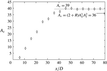
which leads to (3.1) for $A_{{\it\epsilon}}$ . Figure 7 shows that $A_{{\it\epsilon}}$ is constant for $x/D\geqslant 45$ , thus marking the onset of SP on the jet axis. The values shown in figure 7 are obtained by plotting $\overline{{\it\epsilon}}D/U_{J}^{3}((x-x_{o})/D)^{4}$ . The values of $A_{{\it\epsilon}}$ shown in figure 7 and lying on the plateau are approximately 8 % larger than the value inferred from (3.1), where $R$ is $2/3$ (Burattini et al. Reference Burattini, Antonia and Danaila2005b ) and $A_{U}$ and $A_{I}$ , as obtained from the present measurements, are approximately 6 and 0.25 respectively. Interestingly, the value of $A_{{\it\epsilon}}$ proposed by Friehe et al. (Reference Friehe, Atta and Van Gibson1971) is 48 (see also Antonia et al. Reference Antonia, Satyaprakash and Hussain1980), approximately 23 % larger than the present experimental value and approximately 33 % larger than the present predicted value (approximately 36). An analysis of the data of Burattini et al. (Reference Burattini, Antonia and Danaila2005b ) yields an experimental value for $A_{{\it\epsilon}}$ of 42.5 (see Thiesset et al. Reference Thiesset, Antonia and Djenidi2014), not too different from the present value, while Mi et al. (Reference Mi, Xu and Zhou2013) reported a value of approximately 50. Thiesset et al. (Reference Thiesset, Antonia and Djenidi2014) reported values of $A_{{\it\epsilon}}$ calculated with (3.1) using the data of Friehe et al. (Reference Friehe, Atta and Van Gibson1971), Burattini et al. (Reference Burattini, Antonia and Danaila2005b ) and Mi et al. (Reference Mi, Xu and Zhou2013) and obtained 39.7, 32.7 and 33.5 respectively, which are in quite good agreement with our calculated value. Using the data of Darisse et al. (Reference Darisse, Lemay and Benaissa2015), we found that $A_{{\it\epsilon}}=41$ when calculated with (3.1), while the experimental estimate is approximately 42. Finally, using the correction of $\overline{{\it\epsilon}}$ proposed by Darisse et al. (Reference Darisse, Lemay and Benaissa2015), we also calculated $A_{{\it\epsilon}}$ based on (3.1) for the data of Panchapakesan & Lumley (Reference Panchapakesan and Lumley1993) and Hussein, Capp & George (Reference Hussein, Capp and George1994) and found 34.8 and 38.8 respectively. While relatively small, the variation of the analytical values between these experiments is likely to reflect the differences in initial conditions, which certainly affect the experimental estimates of $R$ , $A_{U}$ and $A_{I}$ (e.g. the review of Gouldin et al. (Reference Gouldin, Schefer, Johnson and Kollman1986) shows a large variation in the values of $A_{U}$ and $x_{o}/D$ ; see also the latest review of George (Reference George2012)). To assess (3.1) further, we report in figure 6 the values of $\overline{{\it\epsilon}}D/U_{J}^{3}$ calculated from (3.5) with $A_{{\it\epsilon}}=36$ , 39 and 48 respectively, and $x_{0}=4.5D$ . There is a relatively good match between the measurements and the prediction for $(x-x_{o})/D\geqslant 40$ when $A_{{\it\epsilon}}=36$ (the line corresponding to $A_{{\it\epsilon}}=39$ is shown only as a reference), confirming the validity of expression (3.1) and suggesting that the present value of $A_{{\it\epsilon}}$ is closer to 40 than the value of 48 of Friehe et al. (Reference Friehe, Atta and Van Gibson1971). It should be noted that since the calculation of $A_{{\it\epsilon}}$ involves only statistics whose contributions are mainly from the lower end of the spectrum (i.e. large-scale motion), any error associated with the high-wavenumber range is not critical.

Figure 7.

Axial variation of $A_{{\it\epsilon}}$ versus $x/D$ for $Re_{D}=1\times 10^{5}$ . The value of $A_{{\it\epsilon}}$ inferred from the expression (3.1) is marked by an arrow. The dashed line is used as a visual aid only.

Figure 8.

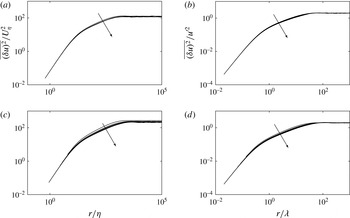
Axial variation of $\overline{({\it\delta}u)^{2}}$ . (a,c) Normalisation with Kolmogorov scaling; (b,d) normalisation with $u^{\prime 2}$ and ${\it\lambda}$ . The arrow is in the direction of increasing $x/D$ from 10 to 60 for $Re=3.4\times 10^{4}$ (a,b) and 10 to 80 for $Re=10\times 10^{4}$ (c,d).

Figure 9.

Axial variation of $-\overline{({\it\delta}u)^{3}}$ . (a,c) Normalisation with Kolmogorov scaling; (b,d) normalisation with $u^{\prime 2}$ and ${\it\lambda}$ . The arrow is in the direction of increasing $x/D$ from 10 to 60 for $Re=3.4\times 10^{4}$ (a,b) and 10 to 80 for $Re=10\times 10^{4}$ (c,d).

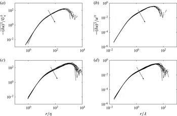
Finally, further evidence of SP can be shown through the second- and third-order structure functions for the longitudinal velocity measured at several positions along the jet axis. If SP is satisfied, the structure functions should collapse regardless of which set of SP scaling variables is used. Figures 8 and 9 show these functions for two Reynolds numbers at various values of $x/D$ . Both normalisations with Kolmogorov scaling variables and with $u^{\prime 2}$ and ${\it\lambda}$ are used. Ignoring the stations over which $Re_{{\it\lambda}}$ is not constant (see figure 5), and regardless of the normalisation, both the second- and third-order structure functions present a good collapse over practically the entire range of $r$ , which is equivalent to a collapse in velocity spectra at all wavenumbers (not shown here; see also Burattini et al. (Reference Burattini, Antonia and Danaila2005a ,Reference Burattini, Antonia and Danaila b )). It should be noted, however, that $x/D$ needs to be sufficiently large before SP applies, and the collapse is somewhat impaired for $\overline{({\it\delta}u)^{3}}$ when $r$ becomes large, i.e. $\overline{({\it\delta}u)^{3}}$ approaches zero.

4. Concluding remarks

A self-preservation (SP) analysis has been applied to the transport equation for the second-order structure function $\overline{({\it\delta}q)^{2}}$ , often referred to as the s.b.s. budget equation (2.1), on the axis of a turbulent round jet. The equation admits the following complete SP solutions, i.e. SP is satisfied at all scales of motion: $R_{l}=\text{constant}$ , $U\sim \sqrt{k}\sim x^{-1}$ , $\overline{{\it\epsilon}}\sim x^{-4}$ , $l\sim x$ . Because SP is complete, any characteristic length, e.g. ${\it\eta}$ ( $=({\it\nu}^{3}/\overline{{\it\epsilon}})^{1/4}$ , the Kolmogorov length scale), ${\it\lambda}$ (Taylor microscale) or jet half-width can be used as a scaling length. Similarly, there are several options for velocity scales, e.g. $U$ , $\sqrt{k}$ and the Kolmogorov velocity ( $v_{K}=({\it\nu}\overline{{\it\epsilon}})^{1/4}$ ). Remarkably, the analysis does not require the ad hoc (additional) use of conservation equations for $U$ and $k$ , underlying that information about the SP behaviour of these quantities is intrinsic to the s.b.s. equations. It should be noted that this is not too surprising in the case of $k$ , since its transport equation is recovered from the s.b.s. equations at large scales. This is less evident for $U$ . In fact, the analysis shows that $U\sim (x-x_{o})^{-1}$ is a solution of the SP analysis applied to the s.b.s. energy budget rather than an input.

The theoretical SP solutions compare very well with both our present and our previous experimental data on the axis in the far field of the round jet. These measurements show that, after a transient downstream distance which increases with the Reynolds number, the turbulence decay on the centreline of the round jet evolves in a manner consistent with complete SP (e.g. $Re_{{\it\lambda}}=\text{constant}$ , $U\sim u^{\prime }\sim x^{-1}$ , $\overline{{\it\epsilon}}\sim x^{-4}$ and ${\it\lambda}\sim x$ ).

The experimental SP evidence presented here on the axis of the round jet gives further support to the work of Thiesset et al. (Reference Thiesset, Antonia and Djenidi2014), who used the SP framework applied to (2.1) when $r\rightarrow 0$ to investigate the transport equation of $\overline{{\it\epsilon}}$ . In particular, it validates the hypotheses they used, i.e. complete SP and the terms retained in (2.1), to carry out the theoretical analysis.

The present analysis on the jet axis should be extended to locations away from the axis of the jet. This requires study of the behaviour of the s.b.s. budget at various $y$ locations. Indeed, this budget is expected to vary with $y$ , reflecting the expected variation with $y$ of the single-point turbulent energy budget. For example, while the contributions from the turbulent diffusion and pressure diffusion are negligible on the axis, they become important away from the axis. Moreover, the assumption of local homogeneity and local isotropy needs to be tested away from the axis.