NOMENCLATURE
- ANN
-
artificial neural networks
- POD
-
projection orthogonal decomposition method
- SVD
-
singular value decomposition
- CFD
-
computational fluid dynamics
- A
-
flow field data matrix
- M h
-
the flow field data dimension
- M s
-
the number of samples
- U,V
-
an orthogonal matrix
- podbasic
-
the number of modal
-
 ${\hat{U}}$
-
podbasic columns of U
-
$\mathbb{R}$
-
real domain
- X
-
input of ANN
- Y
-
output of ANN
-
$\tilde{Y}$
-
the approximation of Y
- W
-
the weight of the output of ANN
- B
-
the bias of ANN
-
$S_i$
-
the solution vector of flow field data
- E
-
function of the squared error


Greek Symbol
-
$\Sigma$
-
singular value matrix
-
$\hat{\Sigma}$
-
podbasic lines of
$\hat{\Sigma}$
-
$\Lambda$
-
equals
$\Sigma V^{T}$
-
$\hat{\Lambda}$
-
podbasic lines of
${\Lambda}$
-
$\Upsilon$
-
energy function
-
$\theta$
-
the activation function
-
$\Xi$
-
parameter set
- Phi
-
the mapping


1.0 INTRODUCTION
Nowadays, multi-dimensional aerodynamic databases have been widely used in design, optimisation, control and other related research fields, which have high research value and practical significance. Among them, multi-dimension represents multiple parameters, such as flying height, Mach number, angle of attack, etc. However, the amount of data required often exponentially increases with the dimension, which we called the curse of dimensionality(Reference Lorente, Vega and Velazquez1). Thus, the multi-dimensional nature will make the calculation amount very large. In order to reduce the computational overhead, data dimension reduction is particularly important. The projection-based dimension reduction method is a relatively common projection method(Reference Hesthaven, Rozza and Stamm2). The most attractive point of this method is that it can save the model structure and ensure the universality of the method. It is especially important for data-based models because the model can be improved in time and applied to hidden conditions that cannot be observed during the model changes. There are two main methods based on projection, including orthogonal decomposition method (POD)(Reference Liang, Lee, Lim, Lin, Lee and Wu3) and greedy algorithm(Reference Hesthaven, Stamm and Zhang4). The POD method requires a sample in a parameter space, then it needs singular value decomposition, and constructs a space that requires less modality, while the greedy algorithm selects samples in an adaptive and minimising error manner(Reference Yu and Hesthaven10). Therefore, the greedy algorithm should be more efficient than the POD algorithm; however, the criteria for sample selection in practical applications are not easy to determine, which leads to greedy algorithms that are not always feasible.
In addition, since the new space constructed based on the projection model uses only a few modals, this method also has significant advantages in terms of computational efficiency. Furthermore, due to the differences in operating platforms and the affine dependence of the right-hand rule, the parameters of the projection model are generally not suitable for general nonlinear problems. Hesthaven et al.(Reference Hesthaven, Stamm and Zhang4) and Sha et al.(Reference Shah, Xing and Triantafyllidis5) proposed an improved POD method, which approximates the nonlinear properties of POD bases and new parameters. This method is not described in detail in this paper. The detailed study on this model can be found in Ref. (Reference Benner, Gugercin and Willcox6).
And in other references, Per Christian Hansen(Reference Hansen37) proposed that the truncated singular value decomposition (SVD) can be considered as a method for regularisation of ill-posed linear least squares problems. And he introduced some basic theory of SVD. Shnayderman, A., Gusev, A. and Eskicioglu, A.M.(Reference Shnayderman, Gusev and Eskicioglu38) introduced the application of the SVD method in image processing. In fact, image processing also means processing the data matrix. Drma and Veseli(Reference Drma and Veseli39) introduced how to break the barrier between numerical accuracy and run-time efficiency in computing the fundamental decomposition of numerical linear algebra — the singular value decomposition (SVD) of general dense matrices. G. Berkooz, P. Holmes and J.L. Lumley(Reference Berkooz, Holmes and Lumley40) introduced the basic theory of the POD method in detail. CW. Rowley(Reference Rowley41) compared three different methods of model reduction: proper orthogonal decomposition (POD), balanced truncation and a method called balanced POD. K. Kunisch and S. Volkwein(Reference Volkwein42) proved error estimates for Galerkin proper orthogonal decomposition (POD) methods for nonlinear parabolic systems arising in fluid dynamics. Y.C. Liang and other authors(Reference Liang, Lee and Lim43) gave a summary of the POD methods and showed the connections among these methods.
In recent years, data-based models have been widely favoured by scholars in various fields. Data-based intelligent learning algorithm (also known as machine learning) has developed rapidly, such as Refs Reference Iungo, Santoni-Ortiz, Abkar, Porté-Agel, Rotea and Leonardi11 and Reference Peherstorfer and Willcox12. Its basic idea is to collect sample data and directly analyse its underlying mechanism. Machine learning methods are widely used in the fields of image processing, speech recognition, drug research, etc., which show great potential for scientific computing in various fields. It is well known that artificial neural network (ANN) is one of the machine learning algorithms. The concept of artificial neural network originates from biology. Neural network consists of simple but interrelated elements called neurons(Reference Tosun, Aydin and Bilgili23). ANNs are usually non-linear and are suitable for a variety of classification and regression problems, and can approximate any linear and nonlinear functions with different complexity(Reference Cybenko24,Reference Cybenko25) . The role of ANN is to form different functional relationships between vectors. As an important non-parametric data-driven model, ANN can make full use of the data and determine the structure and parameters of the model from the data without any restrictions and assumptions. Thus, it can obtain good prediction results.
Computational fluid dynamics, as an important branch of scientific computing, incorporates many machine learning strategies. The field of fluid field remodelling in computational fluid dynamics (CFD) includes turbulence models(Reference Tracey, Duraisamy and Alonso13–Reference Ling, Kurzawski and Templeton16), transition models(Reference Duraisamy, Zhang and Singh17), flow control(Reference Lee, Kim, Babcock and Goodman18), unsteady aerodynamic prediction(Reference Kurtulus19), etc. This paper mainly considers the flow field reconstruction problem (that is to say, reconstructs the flow field from the collected high-precision data samples). Bui-Thanh et al. also did related research work(Reference Bui-Thanh, Damodaran and Willcox20). In addition, Luo Jie et al.(Reference Jie, Yanhui and Jinsheng7) and Qiu Yasong et al.(Reference Yasong, Junqiang and Jun8) also did related research on eigen-to-orthogonal decomposition and discussed in detail the criteria for modal selection of energy and modal numbers in flow places. In these studies, a flow field prediction correlation method based on intrinsic orthogonal decomposition was proposed. Hu Zhi et al.(Reference Zhi, Peng-yin, Xiao-cheng and Zhao-hui9) analysed the dynamic modal decomposition applied to different degrees of dynamic stall flow field, and some scholars proposed a method combining interpolation with improved orthogonal decomposition, etc. The improved orthogonal decomposition is called gappy POD(Reference Everson and Sirovich21) (gappy POD method generates high-precision samples multiple times at the beginning and then interpolates for the parameters sought). After that, gappy POD extended to unsteady flow reconstruction problems(Reference Willcox22) and so on.
In this paper, an array neural network method is proposed based on the flow field reconstruction method, which uses the artificial neural network(Reference Yu and Hesthaven10). We obtain a set of high-precision samples through CFD calculation, which we called the target problem. Then we simplify the problem and reduce the amount of data by POD method. At the same time, we seek to approach the target problem with a certain degree of accuracy. The simplified problem corresponds to the sample of the target problem. Then we hope to use the array neural network to establish a mapping between the flow field features of simplified target problem and the flow field data. We first train the neural network with the known samples. For the unknown flow field data, the trained neural network is used to predict the simplified problem. Finally, we use the reverse POD process to restore the simplified samples to the high-precision samples.
In this paper, we describe the calculation methods in Sections 1 and 2 at first, including POD methods and ANN methods. In the third section of this paper, the flow field reconstruction method based on array neural network is proposed. Then in the fourth section, several typical airflow flow field examples are given, and the figures of calculated reconstruction flow field are shown. What’s more, we analyse the energy of modals. Finally, we give some conclusions in the fifth section.
2.0 POD METHOD
In this section, we describe the POD method. The POD method is actually divided into two parts, singular value decomposition and projection transformation. First, we perform singular value decomposition (SVD) on the sample matrix; then we select the appropriate number of modals for projection. Finally, we obtain the simplified sample data.
2.1 SVD matrix decomposition
Singular value decomposition is an important matrix decomposition in linear algebra and has important applications in signal processing and statistics(Reference Hansen37). Singular value decomposition is similar to the diagonalisation of symmetry matrices or Hermit matrices based on eigenvectors in some respects. However, although these two matrix decompositions are related, they are significantly different. The basis of symmetric vector decomposition is spectral analysis, while singular value decomposition is the generalisation of spectral analysis theory on arbitrary matrices(Reference Shnayderman, Gusev and Eskicioglu38).
SVD.

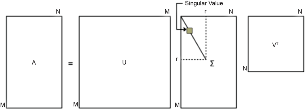
SVD is essentially the decomposition of matrix, which is different from eigendecomposition. SVD doesn’t require that the matrix must be a square matrix(Reference Shnayderman, Gusev and Eskicioglu38). Suppose A is an
 ${M_h} \times {M^s}$
matrix, where
 ${M_h}$
is the flow field data dimension,
 ${M^s}$
is the number of samples, and all of the elements in
 $A$
belong to the domain
 $K$
which is the real or complex domain. Thus, there is a decomposition that makes
 \begin{equation*}A = U\Sigma {V^T} = \mathop \sum \limits_{i=1}^r {\sigma _i}{u_i}v_i^T\end{equation*}
where
 $U$
is an
 ${M_h} \times {M_h}$
orthogonal matrix,
 $\Sigma = diag\!\left( {{\sigma _1}, {\cdots },{\sigma _r}} \right)$
is a matrix of
 ${M_h} \times {M^s}$
, its elements are all zero, except the elements on the main diagonal. On the main diagonal of
 $\Sigma $
each element is a singular value (
 $r \le min\!\left( {{M_h},{M^s}} \right)$
), and
 $V$
is an
 ${M^s} \times {M^s}$
orthogonal matrix.
Figure 1 visually shows the definition of SVD above.
In addition, both
 $U$
and
 $V$
are unitary matrix, which satisfied
 \begin{equation*}{U^T}U = I,{\rm{\ \ }}{V^T}V = I\end{equation*}
Among them, the columns of
 $V$
constitute a series of orthogonal “input” base vectors, which are the feature vectors of
 ${A^T}A$
. We obtain these vectors through matrix operation. First, we multiply
 ${A^T}$
and
 $A$
to obtain a square matrix
 ${A^T}A$
of
 ${M^s} \times {M^s}$
. Since
 ${A^T}A$
is a square matrix. It can perform eigenvalue decomposition, whose feature values and feature vectors satisfy
 \begin{equation*}\!\left( {{A^T}A} \right){v_i} = {\lambda _i}{v_i}\end{equation*}
Thus,
 ${M^s}$
eigenvalues and the corresponding
 ${M^s}$
eigenvectors
 ${v_i}$
of
 ${A^T}A$
are obtained. Then we form all the feature vectors of
 ${A^T}A$
into an
 ${M^s} \times {M^s}$
matrix
 $V$
. Thus, matrix
 $V$
is obtained.
Similarly, the columns of
 $U$
form a set of orthogonal “output” base vectors, which are eigen vectors of
 $A{A^T}$
. The method of getting
 $U$
is similar to V.
The elements on the diagonal of
 $\Sigma $
are singular values that can be thought of as scalar “expansion controls” between input and output(Reference Drma and Veseli39). These elements are the non-negative square roots of the eigenvalues of
 ${A^T}A$
and
 $A{A^T}$
, which correspond to the row vectors of
 $U$
and
 $V$
. We obtain these elements though the method as following
 \begin{align*}A &= U\Sigma {V^T}\\ \Rightarrow AV &= U\Sigma {V^T}V \Rightarrow AV = U\Sigma\\ \Rightarrow A{v_i} &= {\sigma _i}{u_i} \Rightarrow {\sigma _i} = A{v_i}/{u_i}\end{align*}
Then we can obtain the singular value matrix
 $\Sigma $
.
2.2 Projection transformation
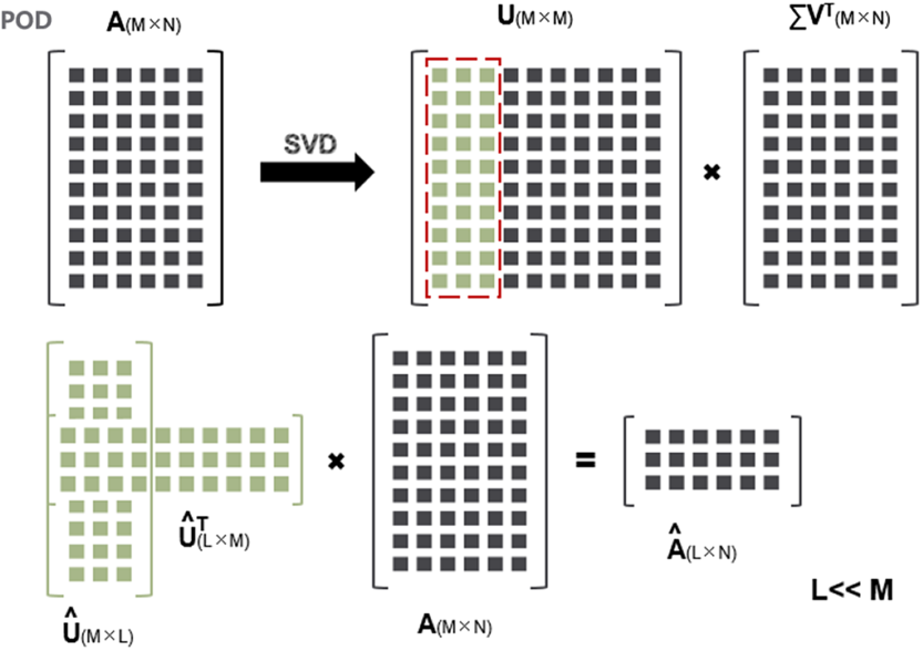
For the convenience of calculation, we multiply
 $\Sigma $
and
 ${V^T}$
, which are among the three matrices obtained by SVD decomposition(Reference Yu and Hesthaven10):
 \begin{equation*}A = U \times \Sigma {V^T} = U{\rm{\Lambda }}\end{equation*}
where
 $\Sigma {V^T}$
is a matrix of
 ${M_h} \times {M^s}$
.
Then we consider the projection transformation(Reference Rowley and Dawson28). Suppose that the number of modal (base) we choose is
 $podbasic$
, that is, we select the
 $podbasic$
lines of
 $\Sigma $
(recorded as
 $\widehat{\Sigma} $
) and multiply it by
 ${V^T}$
, which in order to get the matrix
 $\widehat{\Sigma} {V^T}$
of
 $podbasic \times {M^s}$
(recorded as
 $\hat \Lambda $
). However, for the convenience of the program operation, we choose its equivalent form. We select the first
 $podbasic$
columns of
 $U$
(denoted as
 $\skew2\widehat{U}$
), and left multiply its transposition by matrix
 $A$
. Here, we choose the transposition is because
 $U$
is an orthogonal matrix. There is a theorem can prove that the transposition of an orthogonal matrix is equal to the inverse of an orthogonal matrix(Reference Berkooz, Holmes and Lumley40–Reference Liang, Lee and Lim43). Therefore, taking the transposition is equal to taking the inverse matrix. Finally, we can obtain the equivalent form
 ${\skew2\widehat{U}^T}$
 $A$
of
 $\widehat{\Sigma} {V^T}$
. That is
 \begin{equation*}{U^T}A = \Sigma {V^T} \Rightarrow {\skew2\widehat{U}^T}A = \widehat{\Sigma} {V^T}\end{equation*}
As shown in the following Fig. 2.
POD.

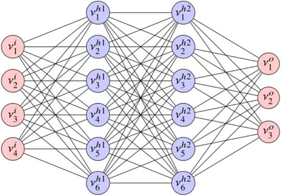
Multi-layer feedforward neural network(Reference Yu and Hesthaven10).

In fact, the value of
 $podbasic$
is determined by the metric
 ${\varepsilon _{POD}}$
 \begin{equation*}{\rm{\Upsilon }}\!\left( {podbasic} \right) = {{\mathop \sum \nolimits_{m=1}^{podbasic} \sigma _m^2} \over {\mathop \sum \nolimits_{m=1}^{{M^s}} \sigma _m^2}} \ge 1 - \varepsilon _{POD}^2\end{equation*}
where
 ${\rm{\Upsilon }}\!\left( {podbasic} \right)$
represents the percentage of energy retained under the modal (base), the number of modal is
 $podbasic$
, we called it the generalised “energy”(Reference Yu and Hesthaven10). If
 $\skew6\hat{A}$
meets the formula above, then we have
 \begin{equation*}{{{{\| {\skew6\hat{A} - A} \|}_F}} \over {{{\left\| A \right\|}_F}}} \le {\varepsilon _{POD}}\end{equation*}
where
 ${\left\| \cdot \right\|_F}$
represents the Frobenius norm.
However, in fact, we only calculate the coefficient matrix
 $\hat \Lambda={\skew2\widehat{U}^T}A$
when we train the ANN.
3.0 ANN METHOD
We choose TensorFlow(Reference Abadi, Barham, Chen, Chen, Davis, Dean, Devin, Ghemawat, Irving, Isard, Kudlur, Levenberg, Monga, Moore, Murray, Steiner, Tucker, Vasudevan, Warden, Wicke, Yu and Zheng29,Reference Glorot, Bordes and Bengio31) as the framework for ANN. Then we briefly introduce the multilayer feed-forward neural network(Reference Karlik and Olgac30) used in this paper, which is most widely used in ANNs. A typical multilayer feed-forward network is shown in Fig. 3. It consists of three types of layers (one input layer, two hidden layers, and one output layer), each layer consists of one or more neurons. Feed-forward means that the information in the neural network flows only from input layer to output layer, instead of reverse (cyclic) propagation. Although it has been demonstrated in article(Reference Taira, Brunton, Dawson, Rowley, Colonius, McKeon, Schmidt, Gordeyev, Theofilis and Ukeiley27) that a neural network containing two hidden layers and a differentiable function is sufficient to approximate any function, there is no definitive rule for determining the number of neurons required for each layer.
Suppose that we know two vectors
 ${\rm{X}} \in {\mathbb{R}^{{N^i}}}$
and
 ${\rm{Y}} \in {\mathbb{R}^{{N^o}}}$
, we seek to establish a mapping between the two vectors:
 $\emptyset $: ${\mathbb{R}^{{N^i}}} \mapsto {\mathbb{R}^{{N^o}}}$
, namely
 \begin{equation}{\tilde{\!Y}} = \emptyset (X)\end{equation}
where
 $\tilde Y$
represents the approximation of
 $Y$
.
If we use the neural network in the Figure 3, the transmission of its internal information follows the following equations.
 \begin{equation*}\left\{ \begin{array}{l@{\quad}l} {Y_n^i = {X_n},} & {n=1, {\cdots },{N^i}} \\ {Y_n^{{h_1}} = {\theta ^{{h_1}}}\!\left( {\mathop \sum \limits_{m=1}^{{N^i}} W_{n,m}^{{h_1}}Y_m^i + B_n^{{h_1}}} \right)\!,} & {n=1, {\cdots },{N^{{h_1}}}} \\[12pt] {Y_n^{{h_2}} = {\theta ^{{h_2}}}\!\left( {\mathop \sum \limits_{m=1}^{{N^{{h_1}}}} W_{n,m}^{{h_2}}Y_m^{{h_1}} + B_n^{{h_2}}} \right)\!,} & {n=1, {\cdots },{N^{{h_2}}}} \\[4pt] \cdots & \cdots \\[4pt] {Y_n^{{h_k}} = {\theta ^{{h_k}}}\!\left( {\mathop \sum \limits_{m=1}^{{N^{{h_{k - 1}}}}} W_{n,m}^{{h_k}}Y_m^{{h_{k - 1}}} + B_n^{{h_k}}} \right)\!,} & {n=1, {\cdots },{N^{{h_k}}}} \\[4pt] {Y_n^o = Y_n^{{h_k}},} & {n=1, {\cdots },{N^o}} \end{array} \right.\end{equation*}
Where
 ${X_n}$
is the input, which called featue information (abbreviated as feature);
 $W_{n,m}^{{h_i}},i=1, \ldots ,k$
are the weights of the output information of the
 $m$
neurons among all neurons in the upper layer received by the
 $n$
neurons in the first hidden layer to the
 $k$
th hidden layer;
 $B_n^{{h_i}},i=1, \ldots ,k$
are the offsets of information received by the neurons from the first hidden layer to the
 $k$
th hidden layer;
 ${N^i},{N^{{h_1}}},{N^{{h_2}}}, {\cdots },{N^{{h_k}}},{N^o}$
are the number of neurons in the input layer, the first hidden layer, the second hidden layer, …, the
 $k$
th hidden layer and the output layer;
 $Y_n^i,Y_n^{{h_1}}, {\cdots },Y_n^{{h_k}},Y_n^o$
are the information output by the input layer, the first hidden layer, the second hidden layer, … the
 $k$
th hidden layer and the output layer, where
 $Y_n^o$
is the information that needs to be predicted (we call them labels). Take
 $Y_2^{{h_1}}$
as an example,
 $Y_2^{{h_1}}$
represents the information output by the second neuron of the first hidden layer.
 ${\theta ^{{h_i}}},i=1, \ldots ,k$
is the activation functions of the first hidden layer to the
 $k$
th hidden layer, which are the key factors for the ability of the ANN to approximate the nonlinear function. The selection of different activation functions can be found in the literature(Reference Kingma and Ba32). In this paper, we choose the relu activation function. What’s more, the activation function of the two hidden layers is called the rectifying linear unit function(Reference Economon, Palacios, Copeland, Lukaczyk and Alonso33).
 \begin{equation*}{\theta ^{{h_1}}}(a) = {\theta ^{{h_2}}}(a) = \max \!\left( {a,0} \right)\!,\,{\theta ^{{h_k}}}(a) = a\end{equation*}
After defining the structure of the neural network, we use an optimisation method with the following second-order loss function to train the network.
 \begin{equation*}C = {1 \over {{M^S}N^\circ }}\sum\limits_{m=1}^{{M^S}} {\sum\limits_{n=1}^{N^\circ } {{{(\tilde Y_n^m - Y_n^m)}^2} + P} } \end{equation*}
Here
 ${M^s}$
is the number of samples in the training set, and
 $P$
is a regularisation term used to mitigate overfitting, whose definition as shown below
 \begin{equation*}P = \gamma \!\!\left( {{1 \over {{N^{{h_1}}}{N^i}}}\mathop \sum \limits_{n=1}^{{N^{{h_1}}}} \mathop \sum \limits_{m=1}^{{N^i}} {{\!\left( {W_{n,m}^{{h_1}}} \right)}^2} + {1 \over {{N^{{h_2}}}{N^{{h_1}}}}}\mathop \sum \limits_{n=1}^{{N^{{h_2}}}} \mathop \sum \limits_{m=1}^{{N^{{h_1}}}} {{\!\left( {W_{n,m}^{{h_2}}} \right)}^2} + {1 \over {{N^o}{N^{{h_2}}}}}\mathop \sum \limits_{n=1}^{{N^o}} \mathop \sum \limits_{m=1}^{{N^{{h_2}}}} {{\!\left( {W_{n,m}^o} \right)}^2}} \right)\end{equation*}
where γ is a positive coefficient, which is determined by the specific problem. After determining the specific weights and deviations, all the parameters of the ANN have been fully defined. The application process of the specific ANN will be elaborated in the next section.
4.0 THE FLOW FIELD RECONTRUCTION METHOD BASED ON ARRAY NEURAL NETWORK
4.1 Traditional flow field reconstruction method
In this paper, according to the flow field reconstruction method using artificial neural network(Reference Yu and Hesthaven10), we describe our method process and the calculation process, which are described below.
At first, given the parameter set
 ${\rm{\Xi }} = \left\{ {{\xi ^1}, {\cdots },{\xi ^p}} \right\}$
, we have a corresponding set of high-precision samples corresponding to this set of parameters, which can be expressed as
 \begin{equation*}A = \left[ {{S_1}\left| \cdots \right|{S_{{M^s}}}} \right] \in {\mathbb{R}^{{M_h} \times {M^s}}}\end{equation*}
Here,
 ${S_{{M^s}}}$
represents the flow field data solution vector of the
 ${M^s}$
sample,
 ${M^s}$
is the number of samples, and
 ${M_h}$
is the dimension of the solution vector of each sample of the flow field data. Take the one-dimensional problem as an example, the parameters are
 \begin{equation*}{\rm{\Xi }} = \left[ \begin{array}{c} {M{a_{}}} \\ {Angl{e_{}}} \end{array} \right]\end{equation*}
the solution vector is
 \begin{equation*}{S_{{M^s}}} = \left[ \begin{array}{c} {{\rho _{{M^s}}}} \\ {{u_{{M^s}}}} \\ {{p_{{M^s}}}} \end{array} \right]\end{equation*}
where
 $M{a_{}},Angl{e_{}}$
represent Mach number and the angle of attack, respectively,
 ${\rho _{{M^s}}},{u_{{M^s}}},{p_{{M^s}}}$
are the solution vectors of density, velocity, pressure and so on. It should be noted that the number of parameters and solution vectors can be only one or not the first three (namely, one or more vectors may be removed, or one or more vectors may be added as needed). The parameters selected in this paper are Mach number and the angle of attack, and the solution vector is the pressure value.
In order to use the neural network for training, we use POD projection on flow field data matrix A. This is because all samples are generated by CFD code whose algorithm is finite volume method. The CFD grid used by the code is very large, while the dimension of the solution vector is proportional to the size of the grid. Therefore, the dimension of the sample is usually very large. If we use neural network training directly, each layer will need a lot of hidden neurons. Furthermore, if we want to determine the parameters of these neurons, we will need more samples to train, which will make the training process more difficult. Thus, we must carry out the POD process to simplify the problem. As mentioned above, POD includes eigenvalue decomposition and projection transformation, and A can be approximated as
 \begin{equation*}\skew6\hat{A} = \skew2\widehat{U}\skew6\hat{A} = \mathop \sum \limits_{i=1}^k {\sigma _i}{u_i}v_i^T \in {\mathbb{R}^{{M_h} \times {M^s}}},\ k \le r\end{equation*}
where
 \begin{equation*}\skew2\widehat{U} = \left[ {{u_1}\left| \cdots \right|{u_k}} \right] \in {\mathbb{R}^{{M_h} \times k}}\end{equation*}
 \begin{equation*}\qquad\ \hat \Lambda = {\left[ {{\sigma _1}{v_1}\left| \cdots \right|{\sigma _k}{v_k}} \right]^T} \in {\mathbb{R}^{k \times {M^s}}}\end{equation*}
Here
 $k$
is the
 $podbasic$
in the POD that we have mentioned before. It should be noted that
 $r \ll {M_h}$
, thus
 $k \ll {M_h}$
. Therefore, the dimension of the solution vector dimension is significantly reduced, which means that the amount of calculation is significantly reduced.
The next step is to build the ANN (namely, we need to determine the number of hidden layers and the number of neurons per layer). Unless otherwise stated, the ANN framework of ANN used in this article is as follows
-
(1) Set the number of neurons in the hidden layer to an intermediate value between the number of neurons of the input and output layers. In the practical application of the example in this paper, we gradually increase the number of hidden layer neurons and perform various training. Finally, we choose the number of neurons that can minimise the model error in the final model. It should be noted that the selection of the number of neurons in the hidden layer is not strictly limited, and the number of neurons defined by other options may also be a feasible solution.
-
(2) Set the number of hidden layers of the ANN to no more than three hidden layers. In the choice of hidden layers, for each case, we compare different number of hidden layers and choose the number of hidden layers which can minimise the model error. In the practical example, we determine the optimal number of neurons first for one, two, and three hidden layers based on the method of selecting the number of neurons in Step (1). Then, we select the number of hidden layers in the network which can minimise the error of the testing set as the number of hidden layers of the final model.
For the choice of optimiser in artificial neural networks, we use Adam (adaptive moment estimation) algorithm(Reference Alonso, Vega and Velazquez34), which calculates the exponential moving average of the gradient and the square of the gradient, where the moving average represents the gradient estimated value of the first moment and the second moment which changes with time. Given the initial value (fixed to
 ${10^{ - 4}}$
in this paper), the Adam algorithm adaptively calculates the learning rate of each network parameter based on the estimated gradient values at different times during the training process. Adam is widely used, and it is not as effective as other stochastic optimisation methods. It is assumed that
 ${Z^n}$
and
 $\widehat {{Z_n}}$
represent the
 $n$
sample in the validation set and its corresponding predicted solution vectors. Then the squared error
 $E$
between the predicted and exact values on the validation set is calculated as
 \begin{equation*}E = {1 \over {{M^s}{N^o}}}\mathop \sum \limits_{m=1}^{{M^s}} \mathop \sum \limits_{n=1}^{{N^o}} {\!\left( {\hat Z_n^m - Z_n^m} \right)^2}\end{equation*}
In order to determine the time to terminate the training, we store the squared error of the continuous time step training in a series, where
 ${E_k}$
represents the error after the
 $k$
th training step. In all the examples given in this paper, we specify that if
 ${E_k} > {E_{k - 500}}$
, the training process will stop, which is in order to prevent over-fitting.
After constructing the ANN, we first introduce the traditional method for the convenience of comparison. The traditional method use classical artificial neural networks to train coefficient matrices, which only train the coefficient matrix
 $\hat \Lambda $
.
 \begin{equation*}\hat \Lambda = {\skew2\widehat{U}^T}A\end{equation*}
The whole of
 $\hat \Lambda $
is used as the direct output of the neural network, but we find that the prediction of traditional method has a large error. Therefore, the neural network has been improved in this paper, we proposed the array neural network, which is used for training in this paper. The specific details are described in the next section.
The traditional method only establishes the following mapping through artificial neural network.
 \begin{equation*} \hat\Lambda = \emptyset ( \Xi)\end{equation*}
that is
 \begin{equation*}{\hat \Lambda ^{train}} = \emptyset \!\left( {{{\rm{\Xi }}^{train}}} \right)\end{equation*}
 \begin{equation*}{\hat \Lambda ^{validation}} = \emptyset \!\left( {{{\rm{\Xi }}^{validation}}} \right)\end{equation*}
 \begin{equation*}{\hat \Lambda ^{test}} = \emptyset \!\left( {{{\rm{\Xi }}^{test}}} \right)\end{equation*}
where the superscript train, validation, and test respectively represent the parameters and the solution vectors after the POD of the corresponding training set, validation set and testing set. The output is the whole
 $\hat \Lambda $
, which reflects that the traditional method doesn’t consider the linear independence between modes and the fit of the neural network, which is one of the most causes of error. The detailed description of the traditional method can be found in the Ref. Reference Yu and Hesthaven10.
4.2 The improvement of traditional methods
The proposed method that we build the ANN is the same as the traditional method, we use the array neural network to train the coefficient matrix. As mentioned above, we only train the coefficient matrix
 $\hat \Lambda $
.
 \begin{equation*}\hat \Lambda = {\skew2\widehat{U}^T}A\end{equation*}
The reason why it is called array neural network is that we have improved the neural network based on the traditional method. As mentioned above, when the whole
 $\hat \Lambda $
is used as the direct output of the neural network, we find that the prediction has a large error, so we adopt the array neural network for training in our paper. Array neural network means that the whole matrix
 $\hat \Lambda $
is not obtained directly, but we train the parameter set to obtain each row of the matrix
 $\hat \Lambda $
, which equivalent to training each modal of the samples. This is because each row of the matrix
 $\hat \Lambda $
represents one modal (base) of all samples. What’s more, the simultaneous training of all modals (base) will result in inaccurate prediction due to the difference in energy occupied by the modals. Therefore, we adopt the method which we predict after training by array neural network.
We consider establishing the following mapping through array neural network
 \begin{equation*}\hat \Lambda = \emptyset \!\left( {\rm{\Xi }} \right)\end{equation*}
namely
 \begin{equation*}{\hat \Lambda ^{train}} = \emptyset \!\left( {{{\rm{\Xi }}^{train}}} \right)\end{equation*}
 \begin{equation*}{\hat \Lambda ^{validation}} = \emptyset \!\left( {{{\rm{\Xi }}^{validation}}} \right)\end{equation*}
 \begin{equation*}{\hat \Lambda ^{test}} = \emptyset \!\left( {{{\rm{\Xi }}^{test}}} \right)\end{equation*}
where the superscript train, validation, and test respectively still represent the parameters and the solution vectors after the POD of the corresponding training set, validation set and testing set, which can be written into the structure of an array neural network, that is
 \begin{equation*}\left\{ \begin{array}{c} {{{\hat \Lambda }_1} = \emptyset \!\left( {\rm{\Xi }} \right)} \\ {{{\hat \Lambda }_2} = \emptyset \!\left( {\rm{\Xi }} \right)} \\ { \cdots\, \cdots } \\ {{{\hat \Lambda }_{podbasic}} = \emptyset \!\left( {\rm{\Xi }} \right)} \end{array} \right.\end{equation*}
where
 ${\hat \Lambda _i},i=1, {\cdots },$
 $podbasic$
represent each row of
 $\hat \Lambda $
, the training set, the validation set are input into the artificial neural network through the manner above to obtain the trained network, i.e. the mapping
 $\emptyset $
. Then we use the trained network
 $\emptyset $
to obtain the
 $\hat \Lambda $
of testing set through the known parameter set
 ${\rm{\Xi }}$
of the testing set.
After that we restore the
 $\hat \Lambda $
in testing set to
 $A$
by inverse POD process, namely
 \begin{equation*}A = \skew2\widehat{U}\hat \Lambda = \skew2\widehat{U}{\skew2\widehat{U}^T}A = A\end{equation*}
where
 $A$
is the testing set we obtained through training.
Finally, the predicted data of testing set is written back to the original high-precision data of the samples of the testing set, which is in order to achieve the purpose of flow field reconstruction.
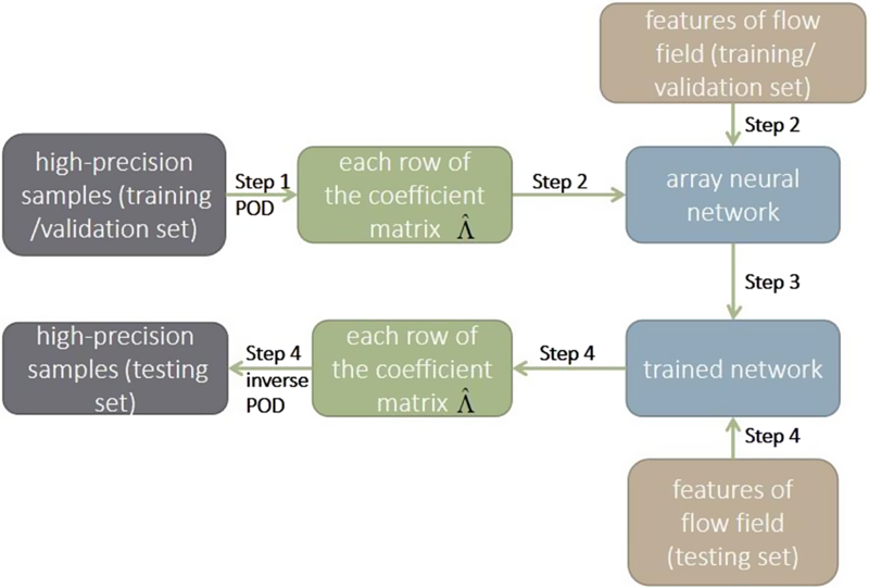
In summary, the basic idea of the array neural network method in this article can be shown as follows:
-
Step 1: We use the POD method to decompose a set of flow fields into a set of basic modals, so that each flow field can be expressed by the basic modals and a weighted sum of coefficients. The basic modals are common to this group of flow fields, while the coefficients are unique to each flow field.
-
Step 2: We use these coefficients for neural network training. Each group of coefficients corresponds to a flow field and also corresponds to the features of this flow field. These features are the Mach number and angle of attack.
-
Step 3: Through such training, we can get a trained network that can predict the modal coefficients at different Mach numbers and angles of attack.
-
Step 4: Through the trained network, we can predict the modal coefficients and the modals, and then we combine them. After that we can reconstruct or predict the flow field through the inverse POD process.
Figure 4 shows the process in detail.
The flow chart of array neural network method.

5.0 RESULTS AND DISCUSSION
5.1 Results
In this section we demonstrate the flow field reconstruction under typical conditions, such as wing flow. Before drawing conclusions, it should be noted that it is necessary to incorporate as much knowledge as possible when we construct array neural networks. Because ANN is only used for the construction of unknown relationships, it should be supplemented by perfect theories or attributes. In order to reduce the number of samples required, the number of neurons of input layer and output layer should be minimised. In addition, due to the theoretical basis of ANN, the solution vectors of the ANN output must be determined by the input parameters. That is to say, the given samples must satisfy the mapping between the input and the output.
All examples in our paper were performed on the Intel CORE i5 7th Gen platform. The running time averages about 0.1 seconds for a training round. Because the training time varies with factors such as the number of neurons, training samples, and so on. The maximum number of training steps set by all the examples is 300,000 times. However, the difference between the samples and the rows of
 $\hat \Lambda $
may result in over-fitting. Thus the number of the stop training step is different. Therefore, not each branch network will reach the maximum number of training step.
In this paper, we choose the flow field data of the NACA0012 airfoil(Reference Shojaeefard, Khorampanahi and Mirzaei26) in the subsonic and wide range of angle of attack to study, which is under the calculation condition of Mach number 0.3, Reynolds number 6.98e6, and the range of angle of attack is −10°~10°, whose interval is 0.1°. Table 1 shows the distribution of samples. All examples are the airfoil flow fields we described above. The dimension of all the original flow field data is 7564, which is same as the size of the grid. The solution vector selected by all the examples is the pressure, and the features of flow field are the Mach number and the angle of attack(Reference Watanabe, Ishimoto and Yamamoto35,Reference Kurganov and Tadmor36) .
Sample distribution

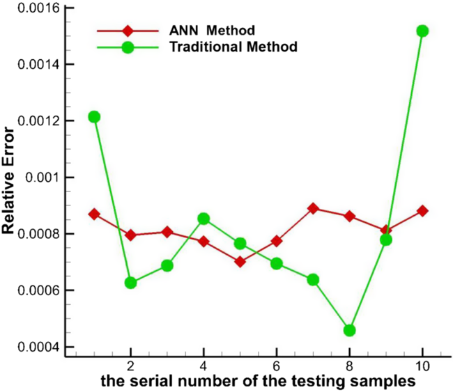
Figure 5 shows the relative error of the array neural network method and the traditional neural network method on the same testing set. The abscissa represents the serial number of the testing samples, and the ordinate represents the relative error between the high-precision samples and the high-dimensional prediction samples. This figure reflects the relative error of each sample between the traditional method and the array neural network method.
As can be seen from this figure, the relative error of the array neural network method in this paper is relatively stable, and it doesn’t change when the angle of attack changes, which shows that our method has good universality for samples with different conditions. The reason why the relative errors of the two methods are not so different is that this figure reflects the relative error of the entire flow field, instead of the relative error at one point of the flow field.
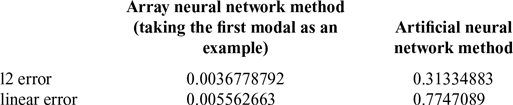
The error in Table 2 is the comparison between modal coefficients of the array neural network and the traditional method. It can be seen that the l2 errors and linearity error of the array neural network method are significantly lower than the artificial neural network method, and the degree of reduction is greater than two orders of magnitude.
The comparison of error between array neural network method and artificial neural network method

The comparison of relative error of flow field reconstruction between the array neural network and the traditional method.

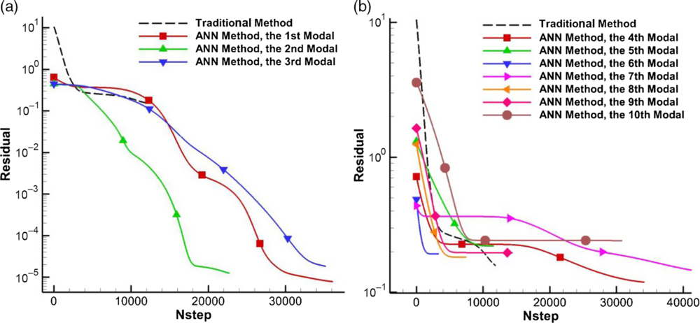
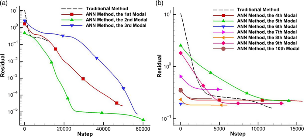
Figures 6 and 7 show the convergence rate and order of the training error and the cost error (the error of the loss function) of the array neural network (the number of modal is ten) and the traditional method. For the convenience of observation, we take the logarithm of base 10. The abscissa represents the number of iterations, and the ordinate represents the training error and the cost error. Figure 6 reflects the trend of training error with the number of iterations. Figure 7 reflects the trend of cost error with the number of iterations.
Training error of the array neural network method and tradition method. (a) modal 1-modal 3 (b) modal 4-modal 10.

Loss function error of array neural network method and tradition method. (a) modal 1-modal 3 (b) modal 4-modal 10.

We have drawn the first three modals and the other modals separately. It can be found that the convergence of the first three modals is very good, and their error can converge to the power of −4 or even −5 of 10, while the traditional method only converges to the power of −1. That is to say, the training error and loss function error of the array neural network are significantly lower than the traditional neural network method. The reason why the phenomenon in the figure appears is that the energy of the first three modals accounts for a large percentage of the overall energy. Actually, each modal represents different information of the flow field. The larger the percentage of the energy the modal has, the more information it represents. The convergence error of the first three modals is very small, which also explains that the array neural network method can reconstruct the flow field well. Therefore, the first few modals of the array neural network have almost determined the convergence rate and convergence order of the error of the whole array neural network, which is one of the reasons why we choose the first few modals instead of all the modals. Another reason will be analysed in detail in the energy analysis subsection of this section.
It can also be seen from Figs 6 and 7 that the error of the traditional method converges in less than 20,000 steps although it is less than that of our method, which means that the traditional method converges quickly. This is because the array neural network method is equivalent to training the information contained in each modal of the flow field, and the neural network has different learning efficiency for each information. However, the traditional method is equivalent to training the information in the flow field together, which is equivalent to mixing the information of all the flow field samples. Since the neural network has different learning efficiency of mixed information and single information, it is reasonable that the traditional method converges faster than the array neural network method in our paper. In addition, in order to prevent overfitting, when the error after iteration 500 steps is larger than the current error, the calculation will automatically stop. This is why the traditional method and the array neural network method have different training convergence iteration steps.
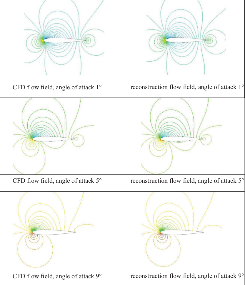
Some of the result of flowfield reconstruction by array neural network method are shown in the Fig. 8. It can be seen that the contour of the reconstructed flow field is smooth, and the flow field structure is correct, which are in agreement with the real flow field (CFD flow field) well.
The comparison between the effects of different angles of attack in CFD flow field and reconstructed flow field, pressure contour, Mach number 0.3.

5.2 The analysis of flow field modal energy
As described in the second section of this paper, the original flow field data matrix
 $A=\left[ {{S_1}\left| \cdots \right|{S_{{M^s}}}} \right] \in {\mathbb{R}^{{M_h} \times {M^s}}}$
has been decomposed into the product of three matrices
 $U,\Sigma $
and
 ${V^T}$
after SVD, where
 $U$
and
 $V$
are orthogonal matrices, and
 $\Sigma $
is an eigenvalue matrix. It can be known from the basic knowledge of advanced algebra that the result of multiplication of the orthogonal matrix and the diagonal matrix is still an orthogonal matrix. Therefore, the matrix
 $\hat \Lambda $
obtained by POD is also an orthogonal matrix. What’s more, the orthogonal vector group must be linearly independent, so each row of the orthogonal matrix
 $\hat \Lambda $
must be linearly independent. According to the linear independence of
 $\hat \Lambda $
and the energy analysis above, the flow field information and energy contained in each row of
 $\hat \Lambda $
are different, which is also not related to each other. Therefore, using a single artificial neural network to predict all the lines of
 $\hat \Lambda $
is not appropriate. This is also the reason why we choose BP neural network algorithm in artificial neural network instead of circulation or convolution neural network algorithm.
 $\Sigma $
is a diagonal matrix, and the eigenvalues on the diagonal are distributed from large to small. The essence of POD is to find a set of optimal standard orthogonal modals
 $\varphi $
of the flow field data matrix
 $A$
, so that the projection of the elements of the flow field data information
 $\left\{ {{S_t}} \right\}|_{t=1}^{{M^s}}$
on this group of modals can be the largest(Reference Yasong, Junqiang and Jun8), namely
 \begin{equation*}\left\{ {\begin{array}{c}{\mathop {\max }\limits_\varphi \dfrac{1}{{{M^s}}}\mathop \sum \limits_{t=1}^{{M^s}} {{\left| {\!\left( {{S_t},{\varphi _i}} \right)} \right|}^2}}\\{\!\left( {\varphi ,\varphi } \right)=1}\end{array}} \right.\end{equation*}
where
 ${(*,*)}$
represents the inner product operation. Theoretically any inner product form can be used. However, in terms of the physical meaning of our paper, the inner product must reflect the physical region solved by the governing equation. In this paper, we use the inner product defined on the square integrable space (L2 space), and
 $\left| * \right|$
is the norm induced by the inner product.
From the perspective of flow field energy, the larger the eigenvalue, the larger the flow field energy. That is to say, the flow field contains more information of data matrix(Reference Jie, Yanhui and Jinsheng7). Thus, we must maximise the generalised “energy” function
 ${\rm{\Upsilon }}\!\left( {podbasic} \right)$
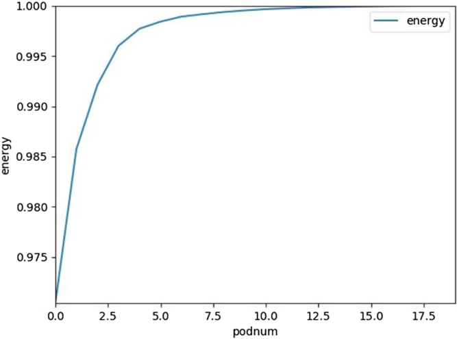
when we ensure that the amount of computation is as small as possible. Figure 9 shows the trend of
 ${\rm{\Upsilon }}$
increasing with the number of modals.
The proportion of energy in modal quantity.

It can be seen from the Fig. 9 that when the number of modals reaches about 10, the energy ratio has been already higher than 99.95%. Therefore, selecting a larger number of modals can’t significantly improve the accuracy of the reconstructed flow field. Instead, it will increase the calculation amount and calculation time; so we choose ten as the number of modals in this paper, which is the second reason for selecting the first few modals.
In summary, this paper adopts array neural network to predict each row of
 $\hat \Lambda $
, the equivalent of which is that each row of
 $\hat \Lambda $
corresponds to a separate neural network. Thus, we can maximise the use of the flow field information contained in each modal, which also meets the conclusion above that there is no correlation between the information of different modals. Thus, we can reconstruct the flow field more comprehensively.
6.0 CONCLUSION
In this paper, we improve the traditional method based on the artificial neural network. A flow field reconstruction method based on array neural network is proposed. Compared to traditional methods, array neural network method has the faster convergence speed and smaller error. What’s more, we have fully considered the linear independence between modals and the fit of the neural network. We choose each row of the matrix Λ as the output of the array neural network method, which significantly reduces the output of the traditional method. This is also one of the most important reasons for the significant increase in accuracy.
In order to test the proposed flow field reconstruction method based on array neural network, a typical testing set is carried out, mainly for airfoil flow field. In general, the proposed method can reconstruct the flow field better and has wide range of application, which can significantly improve the accuracy compared with the traditional method. For the three hidden layers in array neural network, no obvious jumps and huge errors are found in results. In addition, the solution vectors of each sample can be a single component or a combination of multiple field components because the array neural network is nonlinear. We select the single pressure field in this paper, but in fact it is theoretically feasible to output both the pressure field and the velocity field. For the POD method adopted, the calculation time and space loss are significantly reduced with little loss of accuracy, which is obviously superior to the the case of no dimension reduction and all modals are retained.
However, for a typical flow structure, it can be found that when the angles of attack and the Mach numbers of the flow fields are too high, fully considering the entire parameter space is necessary, which needs to increase the number of the input parameters and a large amount of sample data. In this case, the effect of field reconstruction will reduce. This is because the model in this paper is sensitive to parameter changes and the array neural network is data dependent. In a word, the work of this paper is mainly to study the flow field with small angle of attack with good characteristics and the sample set with stable flow field structure. By improving the traditional method, this method has good prediction accuracy for the flow field under such conditions.
Our method does not perform as expected if the flow fields have very different structures. Especially in some areas of the flow field, there will be a phenomenon that the local flow gradient is large, the change is dramatic, and the position is not fixed. That is to say, the effect of field reconstruction will reduce when the flow field has high Mach number and high angle of attack. A flow field with a large angle of attack or a wider speed range will contain more abundant flow field characteristics. Such as shock waves, separation, etc. This makes the energy of the fundamental modes decomposed by the POD method not concentrated, at least the first few modals are not significant. So we may need to improve some aspects, such as increasing sample parameters, improving the depth and complexity of the neural network, considering changing the structure of the array neural network, combining machine learning with other related algorithms and so on. In the future, our work also hopes to deeply study the generalization ability of the method in this paper.
ACKNOWLEDGEMENTS
This study was co-supported by the National Key R&D Program of China (No.2017YFB0202803), the Strategic Priority Research Program (B) of the Chinese Academy of Sciences (No.XDB22020102) and the e-Science Foundation of Chinese Academy of Sciences (No.XXH13506-204).