Implication
Indicator accuracy is of particular concern when indicators are developed for decision-making purpose. One way to improve the accuracy of individual indicators is to combine several ones using logistic regression. Our results show that special attention should be paid to model selection procedure. Models derived without selection were more expensive and slightly less accurate than those derived using a selection procedure. Analysing trade-offs between accuracy and cost of indicators opens promising perspectives as time consuming and expensive indicators are likely to be of low practical utility.
Introduction
Agriculture is pointed to as being one of the major sources of pressure on the environment. High input levels and limited use efficiency of nitrogen, phosphorus, energy and water are responsible for a large amount of pollution. Large-scale studies also indicate that agricultural intensification is one of the main drivers of biodiversity decline in European agro-landscapes (Donald et al., Reference Donald, Green and Heath2001; Donald et al., Reference Donald, Sanderson, Burfield and van Bommel2006). In response to these pressures, a large number of agro-environmental indicators (AEIs) were developed to provide information on the relation between agricultural management and its impact on resource use and the environment (e.g. organisation for economic co-operation and development (OECD, 2003)) and reviews in Van der Werf and Petit (Reference Van der Werf and Petit2002), Halberg et al. (Reference Halberg, van der Werf, Basset-Mens, Dalgaard and de Boer2005), Bockstaller et al. (Reference Bockstaller, Guichard, Makowski, Aveline, Girardin and Plantureux2008)). AEIs can serve several purposes in different application areas: (i) assessing the environmental impact of different management practices or farming systems; (ii) monitoring either changes in the environment or agro-environment policies; and (iii) facilitating communication among different kind of stakeholders around problem definition and acceptable thresholds.
Globally, the scientific community agrees that AEIs should share some common properties, whatever their purpose is. Examining properties considered as important by several authors, Langeveld et al. (Reference Langeveld, Verhagen, Neeteson, Van Keulen, Conijn, Schils and Oenema2007) conclude that effective AEIs should be quantifiable, scientifically sound, refer to relevant issues, acceptable to the target groups involved, easy to interpret and cost effective. To date, very few studies have simultaneously addressed properties of several AEIs. In dairy production systems, Thomassen and de Boer (Reference Thomassen and de Boer2005) compared 13 AEIs derived from input–output accounting of nutrients or product-oriented approaches (ecological footprint and life cycle analysis). Their results indicate that the different sets of indicators differ in terms of relevance, sensitivity over space, reliability and data availability. For nitrogen management, Langeveld et al. (Reference Langeveld, Verhagen, Neeteson, Van Keulen, Conijn, Schils and Oenema2007) showed that nitrogen surplus can be cheaper, more practical in discussion with farmers and more easily translated in day-to-day farmer decision making than ground water nitrate concentration.
Along with these general properties, other works have focused on indicator accuracy, advocating its measurements before selecting any AEIs for practical use (Makowski et al., Reference Makowski, Tichit, Guichard, Van Keulen and Beaudoin2009). Accuracy traduces how well a given AEI separates one state from another (e.g. different level of nitrogen surplus might either represent acceptable or unacceptable levels of pollution). Indicator accuracy is of particular concern when AEIs are developed for decision-making purpose. Accurate AEIs should be able to correctly identify a situation that meets certain criteria as well as to correctly identify a situation that does not meet certain criteria. For such dichotomous situation, the area under the receiver operating characteristics (ROC) curve gives a measure of accuracy (Swets, Reference Swets1988; Murtaugh, Reference Murtaugh1996). It plots the true-positive proportion (TPP) (sensitivity) against the false-positive proportion (1−specificity) for the different possible cut points of an indicator. An area of 1 represents a perfect indicator; an area of 0.5 represents a worthless indicator. Variation in accuracy can be extremely large as reported by Makowski et al. (Reference Makowski, Tichit, Guichard, Van Keulen and Beaudoin2009) for 30 AEIs. One way to improve the accuracy of individual indicators is to combine several ones using logistic regression (Primot et al., Reference Primot, Valantin-Morison and Makowski2006). However, the benefit resulting from this approach may be limited because of (i) uncertainty in input variables, equation and parameter estimation, (ii) the selection of the most appropriate set of indicators (Whittingham et al., Reference Whittingham, Stephens, Bradburry and Freckleton2006), (iii) the acquisition cost of the model input variables.
Aim of this paper was to assess whether accuracy can be increased at a reasonable cost by mixing individual indicators into models. We focused on indicators developed with information collected on management practices. We explore whether these indicators could be considered as ‘proxy’ indicators and could, therefore, represent an alternative to the direct impact measurement on biodiversity. In this study, biodiversity was represented by two grassland bird species with high conservation value, the lapwing Vanellus vanellus and the redshank Tringa totanus. Owing to their high position in trophic networks and their close connection with wet grasslands, these wader species give good information about ecosystem health (Flint, Reference Flint1998). First, we assessed the accuracy of a set of individual indicators, based on management practices, for predicting the presence of these bird species. Second, individual indicators were combined into models using 10 different statistical procedures and the accuracy and cost of implementation was evaluated for each model. The results were used to analyse the interest of combining different types of indicators and the performance of several statistical procedures.
Material and methods
Data
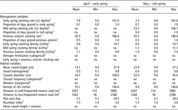
A set of 252 grassland fields located in the Poitevin marsh (France) was monitored for lapwings and redshanks. Surveys were conducted during spring 2004 and 2005 (mid February to July) to determine the presence/absence of both species in each field during their incubation stage (April and May for lapwings and redshanks, respectively). Lapwings were present in 81 fields (21%) and redshanks in 51 fields (12%). Habitat and management indicators measured in each field are presented in Table 1. These indicators described sward cover and field characteristics (10 indicators and one interaction) as well as the management regimes implemented in fields (10 indicators and one interaction). Management indicators were based on fertilisation levels and nine grazing variables (stocking rate, stocking density and proportion of days grazed). These were calculated for three periods (autumn year-1, April i.e. early spring, and May i.e. mid spring). See Durant et al. (Reference Durant, Tichit, Fritz and Kernéïs2008a) for a comprehensive description of the whole data set and observational design.
Means and ranges of management and habitat variables collected in April and May (2004 and 2005) on 252 plots

LU = livestock units (one LU equals the approximated demand of a mature suckling cow: 15 kg DM/day); DM = dry matter; Min = minimum; Max = maximum; na = not applicable (i.e. either categorical variable or time dependent variable not relevant with measurement period).
Data from Poitevin marsh, France (Durant et al., Reference Durant, Tichit, Fritz and Kernéïs2008a).
1Variable calculated following Durant et al. (Reference Durant, Tichit, Fritz and Kernéïs2008a).
2Nitrogen fertilisation level (kg N/ha per year): 0, (1 to 30), (31 to 70).
3Proportion of the field surface covered by tussocks: none, (<5%), (5% to 15%), (16% to 35%), and localised (absent or sparse over most of area but frequent or abundant in remainder).
4Proportion of field surface occupied by water: 0, <5%, (5% to 20%), (21% to 50%), and >50%.
Models combining individual indicators into logistic regression
Management and habitat indicators were combined for predicting the probability of occurrence for two bird species in grassland fields using logistic regression models. Two sets of input variables were distinguished: a set, noted ‘MANAG’, including the variables related to grazing regimes and fertilisation (11 variables), and a set noted ‘ALL’, mixing management variables with those describing habitat quality (11 variables).
When faced with a large number of input variables and the task of selecting a subset of those variables, automated model selection procedures are usually used (Grafen and Hails, Reference Grafen and Hails2004). For each set of input variable and each bird species, 10 different logistic models were thus developed using different automated procedures representing the most commonly used in life sciences. The first one, denoted NS (for no selection), included all input variables (either MANAG or ALL) and its parameters were estimated from the data using the maximum-likelihood method. This method was implemented with the ‘glm’ function of the R-statistical software (http://www.r-project.org/). Four models were developed using four different iterative statistical selection procedures based on the Akaïke’s information criterion (AIC) (Akaike, Reference Akaike1974); forward selection (FW-AIC), backward selection (BW-AIC), stepwise forward selection (SW-FW-AIC) and stepwise backward selection (SW-BW-AIC). The parameters of these four models were estimated by maximum likelihood. Four additional models were developed by implementing forward selection, backward selection, stepwise forward selection and stepwise backward selection with the Bayesian information criterion (BIC) (Schwarz, Reference Schwarz1978) (FW-BIC, BW-BIC, SW-FW-BIC and SW-BW-BIC). Finally, the last logistic model was developed using Bayesian model averaging (BMA) technique described by Viallefont et al. (Reference Viallefont, Raftery and Richardson2001). In some applications, BMA was found to improve the accuracy of model predictions and may lead to more realistic confidence intervals (Raftery and Zheng, Reference Raftery and Zheng2003). Its practical value has recently been studied in an agronomic context (Barbottin et al., Reference Barbottin, Makowski, Le Bail, Jeuffroy, Bouchard and Barrier2008; Prost et al., Reference Prost, Makowski and Jeuffroy2008). BMA method was implemented using the BMA package of the R software (function ‘bic.glm’). The total number of models was equal to 40 (2 bird species × 2 set of input variables×10 statistical methods).
Individual indicators and model performances
The ROC methodology (Swets, Reference Swets1988; Murtaugh, Reference Murtaugh1996) was used to evaluate the ability of each indicator or model to discriminate between fields with birds’ presence and fields with birds’ absence. The procedure proposed by Hughes et al. (Reference Hughes, McRoberts and Burnett1999), Makowski et al. (Reference Makowski, Taverne, Bolomier and Ducarne2005) and Primot et al. (Reference Primot, Valantin-Morison and Makowski2006) was applied to our data set. Hereafter, the procedure is detailed for models; readers can refer to Makowski et al. (Reference Makowski, Tichit, Guichard, Van Keulen and Beaudoin2009) for its application on individual indicators.
For each bird species, the set of grassland fields was divided into two subgroups, depending on whether the bird was present, y = 1, or absent, y = 0. The output variable of each model (i.e. the probability of bird presence) was computed for each field of each subgroup. Model outputs were compared to a threshold (PT) to estimate the true positive proportion (TPP) and the true negative proportion (TNP). TPP and TNP correspond to the estimated values of the sensitivity and specificity of the model for a given threshold PT. This procedure was repeated for all possible thresholds PT and the results were used to compute the area under the ROC curve (AUC) with the ROCR package (Sing et al., Reference Sing, Sander, Beerenwinkel and Lengauer2005). The AUC of a model is equal to the probability of correctly ranking two fields with and without birds on the basis of model predictions. AUC is expected to be equal to 0.5 for a non-informative model, and 1 for a perfect model. In order to limit the risk of underestimation of model errors, sensitivity specificity and AUC values were estimated by cross validation (Primot et al., Reference Primot, Valantin-Morison and Makowski2006; Wallach, Reference Wallach2006).
Cost of habitat and management variables
The cost associated with each individual variable was computed according to the time spent for data collection either on field or farms, the number of surveys or measurements needed and the method of measurement. Other costs such as those related to data base creation, software and computing equipment were not taken into account because they are difficult to relate to a specific study with high reliability. Five categories of variables characterized by different costs were defined (Table 2). Management variables were derived from one or several interviews conducted by a single technical assistant on 67 farms. Field management data, such as fertilization levels or stocking density were collected during the first interview. More complex management variables such as stocking rates at different periods required repeated phone calls throughout the year. The cost of management variables was calculated as the sum of the personal and phone costs needed to collect the required information. Personal costs corresponded to the product of the number of days spent and the daily personal cost for a technical assistant (184 €/day; data from INRA administration 2007). Phone costs were calculated as the product of time spent and phone call rate (average phone rate of 0.12 €/min ranging from 0.016 € for standard to 0.2 € for cellular phone).
Cost of the different input variables used in the logistic regression for both bird species

Five cost categories were distinguished on the basis of variable sets (management, habitat) and the measurement methods. Data from INRA Saint Laurent de la Prée, France.
Habitat variable were collected on the 252 grassland fields belonging to the 67 farms by eight people (four two-person teams made of one technical assistant and one trainee) during 3 weeks in spring. Some of the variables required repeated measurement in fields and were time consuming (e.g. mean sward height and heterogeneity), whereas others were visually estimated in each field (e.g. water surface, tussock frequency, density of rills) and were thus less costly. Finally a few habitat variables were computed using Geographic Information System (GIS) (e.g. distance to nearest road, size). The cost of habitat variables was calculated as the sum of the personal and operational costs. Personal costs were computed as described for management variables on the basis of 214 €/day for one two-person team (data from INRA administration 2007). Operational costs (i.e. daily travelling cost for eight people to the study area during 3 weeks) were calculated on the basis of kilometric cost in vehicle (0.29 €/km; data from INRA 2007).
Habitat and management variables had different costs because they did not require the same amount of time for data collection. Most of the habitat variables were more expensive because they were time consuming due to the size of the study area (c. 1000 ha) and the repeated measurements carried out within each field.
Results
AUC values obtained for individual indicators
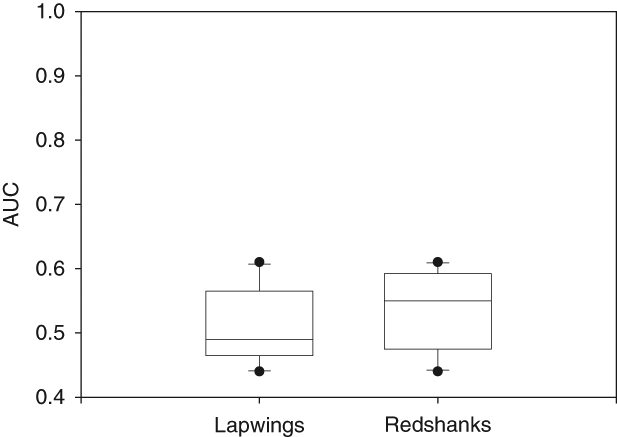
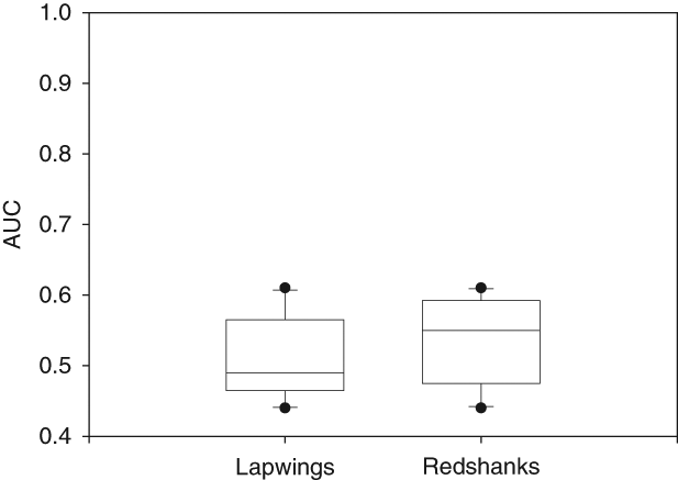
The variation of the AUC values for both bird species computed for management indicators ranged from 0.44 to 0.61. Some of these indicators were thus useless, whereas others were quite informative. Among all indicators, 50% had an AUC lower than or equal to 0.50 and thus were not better than a random decision. For example, the AUC of all indicators based on stocking density (at any period) ranged between 0.44 and 0.49. Other indicators performed better, notably those based on cumulated stocking rates in early spring that reached higher AUC values (0.53 to 0.61). The range in variation of the AUC values was similar for both bird species (Figure 1), and 80% of the indicators performed equally (either good or bad). Two indicators only led to contrasting results between both bird species. The proportion of days grazed in previous autumn was non-informative in lapwings (AUC = 0.47), whereas in redshanks its AUC was higher than the random decision threshold (0.59). Similarly, the cumulated stocking rate in mid spring was a poor indicator in lapwings (AUC = 0.49), whereas it was the best one in redshanks (AUC = 0.61).
Values of the area under the curve (AUC) of management indicators for each bird species. Box plot: minimum, first quartile, median, third quartile, maximum. Analysis based on management variables (1 to 10) from Table 1 (Makowski et al., Reference Makowski, Tichit, Guichard, Van Keulen and Beaudoin2009).
AUC values obtained with models combining individual indicators
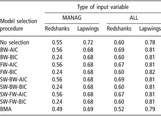
AUC values estimated with cross-validation for the 40 logistic models are shown in Table 3 for both bird species. AUC values ranged from 0.68 to 0.82 for lapwings and from 0.24 to 0.69 for redshanks. For both species, AUC values obtained with ‘ALL’ models were always higher than that obtained with ‘MANAG’ models. In redshanks, 50% of the ‘MANAG’ models had extremely low AUC values (<0.5) indicating that these models were not better than a random decision. In lapwings, AUC values were always higher than 0.5 for all types of input variables (MANAG or ALL). In redshanks, the models with the highest AUC were obtained with AIC (either BW-AIC or SW-BW-AIC). In lapwings, the best model was FW-BIC, but all the stepwise procedures based on AIC and BIC led to very similar AUC values.
Area under the curve values estimated by cross-validation for 20 logistic models (10 model selection procedures and 2 types of input variables) for redshanks and lapwings

BW = backward selection; AIC = Akaïke’s information criterion; BIC = Bayesian information criterion; FW = forward selection; SW-BW = stepwise backward selection; SW-FW = stepwise forward selection; BMA = Bayesian model averaging.
Model performance was not always higher than that of individual indicators. In lapwings, ‘MANAG’ models always had higher accuracy than any single indicators. However, in redshanks combining management variable into models slightly decreased accuracy when compared with the best performing individual indicator. For this species, only the ‘ALL’ models based on AIC led to an increased accuracy in comparison with the best individual indicator.
Important indicators for birds
We do not give parameter values in this study, as our objective was to assess the performance of individual indicators or models in predicting the presence/absence of birds, and not to estimate the effects of explanatory variables. These effects are only briefly presented below. High levels of fertilisation had a negative effect on field selection by both species, in particular when the amount of applied nitrogen was higher than 30 kg /ha per year. Grazing intensity or the proportion of days grazed in early spring favoured the presence of both species. Increasing mean sward height and the absence of field wetness had a negative effect on the probability of presence of both species. The interaction between mean sward height and wetness was positive, suggesting that birds could occupy fields with higher mean sward height than expected when wetness was high (i.e. more than 21% of the field area). Large field size also had a positive effect on the probability of presence of both species. More detailed results about the effects of these variables are presented in Durant et al. (Reference Durant, Tichit, Fritz and Kernéïs2008a).
Model cost v. model accuracy
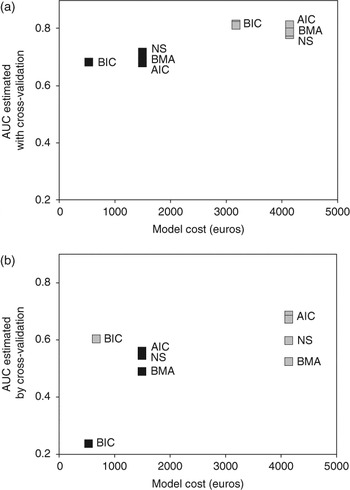
The AUC value of each model was plotted against its cost (Figure 2). In lapwings, models including management variables were the cheapest (531 to 1493 €) and those combining all input variables were the most expensive (3174 to 4136 €) (Figure 2a). Among the ‘MANAG’ models, the cheapest ones were those based on BIC (531 €) and the more expensive ones were those derived without selection (full model and BMA) or based on AIC. The full model only led to a slight increase in accuracy. ‘MANAG’ models obtained with BMA or AIC were nearly three times more expensive, but with the same level of accuracy than those obtained with BIC. Among the ‘ALL’ models, the most expensive ones were the full models, those derived by BMA, and the models selected using AIC, whereas those selected using BIC were cheaper. The use of AIC instead of BIC led to models with five additional variables and thus to a higher cost. Although more expensive, the full model and that derived by BMA were slightly less accurate than the less costly models derived using selection procedures based on BIC.
Cost v. accuracy of each model for lapwings (a) and redshanks (b). Models based on management variables ( ) or combining habitat and management variables (
 ). Models based on management variables (1 to 11) and all variables (1 to 22) from Table 1. Data from Poitevin marsh, France.

Figure 2b shows that the most expensive models for redshanks were ‘ALL’ models obtained without selection (NS or BMA) and those derived using selection procedures based on AIC (4136 €). The ‘ALL’ models based on BIC were the cheapest ones (669 €) as they included a lower number of explanatory variables. Several ‘MANAG’ models obtained with BIC had an AUC lower than 0.5 and were thus useless. For a given cost, the models derived from a selection procedure based on AIC were more accurate than full models and models obtained by BMA. Compared with individual indicators, best ‘MANAG’ models (based on AIC) did not provide any advantage, as their accuracy was slightly lower (AUC = 0.56) than that of the best performing individual indicator (Mid-spring stocking rate, AUC = 0.61) and obviously they were more costly.
Discussion
Our results showed that the levels of accuracy of different AEIs varied strongly. The performance of some individual AEIs was very poor, whereas others were quite informative. Measuring indicator accuracy can thus be considered as a useful preliminary step before selecting the best one.
Low accuracy of AEIs based on management information was also reported for several environmental issues (Makowski et al., Reference Makowski, Tichit, Guichard, Van Keulen and Beaudoin2009). These authors showed that AEIs on the basis of information about habitat quality performed better than those on the basis of management practices. A possible explanation is that habitat quality is often the last step in the chain of relations between field management and reference environmental variables (e.g. birds). Each step in this chain adds extra uncertainty and variability (ibid). Poor performances of AEIs based on management information are problematic, especially when scientists advocate that AEIs should be based on management practices (Van der Werf and Petit, Reference Van der Werf and Petit2002) or when considering their central role in the definition of environmental prescriptions (Henkens and Van Keulen, Reference Henkens and Van Keulen2001). Management variables are proxies for complex processes, which may (at least partly) explain why they are poor indicators. For instance, indicators based on stocking density performed poorly for both bird species at any time period. They relate animal number to field area and assume homogeneous field use by livestock. However, several studies have reported that field use is not homogeneous and factors such as distance to drinking water, slope, wetness and field characteristics (e.g. size, management) may influence the spatial and temporal variability of grazing pressure (Dumont et al., Reference Dumont, Meuret, Boissy and Petit2001). This variability in grazing pressure can generate differences in sward states, which play an important role in field selection by birds.
We showed that in some situation it may be better to use a combination of all indicators than a single indicator. However, our results also showed high variability in the accuracy of the different models. A few models were not better than a random decision rule for presence/absence (e.g. in redshanks). Others were more accurate, especially for lapwings where several models had AUC values higher than 0.8. Whatever the type of input variable, lapwing models always had higher AUC than redshank models. Both species differed in their prevalence (higher in lapwings than in redshanks), however this difference cannot explain variation in model performance (Manel et al., Reference Manel, Williams and Ormerod2001; McPherson et al., Reference McPherson, Jetz and Rogers2004). As underlined by these authors, AUC is largely unaffected by species prevalence.
Species ecological requirements may explain some of the observed differences for at least three reasons. First, lapwings are more favoured than redshanks by the cumulated effects of grazing (Tichit et al., Reference Tichit, Renault and Potter2005; Durant et al., Reference Durant, Tichit, Fritz and Kernéïs2008a); second, they respond to grazing in interaction with the quality of their environment, notably field wetness (Milsom et al., Reference Milsom, Langton, Parkin, Peel, Bishop, Hart and Moore2000; Durant et al., Reference Durant, Tichit, Fritz and Kernéïs2008a) and finally they have stricter habitat requirements than redshanks (Durant et al., Reference Durant, Tichit, Kerneis and Fritz2008b). It is thus easier to predict their presence/absence from variables based either on management or management and habitat.
Models combining both types of variables were the most accurate. Combining both types of variables led to an increase in accuracy, notably for species with larger habitat preferences such as the redshank. AUC values for these models were higher than the values reported for the individual variables. Our results thus showed the interest of combining different types of variables for predicting the presence/absence of bird species.
The best models were those developed using a selection procedure based either on AIC or BIC depending on the bird species. These models performed better than the full models and the models derived by BMA. Selection procedures were able to reduce the number of explanatory variables, to reduce the costs and to increase model performance. Selection algorithm (forward, backward and stepwise) did not influence model accuracy. However, the selection criterion (AIC, BIC) influenced the number of variables included in models and their AUC. Models selected with BIC had a lower variable number than the models selected with AIC. This is consistent with earlier results showing that BIC tended to be more conservative (Prost et al., Reference Prost, Makowski and Jeuffroy2008). Although the AUC obtained with AIC and BIC were quite similar for lapwings, this was not the case for redshanks where BIC led to smaller AUC values. Here again, this difference may be because of the different requirements of the two bird species. Lapwings being highly sensitive to small variation in habitat quality, the use of either BIC or AIC led to the same level of AUC for this species. With larger ecological requirements, redshanks’ models based on BIC were more parsimonious but less accurate.
It is impossible to make a rational selection among indicators without any information on their accuracy, our results also showed that cost is another essential property to take into account. Correlation between model accuracy and cost of implementation was positive; however the most costly models were not always the most accurate. Models derived without any selection and by BMA were the most costly because they included all the candidate explanatory variables. These models were not the most accurate as they had too many parameters compared with models selected using either AIC or BIC. The cheapest models were those derived using BIC because this criterion led to very simple models. When BIC-based selection procedures were applied to models based on both habitat and management variables, resulting models were quite accurate and corresponded to a very good compromise between cost and accuracy. On the other hand, the use of BIC with a restricted number of candidate explanatory variables led to inaccurate models, especially for redshanks. In such cases, the resulting models were too parsimonious.
Conclusion
Our results show that the accuracy of AEIs, either complex or simple ones, should be systematically measured using observational or experimental data. Mixing management indicators into models can improve accuracy, but it is necessary to pay special attention to model selection strategies. Models developed without any selection procedure are more costly and less accurate. Indicators cost is another important issue as time consuming and expensive AEIs are likely to be of low practical utility.
Acknowledgements
The work of David Makowski was funded by the Agence National de la Recherche (ANR) call JCJC (Picsel project). Data were kindly provided by INRA Saint Laurent de la Prée. We thank D. Durant, P. Faure, P. Grene, J. M. Hillaireau, E. Kernéïs, N. Lemaire and Olivier Schmit, who participated to the fieldwork. We also thank two referees for their constructive feedback.