Nomenclature
-
 $h \,$
(km)
-
altitude
-
$V \,$
(m/s)
-
Earth-relative velocity
-
$\theta \,$
(rad)
-
longitude
-
$\phi \,$
(rad)
-
latitude
-
$\psi \,$
(rad)
-
heading angle
-
$\gamma \,$
(rad)
-
flight path angle
-
$\alpha \,$
(rad)
-
angle-of-attack
-
$\sigma \,$
(rad)
-
bank angle
-
${\psi }_{LOS}\,$
(rad)
-
line-of-sight angle
-
${\Delta }\psi \,$
(rad)
-
line-of-sight angle error
-
$g \,$
(m/s
$^{2}$
)
-
gravitational acceleration
-
$D \,$
(N)
-
aerodynamic drag force
-
$L \,$
(N)
-
aerodynamic lift force
-
$\rho \,$
(kg/m
$^{3}$
)
-
atmospheric density
-
$m \,$
(kg)
-
mass of the vehicle
-
${S}_{m} \,$
(m
$^{2}$
)
-
reference area
-
$Q \,$
(kW/m
$^{2}$
)
-
heating rate at a specified point
-
$n \,$
(m/s
$^{2}$
)
-
aerodynamic load
-
$q \,$
(Pa)
-
dynamic pressure
-
${R}_{e} \,$
(m)
-
Earth radius
-
$r \,$
(m)
-
radial distance of the vehicle to the Earth centre
-
${\omega }_{e} \,$
(rad/s)
-
Earth angular velocity


1.0 Introduction
Hypersonic glide vehicles (HGVs) have emerged as critical platforms for next-generation aerospace operations, leveraging their wide-speed-regime manoeuvrability and large-scale cross-domain capabilities in near space. Their unique aerothermodynamic adaptation mechanisms and morphing control characteristics have attracted significant research attention [Reference Shen, Yu, Dong, Hua and Ren1–Reference Yu, Li and Zhang3]. However, with the maturation of space-based infrared detection constellations and multi-layered ground-based kinetic interception defenses, these vehicles now face dual suppression from all-time-domain surveillance threats and cross-medium coordinated strikes. Concurrently, the proliferation of avoidance zones comprising geopolitically sensitive areas and multilateral policy buffer regions necessitates real-time autonomous evasion strategy generation. Developing intelligent penetration guidance architectures with environmental responsiveness thus becomes essential to overcome mission constraints imposed by complex flight environments [Reference Wu, Wang, Liu, Li and Yu4].
Under rigidly anchored terminal point constraints, reentry guidance schemes for HGVs bifurcate into two categories: nominal trajectory guidance and predictor-corrector guidance. The core principle of nominal trajectory guidance involves offline design of flight trajectories satisfying all constraints, with mission execution achieved through online trajectory tracking. This approach offloads computational burden, reducing demands on onboard computing resources, yet lacks responsiveness to environmental uncertainties and fails to accommodate state perturbations or deviations [Reference Wang, Guo, Tang, Qi and Wang5, Reference Zhang, Chen, Liu, Tang and Bao6]. In contrast, predictor-corrector guidance dynamically adjusts flight strategies based on real-time vehicle states and environmental dynamics, thereby achieving both guidance precision and robustness [Reference Lu7–Reference Xue and Lu10]. Against the backdrop of rapid advancements in onboard hardware, the predictor-corrector framework emerges as the superior paradigm for developing intelligent penetration algorithms.
The fundamental framework of predictor-corrector comprises longitudinal and lateral guidance links. The lateral guidance link directly regulates the heading by controlling line-of-sight angle error, with its core concept being to determine the expected reference heading and adjust the reversal logic of the bank angle accordingly. This approach is widely adopted by researchers in constructing penetration guidance strategies for reentry vehicles under no-fly-zone (NFZ) constraints. Mature methodologies for determining expected reference headings in NFZ environments fall into two categories. The first establishes reference headings via geometric relationships between NFZs and the vehicle. Serving as reference points for adjusting bank angle reversal logic, NFZs and key waypoints guide the vehicle through lateral guidance cycles [Reference Wang, Zhang and Tang11]. Liang et al. [Reference Liang, Liu, Li and Ren12] achieved NFZ avoidance by designing expected waypoints, whose vectors incorporate the position and directional constraints of the trajectory. While this method reduces the computational complexity of determining the reference heading, it necessitates precise manoeuvres within a narrower solution space and requires designing rational waypoint strategies. The second category calculates reference headings in real-time using the concept of field. Common approaches include the interfered fluid dynamic system (IFDS) and artificial potential field (APF) methods. For the IFDS-based obstacle avoidance principle, disturbance functions are introduced into an ideal flow field to generate collision-free navigation streamlines [Reference Tamanakijprasart, Mondal and Tsourdos13, Reference Yao, Wang and Su14]. Celestini et al. [Reference Celestini, Primatesta and Capello15] proposed a 3D trajectory planning strategy combining IFDS with Bézier curves under multiple obstacle constraints. Wu et al. [Reference Wu, Wang, Zhang and Yu16] integrated the concept of receding horizon control with IFDS to establish a 3D path planning framework for non-convex obstacle environments. The core principle of APF-based obstacle avoidance involves driving a moving object toward the target while avoiding obstacles through virtual potential field forces, essentially constructing a superimposed field of target-attractive and obstacle-repulsive potentials [Reference Warren17–Reference Duhé, Victor and Melchior19]. A lateral guidance algorithm combining APF with velocity azimuth error corridors was designed to reduce heading errors and achieve NFZ avoidance while addressing terminal and path constraints [Reference Zhang, Liu and Wang20]. Hu et al. [Reference Hu, Gao, Li, Jing and Chen21] developed an improved APF method to formulate NFZ judgement criteria and determine reference headings, along with an adaptively updated real-time heading corridor for distributed NFZ constraints. Due to HGVs’ long-range and wide-velocity envelope manoeuvring patterns, migrating IFDS-based solutions to HGV penetration strategies carries risks such as disturbance attenuation, global information dependency and computational complexity divergence. In contrast, APF-based approaches are more compatible due to higher computational efficiency, lower dependency on global information and stable behavioural patterns.
However, although the aforementioned schemes demonstrate satisfactory avoidance performance in preset scenarios, it must be acknowledged that critical algorithmic parameters such as potential field functions and weighting coefficients exhibit strong environmental sensitivity. Yet these key parameter sets typically rely on simplified manual adjustment rules with online loading, lacking timely feedback and targeted adjustments based on environmental state awareness throughout mission execution. Therefore, developing efficient sensitive parameter set tuning strategies to enhance the adaptability of vehicle avoidance algorithms is imperative. Scholars have achieved certain progress by developing heuristic algorithm-based optimisers: Wu et al. [Reference Wu, Dai, Jiang and Karimi22] introduced a method using a deterministic annealing strategy to improve potential field functions through temperature parameter incorporation. A dynamic enhanced firework algorithm was applied to resolve local minima issues in traditional artificial potential field functions, with experimental verification confirming trajectory safety and smoothness enhancements [Reference Li, Liu, Yang, Wang, Qie and Xiang23]. Nevertheless, heuristic algorithms remain fundamentally stochastic function optimisers dependent on static fitness functions to evaluate solution quality and incapable of perceiving state transitions in dynamic environments. This inevitably causes frequent failures in non-stationary scenarios. Crucially, the high dynamic motion pattern induces intense and frequent state changes in HGVs. Moreover, HGVs impose extremely demanding computational efficiency requirements on optimisers. Given the generally high computational complexity of heuristic algorithms, they represent a suboptimal choice.
As artificial intelligence technology advances at a fast pace, online real-time optimisation frameworks built on deep reinforcement learning (DRL) have stood out as more effective options for adjusting sensitive parameters. These frameworks find wide use in adaptive optimisation, control systems and other relevant fields [Reference Yin, Fang and Wang24, Reference Tong, Song and Li25]. Compared to heuristic-based algorithms, DRL functions as an environment-interactive policy optimiser that explicitly models temporal causality between states and actions through Markov decision processes (MDPs), thereby possessing online environmental response capabilities. Additionally, DRL’s pre-trained policy networks can rapidly adapt to similar tasks via fine-tuning, significantly reducing cross-scenario deployment costs. Luo et al. [Reference Luo, Wang and Pan26] introduced a virtual potential field detection zone to enhance the artificial potential field method, integrated with a long short-term memory (LSTM) network-based reinforcement learning agent for online adjustment of detection zone radius to achieve obstacle avoidance for unmanned vehicles. However, when designing online efficient avoidance strategies for HGVs using artificial potential field methods, targeted improvements to conventional approaches must account for both vehicle-specific characteristics and flight environment properties, while ensuring the online self-adaptiveness of modified models.
Inspired by the above literature review, this paper proposes a learning-based APF penetration guidance algorithm for HGVs under multi NFZ constraints, with primary contributions summarised as follows:
-
(1) Comprehensive consideration of HGV-specific characteristics and flight environment properties establishes an APF benchmark model and its sensitive parameter sets suitable for long-range flight under multiple NFZ constraints. This benchmark model facilitates reference heading design in preset flight scenarios while mitigating conflicts among obstacle avoidance, trajectory smoothing and target reachability.
-
(2) To eliminate dependencies on preset parameters and scenarios in the APF benchmark model while enhancing environmental adaptability and robustness, a DRL agent based on the twin-delayed deep deterministic policy gradient (TD3) framework and transformer backbone architecture is designed for online tuning of the benchmark model’s sensitive parameter sets. This agent dynamically adjusts each parameter element by capturing contextual relationships within temporal observations to further optimise avoidance effectiveness.
-
(3) Building upon reference headings jointly generated by the DRL-based sensitive parameter optimiser and the APF benchmark model, lateral guidance cycles determine bank angle reversal logic to achieve vehicle heading correction. When integrated with longitudinally designed numerical predictor-corrector strategies, a learning-based artificial potential field guidance framework for HGV penetration is proposed.
The subsequent content of this paper is organised as follows. Section 2 provides mathematical problem formulation for HGV penetration guidance, encompassing vehicle dynamics and enforced constraints. Section 3 establishes the learning-based artificial potential field penetration guidance framework, including the APF benchmark model with its sensitive parameter sets and the learning-enabled penetration guidance architecture. Section 4 validates strategy efficiency through numerical simulations and provides corresponding analyses. Section 5 concludes the paper.
2.0 Problem formulation
This section systematically describes the flight dynamics of HGV reentry penetration and multiple enforced constraints.
2.1 Reentry dynamics
Given the extensive range and wide velocity envelope of HGVs during reentry glide, the Earth is modeled as a rotating sphere. On this basis, the complete equations of motion are established, in which the first three dynamic equations govern the evolution of the velocity vector (including its magnitude and flow angles), while the remaining three kinematic equations map the vehicle’s position within the spherical coordinate system [Reference Tong, Song, Xu and Yu2, Reference Yu, Dong, Li, Ren and Lv27, Reference Xu, Cai, Mu and Li28]
 \begin{align}\left\{\begin{array}{ll}\dfrac{\mathrm{d}V}{\mathrm{d}t}&= {} -\dfrac{D}{m}-g \sin \gamma +{\omega }_{e}^{2}r \cos \phi (\! \sin \gamma \cos \phi \\[8pt] {} &\quad- \cos \gamma \sin\phi \cos \psi )\\[6pt] \dfrac{\mathrm{d}\gamma }{\mathrm{d}t}&= {} \dfrac{1}{V}\bigg[\dfrac{L \cos \sigma }{m}-g \cos \gamma +\dfrac{{V}^{2} \cos \gamma }{r}+2{\omega }_{e}V \cos \phi \sin \psi \\[8pt] {} &\quad+{\omega }_{e}^{2}r \cos \phi (\! \cos \gamma \cos \phi + \sin \gamma \sin\phi \cos \psi )\bigg]\\[8pt] \dfrac{\mathrm{d}\psi }{\mathrm{d}t}&= {} \dfrac{1}{V}\left[\dfrac{L \sin \sigma }{m \cos \gamma }+\dfrac{{V}^{2} \cos \gamma \sin \psi \tan \phi }{r}\right.\\[10pt] {} &\quad-2{\omega }_{e}V(\! \tan \gamma \cos \phi \cos \psi - \sin\phi )\\[6pt] {} &\quad\left.+\dfrac{{\omega }_{e}^{2}r}{ \cos \gamma } \sin\phi \cos \phi \sin \psi \right]\\[9pt] \dfrac{\mathrm{d}r}{\mathrm{d}t}&= {} V \sin \gamma \\[8pt] \dfrac{\mathrm{d}\theta }{\mathrm{d}t}&= {} \dfrac{V \cos \gamma \sin \psi }{r \cos \phi }\\[8pt] \dfrac{\mathrm{d}\phi }{\mathrm{d}t}&= {} \dfrac{V \cos \gamma \cos \psi }{r}\end{array}\right.\end{align}
 \begin{align}\left\{\begin{array}{l}L=\frac{1}{2}\rho {V}^{2}{C}_{L}{S}_{m}\\[4pt] D=\frac{1}{2}\rho {V}^{2}{C}_{D}{S}_{m}\end{array}\right.\end{align}
where
 $\rho ={\rho }_{0}\exp\!({-}h/{h}_{s})$
denotes the atmospheric density at flight altitude,
 ${\rho }_{0}$
is the sea-level atmospheric density and
 ${h}_{s}$
denotes the standard reference altitude.
Considering that aerodynamic characteristics are highly vehicle-dependent, the Common Aero Vehicle (CAV-H) is adopted as the benchmark vehicle in this paper. Consequently, the corresponding aerodynamic coefficients
 ${C}_{L}$
and
 ${C}_{D}$
are formulated as nonlinear functions of the angle-of-attack
 $\alpha $
and velocity
 $V$
[Reference Xu, Cai, Mu and Li28], expressed as:
 \begin{align}\left\{\begin{array}{l}{C}_{L}=-0.2355+2.9451\alpha +0.2949\,\exp\!({-}0.0003943V)\\[3pt] {C}_{D}=0.0234+2.3795{\alpha }^{2}+0.3983\,\exp\!(0.0010794V)\end{array}\right.\end{align}
2.2 Multiple constraints
To accomplish long-range reentry glide penetration missions, vehicles must satisfy constraint sets including trajectory safety constraints, target reachability constraints, bounded control constraints and penetration constraints.
(1) Trajectory safety constraints
HGVs endure extreme aerothermodynamic environments during reentry glide, necessitating strict control of critical parameters including heating rate
 $\,\dot{\!Q}$
, g-load overload
 $n$
and dynamic pressure
 $q$
to ensure trajectory safety, mathematically modeled as [Reference Lu7]:
 \begin{align}\left\{\begin{array}{l}\dot{Q}={K}_{Q}{\rho }^{0.5}{V}^{3.15}\le {\dot{Q}}_{ \max }\\[4pt] n=\sqrt{{D}^{2}+{L}^{2}}/\mathrm{m}\mathrm{g}\le {n}_{ \max }\\[4pt] q=\frac{1}{2}\rho {V}^{2}\le {q}_{ \max }\end{array}\right.\end{align}
where
 ${K}_{Q}=7.9686\times 1{0}^{-5}$
is a constant.
Additionally, the quasi-equilibrium glide condition (QEGC) [Reference Xue and Lu10, Reference Guo, Li, Zhang, Wang and Cai29] is incorporated into trajectory safety constraints as a soft constraint to reduce or prevent trajectory oscillation and bouncing during glide, expressed as:
 \begin{align}\frac{L \cos {\sigma }_{EQ}}{m}-g \cos \gamma +\frac{{V}^{2} \cos \gamma }{r}\ge 0\end{align}
where
 ${\sigma }_{EQ}$
represents
 $\sigma $
that complies with QEGC.
By employing QEGC, the inequality constraints in Equation (4) can be transformed into bounded constraints on the magnitude of
 $\sigma $
. Within these bounds, the constraints in Equation (4) can be considered satisfied.
(2) Target reachability constraints
To precisely quantify terminal guidance precision, the final constraints for reentry flight are mathematically expressed as [Reference Wu, Wang, Liu, Li and Yu4]:
 \begin{align}\left\{\begin{array}{l} {\Delta }h=\left|{h}_{t}-{h}_{f}\right|\le {\delta }_{h} {} \\[3pt] {\Delta }V=\left|{V}_{t}-{V}_{f}\right|\le {\delta }_{V} {} \\[3pt] {\Delta }{L}_{r}=\left|{{L}_{r}}_{,t}-{{L}_{r}}_{,f}\right|\le {\delta }_{{L}_{r}} {} \end{array}\right. \\[-15pt] \nonumber \end{align}
where
 ${h}_{t}$
,
 ${V}_{t}$
and
 ${{L}_{r}}_{,t}$
denote altitude, velocity and remaining range upon mission termination, respectively, while
 ${h}_{f}$
,
 ${V}_{f}$
,
 ${{L}_{r}}_{,f}$
,
 ${\delta }_{h}$
,
 ${\delta }_{V}$
,
 ${\delta }_{{L}_{r}}$
represent corresponding desired terminal states and their tolerance thresholds.
The mathematical expression for the remaining range (
 ${L}_{r}$
) to the target is given by:
 \begin{align}{L}_{r}={R}_{e}\mathrm{arccos} [\! \sin\phi \sin{\phi }_{f}+ \cos \phi \cos {\phi }_{f} \cos ({\theta }_{f}-\theta )]\end{align}
where
 $({\theta }_{f},{\phi }_{f})$
denotes the longitude and latitude coordinates of the target point.
(3) Bounded control constraints
Key control variables for reentry guidance include
 $\alpha $
and
 $\sigma $
, both subject to bounded limitations mathematically expressed as:
 \begin{align}\begin{cases}{\alpha }_{ \min }\le \alpha \le {\alpha }_{ \max }\\[3pt] 0\le \left|\sigma \right|\le {\sigma }_{ \max }\end{cases}\end{align}
where
 ${\alpha }_{ \min }$
,
 ${\alpha }_{ \max }$
, and
 ${\sigma }_{ \max }$
denote the boundary values.
(4) Penetration constraints
Penetration constraints mandate strict avoidance of prohibited airspace during reentry flight, including threat zones and geopolitically sensitive regions. These restricted areas are uniformly treated as NFZs and modeled using standard convex polyhedron modeling as follows [Reference Wu, Wang, Liu, Li and Yu4, Reference Tong, Song, Li and Xu8, Reference Wu, Wang, Zhang and Yu16]:
 \begin{align}\left\{\begin{array}{ll}{{\Gamma }}_{k}\left(P\right)&= {} {\left[(\theta -{\theta }_{k})/{a}_{k}\right]}^{2{p}_{k}}+{\left[(\phi -{\phi }_{k})/{b}_{k}\right]}^{2{q}_{k}}+{\left[(\bar{h}-{\bar{h}}_{k})/{c}_{k}\right]}^{2{r}_{k}}\\[3pt] P&= {} \left[\theta ,\phi ,\bar{h}\right]^{T}\end{array}\right.\end{align}
where
 $k=\mathrm{1,2},3, \ldots ,K$
denotes the NFZ index,
 $\bar{h}=(h+{R}_{e})/{R}_{e}$
is the normalised vehicle altitude, and
 ${[{\theta }_{k},{\phi }_{k},{\bar{h}}_{k}]}{}^{T}$
is the centroid coordinates of threat elements. Parameters
 ${a}_{k}$
,
 ${b}_{k}$
,
 ${c}_{k}$
and
 ${p}_{k}$
,
 ${q}_{k}$
,
 ${r}_{k}$
represent radius and shape coefficients of this standard convex polyhedron model.
Equation (9) constitutes a continuously differentiable function monotonically increasing with the distance between adversarial agents.
 ${{\Gamma }}_{k}\left(P\right)\le 1$
indicates the envelope intersection between the penetration vehicle and threat elements, thus the interceptor constraint during adversarial engagement can be defined as:
 \begin{align}{{\Gamma }}_{k}\left(P\right)\gt 1\end{align}
Considering NFZs as cylinders of infinite height, the parameters in Equation (9) are configured as follows:
 ${a}_{k}={b}_{k}={R}_{N,k}$
,
 ${p}_{k}={q}_{k}=1$
,
 ${r}_{k}\gt 1$
and
 ${c}_{k}$
is assigned a sufficiently large positive constant (
 ${c}_{k}=1000$
in this study), where
 ${R}_{N,k}$
denotes the NFZ radius.
Consequently, vehicles executing reentry penetration missions must avoid all predefined static NFZs while achieving high-precision arrival at the terminal, subject to full enforcement of multi-constraint sets specified in Equations (4)–(8) and (10).
3.0 Learning-based APF guidance
This paper proposes a learning-based APF penetration guidance framework by integrating numerical predictive correction algorithms to address the multi-constraint sets established in Section 2 for reentry glide flight. The proposed framework comprises two core components: a fundamental APF penetration guidance benchmark model and a learning-enabled online optimisation mechanism.
3.1 APF penetration guidance
(1) Longitudinal guidance design
The longitudinal guidance phase requires determining the angle-of-attack and bank angle magnitude. Inspired by the predictor-corrector framework, prior studies typically model reentry glide guidance as a single-variable root-finding problem with respect to bank angle [Reference Tong, Song, Xu and Yu2, Reference Wang, Guo, Tang, Qi and Wang5, Reference Tong, Song, Li and Xu8, Reference Yu, Dong, Li, Ren and Lv27, Reference Sana and Hu30]. This architecture determines angle-of-attack commands offline for online loading, alleviating computational burden and enhancing control efficiency.
(a) Angle-of-attack profile design
The predefined angle-of-attack logic addresses two design requirements: first, during initial glide with high altitude and velocity, large angles of attack are implemented to satisfy thermal protection needs and prevent overload in thermal management systems. Second, maximum lift-to-drag ratio angles are adopted to enhance lateral manoeuvrability and extend longitudinal range in mid-late glide phases. Consequently, this section designs the following angle-of-attack control logic:
 \begin{align}\alpha =\begin{cases}{\alpha }_{ \max }, & {} {V}_{1}\le V {} \\[3pt] \frac{{\alpha }_{ \max L/D}-{\alpha }_{ \max }}{{V}_{2}-{V}_{1}}(V-{V}_{1})+{\alpha }_{ \max }, & {} {V}_{2}\le V\lt {V}_{1} {} \\[3pt] {\alpha }_{ \max L/D}, {} & V\lt {V}_{2} {} \end{cases}\end{align}
where
 ${\alpha }_{ \max L/D}$
denotes the maximum lift-to-drag ratio angle, and
 ${V}_{1}$
,
 ${V}_{2}$
represent critical parameters governing profile geometry that can be tuned offline based on initial flight conditions.
(b) Bank angle magnitude design
Following completion of angle-of-attack logic design, the bank angle becomes the sole adjustable control variable for online trajectory planning. Simultaneously, based on the defined
 $\alpha $
profile and incorporating atmospheric density
 $\rho $
with QEGC from Equation (4), trajectory constraints in Equation (4) are reduced to upper-bound constraints on the magnitude of
 $\sigma $
[Reference Wang, Guo, Tang, Qi and Wang5, Reference Xue and Lu10]:
 \begin{align}\left\{\begin{array}{l}\left|{\sigma }_{\dot{Q}}\left(V\right)\right|\le \mathrm{arccos} \!\left[\left(g-\dfrac{{V}^{2}}{r}\right)\dfrac{2m{V}^{4.3}}{{C}_{L}{S}_{m}}\left(\dfrac{{K}_{Q}}{{\dot{Q}}_{ \max }}\right)^{2}\right]=|{\sigma }_{{\dot{Q}}_{ \max }}|\\[12pt] \left|{\sigma }_{n}\left(V\right)\right|\le \mathrm{arccos} \!\left[\left(g-\dfrac{{V}^{2}}{r}\right)\dfrac{\sqrt{1+({C}_{D}/{C}_{L}{)}^{2}}}{g{n}_{ \max }}\right]=\left|{\sigma }_{{n}_{ \max }}\right|\\[12pt] \left|{\sigma }_{q}\left(V\right)\right|\le \mathrm{arccos} \!\left[\left(g-\dfrac{{V}^{2}}{r}\right)\dfrac{m}{{C}_{L}{q}_{ \max }{S}_{m}}\right]=\left|{\sigma }_{{q}_{ \max }}\right|\end{array}\right.\end{align}
Consequently, this study enforces saturation constraints on the bank angle magnitude as shown below to satisfy the constraints in Equation (4).
 \begin{align}|{\sigma }_{ \max }(V)|= \min \{|{\sigma }_{{\dot{Q}}_{ \max }}|,|{\sigma }_{{n}_{ \max }}|,|{\sigma }_{{q}_{ \max }}|\}\end{align}
The longitudinal guidance task thus transforms into acquiring the required bank angle magnitude under constraints of Equation (13) while incorporating the offline-designed angle-of-attack profile from Equation (11). The numerical predictor-corrector-based longitudinal strategy predicts terminal states during flight and corrects control commands based on deviations from expected states. First, to achieve desired terminal altitude and velocity, the following normalised variables are defined:
 \begin{align}e=1/\bar{r}-{\bar{V}}^{2}/2\end{align}
where
 $\bar{r}=r/{R}_{e}$
and
 $\bar{V}=V/\sqrt{g{R}_{e}}$
denote normalised geocentric radial distance and normalised velocity, respectively.
The bank angle magnitude is configured as a piecewise function of energy parameter
 $e$
:
 \begin{align}\left|\sigma \left(e\right)\right|=|{\sigma }_{\mathrm{opt}}|+(e-{e}_{0})\cdot ({\sigma }_{c}-|{\sigma }_{\mathrm{opt}}|)/({e}_{f}^{\mathrm{*}}-{e}_{0})\end{align}
where
 ${\sigma }_{c}$
denotes a prespecified constant,
 $\left|{\sigma }_{\mathrm{opt}}\right|$
represents the bank angle magnitude solution satisfying requirements via predictive correction, while
 ${e}_{0}$
and
 ${e}_{f}^{\mathrm{*}}$
correspond to energy states at the current flight condition and the desired terminal state, respectively.
Upon obtaining
 $\left|{\sigma }_{\mathrm{opt}}\right|$
, the complete bank angle magnitude function is determined. Within each guidance cycle, the solver pseudocode for
 $\left|{\sigma }_{\mathrm{opt}}\right|$
appears in Algorithm 1 with
 ${c}_{1}$
as a predefined constant,
 ${c}_{2}$
,
 ${c}_{3}$
and
 ${c}_{5}$
being preselected small positive constants, and designated
 ${c}_{4}$
as a preset large constant.
Solving the parameter
 $|{\sigma }_{\mathrm{opt}}|$
based on the predictor-corrector method [Reference Shen, Yu, Dong, Hua and Ren1].

Algorithm 1: Long description
The algorithm starts with initializing parameters as sigma opt absolute value equals c1, delta sigma equals c2, delta e equals c3, and f of sigma opt absolute value equals c4. It calculates the expected terminal energy e f star using Equation 14. A while loop checks if f of sigma opt absolute value is greater than delta sigma. Inside this loop, the state x and predicted terminal energy e p are initialized to c5. The value of alpha is obtained from Equation 11. Another while loop checks if the absolute difference between e p and e f star is greater than delta e. Within this inner loop, the predicted state vector x p is updated by numerical integration of Equation 1 with alpha and sigma opt absolute value. The predicted terminal energy e p is then calculated using Equation 14. After the inner loop, the function value f of sigma opt absolute value is calculated using Equation 16. If this value is greater than delta sigma, sigma opt absolute value is updated using Equation 18. The outer while loop continues until the condition is met, and the algorithm returns sigma opt absolute value.
The function
 $f(|{\sigma }_{\mathrm{opt}}|)$
in Algorithm 1 is defined as follows:
 \begin{align}f(|{\sigma }_{\mathrm{opt}}|)={S}_{p,\mathrm{t}\mathrm{o}\mathrm{g}\mathrm{o}}-{S}_{f,\mathrm{t}\mathrm{o}\mathrm{g}\mathrm{o}}\end{align}
where
 ${S}_{p,\mathrm{t}\mathrm{o}\mathrm{g}\mathrm{o}}$
and
 ${S}_{f,\mathrm{t}\mathrm{o}\mathrm{g}\mathrm{o}}$
denote the flight range from the vehicle’s current position to the predicted terminal and the specified terminal, respectively.
 ${S}_{f,\mathrm{t}\mathrm{o}\mathrm{g}\mathrm{o}}$
can be calculated by Equation (7). The calculation formula for
 ${S}_{p,\mathrm{t}\mathrm{o}\mathrm{g}\mathrm{o}}$
is given below:
 \begin{align}{S}_{p,\mathrm{t}\mathrm{o}\mathrm{g}\mathrm{o}}=\int \frac{{R}_{e}V \cos \gamma }{r}dt\end{align}
The function for updating parameter
 $\left|{\sigma }_{\mathrm{opt}}\right|$
in Algorithm 1 is configured with reference to the secant method, and is defined as follows:
 \begin{align}{|{\sigma }_{\mathrm{opt}}|}^{n+1}={|{\sigma }_{\mathrm{opt}}|}^{n}-\frac{f\left({|{\sigma }_{\mathrm{opt}}|}^{n}\right)}{f\big({|{\sigma }_{\mathrm{opt}}|}^{n}\big)-f\big({|{\sigma }_{\mathrm{opt}}|}^{n-1}\big)}\big({|{\sigma }_{\mathrm{opt}}|}^{n}-{|{\sigma }_{\mathrm{opt}}|}^{n-1}\big)\end{align}
where
 ${|{\sigma }_{\mathrm{opt}}|}^{n}$
denotes the n-th iterative value in the solution process.
(2) APF-based lateral guidance benchmark model
The lateral guidance logic, designed to interface with the numerical predictive correction-based longitudinal framework, typically operates on a heading error corridor. During online guidance, bank angle sign reversal logic corrects the deviation between vehicle heading and expected heading within acceptable limits. In standard precision guidance tasks, the expected heading usually aligns with the line-of-sight angle between the vehicle and desired terminal point [Reference Yu, Dong, Li, Ren and Lv27, Reference Song, Tong, Xu and Zhao31]. However, successful penetration through NFZs while reaching preset terminals necessitates additional strategies to modify the expected heading. Artificial potential field methods represent motion control approaches leveraging virtual potential fields. Core principles involve constructing superimposed fields combining target-attractive and obstacle-repulsive potentials to guide moving objects along negative gradient directions for autonomous obstacle avoidance and target approach [Reference Khatib32]. Within mathematical formulations, targets generate attractive potentials while obstacles create repulsive potentials, with the negative gradient of the total potential defining reference motion directions. This computationally efficient concept has been extensively applied in lateral guidance frameworks. To develop a reentry penetration guidance strategy accommodating multi-no-fly-zone constraints via artificial potential field methods, inspired by previous work [Reference Tong, Song, Li and Xu8], this section establishes an APF schematic illustrated in Fig. 1, with lateral guidance strategies based on this field detailed below.
Adapted APF for highly dynamic reentry flight.

For multi NFZ constraints, a criterion incorporating predictive repulsive potential fields and buffer zones is established as Equation (19). HGVs undergo unpowered decelerative glides without active velocity control. The inability to hover and high velocities necessitate manoeuvre lead margins when designing artificial potential field-based penetration strategies. Predictive repulsive potential fields augment NFZ boundaries with extended influence ranges, activating when vehicles enter these extended zones to modify expected headings. Concurrently, buffer zones resolve directional ambiguity traps occurring when vehicle headings align with NFZ tangent directions, preventing trajectory oscillations at NFZ peripheries caused by evasion strategies.
 \begin{align}\left\{\begin{array}{ll} {} {G}^{k}\left(t\right)=\left\{\begin{array}{ll}1, {}\qquad &\mathrm{i}\mathrm{f} \ \psi \in \left[{\psi }_{obs}^{k}-{\zeta }_{obs}^{k},{\psi }_{obs}^{k}+{\zeta }_{obs}^{k}\right]\\[3pt] 0,\qquad {} &\mathrm{i}\mathrm{f} \ \psi \gt {\psi }_{obs}^{k}+{\zeta }_{obs}^{k}+{\Delta }{\psi }_{buff}\\[3pt]\qquad {} &\mathrm{o}\mathrm{r} \ \psi \lt {\psi }_{obs}^{k}-{\zeta }_{obs}^{k}-{\Delta }{\psi }_{buff}\\[3pt] {G}^{k}(t-1), \quad {}\qquad& \mathrm{otherwise}\end{array}\right.\\[25pt] {} {\psi }_{obs}^{k}=\mathrm{arctan} \left(\dfrac{ \sin{\Delta }\theta }{ \cos \phi \tan {\phi }_{k}- \sin\phi \cos {\Delta }\theta }\right)\\[10pt] {} {\zeta }_{obs}^{k}=\mathrm{arcsin} \left(\dfrac{1}{{R}_{k}}\mathrm{arccos} {\Phi }\right)\\[10pt] {} \mathrm{w}\mathrm{h}\mathrm{e}\mathrm{r}\mathrm{e}\left\{\begin{array}{ll}{\Delta }\theta {} ={\theta }_{k}-\theta \\[3pt] {\Phi } {} = \sin\phi \sin{\phi }_{k}+ \cos \phi \cos {\phi }_{k} \cos {\Delta }\theta \end{array}\right.\end{array}\right.\end{align}
where
 ${G}^{k}\left(t\right)$
denotes the predictive repulsive field status of the k-th NFZ at time
 $t$
,
 ${G}^{k}\left(t\right)=1$
indicates consideration of this NFZ’s influence,
 ${G}^{k}\left(t\right)=0$
represents the opposite, and
 ${G}^{k}(t-1)$
reflects the status judgement from the previous cycle.
 ${\psi }_{obs}^{k}$
signifies the bearing angle between the centroid of the k-th NFZ and the vehicle’s mass centre,
 ${\zeta }_{obs}^{k}$
is the tangent angle between the NFZ’s circumference and the vehicle’s mass centre, while
 ${\Delta }{\psi }_{buff}$
defines the buffer zone’s angular range, encompassing the sector radiating outward from tangents drawn between the vehicle’s mass centre toward the NFZ boundary.
A novel exponential-form attractive potential field
 ${U}_{gra}\left(\mathbf{d}\right)$
and its attractive function
 ${\mathbf{F}}_{gra}\left(\mathbf{d}\right)$
are defined as follows. Unlike traditional quadratic potentials, the exponential form alleviates magnitude mismatch between attraction and repulsion over long-range scenarios.
 \begin{align}{U}_{gra}\left(\mathbf{d}\right)=\frac{1}{2}{K}_{gra}\exp \left(-{||\mathbf{d}-{\mathbf{d}}_{f}||}^{2}\right)\end{align}
 \begin{align}\begin{array}{ll}{\mathbf{F}}_{gra}\left(\mathbf{d}\right) {} &=-\nabla {U}_{gra}\left(\mathbf{d}\right)\\[4pt] {} &=\parallel \mathbf{d}-{\mathbf{d}}_{f}\parallel {K}_{gra}\exp \left(-\parallel \mathbf{d}-{\mathbf{d}}_{f}{\parallel }^{2}\right){\mathbf{n}}_{gra}\end{array}\end{align}
where
 ${K}_{gra}$
denotes the attractive potential constant,
 $\mathbf{d}=[\theta ,\phi {]}^{T}$
and
 ${\mathbf{d}}_{f}={\left[{\theta }_{f},{\phi }_{f}\right]}^{T}$
represent current and preset terminal positions, respectively,
 $||\mathbf{d}-{\mathbf{d}}_{f}||$
is the distance vector to the terminal and
 ${\mathbf{n}}_{gra}$
.
Then, the improved repulsive potential field
 ${U}_{rep}^{k}\left(\mathbf{d}\right)$
and repulsive force function
 ${F}_{rep}^{k}\left(\mathbf{d}\right)$
are defined below. When addressing constraints from multiple NFZs, sole generation of attraction by the target may cause excessive repulsive forces leading to failure in reaching the destination. Thus, besides intrinsic repulsive forces
 ${F}_{rep1}^{k}$
, corresponding virtual attractive forces
 ${F}_{rep2}^{k}$
(direction aligned with attraction) are designed for each repulsive field to alleviate inherent conflicts between penetration and target reachability.
 \begin{align} U_{rep}^{k}(\mathbf{d}) = \begin{cases} K_{\infty}, & \text{if } \delta_{d} \lt R_{k}, \mathcal{A} \\[3pt] \frac{1}{2} K_{rep} \Omega^{2} \|\mathbf{d} - \mathbf{d}_{f}\|^{4}, & \text{if } R_{k} \le \delta_{d} \le \rho_{k}, \mathcal{A} \\[3pt] 0, & \text{otherwise} \end{cases} \end{align}
 \begin{align}{\mathbf{F}}_{rep}^{k}\left(\mathbf{d}\right)=\begin{cases}{\mathbf{K}}_{{\infty }}, {} & \mathrm{if}\ {\delta }_{d}\lt {R}_{k},\mathcal{A}\\[3pt] {F}_{rep1}^{k}{\mathbf{n}}^{k}+{F}_{rep2}^{k}{\mathbf{n}}_{g}^{k}, {} & \mathrm{i}\mathrm{f} \ {R}_{k}\le {\delta }_{d}\le {\rho }_{k},\mathcal{A}\\[3pt] 0, & {} \mathrm{otherwise}\end{cases}\end{align}
where
 ${\delta }_{d}=\parallel \mathbf{d}-{\mathbf{d}}_{k}\parallel$
,
 ${\Omega }={\delta }_{d}^{-1}-{\rho }_{k}^{-1}$
, and
 $\mathcal{A}$
represents the condition
 ${G}^{k}(t)=1$
. The scalar components are given by:
 \begin{align}{F}_{rep1}^{k} & =K_{rep}{\Omega }\parallel \mathbf{d}-{\mathbf{d}}_{f}{\parallel }^{4}{\delta }_{d}^{-2} \\[-35pt] \nonumber \end{align}
 \begin{align}{F}_{rep2}^{k} &= -2{K}_{rep}{{\Omega }}^{2}\parallel \mathbf{d}-{\mathbf{d}}_{f}{\parallel }^{3}\end{align}
where
 ${K}_{{\infty }}$
denote a parameter approaching infinity,
 ${K}_{rep}$
is the repulsive potential coefficient,
 ${\mathbf{d}}_{k}={\left[{\theta }_{k},{\phi }_{k}\right]}^{T}$
indicates the position of the k-th NFZ,
 $||\mathbf{d}-{\mathbf{d}}_{k}||$
is the distance vector between the vehicle and NFZ centre and
 ${\rho }_{k}$
is the influence radius of the k-th NFZ. Unit vectors
 ${\mathbf{n}}^{k}$
and
 ${\mathbf{n}}_{g}^{k}$
represent directional vectors of
 ${F}_{rep1}^{k}$
and
 ${F}_{rep2}^{k}$
, respectively.
Consequently, the reference heading
 ${\psi }^{\mathrm{*}}$
derived from the APF under multi NFZ constraints is:
 \begin{align}\begin{array}{l}\left\{\begin{array}{l}{\mathbf{F}}_{{\Sigma }}\left(\mathbf{d}\right)={\mathbf{F}}_{gra}\!\left(\mathbf{d}\right)+\displaystyle\sum _{k=1}^{K}{\mathbf{F}}_{rep}^{k}\left(\mathbf{d}\right)\\[3pt] {\psi }^{\mathrm{*}}={\angle }{\mathbf{F}}_{{\Sigma }}\left(\mathbf{d}\right)\end{array}\right.\end{array}\end{align}
Finally, the APF-based lateral penetration guidance benchmark model is established as:
 \begin{align}\left\{\begin{array}{ll} {} \mathrm{s}\mathrm{i}\mathrm{g}\mathrm{n}\left({\sigma }^{t}\right)=\left\{\begin{array}{ll}-1, \quad \quad & {} \psi \ge {\psi }_{up}\\[3pt] 1, \quad \quad & {} \psi \le {\psi }_{down}\\[3pt] \mathrm{s}\mathrm{i}\mathrm{g}\mathrm{n}\left({\sigma }^{t-1}\right), \quad \quad & {} \mathrm{otherwise}\end{array}\right.\\[20pt] {} {\psi }_{up}={\psi }^{\mathrm{*}}+{\Delta }{\psi }_{\mathrm{l}\mathrm{i}\mathrm{m}}\\[3pt] {} {\psi }_{down}={\psi }^{\mathrm{*}}-{\Delta }{\psi }_{\mathrm{l}\mathrm{i}\mathrm{m}}\end{array}\right.\end{align}
where
 ${\Delta }{\psi }_{\mathrm{l}\mathrm{i}\mathrm{m}}$
denotes the heading error corridor boundary designed as shown in Equation (28):
 \begin{align}{\Delta }{\psi }_{\mathrm{l}\mathrm{i}\mathrm{m}}=\left\{\begin{array}{ll}{\Delta }{\psi }_{1}, \quad \quad & {} V\in [0,{V}_{\psi ,1}]\\[3pt] \dfrac{{\Delta }{\psi }_{2}-{\Delta }{\psi }_{1}}{{V}_{\psi ,2}-{V}_{\psi ,1}}(V-{V}_{\psi ,1})+{\Delta }{\psi }_{1}, {}\quad \quad & V\in ({V}_{\psi ,1},{V}_{\psi ,2})\\[8pt] {\Delta }{\psi }_{2}, {} \quad \quad & V\in [{V}_{\psi ,2},{\infty })\end{array}\right.\end{align}
where
 ${\Delta }{\psi }_{1}$
serve as tunable parameters defining corridor width and inflection points.
Remark 1. The proposed APF-based penetration guidance benchmark model incorporates predictive repulsive fields, buffer zones and novel potential functions to specifically address limitations of conventional artificial potential fields. However, sensitivity to algorithmic parameters persists within the sensitive parameter set:
 ${\Delta }{\psi }_{buff}$
in Equation (19),
 ${K}_{gra}$
in Equation (20) and
 ${K}_{rep}$
,
 ${\rho }_{k}$
in Equation (22). Conventional approaches rely on offline parameter tuning to enhance adaptability [Reference Tong, Song, Li and Xu8, Reference Song, Xu, Tong and Zhao33], an empirically driven adjustment scheme necessitating extensive experimentation. Considering implementability, such tuning typically yields time-invariant feasible parameters. Nevertheless, diverse flight environments demand varying penetration opportunities and strategies. Particularly under initial state perturbations, fixed parameters inevitably violate boundary constraints or even cause mission failure. Therefore, establishing an online parameter optimisation mechanism that adjusts the sensitive parameter set based on real-time vehicle states and environments is essential to improve the adaptability and robustness of penetration algorithms.
3.2 Learning-based APF guidance strategy
As specified in Remark 1, the sensitive parameter set for the APF-based penetration strategy is denoted by
 ${P}_{c}=\left\{{\Delta }{\psi }_{buff},{K}_{gra},{K}_{rep},{\rho }_{k}|k=\mathrm{1,2}, \ldots ,K\right\}$
. This set critically determines the effectiveness of the guidance strategy across diverse flight environments and mission profiles. The sensitivity analysis regarding the aforementioned parameter ensemble is presented below:
-
(1)
${\Delta }{\psi }_{buff}$
. Derived from the specific design of Equation (19), this parameter defines the magnitude of the buffer zone at the tangent of the NFZ. It primarily functions within the joint determination criteria for multiple NFZs, serving as the temporal trigger for incorporating a specific NFZ into the anticipated heading calculation when the aircraft’s heading approaches tangency with the NFZ boundary. An excessively large value for this parameter may result in an oversight of the NFZ’s influence on the heading, potentially leading to penetration failure. Conversely, an undersized value can cause frequent heading reversals along the tangent direction, inducing trajectory oscillations. -
(2)
${K}_{gra}$
,
${K}_{rep}$
. These two parameters directly determine the magnitudes of attractive and repulsive forces within the APF, serving as critical factors for calculating the anticipated heading. When the attractive potential constant is excessively high, the aircraft prioritises target reachability above all else, which increases the risk of penetration failure. Conversely, if the repulsive potential constant is too large, the aircraft focuses primarily on obstacle avoidance to ensure penetration, potentially leading to target loss. Consequently, only a well-calibrated configuration of these parameters can ensure a rational design of force interaction within the potential field, thereby achieving a balance between target reachability and reliable evasion. -
(3)
${\rho }_{k}|k=\mathrm{1,2}, \ldots ,K$
. This parameter determines the influence radius of the NFZ, which uses the actual physical radius as its minimum value. In light of the unpowered flight mode of high-dynamic vehicles during the re-entry glide phase, the design of the anticipated heading strategy must adequately account for the requirement of manoeuvring lead. This requirement is particularly critical during the early stages of flight because the vehicle operates at hypersonic speeds with a large turning radius and limited heading correction capacity. Consequently, a substantial predictive margin is necessary to ensure that the vehicle does not violate the actual NFZ boundaries. It should also be noted that expanding the NFZ influence range inevitably narrows the penetration corridors and further compresses the feasible trajectory planning space. Therefore, the adaptive adjustment of the NFZ influence radius can enhance the compatibility and adaptability of the vehicle when it encounters various NFZ deployments across the entire flight profile.


Balancing optimality in parameter tuning and real-time requirements for online guidance, an online parameter optimiser was constructed within a DRL framework. Within a single guidance cycle, this optimiser achieves adaptive adjustments of
 ${P}_{c}$
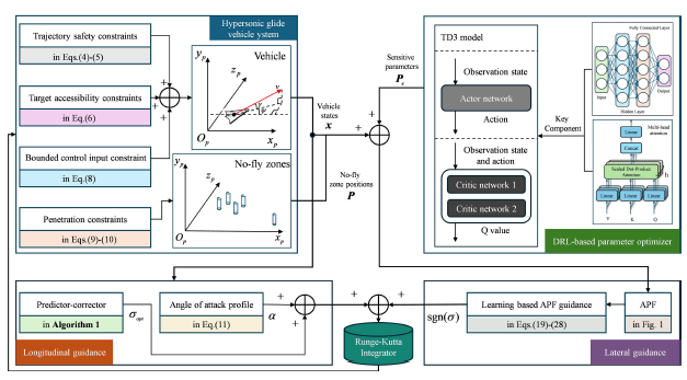
based on the vehicle’s real-time states and surrounding environment. Integrating the mathematical model from Section 2 with the APF-based penetration algorithm in Section 3.1 yields the learning-based APF guidance strategy architecture illustrated in Fig. 2.
The learning-based APF guidance strategy architecture.

Within the proposed learning-based APF penetration guidance framework, a DRL architecture constructs the sensitive parameter optimiser. During each guidance cycle, the optimiser extracts critical features from real-time vehicle states and environmental conditions to determine optimal sensitive parameter sets, constituting a continuous control problem.
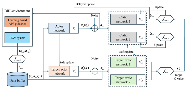
The TD3 algorithm demonstrates exceptional adaptability for continuous control tasks, with core advantages stemming from systematic improvements addressing inherent DRL challenges [Reference Fujimoto, van Hoof and Meger34]. To accommodate high-dimensional continuous action spaces and precision requirements, TD3 employs twin critic networks to mitigate overestimation bias in value functions. Parallel Q-function estimators operate as:
 \begin{align}{y}_{1}=r+\gamma \underset{i=\mathrm{1,2}}{ \min }{Q}_{{{\theta }_{i}^{\prime}}}(s^{\prime},{\pi }_{{\varphi }_{1}}(s^{\prime}))\end{align}
where
 ${y}_{1}$
denotes the target Q-value,
 $r$
is the immediate reward and the
 $ \min $
operator selects conservative value estimates from twin Q-networks.
 $\gamma $
represents the discount factor, while
 ${Q}_{{{\theta }_{i}^{\prime}}}$
corresponds to the target critic network.
Concurrently, delayed policy updates ensure stability in gradient-based policy optimisation, preventing training oscillations caused by frequent policy iterations in conventional methods. Target policy smoothing injects adaptive noise into the action space:
 \begin{align}\tilde{a}={\pi }_{\varphi{'}}\left(s{'}\right)+\varepsilon , \ \ \ \ \varepsilon \sim \mathrm{c}\mathrm{l}\mathrm{i}\mathrm{p}\,(\mathcal{N}(0,{\sigma }^{2}),-c,c)\end{align}
where
 $\tilde{a}$
signifies the noise-injected action,
 ${\pi }_{\varphi{'}}\left(s{'}\right)$
is the action generated by the target policy network and
 $\varepsilon $
truncated Gaussian noise with standard deviation
 $\sigma $
and clipping range
 $[-c,c]$
. The
 $\mathrm{c}\mathrm{l}\mathrm{i}\mathrm{p}({\cdot})$
function ensures noise confinement within physically feasible bounds.
This technique enhances robustness against observational noise and model uncertainties while avoiding local optima during parameter search. Notably, convergence reliability improves significantly in non-convex, multi-extremum optimisation scenarios. Symbols in Equations (29) and (30) maintain consistency with the original literature without conflating with other variables in this work.
Additionally, due to the coupling between the sensitive parameter optimiser and guidance cycles, state data involved in decision-making inherently possesses temporal attributes. Thus, this section incorporates multi-head attention mechanisms from transformer architectures atop fully connected layers to capture contextual relationships among state-space variables for decision support. Multi-head attention demonstrates exceptional efficiency in extracting features from sequential data [Reference Vaswani, Shazeer, Parmar, Uszkoreit, Jones, Gomez, Kaiser and Polosukhin35]. Its core advantage lies in transcending limitations of conventional sequence models through parallelised multi-perspective decomposition and dynamic weight focusing. Temporally, the multi-head structure decomposes hidden representations of input sequences into subspaces, each independently learning distinct temporal dependency patterns. Certain heads focus on feature interactions within local time windows while others capture long-range dependencies across extended periods. This multi-granularity feature decoupling enables simultaneous identification of high-frequency fluctuations and low-frequency trend evolutions in time series. The fundamental computational model of multi-head attention is given by Equation (31).
 \begin{align}\left\{\begin{array}{ll} {} \mathrm{A}\mathrm{t}\mathrm{t}\mathrm{e}\mathrm{n}\mathrm{t}\mathrm{i}\mathrm{o}\mathrm{n}\ (Q,K,V)=\mathrm{s}\mathrm{o}\mathrm{f}\mathrm{t} \max \left(\dfrac{Q{K}^{T}}{\sqrt{{d}_{k}}}\right)V\\[12pt] {} \mathrm{M}\mathrm{u}\mathrm{l}\mathrm{t}\mathrm{i}\mathrm{H}\mathrm{e}\mathrm{a}\mathrm{d}(Q,K,V)=\mathrm{C}\mathrm{o}\mathrm{n}\mathrm{c}\mathrm{a}\mathrm{t}(\mathrm{h}\mathrm{e}\mathrm{a}{\mathrm{d}}_{1},\dots ,\mathrm{h}\mathrm{e}\mathrm{a}{\mathrm{d}}_{h}){W}^{O}\\[3pt] {} \mathrm{w}\mathrm{h}\mathrm{e}\mathrm{r}\mathrm{e} \ \mathrm{h}\mathrm{e}\mathrm{a}{\mathrm{d}}_{i}=\mathrm{A}\mathrm{t}\mathrm{t}\mathrm{e}\mathrm{n}\mathrm{t}\mathrm{i}\mathrm{o}\mathrm{n}\ (Q{W}_{i}^{Q},K{W}_{i}^{K},V{W}_{i}^{V})\end{array}\right. \end{align}
where the parameter matrices
 ${W}_{i}^{Q}\in {\mathbb{R}}^{{d}_{\mathrm{model}}\times {d}_{k}}$
,
 ${W}_{i}^{K}\in {\mathbb{R}}^{{d}_{\mathrm{model}}\times {d}_{k}}$
,
 ${W}_{i}^{V}\in {\mathbb{R}}^{{d}_{\mathrm{model}}\times {d}_{v}}$
and
 ${W}^{O}\in {\mathbb{R}}^{h{d}_{v}\times {d}_{\mathrm{model}}}$
. The number of heads is chosen as
 $h=4$
, and
 ${d}_{k}={d}_{v}={d}_{\mathrm{model}}/h=128$
. The attention function computes a set of queries simultaneously, packing them into matrix
 $Q$
. Correspondingly, keys and values are packed into matrices
 $K$
and
 $V,$
respectively.
In summary, this section designs the agent model for the sensitive parameter optimiser by integrating two key components, fully connected layers and multi-head attention layers, into the TD3-based DRL framework. The training mechanism schematic is shown in Fig. 3, while the structural details of critic and actor networks along with critical parameter designs are specified in Fig. 4.
The training mechanism schematic of the optimiser.

The network structure and key parameters of the optimiser.

Figure 4. Long description
A diagram of the network structure and key parameters of the optimizer. The diagram is divided into three main sections: observation state path, action state path, and critic and actor networks. The observation state path starts with an input layer, followed by a position-embedded layer, self-attention layer with 4 heads, a fully connected layer with 128 neurons, a ReLU layer, a global max pooling layer, and another fully connected layer with 64 neurons. The action state path begins with an input layer, followed by a fully connected layer with 64 neurons, a ReLU layer, another fully connected layer with 128 neurons, a ReLU layer, and a fully connected layer with 64 neurons. The outputs from the observation and action state paths are concatenated and passed through a ReLU layer to produce the final output. The critic network includes layers similar to the observation state path, ending with a fully connected layer with 64 neurons and a Tanh layer for output. The actor network mirrors the critic network structure but ends with a fully connected layer with 8 neurons and a Tanh layer for output.
Following completion of the agent model construction, this section establishes the MDP formulation for the sensitive parameter optimiser as follows.
First, the observation state set must comprehensively encompass the vehicle’s current states and relative situational information regarding targets and environmental factors. Sufficient observations provide essential support for the agent’s optimisation learning and guide effective decision-making. Therefore, the observation state vector
 ${\text{ O}}_{t}$
is defined as:
 \begin{align}\left\{\begin{array}{ll}{\text{ o}}_{t} {} =[r,V,\theta ,\phi ,\psi ,\gamma ,{\Delta }\psi ,{S}_{f,\mathrm{t}\mathrm{o}\mathrm{g}\mathrm{o}},{\Delta }{d}_{r,1},\dots ,{\Delta }{d}_{r,K}{]}^{{\rm T}}\\[4pt] {\text{ O}}_{t} {} =[{\text{ o}}_{t-\tau },\dots ,{\text{ o}}_{t-1},{\text{ o}}_{t}{]}^{{\rm T}}\end{array}\right.\end{align}
where
 ${\text{ o}}_{t}$
denotes the state vector at time
 $t$
,
 $r,V,\theta ,\phi ,\psi ,\gamma $
represents the vehicle’s flight states,
 ${\Delta }\psi ,{S}_{f,\mathrm{t}\mathrm{o}\mathrm{g}\mathrm{o}}$
indicates positional deviation from the target,
 ${\Delta }{d}_{r,1}, \ldots ,{\Delta }{d}_{r,K}$
corresponds to relative distances between the vehicle and centroids of NFZs with size
 $K=5$
, and
 $\tau =5$
signifies the temporal dimension of the observation state vector set.
Remark 2. The underlying design logic and physical insights of the observation vector
 ${\text{ O}}_{t}$
are elaborated from three aspects to provide comprehensive context for policy optimisation: first, to satisfy the Markov property required for reinforcement learning, the basic motion states (
 $r,V,\theta ,\phi ,\psi ,\gamma $
) are incorporated to strictly represent the vehicle’s instantaneous operational status. Second, to steer the agent to satisfy both terminal guidance objectives and spatial safety constraints, task-oriented features are embedded. Specifically,
 ${\Delta }\psi $
and
 ${S}_{f,\mathrm{t}\mathrm{o}\mathrm{g}\mathrm{o}}$
represent the directional and range-to-go errors, offering direct gradients for terminal convergence. Meanwhile, the relative distances
 ${\Delta }{d}_{r,k}$
(
 $k=1,\dots ,K$
) map the explicit spatial relationships between the vehicle and multiple NFZs, ensuring that the learned policy can proactively execute avoidance manoeuvres prior to boundary violations. Third, to mitigate the adverse effects of partial observability in complex flight environments, a temporal sequence structure with a history window of
 $\tau =5$
is constructed. Stacking these historical observation frames allows the deep neural network to implicitly capture the temporal variations and higher-order derivatives of the vehicle’s motion states. This temporal depth significantly stabilises the reinforcement learning training process and enhances the robustness of the derived cooperative guidance law under dynamic environments.
The action space design aligns with the sensitive parameter set as follows:
 \begin{align}\text{ a}=\left\{{\Delta }{\psi }_{buff},{K}_{gra},{K}_{rep},{\rho }_{k}|k=\mathrm{1,2},\dots ,K\right\}\end{align}
where parameters in the action space are bounded within loose boundaries determined through offline testing and analysis. This study selects
 ${\Delta }{\psi }_{buff}\in [2.{5}^{\circ },7.{5}^{\circ }]$
,
 ${K}_{gra}\in [1\times 1{0}^{3},9\times 1{0}^{3}]$
,
 ${K}_{rep}\in [5\times 1{0}^{3},1\times 1{0}^{4}]$
,
 ${\rho }_{k}\in [1\times 1{0}^{6},2\times 1{0}^{6}]$
.
The reward function designed in this study comprises process rewards and terminal rewards, with process rewards consisting of safety reward
 ${R}_{s,k}$
and flight reward
 ${R}_{f}$
.
-
(1) Safety reward serves as the primary feedback to guide the agent toward decisions maintaining safe distances from NFZs, which is critical for fulfilling fundamental avoidance requirements The core principle of
${R}_{s,k}$
involves regulating the relative distance between the vehicle and NFZ centroids, categorised into danger zones (
${\Delta }{d}_{r,k}\le {R}_{N,k}$
), strong penalty zones (
${R}_{N,k}\lt \Delta {d}_{r,k}\le 1.1{R}_{N,k}$
), alert zones (
$1.1{R}_{N,k}\lt \Delta {d}_{r,k}\le 1.2{R}_{N,k}$
) and safe zones. Gradient-based designs corresponding to each category guide rational decision-making: (a) danger zones impose substantial fixed penalties and terminate episodes; (b) strong penalty zones apply exponential penalties to drive rapid evasion; (c) alert zones enforce linear penalties to promote gradual distancing; (d) safe zones incur no penalties. -
(2) Flight reward
${R}_{f}$
relates to spherical distance between the vehicle and target terminal along with flight duration, ensuring adherence to target reachability constraints while avoiding sparsity issues inherent in terminal-only rewards.
${R}_{f}$
primarily governs flight time and remaining range, incentivising target-approaching strategies. -
(3) Terminal reward
${R}_{goal}$
provides one-time rewards based on whether preset terminal states are achieved upon episode completion.


Mathematical formulations of these reward functions are defined below:
 \begin{align}{R}_{s,k}=\begin{cases}-{\lambda }_{1}, {} & \mathrm{i}\mathrm{f}\ {\,\tilde{\!d}}_{k}\le 1\\[3pt] -{\lambda }_{2}\exp ({\lambda }_{3}(1-{\,\tilde{\!d}}_{k})), {} &\mathrm{i}\mathrm{f} \ 1\lt {\,\tilde{\!d}}_{k}\le 1.1\\[3pt] -{\lambda }_{4}(1.2-{\,\tilde{\!d}}_{k}), & {} \mathrm{i}\mathrm{f} \ 1.1\lt {\,\tilde{\!d}}_{k}\le 1.2\\[3pt] 0, & {} \mathrm{otherwise}\end{cases}\end{align}
where
 $\ {\,\tilde{\!d}}_{k}={\Delta }{d}_{r,k}/{R}_{N,k}$
denotes the normalised distance.
 \begin{align}{R}_{f} &=-{\lambda }_{5}({S}_{f,\mathrm{t}\mathrm{o}\mathrm{g}\mathrm{o}}-{L}_{r,f})/(t\cdot {L}_{r,f}) \\[-28pt] \nonumber \end{align}
 \begin{align} \qquad {R}_{\mathrm{g}\mathrm{o}\mathrm{a}\mathrm{l}} &=\begin{cases}{\lambda }_{6}, & \mathrm{i}\mathrm{f} \ \mathrm{E}\mathrm{q}.\left(6\right) \ \mathrm{i}\mathrm{s} \ \mathrm{s}\mathrm{a}\mathrm{t}\mathrm{i}\mathrm{s}\mathrm{f}\mathrm{i}\mathrm{e}\mathrm{d}\\[3pt] -{\lambda }_{7}, & {} \mathrm{otherwise}\end{cases}\end{align}
where
 ${\lambda }_{1}-{\lambda }_{7}$
denote configurable parameters, and
 $t$
represents flight time.
Consequently, the total reward guiding agent policy optimisation is:
 \begin{align}{R}_{w}=\sum _{k=1}^{K}{R}_{s,k}+{R}_{f}+{R}_{\mathrm{g}\mathrm{o}\mathrm{a}\mathrm{l}}\end{align}
Remark 3. Reward functions in Equations (34)–(36) require rational parameter configurations to ensure efficient environmental responses and dynamic multi-objective balance. First, mathematical continuity at segment boundaries of the safety reward must be preserved to avoid abrupt reward changes during boundary transitions. However, stepwise penalties remain permissible for catastrophic failures to deter unacceptable behaviours. Second, magnitude coordination among reward functions is essential for balanced multi-objective optimisation. Based on these considerations and real-time adjustments from training feedback, this study selects:
 ${\lambda }_{1}=25$
,
 ${\lambda }_{2}=22.5$
,
 ${\lambda }_{3}=30$
,
 ${\lambda }_{4}=11.25$
,
 ${\lambda }_{5}=0.025$
,
 ${\lambda }_{6}=5000$
,
 ${\lambda }_{7}=10,000$
.
Following agent model construction and MDP formulation for the sensitive parameter optimiser, policy learning proceeds according to the Fig. 3 training mechanism with key parameters configured in Table 1.
Key parameter specifications for agent training

Table 1. Long description
A table titled ‘Parameters’ and ‘Settings’ with two columns and 14 rows. The first column lists the parameters, and the second column lists their corresponding settings. The parameters include Observation space dimension, Action space dimension, Learning rate of actor, Learning rate of critic, L2 regularisation factor of actor, L2 regularisation factor of critic, Optimiser, Attention head count, Target smooth factor, Gradient threshold, Discount factor, Variance of target policy smooth model, Lower limit of target policy smooth model, and Upper limit of target policy smooth model. The settings for these parameters are 13 x 5, 8 x 1, 1e - 3, 2e - 4, 1e - 5, 2e - 4, Adam, 4, 5e - 3, 1, 0.99, 0.2, -0.5, and 0.5 respectively.
In summary, the learning-based artificial potential field guidance strategy for HGV penetration has been established.
4.0 Numerical simulations
To validate the efficacy of the learning-based artificial potential field guidance strategy established in Section 3 for penetration scenarios, a series of numerical simulations were conducted using MATLAB 2023b on a computational platform (AMD Ryzen 7 4800H, 2.9 GHz). Detailed parameter configurations, visualised experimental results, and corresponding analyses are provided to ensure simulation reliability and reproducibility.
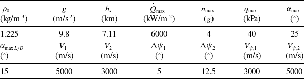
First, the penetration scenario incorporates five NFZs with deployment positions and influence radii configured as specified in Table 2. Second, rigidly constrained trajectory endpoints for the HGV mission are defined in Table 3. Finally, parameters governing the penetration guidance strategy in Section 3 are detailed in Table 4.
Configurations for joint NFZs

Table 2. Long description
A table detailing the configurations for joint No-Fly Zones (NFZs) with specific positions and radii. The table has five rows and three columns. The columns are labeled NFZs, Position (E, N), and Radius R_N (km). The rows provide specific details for each NFZ. Row 1: NFZs #1, Position (37.5, 6.0), Radius 225 km. Row 2: NFZs #2, Position (32.5, 0.0), Radius 225 km. Row 3: NFZs #3, Position (25.0, 4.0), Radius 225 km. Row 4: NFZs #4, Position (45.0, 2.0), Radius 225 km. Row 5: NFZs #5, Position (52.5, 5.0), Radius 50 km.
Initial and terminal state settings of HGV

Table 3. Long description
A table comparing initial and terminal state settings of HGV. The table has 10 columns and 2 rows. The columns are labeled as follows: h_0 (km), V_0 (m/s), θ_0 (°), φ_0 (°), ψ_0 (°), γ_0 (°), h_f (km), V_f (m/s), θ_f (°), φ_f (°), and L_R,f (km). The first row contains the following values: 60, 7000, 0, 0, 90, 0, 27, 1550, 55, 5, and 100. The second row is empty.
Parameter configuration for the guidance strategy

Table 4. Long description
A table detailing parameters for a guidance strategy. The table has 12 columns and 2 rows. Column headers are: rho subscript 0, g, h subscript f, Q subscript max, n subscript max, q subscript max, alpha subscript max, alpha subscript max L/D, V subscript 1, V subscript 2, Delta psi subscript 1, Delta psi subscript 2, V subscript psi 1, V subscript psi 2. Row 1: rho subscript 0, 1.225 kg/m^3; g, 9.8 m/s^2; h subscript f, 7.11 km; Q subscript max, 6000 kW/m^2; n subscript max, 4 g; q subscript max, 40 kPa; alpha subscript max, 25 degrees; alpha subscript max L/D, 15 degrees; V subscript 1, 5000 m/s; V subscript 2, 3000 m/s; Delta psi subscript 1, 5 degrees; Delta psi subscript 2, 12.5 degrees; V subscript psi 1, 3000 m/s; V subscript psi 2, 5000 m/s.
4.1 Agent training for sensitive parameter optimisation
Building upon the agent architecture, reward mechanisms and training framework established in Section 3, this section conducts agent training for sensitive parameter optimisation. The offline training incorporates comprehensive uncertainties and dispersion errors inherent to HGV systems to enhance the generalisation capability of the DRL method and ensure operational effectiveness of the trained actor network. As detailed in Table 5, aerodynamic model uncertainties and initial state dispersion errors follow uniform distributions calibrated to actual flight system characteristics.
Uniform distributions for aerodynamic uncertainties and initial state dispersions

Table 5. Long description
A table showing uniform distributions for aerodynamic uncertainties and initial state dispersions. The table has 1 row and 9 columns. The columns are labeled as follows: h subscript 0 (km), V subscript 0 (m/s), theta subscript 0 (degrees), phi subscript 0 (degrees), psi subscript 0 (degrees), gamma subscript 0 (degrees), m subscript 0 (kg), C subscript L, C subscript D, and rho. The values in the table are as follows: Row 1: h subscript 0, plus or minus 1; V subscript 0, plus or minus 50; theta subscript 0, plus or minus 1; phi subscript 0, plus or minus 1; psi subscript 0, plus or minus 0.5; gamma subscript 0, plus or minus 0.1; m subscript 0, plus or minus 5 percent; C subscript L, plus or minus 10 percent; C subscript D, plus or minus 10 percent; rho, plus or minus 10 percent.
The model training encompasses 1500 episodes. To accelerate exploration of efficient decision policies during initial training phases and mitigate early-stage instability, environment states are initialised with fixed random seeds until significant convergence trends emerge in reward curves. This strategy provides a controlled starting point while reducing stochastic interference during exploratory phases. Upon observing definitive convergence trends in later training stages, the environment initialisation shifts to randomised reset mode, employing dynamically varying random seeds. This introduces environmental uncertainties to evaluate and enhance agent robustness and adaptability under noisy or perturbed conditions. The episodic reward and its moving average throughout training are depicted in Fig. 5.
Reward curves for agent training in sensitive parameter optimisation.

Figure 5. Long description
A line graph showing the reward curves for agent training in sensitive parameter optimization. The horizontal axis represents the episode number, ranging from 0 to 1500. The vertical axis represents the episode reward, ranging from -12000 to 6000. The graph includes three data lines: one for episode reward, one for average reward, and one for the episode number of environment reset. The episode reward line fluctuates significantly in the beginning, showing large spikes and drops. Around episode number 200, the episode reward stabilizes and starts to increase steadily. The average reward line shows a smoother increase over time, indicating the agent’s learning progress. Vertical dashed lines mark the episodes where the environment is reset, occurring at approximately episodes 1000, 1100, 1200, 1300, and 1400. The episode reward line stabilizes around 4000 after episode number 600, indicating the agent has learned to achieve consistent high rewards.
Figure 5 distinctly reveals the agent’s learning dynamics. During the initial training phase (first 1000 episodes), the agent operates in an exploration-dominated period. At this stage, limited policy experience results in highly stochastic behaviours that frequently trigger environmental penalties, causing substantial episodic reward fluctuations with pronounced oscillations. As training progresses and policy networks undergo iterative optimisation, the agent progressively learns decision patterns that maximise cumulative rewards by identifying and avoiding hazardous states while pursuing high-reward actions. This capability to construct effective internal representations of environmental dynamics and generate adaptive responses remains robust after introducing dynamically randomised environment resets in later training stages (post-1000 episodes). Confronting abrupt environmental uncertainties and state-space perturbations, the agent rapidly adjusts strategies while maintaining decision robustness and efficiency. Therefore, the final performance demonstrates: (a) significantly reduced fluctuation of episodic rewards with converging distribution stability; (b) progressive improvement in mean reward culminating in statistically significant convergence.
These systemic transformations collectively demonstrate successful acquisition of a stable, adaptive and efficient policy resilient to dynamically evolving environments.
Comparative simulation results.

4.2 Effectiveness validation of learning-based APF guidance strategy
To verify the effectiveness and superiority of the proposed learning-based APF guidance strategy in practical flight missions, this section conducts both ablation studies and comparative simulation experiments under standard conditions. The algorithm employed for the ablation study is the APF guidance strategy configured with a fixed sensitive parameter set. To ensure a fair comparison, this parameter set has undergone rigorous offline tuning to ensure its fundamental suitability for the specified flight mission. Furthermore, to evaluate the performance of the proposed algorithm relative to other mainstream evasive guidance methods, the IFDS algorithm is selected as the benchmark based on a comprehensive literature review. Since both the IFDS and the APF belong to the category of field-theory-based algorithms, they adhere to the principle of fairness for comparative analysis. Finally, the performance of these three algorithms is analysed and compared based on multiple evaluation metrics. The key parameters for constructing the flight mission environment are detailed in Tables 2 and 3, while the configurable parameters involved in the aforementioned algorithms are specified in Table 4. The simulation results are presented in Figs. 6 and 7 and Table 6, and the detailed analysis and corresponding conclusions are provided as follows:
Terminal states in the comparative simulations

Table 6. Long description
A table comparing the performance metrics of three algorithms: Learning-APF, APF, and IFDS. The table has four rows and five columns. The columns are labeled as Algorithm, hf/km, Vf/(m/s), Lrj/km, and tf/s. Each row provides specific values for these metrics. Row 1: Learning-APF, hf/km 26.13 (-3.22 percent), Vf/(m/s) 1554.70 (+0.30 percent), Lrj/km 100.56 (+0.56 percent), tf/s 2.014. Row 2: APF, hf/km 26.38 (-2.30 percent), Vf/(m/s) 1556.37 (+0.41 percent), Lrj/km 101.35 (+1.35 percent), tf/s 1.215. Row 3: IFDS, hf/km 27.41 (+1.52 percent), Vf/(m/s) 1553.23 (+0.21 percent), Lrj/km 101.24 (+1.24 percent), tf/s 0.816. The table provides a detailed comparison of the performance metrics for each algorithm, highlighting differences in their effectiveness and efficiency.
The minimum distance between the vehicle and NFZs.

-
(1) Figure 6a illustrates the ground trajectories calculated by the three guidance algorithms. Combined with the statistical analysis of the minimum relative distance between the vehicle and the NFZs presented in Fig. 7, it is evident that the vehicles guided by all three algorithms are capable of penetrating the joint NFZ blockade and reaching the designated terminal point. However, due to the distinct intrinsic attributes and parameter configurations of each algorithm, the generated evasive strategies exhibit significant differences under identical environmental constraints.
-
(2) The curves in Fig. 6b indicate that all three algorithms achieve successful penetration guidance while satisfying the re-entry flight corridor constraints defined in Equation (4). According to EqUationss (12) and (13), the flight corridor constraints composed of process constraints are transformed into amplitude constraints on the bank angle within the longitudinal guidance cycle. Since these three algorithms employ distinct lateral guidance strategies yet share the same longitudinal guidance framework, these results fully demonstrate the robustness of the longitudinal guidance design proposed in this study.
-
(3) Figure 6c illustrates the bank angle commands generated by the three algorithms, which are directly correlated with their respective evasive strategies. Specifically, the bank angle manoeuvre pattern of the learning-based APF guidance strategy achieves safe penetration with fewer reversals, thereby further ensuring the stability of the flight trajectory. Moreover, the IFDS algorithm exhibits severe oscillations in heading correction, which further validates the necessity of the buffer zone setting and its rational parameter configuration. Adopting the contact with the NFZ boundary as the sole correction criterion leads to a rapid correction-hold-correction cycle once the vehicle approaches the tangent direction of the NFZ, continuing until the vehicle exits the influence range of the NFZ.
-
(4) To provide a clearer depiction of the heading correction details for the three guidance algorithms, Fig. 6d presents the heading angle error curves under the lateral heading error corridor constraints. It is worth noting that this error corridor functions as an elastic soft constraint rather than a rigid hard boundary; its primary purpose is to provide corrective regulation whenever a large deviation occurs between the heading angle and the line-of-sight direction to the target. During the midcourse flight, transient excursions beyond this preset corridor are acceptable, as the vehicle must balance the trade-off between two competing objectives, namely obstacle avoidance and terminal reachability. Different avoidance manoeuvres inherently yield varying heading profiles, which merely reflect the distinct manoeuvring strategies adopted by each algorithm. Figure 6d clearly demonstrates that all three methods rigorously fulfill the final terminal heading requirements. Nevertheless, it should be emphasised that both APF-based algorithms are capable of maintaining relatively linear and gradual heading error profiles. As a comparison, the guidance strategy based on IFDS suffers from noticeable fluctuations in heading tracking, as shown in Fig. 6c. Such behaviour reveals that the IFDS framework struggles to balance obstacle avoidance against destination reachability, inducing undesirable trajectory oscillations and compromising the system’s safety margin. In contrast, the algorithm developed in this task achieves the desired guidance commands with fewer heading corrections, ensuring higher trajectory stability.
-
(5) Table 6 presents the performance of the three algorithms in terms of the terminal constraint set and execution time. Since the evasive guidance strategy prioritises the handling of path constraints during flight, and all three algorithms share the same fundamental guidance framework, they exhibit similarly high precision in satisfying terminal constraints. It should be noted that the learning-based APF guidance strategy entails a higher computational overhead due to the requirements of network model loading and forward propagation. Compared with the IFDS algorithm, the proposed APF requires more nested decision-making and related calculations rather than simple physics-based heading computations, which is due to several specific designs tailored for compatibility with the re-entry flight process. Consequently, this leads to a longer solution time. Nevertheless, on the premise of ensuring trajectory reliability and safety, the overall time cost has not increased significantly. Specifically, it should be clarified that the time statistics presented in Table 6 denote the cumulative computational duration required for the complete trajectory generation. For this specific trajectory, the average single-step execution time of the proposed algorithm is calculated as approximately
$1.458 \ \mathrm{m}\mathrm{s}$
. According to the state-of-the-art intelligent entry guidance framework [Reference Cheng, Jiang, Wang and Li36], the authoritative real-time execution limit for onboard flight computers is established at
$50 \ \mathrm{m}\mathrm{s}$
per control cycle (corresponding to a
$20 \ \mathrm{H}\mathrm{z}$
command update frequency). Manifestly, the single-step latency of the proposed strategy (
$1.458 \ \mathrm{m}\mathrm{s}$
) is well within this required
$50 \ \mathrm{m}\mathrm{s}$
ceiling, completely satisfying the onboard real-time standard with an ample safety margin.


4.3 Monte Carlo results
To further verify the anti-disturbance capability and adaptability of the learning-based APF guidance strategy in an uncertain environment, and to simultaneously highlight the advantages of the sensitive parameter optimiser over fixed parameter sets under disturbances to environmental and mission parameters through comparison, this section conducts 500 independent and repeated shooting simulation experiments for each of the three algorithms. The experiments refer to the parameter settings in Table 5 and control the random number seeds within the range of 1–500. The statistical results of the simulations are presented in Figs. 8 and 9 and Tables 7 and 8, and the detailed analysis and corresponding conclusions are provided as follows:
Terminal statistical results of successful cases in Monte Carlo experiments

Table 7. Long description
A table comparing the performance of three algorithms in Monte Carlo experiments. The table has four rows and four columns. The columns are labeled h_i (percent), V_i (percent), L_rj (percent), and p_su (percent). The rows are labeled Learning-APF, APF, and IFDS. Row 1: Learning-APF, h_i 2.64 ± 1.33, V_i 0.21 ± 0.16, L_rj 0.77 ± 0.46, p_su 99.2. Row 2: APF, h_i 2.71 ± 1.59, V_i 0.21 ± 0.15, L_rj 0.80 ± 0.43, p_su 76.2. Row 3: IFDS, h_i 6.58 ± 0.88, V_i 0.47 ± 0.14, L_rj 0.82 ± 0.46, p_su 65.6. The table presents statistical results of successful cases in Monte Carlo experiments, highlighting the performance metrics of each algorithm.
Ground trajectories of the Monte Carlo experiments.

Comparative results of policy inference efficiency

Table 8. Long description
A table comparing the memory usage and inference time of three algorithms. The table has three rows and four columns. The columns are labeled Algorithm, Total memory (MB), Peak memory (MB), and Inference time (s). The row labels are Learning-APF, APF, and IFDS. Row 1: Learning-APF, Total memory 125.151 MB plus or minus 11.746 MB, Peak memory 4.012 MB plus or minus 0.001 MB, Inference time 2.059 seconds plus or minus 0.104 seconds. Row 2: APF, Total memory 24.149 MB plus or minus 5.675 MB, Peak memory 2.484 MB plus or minus 0.166 MB, Inference time 1.280 seconds plus or minus 0.026 seconds. Row 3: IFDS, Total memory 27.371 MB plus or minus 4.868 MB, Peak memory 2.505 MB plus or minus 0.002 MB, Inference time 0.829 seconds plus or minus 0.022 seconds.
Comparative results of penetration probability.

-
(1) Analysis of Fig. 8a, b and e reveals that even under identical environmental settings, the strategies employed by the three algorithms to achieve successful penetration differ significantly. The learning-based APF strategy flexibly selects evasive manoeuvres according to the vehicle’s proximity to NFZs, which significantly enhances the smoothness of the generated trajectories. In contrast, the APF algorithm with fixed parameters and the IFDS algorithm exhibit more rigid planning behaviours, as their fixed configurations fail to generate effective adaptive responses when encountering environmental disturbances.
-
(2) As illustrated in Fig. 8b, d and f, the learning-based APF outperforms the other two algorithms with the lowest number of failure cases. The primary obstacles leading to failures in both the fixed APF and IFDS are the two NFZs encountered during the early flight stage. This phenomenon is attributed to the hypersonic speeds, large turning radii and limited heading adjustment capacity during this period, which necessitate a higher redundancy margin in the evasive strategy. However, the fixed APF cannot adaptively adjust its strategy based on early flight requirements, while the IFDS, relying solely on physical constraints, neglects the specific demands of the re-entry process.
-
(3) To provide a clearer representation of the performance differences in Monte Carlo simulations, Fig. 9 summarises the penetration success rates for the joint NFZs. It must be acknowledged that the learning-based APF does not achieve a 100% success rate, as shown in Fig. 8b. This is closely related to factors such as the inherent capacity boundaries of the algorithm and the need for further refinement in parameter optimisation. Nevertheless, the learning-based APF demonstrates superior robustness against environmental disturbances. Under the same experimental conditions, the proposed strategy increases the success rate from 76.2% (fixed APF) to 99.2%, significantly exceeding the 65.6% success rate of the IFDS.
-
(4) The terminal control precision for all successful cases in the Monte Carlo simulations is summarised in Table 7. The data indicate that although the three algorithms share the same basic guidance framework, the lateral errors caused by different evasive strategies must be compensated for within the longitudinal guidance loop. The flexibility of the learning-based APF further releases the control margin for longitudinal guidance, thereby achieving higher terminal control precision.
-
(5) To further investigate the computational costs on hardware platforms, the memory consumption (including total and peak consumption) and execution time for all test cases are recorded. The analysis of Table 8 shows that compared to the purely mathematical APF and IFDS algorithms, the learning-based APF incurs higher memory and time costs. These are necessary overheads resulting from agent model loading and network forward propagation. Nevertheless, these costs remain well within the operational load requirements of general hardware development platforms.
In summary, the learning-based APF guidance strategy proposed in this study can achieve a better balance between target reachability and penetration. It can also significantly improve the rigidity of penetration strategies caused by fixed parameters, all while not compromising terminal control precision or operation time. Therefore, it serves as a more efficient and robust penetration strategy.
5.0 Conclusion
This study addresses the penetration guidance challenge of HGVs in joint NFZs under complex constrained environments, with key conclusions summarised as follows: first, the APF method effectively resolves the inherent contradictions of integrating traditional artificial potential field methods into the HGV penetration guidance framework. It establishes a reasonable reference heading mechanism for obstacle environments, laying a technical foundation for subsequent optimisation and providing a reliable comparison benchmark. Second, the online parameter optimiser is designed based on the multi-head self-attention mechanism and TD3 DRL framework, and it exhibits strong adaptive adjustment capabilities. By leveraging time-series state data to perceive environmental dynamics, the optimiser generates real-time evasion strategy responses. This overcomes the limitations of manual offline adjustment and the rigidity of fixed online strategies. Additionally, the three designed reward function models avoid sparse rewards in reinforcement learning, ensuring stable convergence of the agent’s strategy learning. Third, ablation studies and comparative experiments confirm the effectiveness and robustness of the proposed learning-based APF guidance framework. Under both standard and environmental disturbance conditions, the framework maintains high terminal control precision and operational efficiency. It also balances target reachability with penetration success, and significantly enhances strategy flexibility and adaptability to uncertain environments compared to fixed-parameter strategies. In conclusion, this learning-based evasion guidance framework offers a new technical approach for improving HGVs’ penetration capability in complex environments. However, a potential limitation lies in the framework’s generalisation boundaries under extreme, unmodeled environmental anomalies, and the continuous parameter adaptation may incur additional computational overhead. Future research may expand environmental disturbance scenarios or optimise the reinforcement learning network structure to enhance real-time performance and generalisation for more challenging flight conditions.
Acknowledgements
This work was supported in part by the Key Program of National Natural Science Foundation of China under Grant U24B20177, in part by State Key Laboratory of High-Efficiency Reusable Aerospace Transportation Technology, and in part by Beijing Key Laboratory of System Design for Reusable Launch Vehicle.

 |σopt|