1 Introduction
Intrinsic steady-state and disruption-free operations and lack of a density limit are some of the significant advantages of stellarators over tokamaks. However, the fully three-dimensional nature of stellarator geometries introduces several mathematical, physical and engineering challenges (Helander et al. Reference Helander, Beidler, Bird, Drevlak, Feng, Hatzky, Jenko, Kleiber, Proll and Turkin2012; Helander Reference Helander2014). The theory of magnetohydrodynamic (MHD) equilibrium and vacuum magnetic fields in a non-symmetric torus with nested flux surfaces or closed magnetic field lines is far from understood (Newcomb Reference Newcomb1959; Grad Reference Grad1967; Weitzner Reference Weitzner2014, Reference Weitzner2016; Hudson & Kraus Reference Hudson and Kraus2017; Sengupta & Weitzner Reference Sengupta and Weitzner2019). Broadly, there are three kinds of vacuum or equilibrium magnetic field lines relevant to toroidal confinement, namely, ergodic field lines on nested flux surfaces, ergodic volume filling field lines and closed field lines. Ergodic field lines lying on flux surfaces only occur in magnetic field-line systems that are integrable (Cary & Littlejohn Reference Cary and Littlejohn1983) when the rotational transform is irrational. In the absence of any continuous symmetry, the magnetic field-line system is, in general, chaotic, and the field lines are ergodic and volume filling. Closed magnetic fields are found in systems with continuous symmetries when the rotational transform is rational (Newcomb Reference Newcomb1959), as well as in non-symmetric systems with discrete symmetries (Lortz Reference Lortz1970; Grad Reference Grad1971). The only rigorous example of an ideal MHD equilibrium without any continuous symmetry is given by Lortz (Reference Lortz1970). He proved that, in a system with reflection symmetry, a non-symmetric three-dimensional MHD equilibrium with a smooth pressure profile can be constructed iteratively starting with a vacuum field with closed field lines and zero shear. A significant drawback of this result is that the rotational transform for such an equilibrium is zero. Weitzner and Sengupta (2019) derived exact analytical expressions for vacuum magnetic fields with closed field lines in a flat toroidal shell (a topological torus) and extended Lortz’s result to include all rational rotational transform.
Given non-symmetric equilibrium or vacuum fields with approximately nested surfaces, radial confinement of particles trapped in these fields cannot be guaranteed. It is well known that particle orbits in perfectly axisymmetric magnetic fields are bounded radially. In non-axisymmetric magnetic fields with nested flux surfaces, circulating particle orbits are radially bounded. In contrast, trapped particles generally have trajectories that gradually drift out from the confined region outward to open field lines within a few bounce times. The neoclassical particle and energy fluxes associated with these unconfined orbits can be significant for un-optimized stellarators (Mynick Reference Mynick2006). Various properties of the magnetic field such as quasisymmetry (Nührenberg & Zille Reference Nührenberg and Zille1988; Boozer Reference Boozer1995), quasi-axisymmetry (Nührenberg et al. Reference Nührenberg, Sindoni, Lotz, Troyon, Gori and Vaclavik1994; Okamura et al. Reference Okamura, Matsuoka, Nishimura, Isobe, Nomura, Suzuki, Shimizu, Murakami, Nakajima and Yokoyama2001), omnigeneity (Hall & McNamara Reference Hall and McNamara1975; Cary & Shasharina Reference Cary and Shasharina1997a) and quasi-isodynamicity (Gori, Lotz and Nührenberg Reference Gori, Lotz and Nührenberg1996; Nührenberg Reference Nührenberg2010) have been proposed to reduce the radial drifts.
The theory of single-particle motion shows that the secular radial drift of particles is absent in magnetic field systems with nested flux surfaces when the second adiabatic invariant  $J_{\Vert }=\oint v_{\Vert }\,\text{d}l$, where
 $v_{||},\text{d}l$ are the particle speed and line element along the field line, is independent of the magnetic field-line label on a given flux surface. Omnigeneity is defined as configurations where surfaces of constant
 $J_{\Vert }$, the drift surfaces, are also flux surfaces (Cary & Shasharina Reference Cary and Shasharina1997b). Quasisymmetry (QS) can be shown to be a particular case of omnigeneity (Landreman & Catto Reference Landreman and Catto2012). Through a local expansion near a minimum of the magnetic field, strength (Sengupta & Weitzner Reference Sengupta and Weitzner2018) shows that it is easier to satisfy the omnigeneity condition than the quasisymmetry requirement. Furthermore, the QS constraint makes the MHD system overdetermined, and in general, such magnetic fields might not exist except on isolated surfaces (Garren & Boozer Reference Garren and Boozer1991; Landreman & Sengupta Reference Landreman and Sengupta2018; Landreman, Sengupta & Plunk Reference Landreman, Sengupta and Plunk2019; Landreman & Sengupta Reference Landreman and Sengupta2019). Lack of QS in a volume particularly reduces the confinement of
 $\unicode[STIX]{x1D6FC}$ particles (Bader et al. Reference Bader, Drevlak, Anderson, Faber, Hegna, Likin, Schmitt and Talmadge2019). While the search for finding exact QS in a volume is still ongoing (Burby, Kallinikos & MacKay Reference Burby, Kallinikos and MacKay2019), it has been shown that QS can be satisfied on one surface (Garren & Boozer Reference Garren and Boozer1991; Plunk & Helander Reference Plunk and Helander2018; Henneberg, Drevlak & Helander Reference Henneberg, Drevlak and Helander2019).
In this work, we study charged particle dynamics in a vacuum magnetic field with closed field lines (Weitzner & Sengupta Reference Weitzner and Sengupta2020) and X-points. We restrict ourselves to a flat toroidal shell (a topological torus), which addresses all the complexities arising from the doubly periodic nature of the toroidal domain without the complexities associated with the toroidal curvature. The model magnetic field has all closed field lines with zero shear and reflection symmetries. Modern stellarators experiments like the high- configuration of W7-X (Andreeva Reference Andreeva2002; Klinger et al. Reference Klinger, Andreeva, Bozhenkov, Brandt, Burhenn, Buttenschön, Fuchert, Geiger, Grulke and Laqua2019) can have very low global magnetic shear and a rotational transform close to a low-order rational number. Experimental results from Wendelstein VII-A/AS (Brakel et al. Reference Brakel, Anton, Baldzuhn, Burhenn, Erckmann, Fiedler, Geiger, Hartfuss, Heinrich and Hirsch1997; Brakel & the W7-AS Team Reference Brakel2002; Hirsch et al. Reference Hirsch, Baldzuhn, Beidler, Brakel, Burhenn, Dinklage, Ehmler, Endler, Erckmann and Feng2008) and numerical results (Wobig Reference Wobig1987; Andreeva Reference Andreeva2002) support the idea that optimum confinement is usually found close to certain low-order rational surfaces.
Since rational surfaces where the field lines close on themselves are measure zero compared to irrational surfaces in integrable magnetic field systems, it is tacitly assumed in most QS and omnigeneity analysis that the field lines are ergodic on the flux surfaces. In this work, we formulate and analyse the closed field-line versions of the radial confinement schemes without the assumption of any continuous symmetry. In particular, we explore the relation between drift surfaces and pressure surfaces in closed field-line systems. In such systems, pressure surfaces are labelled by surfaces of constant  $q=\oint \text{d}l/B$ (Grad Reference Grad1971), where
 $B$ is the magnetic field strength, and the integration is carried out along a closed field line. In contrast to MHD equilibrium with irrational rotational transform, pressure surfaces in closed field-line systems are not necessarily functions of only one Clebsch variable. Hence, a proper distinction must be made between radial confinement strategies for systems with rational and irrational rotational transforms. We construct explicit examples to compare and contrast the omnigeneity and QS definitions for closed field lines and ergodic field lines on flux surfaces. In particular, we show that even though the system is not omnigeneous or QS according to the standard definitions for irrational surfaces, the drift surfaces for all particles can coincide with pressure surfaces (
 $q$ surfaces), making the system omnigeneous. This has implications for the particle dynamics near the X-point as well. Through an explicit calculation of the lowest-order drift surfaces, we show that the constant
 $q$ surfaces play a critical role in determining the particle drifts near the X-points. Since QS and omnigeneity, in general, cannot be exactly satisfied, it does not matter if the drift surfaces (
 $\oint \text{d}lv_{\Vert }$) and the
 $q$ surfaces (
 $\oint \text{d}l/B$) surfaces do not coincide to higher orders (BenDaniel Reference BenDaniel1965; Grad Reference Grad1967). Therefore, the lowest-order asymptotic analysis can provide valuable insight into the collisionless cross-field drifts of particles in systems with very long connection lengths.
The outline of the paper is as follows. In § 2, we shall discuss the concepts of omnigeneity and quasisymmetry in the magnetic field system with closed field lines. In § 3, we shall discuss the model magnetic field with closed field lines and evaluate the omnigeneity and quasisymmetry constraints. We shall compare the lowest-order drift surfaces with the constant  $q$ surfaces and the Clebsch flux variable. For the model magnetic, the lowest-order drift surfaces are shown to coincide with the constant
 $q$ surfaces. Finally, we shall discuss the implications of our results in § 4.
2 Omnigeneity and quasisymmetry for magnetic field systems with closed field lines
There are many intrinsic differences between ideal MHD equilibrium with closed magnetic field lines and equilibrium with ergodic field lines that lie on nested flux surfaces (Grad Reference Grad1971). For ergodic field lines with flux surfaces, pressure surfaces coincide with the flux surfaces. For closed field lines, pressure surfaces coincide with surfaces of constant  $q=\oint \text{d}l/B$ and
 $\oint B\,\text{d}l$ (Grad Reference Grad1971; Spies Reference Spies1974), where
 $B$ is the strength of the magnetic field and the integration is performed along the closed field line. Since
 $q$ is not necessarily a flux function, pressure and flux surfaces do not have to coincide. It is not surprising, therefore, that quasisymmetry and omnigeneity would also show characteristic differences for closed and ergodic field lines with flux surfaces. In particular, the requirement that the contour for the global maximum of the field strength of omnigeneous and quasisymmetric fields must be a straight line in Boozer coordinates (Cary & Shasharina Reference Cary and Shasharina1997a,Reference Cary and Shasharinab; Landreman & Catto Reference Landreman and Catto2012; Plunk, Landreman & Helander Reference Plunk, Landreman and Helander2019) is valid only for ergodic field lines that lie on irrational flux surfaces. This condition, together with Cary–Shasharina mapping (Cary & Shasharina Reference Cary and Shasharina1997a,Reference Cary and Shasharinab; Plunk et al. Reference Plunk, Landreman and Helander2019) show that ergodic magnetic fields with flux surfaces that are omnigeneous but not quasisymmetric must be non-analytic. Given these differences, we present a brief description of vacuum and MHD equilibrium with closed field lines before presenting the definitions of quasisymmetry and omnigeneity in such closed field line systems.
2.1 MHD and vacuum fields with closed lines
Ideal MHD equilibrium with scalar pressure,  $p$, current
 $J$, and magnetic field
 $B$, is governed by the equations
 $$\begin{eqnarray}\unicode[STIX]{x1D735}\boldsymbol{\cdot }\boldsymbol{B}=0,\quad \boldsymbol{J}=\unicode[STIX]{x1D735}\times \boldsymbol{B},\quad \boldsymbol{J}\times \boldsymbol{B}=\unicode[STIX]{x1D735}p.\end{eqnarray}$$
As a consequence we have
 $$\begin{eqnarray}\boldsymbol{J}\boldsymbol{\cdot }\unicode[STIX]{x1D735}p=0,\quad \boldsymbol{B}\boldsymbol{\cdot }\unicode[STIX]{x1D735}p=0.\end{eqnarray}$$
In the following, we shall consider magnetic fields of only two types: ergodic field lines on nested flux surfaces and closed field lines. In these two cases we can use a single-valued function  $q$ to label pressure surfaces, i.e.
 $p=p(q)$ (Grad Reference Grad1971). Since
 $\boldsymbol{J}$ is divergence free and orthogonal to
 $\unicode[STIX]{x1D735}p$, following Grad and Weitzner (Grad Reference Grad1971; Weitzner Reference Weitzner2014), we use a Clebsch representation for the current
 $$\begin{eqnarray}\boldsymbol{J}=\unicode[STIX]{x1D735}\unicode[STIX]{x1D701}\times \unicode[STIX]{x1D735}q=\unicode[STIX]{x1D735}\times (\unicode[STIX]{x1D701}\unicode[STIX]{x1D735}q).\end{eqnarray}$$
Ideal MHD force balance equation then implies
 $$\begin{eqnarray}\boldsymbol{B}\boldsymbol{\cdot }\unicode[STIX]{x1D735}\unicode[STIX]{x1D701}=p^{\prime }(q).\end{eqnarray}$$
Since  $\boldsymbol{J}=\unicode[STIX]{x1D735}\times \boldsymbol{B}$, equation (2.3) shows that we can represent magnetic field
 $\boldsymbol{B}$ in the form
 $$\begin{eqnarray}\boldsymbol{B}=\unicode[STIX]{x1D735}\unicode[STIX]{x1D6F7}+\unicode[STIX]{x1D701}\unicode[STIX]{x1D735}q.\end{eqnarray}$$
With the help of the current potential  $\unicode[STIX]{x1D701}$ and magnetic scalar potential
 $\unicode[STIX]{x1D6F7}$, we can reformulate the ideal MHD equilibrium conditions (2.1) as
 $$\begin{eqnarray}\boldsymbol{B}\boldsymbol{\cdot }\unicode[STIX]{x1D735}q=0,\quad \boldsymbol{B}\boldsymbol{\cdot }\unicode[STIX]{x1D735}\unicode[STIX]{x1D701}=p^{\prime }(q),\quad \boldsymbol{B}=\unicode[STIX]{x1D735}\unicode[STIX]{x1D6F7}+\unicode[STIX]{x1D701}\unicode[STIX]{x1D735}q,\quad \unicode[STIX]{x1D735}\boldsymbol{\cdot }\boldsymbol{B}=0.\end{eqnarray}$$
The primary advantage of the above formulation is that it brings to light the mixed hyperbolic and elliptic nature of the MHD equilibrium (Grad Reference Grad1971; Weitzner Reference Weitzner2014), that leads to mathematical and computational difficulties (Bauer, Betancourt & Garabedian Reference Bauer, Betancourt and Garabedian2012) in solving (2.1) in non-symmetric toroidal domains.
We shall now examine (2.6) in a toroidal domain where  $q$ denotes a ‘radial’ coordinate,
 $\unicode[STIX]{x1D711}$ denotes a ‘toroidal’ angle and
 $\unicode[STIX]{x1D703}$ denotes a ‘poloidal’ angle. Physical quantities must be
 $2\unicode[STIX]{x03C0}$ periodic in the two angles. The functions
 $\unicode[STIX]{x1D6F7}$ and
 $\unicode[STIX]{x1D701}$ and their gradients are in general multi-valued in such a toroidal domain. Since
 $\boldsymbol{B}$ and
 $\boldsymbol{J}$ must be single-valued functions, the periods of
 $\unicode[STIX]{x1D6F7}$ and
 $\unicode[STIX]{x1D701}$ must satisfy additional relations. From (2.3) we find that the multi-valued part of
 $\unicode[STIX]{x1D735}\unicode[STIX]{x1D701}$ must be in the
 $\unicode[STIX]{x1D735}q$ direction since
 $\boldsymbol{J}$ is single-valued. Equation (2.5) then shows that the periods of
 $\unicode[STIX]{x1D6F7}$ must be functions of
 $q$. Furthermore, it follows from the condition
 $\boldsymbol{B}\boldsymbol{\cdot }\unicode[STIX]{x1D735}p(q)=0$ that
 $\unicode[STIX]{x1D6F7}$ and
 $\unicode[STIX]{x1D701}$ satisfy
 $$\begin{eqnarray}\unicode[STIX]{x1D701}=-\frac{\unicode[STIX]{x1D735}q\boldsymbol{\cdot }\unicode[STIX]{x1D735}\unicode[STIX]{x1D6F7}}{|\unicode[STIX]{x1D735}q|^{2}},\quad \text{such that }\boldsymbol{B}=\frac{\unicode[STIX]{x1D735}q\times (\unicode[STIX]{x1D735}\unicode[STIX]{x1D6F7}\times \unicode[STIX]{x1D735}q)}{|\unicode[STIX]{x1D735}q|^{2}}.\end{eqnarray}$$
Therefore,  $\unicode[STIX]{x1D6F7}$ and
 $\unicode[STIX]{x1D701}$ must be of the form
 $$\begin{eqnarray}\unicode[STIX]{x1D6F7}=F(q)\unicode[STIX]{x1D703}+G(q)\unicode[STIX]{x1D711}+\tilde{\unicode[STIX]{x1D6F7}}(q,\unicode[STIX]{x1D703},\unicode[STIX]{x1D711}),\quad \unicode[STIX]{x1D701}=-(F^{\prime }(q)\unicode[STIX]{x1D703}+G^{\prime }(q)\unicode[STIX]{x1D711})+\tilde{\unicode[STIX]{x1D701}}(q,\unicode[STIX]{x1D703},\unicode[STIX]{x1D711}),\end{eqnarray}$$
where,  $\tilde{\unicode[STIX]{x1D6F7}}$ and
 $\tilde{\unicode[STIX]{x1D701}}$ are periodic functions of the angles
 $\unicode[STIX]{x1D703}$ and
 $\unicode[STIX]{x1D711}$.
Finally, to satisfy  $\unicode[STIX]{x1D735}\boldsymbol{\cdot }\boldsymbol{B}=0$ we may use the Clebsch potentials
 $\unicode[STIX]{x1D713},\unicode[STIX]{x1D6FC}$ such that
 $$\begin{eqnarray}\boldsymbol{B}=\unicode[STIX]{x1D735}\unicode[STIX]{x1D713}\times \unicode[STIX]{x1D735}\unicode[STIX]{x1D6FC}.\end{eqnarray}$$
Here, we assume that  $\unicode[STIX]{x1D713}$ is single valued while
 $\unicode[STIX]{x1D6FC}$ is not. The choice of
 $\unicode[STIX]{x1D713}=q$ can be made but is not necessary. The multi-valued function
 $\unicode[STIX]{x1D6FC}$ must have periods that are functions of
 $\unicode[STIX]{x1D713}$ so that
 $\boldsymbol{B}$ is single valued. Grad considered the MHD formulation (2.6) for closed field-line systems with zero rotational transform. Weitzner (Reference Weitzner2014) extended the formalism to include arbitrary rotational transform by equating the form (2.5) for the magnetic field to the Clebsch form (2.9) with the choice of
 $\unicode[STIX]{x1D713}=q$, and using (2.7) to eliminate
 $\unicode[STIX]{x1D701}$ in (2.6). In our notation the following is Weitzner’s formulation of ideal MHD
 $$\begin{eqnarray}\unicode[STIX]{x1D735}q\times \unicode[STIX]{x1D735}\unicode[STIX]{x1D6FC}=\frac{\unicode[STIX]{x1D735}q\times (\unicode[STIX]{x1D735}\unicode[STIX]{x1D6F7}\times \unicode[STIX]{x1D735}q)}{|\unicode[STIX]{x1D735}q|^{2}},\quad \unicode[STIX]{x1D735}q\times \unicode[STIX]{x1D735}\unicode[STIX]{x1D6FC}\boldsymbol{\cdot }\unicode[STIX]{x1D735}\left(\frac{\unicode[STIX]{x1D735}q\boldsymbol{\cdot }\unicode[STIX]{x1D735}\unicode[STIX]{x1D6F7}}{|\unicode[STIX]{x1D735}q|^{2}}\right)=-p^{\prime }(q).\end{eqnarray}$$
The first equation represents the generalized Cauchy–Riemann equations that couple the angular derivatives of  $\unicode[STIX]{x1D6F7}$ and
 $\unicode[STIX]{x1D6FC}$ on a constant
 $q$ surface. The second equation is the generalized Grad–Shafranov equation for a non-symmetric MHD equilibrium (Weitzner Reference Weitzner2014, Reference Weitzner2016).
The above description applies equally well to both closed field lines and ergodic field lines with flux surfaces. For an ergodic field line on a constant  $\unicode[STIX]{x1D713}$ surface,
 $p$ being single valued can be a function of only
 $\unicode[STIX]{x1D713}$. We can choose
 $\unicode[STIX]{x1D713}$ to be the toroidal flux. The function
 $q$, in this case, is a function of
 $\unicode[STIX]{x1D713}$ alone. Since
 $\boldsymbol{B}$ is single valued,
 $\unicode[STIX]{x1D6FC}$ must be of the form (Kruskal & Kulsrud Reference Kruskal and Kulsrud1958; Weitzner Reference Weitzner2014)
 $$\begin{eqnarray}\unicode[STIX]{x1D6FC}=f(\unicode[STIX]{x1D713})\unicode[STIX]{x1D703}+g(\unicode[STIX]{x1D713})\unicode[STIX]{x1D711}+\tilde{\unicode[STIX]{x1D6FC}}(\unicode[STIX]{x1D713},\unicode[STIX]{x1D703},\unicode[STIX]{x1D711}),\end{eqnarray}$$
where  $\tilde{\unicode[STIX]{x1D6FC}}$ is a periodic function. In flux coordinates,
 $\tilde{\unicode[STIX]{x1D6FC}}=0$ and the rotational transform is given by the twist

For field lines that closes on themselves after  $n$ poloidal (
 $\unicode[STIX]{x1D703}$) and
 $m$ toroidal (
 $\unicode[STIX]{x1D711}$) circuit,
 i.e. a rational number Newcomb (Reference Newcomb1959). In the expression for the field-line label (2.11), we can absorb any
 $\unicode[STIX]{x1D713}$ dependence from
 $f,g$ by redefining
 $\unicode[STIX]{x1D713}$ since the ratio
 $f/g$ is a constant. Hence
 $\unicode[STIX]{x1D6FC}$ is of the form
 $$\begin{eqnarray}\unicode[STIX]{x1D6FC}=m\unicode[STIX]{x1D703}-n\unicode[STIX]{x1D711}+\tilde{\unicode[STIX]{x1D6FC}},\end{eqnarray}$$
which shows that  $\unicode[STIX]{x1D735}\unicode[STIX]{x1D6FC}$ is single valued. The function
 $q$ can be any arbitrary function such that
 $\boldsymbol{B}\boldsymbol{\cdot }\unicode[STIX]{x1D735}q=0$. In particular it can depend on both
 $\unicode[STIX]{x1D713}$ and
 $\unicode[STIX]{x1D6FC}$ i.e.
 $q=q(\unicode[STIX]{x1D713},\unicode[STIX]{x1D6FC})$.
We now choose the Clebsch variable  $q$ in a closed field-line system, motivated by a study of the system (2.6). Following Grad (Reference Grad1971), we use the notation
 $[K]$ to denote the jump in a multi-valued function
 $K$ after a complete circuit along the closed field line. Integrating (2.4) along the closed field line we find that the jump in
 $\unicode[STIX]{x1D701}$ is given by
 $$\begin{eqnarray}[\unicode[STIX]{x1D701}]=\oint \text{d}\boldsymbol{l}\boldsymbol{\cdot }\unicode[STIX]{x1D735}\unicode[STIX]{x1D701}=p^{\prime }(q)\oint \frac{\text{d}l}{B}.\end{eqnarray}$$
Similarly, from (2.5) and (2.7) we obtain the magnetic field circulation
 $$\begin{eqnarray}\oint \boldsymbol{B}\boldsymbol{\cdot }\text{d}\boldsymbol{l}=\oint \text{d}\boldsymbol{l}\boldsymbol{\cdot }\unicode[STIX]{x1D735}\unicode[STIX]{x1D6F7}=[\unicode[STIX]{x1D6F7}]\quad \text{with }[\unicode[STIX]{x1D6F7}]^{\prime }=-[\unicode[STIX]{x1D701}].\end{eqnarray}$$
Equation (2.8) shows that
 $$\begin{eqnarray}[\unicode[STIX]{x1D6F7}]=2\unicode[STIX]{x03C0}(nF(q)+mG(q)),\quad [\unicode[STIX]{x1D6F7}]^{\prime }=2\unicode[STIX]{x03C0}(nF^{\prime }(q)+mG^{\prime }(q))=-[\unicode[STIX]{x1D701}].\end{eqnarray}$$
Therefore, identifying  $q$ with
 $\oint \text{d}l/B$ we get
 $$\begin{eqnarray}[\unicode[STIX]{x1D701}]=qp^{\prime }(q),\quad [\unicode[STIX]{x1D6F7}]=\oint \boldsymbol{B}\boldsymbol{\cdot }\text{d}\boldsymbol{l}=-\int qp^{\prime }(q)\,\text{d}q+\text{const.},\end{eqnarray}$$
which proves that level sets of pressure  $p$, magnetic field circulation
 $\oint B\,\text{d}l=[\unicode[STIX]{x1D6F7}]$ and
 $q=\oint \text{d}l/B$ coincide.
For vacuum fields, we can simply substitute  $\unicode[STIX]{x1D701}=p^{\prime }=0$ in the above equations. Equation (2.8) with
 $\unicode[STIX]{x1D701}=0$ imply that for vacuum fields
 $F$ and
 $G$ must be constants. From (2.17), we find that the magnetic field circulation for vacuum fields is also constant.
2.2 Drifts, quasisymmetry and omnigeneity for field lines with flux surfaces
For field lines that do not close but lie on flux surfaces, the leading-order gyroaveraged radial drift of a particle of mass  $m$ and charge
 $e$ is given by (Helander Reference Helander2014)
 $$\begin{eqnarray}\boldsymbol{v}_{\text{d}}\boldsymbol{\cdot }\unicode[STIX]{x1D735}\unicode[STIX]{x1D713}={\mathcal{F}}v_{\Vert }\unicode[STIX]{x1D735}_{\Vert }\left(\frac{v_{\Vert }}{\unicode[STIX]{x1D6FA}}\right),\end{eqnarray}$$
where  $\unicode[STIX]{x1D6FA}=eB/m$ is the gyrofrequency,
 $v_{\Vert }=\unicode[STIX]{x1D70E}\sqrt{2({\mathcal{E}}-\unicode[STIX]{x1D707}B)}$ is the parallel speed of the particle with total energy
 ${\mathcal{E}}$, magnetic moment
 $\unicode[STIX]{x1D707}$ and
 $\unicode[STIX]{x1D70E}=\text{sign}(v_{\Vert })$. The factor
 ${\mathcal{F}}$ is a geometric quantity given by
 $$\begin{eqnarray}{\mathcal{F}}=\frac{\boldsymbol{B}\boldsymbol{\cdot }\unicode[STIX]{x1D735}\unicode[STIX]{x1D713}\times \unicode[STIX]{x1D735}B}{\boldsymbol{B}\boldsymbol{\cdot }\unicode[STIX]{x1D735}B}.\end{eqnarray}$$
Bounce averaging the radial drift we obtain the secular radial excursion
 $$\begin{eqnarray}\unicode[STIX]{x0394}\unicode[STIX]{x1D713}=\oint \frac{\text{d}l}{v_{\Vert }}\boldsymbol{v}_{\text{d}}\boldsymbol{\cdot }\unicode[STIX]{x1D735}\unicode[STIX]{x1D713}=\oint \text{d}l{\mathcal{F}}\hspace{2.22198pt}\unicode[STIX]{x1D735}_{\Vert }\left(\frac{v_{\Vert }}{\unicode[STIX]{x1D6FA}}\right).\end{eqnarray}$$
For trapped particles the endpoints of the integral correspond to the bounce points, whereas for circulating particles that sample the entire torus, the line integral  $\oint \text{d}l$ approaches a flux surface average (Grad Reference Grad1967; Hastie, Taylor & Haas Reference Hastie, Taylor and Haas1967; Helander Reference Helander2014). Since the bounce integral for a circulating particle does not depend on the position, the bounce average can be replaced by a flux surface average (Grad Reference Grad1967; Hazeltine & Meiss Reference Hazeltine and Meiss2003). It can then be shown (Helander Reference Helander2014) that the radial excursion for a circulating particle is identically zero. This argument does not hold for trapped particles because the bounce points are
 $\unicode[STIX]{x1D6FC}$ dependent.
It is well known (Gardner Reference Gardner1959; Cary & Shasharina Reference Cary and Shasharina1997b; Helander Reference Helander2014; Sengupta & Weitzner Reference Sengupta and Weitzner2018) that the secular radial drift is related to the derivative of the second adiabatic invariant  $J_{\Vert }=\oint v_{\Vert }\,\text{d}l$ with respect to the field-line label
 $\unicode[STIX]{x1D6FC}$ through
 $$\begin{eqnarray}\unicode[STIX]{x0394}\unicode[STIX]{x1D713}=\frac{1}{(e/m)}\frac{\unicode[STIX]{x2202}J_{\Vert }}{\unicode[STIX]{x2202}\unicode[STIX]{x1D6FC}}.\end{eqnarray}$$
To avoid the secular radial excursion of particles  $J_{\Vert }$ therefore must be independent of
 $\unicode[STIX]{x1D6FC}$, i.e.
 $$\begin{eqnarray}J_{\Vert }=J_{\Vert }(\unicode[STIX]{x1D713}).\end{eqnarray}$$
Magnetic fields with this property are called omnigeneous (Cary & Shasharina Reference Cary and Shasharina1997a; Helander Reference Helander2014). The drift surfaces (constant  $J_{\Vert }$) coincide with the pressure surfaces (constant
 $\unicode[STIX]{x1D713}$) in omnigeneous magnetic fields. Since the evaluation of
 $J_{\Vert }$ for trapped particles requires information on the bounce points, the omnigeneity condition (2.22) is non-local. For circulating particles on an irrational flux surface that ergodically samples the whole torus, there is no intrinsic dependence on the initial or the final positions. Hence the omnigeneity condition (2.22) is satisfied. However, trapped particles, especially deeply trapped particles, only sample a small part of the torus, and therefore they do not necessarily satisfy the omnigeneity condition.
Quasisymmetry (Landreman & Catto Reference Landreman and Catto2012; Burby et al. Reference Burby, Kallinikos and MacKay2019; Imbert-Gerard, Paul & Wright Reference Imbert-Gerard, Paul and Wright2019) is a local condition that is stricter than omnigeneity but guarantees that  $\unicode[STIX]{x0394}\unicode[STIX]{x1D713}=0$ is satisfied identically. There are various equivalent definitions of QS (Helander Reference Helander2014; Burby et al. Reference Burby, Kallinikos and MacKay2019; Landreman Reference Landreman2019). We restrict ourselves strictly to fields that are either vacuum or satisfy MHD equations. The two most commonly used coordinate-free definitions of QS for ergodic magnetic fields with flux label
 $\unicode[STIX]{x1D713}$ are
 $$\begin{eqnarray}\boldsymbol{B}\boldsymbol{\cdot }\unicode[STIX]{x1D735}\left(\frac{\boldsymbol{B}\boldsymbol{\cdot }\unicode[STIX]{x1D735}\unicode[STIX]{x1D713}\times \unicode[STIX]{x1D735}B}{\boldsymbol{B}\boldsymbol{\cdot }\unicode[STIX]{x1D735}B}\right)=0\quad \text{and}\quad \unicode[STIX]{x1D735}\unicode[STIX]{x1D713}\times \unicode[STIX]{x1D735}B\boldsymbol{\cdot }\unicode[STIX]{x1D735}(\boldsymbol{B}\boldsymbol{\cdot }\unicode[STIX]{x1D735}B)=0.\end{eqnarray}$$
The above equations can be integrated to obtain the following slightly more recognizable form of QS conditions
 $$\begin{eqnarray}{\mathcal{F}}=\frac{\boldsymbol{B}\boldsymbol{\cdot }\unicode[STIX]{x1D735}\unicode[STIX]{x1D713}\times \unicode[STIX]{x1D735}B}{\boldsymbol{B}\boldsymbol{\cdot }\unicode[STIX]{x1D735}B}={\mathcal{F}}(\unicode[STIX]{x1D713})\quad \text{and}\quad \boldsymbol{B}\boldsymbol{\cdot }\unicode[STIX]{x1D735}B=f(\unicode[STIX]{x1D713},B).\end{eqnarray}$$
Since  $\unicode[STIX]{x1D735}_{\Vert }{\mathcal{F}}=0$, the condition (2.20) is automatically satisfied.
2.3 Drifts, quasisymmetry and omnigeneity for closed field lines
We now discuss the subtleties involved in trying to extend the previous expressions for the QS and omnigeneity conditions in a closed field-line system. Mainly there are two issues. Firstly, in a closed field-line system, field lines with different values of  $\unicode[STIX]{x1D6FC}$ can have different pressures since
 $p=p(\unicode[STIX]{x1D713},\unicode[STIX]{x1D6FC})$. Mathematically, for a given
 $\boldsymbol{B}$ and its two Clebsch potentials (characteristics)
 $(\unicode[STIX]{x1D713},\unicode[STIX]{x1D6FC})$, we can always form new coordinates
 $(\overline{\unicode[STIX]{x1D713}}(\unicode[STIX]{x1D713},\unicode[STIX]{x1D6FC}),\overline{\unicode[STIX]{x1D6FC}}(\unicode[STIX]{x1D713},\unicode[STIX]{x1D6FC}))$ such that
 $\boldsymbol{B}=\unicode[STIX]{x1D735}\overline{\unicode[STIX]{x1D713}}\times \unicode[STIX]{x1D735}\overline{\unicode[STIX]{x1D6FC}}$. Once a choice is made, say for
 $\overline{\unicode[STIX]{x1D713}}$, we can solve for
 $\overline{\unicode[STIX]{x1D6FC}}$ by equating the Poisson bracket of
 $(\overline{\unicode[STIX]{x1D713}},\overline{\unicode[STIX]{x1D6FC}})$ with respect to
 $(\unicode[STIX]{x1D713},\unicode[STIX]{x1D6FC})$ to one i.e.
 $$\begin{eqnarray}\{\overline{\unicode[STIX]{x1D713}},\overline{\unicode[STIX]{x1D6FC}}\}_{(\unicode[STIX]{x1D713},\unicode[STIX]{x1D6FC})}=\frac{\unicode[STIX]{x2202}\overline{\unicode[STIX]{x1D713}}}{\unicode[STIX]{x2202}\unicode[STIX]{x1D713}}\frac{\unicode[STIX]{x2202}\overline{\unicode[STIX]{x1D6FC}}}{\unicode[STIX]{x2202}\unicode[STIX]{x1D6FC}}-\frac{\unicode[STIX]{x2202}\overline{\unicode[STIX]{x1D713}}}{\unicode[STIX]{x2202}\unicode[STIX]{x1D6FC}}\frac{\unicode[STIX]{x2202}\overline{\unicode[STIX]{x1D6FC}}}{\unicode[STIX]{x2202}\unicode[STIX]{x1D713}}=1.\end{eqnarray}$$
Secondly, for closed field-line systems, the  $J_{\Vert }$ invariant for both circulating particles and trapped particles can be dependent on
 $\unicode[STIX]{x1D6FC}$, and hence both species can contribute to the lack of omnigeneity. The standard argument of replacing the bounce integral by a surface integral fails for circulating particles in a closed field-line system since they do not sample the entire torus. This has been pointed out earlier by Grad (Reference Grad1967) and Hastie et al. (Reference Hastie, Taylor and Haas1967) and recently in Burby et al. (Reference Burby, Kallinikos and MacKay2019). The problem persists even if the magnetic shear is low if the rotation transform is close to a rational surface, such that a circulating particle takes a very long time to sample the torus. The surface average definition of
 $J_{\Vert }$ is inaccurate (Grad Reference Grad1967), so is the formula of
 $J_{\Vert }=\oint \text{d}lv_{\Vert }$ Hastie et al. (Reference Hastie, Taylor and Haas1967).
Given the degeneracy in choosing the Clebsch variables, we now make a particular choice of  $\overline{\unicode[STIX]{x1D713}}$, based on physical grounds. In ergodic systems, localization of trapped particles in omnigeneous systems is sought near the flux surfaces, which are also pressure surfaces. We can extend the same idea to closed field-line systems by seeking radial localization near pressure surfaces. Since pressure is a function of
 $q=\oint \text{d}l/B$, we can choose
 $\overline{\unicode[STIX]{x1D713}}=q(\unicode[STIX]{x1D713},\unicode[STIX]{x1D6FC})$. The corresponding
 $\overline{\unicode[STIX]{x1D6FC}}$, obtained from solving (2.25), is given by
 $$\begin{eqnarray}\overline{\unicode[STIX]{x1D6FC}}=\int _{q=\text{const.}}\frac{\text{d}\unicode[STIX]{x1D6FC}}{(\unicode[STIX]{x2202}q/\unicode[STIX]{x2202}\unicode[STIX]{x1D713})}.\end{eqnarray}$$
We now propose to modify the QS and omnigeneity conditions for closed field lines based on the physical motivation that pressure surfaces (equivalently  $q=\oint \text{d}l/B$ surfaces) be used to measure the radial drift and the radial excursion. The relevant formulas are
 $$\begin{eqnarray}\boldsymbol{v}_{\text{d}}\boldsymbol{\cdot }\unicode[STIX]{x1D735}q={\mathcal{G}}v_{\Vert }\unicode[STIX]{x1D735}_{\Vert }\left(\frac{v_{\Vert }}{\unicode[STIX]{x1D6FA}}\right),\quad \unicode[STIX]{x0394}q=\oint \text{d}l{\mathcal{G}}\unicode[STIX]{x1D735}_{\Vert }\left(\frac{v_{\Vert }}{\unicode[STIX]{x1D6FA}}\right)\quad \text{with }{\mathcal{G}}=\frac{\boldsymbol{B}\times \unicode[STIX]{x1D735}q\boldsymbol{\cdot }\unicode[STIX]{x1D735}B}{\boldsymbol{B}\boldsymbol{\cdot }\unicode[STIX]{x1D735}B}.\end{eqnarray}$$
Omnigeneity will now be defined by the condition that the second adiabatic invariant for both trapped and untrapped species of particles be function of only  $q$ and independent of
 $\overline{\unicode[STIX]{x1D6FC}}$,
 $$\begin{eqnarray}J_{\Vert }=\oint v_{\Vert }\,\text{d}l=J_{\Vert }(q),\quad \frac{\unicode[STIX]{x2202}J_{\Vert }}{\unicode[STIX]{x2202}\overline{\unicode[STIX]{x1D6FC}}}=0.\end{eqnarray}$$
For trapped particles, the line integral is carried out between bounce points, and for passing particles, the integral is over the whole closed field line.
Physically, this implies that drift surfaces (constant  $J_{\Vert }$) and the pressure surfaces (constant
 $\oint \text{d}l/B$) coincide. Interestingly, if such a closed field-line configuration exists, then it automatically satisfies the low plasma beta necessary and sufficient interchange stability conditions in the fluid as well as kinetic stability (Taylor Reference Taylor1963; BenDaniel Reference BenDaniel1965; Hastie et al. Reference Hastie, Taylor and Haas1967; Taylor & Hastie Reference Taylor and Hastie1968). Such configurations might be very difficult to achieve exactly without a continuous symmetry (BenDaniel Reference BenDaniel1965; Grad Reference Grad1967). However, this is not a significant concern since omnigeneity and QS are themselves seldom exactly obtained.
The QS conditions are obtained by replacing  $\unicode[STIX]{x1D713}$ with
 $q$ in (2.24). The proofs of these are identical to the ones presented in Helander (Reference Helander2014).
 $$\begin{eqnarray}\frac{\boldsymbol{B}\boldsymbol{\cdot }\unicode[STIX]{x1D735}q\times \unicode[STIX]{x1D735}B}{\boldsymbol{B}\boldsymbol{\cdot }\unicode[STIX]{x1D735}B}={\mathcal{G}}(q)\quad \text{and}\quad \boldsymbol{B}\boldsymbol{\cdot }\unicode[STIX]{x1D735}B=f(q,B).\end{eqnarray}$$
Since  $\unicode[STIX]{x1D735}_{\Vert }{\mathcal{G}}=0$,
 $\unicode[STIX]{x0394}q=0$. Therefore, closed field-line QS, according to (2.29), implies closed field-line omnigeneity (2.28). However, the converse need not be true, just like that in magnetic fields with flux surfaces.
Finally, we note that another characteristic property of QS, namely, the periodicity of  $B$ (Helander Reference Helander2014), is preserved as well in a closed field-line system. We have given a brief proof in appendix A. We shall now analyse drift orbits in a model vacuum magnetic field system and examine whether the drift motions can be localized near a
 $q$ surface.
3 Drift orbits in a non-symmetric magnetic field with closed field lines
Weitzner & Sengupta (Reference Weitzner and Sengupta2020) recently obtained an exact doubly periodic vacuum magnetic field by solving the fully three-dimensional Laplace equation in a topological torus. Assuming a discrete symmetry, they showed that all the magnetic field lines are closed. Starting with this vacuum magnetic field and using Lortz’s iteration, one can obtain ideal MHD equilibrium in a topological with a smooth pressure profile and any rational iota. Recent analytical and numerical results (Kim, McFadden & Cerfon Reference Kim, McFadden and Cerfon2019) show that smooth pressure profiles can indeed be supported in a topological torus with self-consistent boundary conditions. Linearizing about an equilibrium with zero magnetic shear, they show that the singularity on a rational surface is removable.
As is well-known (Cary Reference Cary1982; Freidberg Reference Freidberg1982) analytical solutions of fully three-dimensional vacuum magnetic fields are hard to obtain. As a result study of particle trajectories in fully three-dimensional geometry has mostly been carried out numerically or with simplified model magnetic fields. The magnetic field obtained by Weitzner & Sengupta (Reference Weitzner and Sengupta2020) is an exact three-dimensional vacuum magnetic field system that possesses multiple X-points and closed field lines. Using this as a model magnetic field offers several advantages. Firstly, the magnetic field possesses closed field lines, and we can study the effect of closed field lines on confinement concepts such as QS and omnigeneity. Secondly, the magnetic field possesses multiple X-points, and an analytical study of particle dynamics near X-points can be carried out. Thirdly, the magnetic field allows analytic tractability and straightforward construction of physically relevant functions such as the Clebsch variables  $(\unicode[STIX]{x1D713},\unicode[STIX]{x1D6FC})$, the function
 $q=\oint \text{d}l/B$, and the adiabatic invariant
 $J_{\Vert }$. Our model is also relevant to non-symmetric low plasma-beta MHD equilibrium since the closed field-line equilibrium pressure must be a function of the vacuum
 $q$ to the lowest order in the plasma beta.
We shall first briefly describe the model vacuum magnetic field and the relevant functions  $(\unicode[STIX]{x1D713},\unicode[STIX]{x1D6FC})$ and
 $q$. We shall then perturbatively expand in the amplitude of the non-symmetric components of the magnetic field and calculate the drift surfaces and the adiabatic invariant
 $J_{\Vert }$ for this model magnetic field. Finally, we discuss the relationship between the drift surfaces and surfaces of constant
 $\unicode[STIX]{x1D713}$ and
 $q$.
3.1 An exact vacuum magnetic field
We now present the essential details of the model magnetic field that are relevant to our study of the charged particle dynamics in such a magnetic field. Let  $(X,Y,Z)$ denote a point in a flat toroidal shell (a topological torus). The coordinates
 $Y$ and
 $Z$ denote the toroidal and the poloidal angles respectively, and the coordinate
 $X$ labels the shells. The metric of this space is Euclidean. The main advantage of working in a topological torus is that it simplifies the analysis due to the absence of toroidal curvature effects but retains fully the complexities associated with the double periodicity of the torus.
The magnetic field is given by
 $$\begin{eqnarray}\displaystyle \boldsymbol{B}=\unicode[STIX]{x1D735}\unicode[STIX]{x1D6F7},\quad \text{where }\unicode[STIX]{x1D6F7}=Y+\unicode[STIX]{x1D6FF}\sin Y\cos Z\cosh \sqrt{2}X, & & \displaystyle\end{eqnarray}$$
and  $\unicode[STIX]{x1D6FF}$ is a constant. The magnetic field can also be defined in terms of Clebsch coordinates
 $(\unicode[STIX]{x1D713},\unicode[STIX]{x1D6FC})$ as
 $$\begin{eqnarray}\displaystyle \boldsymbol{B}=\unicode[STIX]{x1D735}\unicode[STIX]{x1D713}\times \unicode[STIX]{x1D735}\unicode[STIX]{x1D6FC}, & & \displaystyle\end{eqnarray}$$
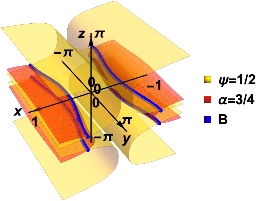
with the following  $(\unicode[STIX]{x1D713},\unicode[STIX]{x1D6FC})$ characteristics (see figure 1)
 $$\begin{eqnarray}\unicode[STIX]{x1D713}(X,Y,Z)=\sqrt{2\sinh (\sqrt{2}|X|)}\sin |Z|\end{eqnarray}$$
 $$\begin{eqnarray}\displaystyle & & \displaystyle \unicode[STIX]{x1D6FC}(X,Y,Z)=\unicode[STIX]{x1D6FF}\sqrt{\sinh (\sqrt{2}|X|)}\cos Y+\unicode[STIX]{x1D70E}_{z}\int _{|X_{0}|}^{|X|}{\displaystyle \frac{\text{d}X^{\prime }}{\sqrt{2\sinh (\sqrt{2}X^{\prime })-\unicode[STIX]{x1D713}^{2}}}},\nonumber\\ \displaystyle & & \displaystyle \quad \text{where,}~\unicode[STIX]{x1D70E}_{Z}=\text{sign}(\cos Z),X_{0}={\displaystyle \frac{1}{\sqrt{2}}}\sinh ^{-1}\left(\frac{\unicode[STIX]{x1D713}^{2}}{2}\right).\end{eqnarray}$$
 $\unicode[STIX]{x1D713}$ defined above is a single-valued function, whereas the function
 $\unicode[STIX]{x1D6FC}$ is not because of the second term in (3.3b). Note that, instead of
 $(\unicode[STIX]{x1D713},\unicode[STIX]{x1D6FC})$ we can also choose any functions of
 $(\unicode[STIX]{x1D713},\unicode[STIX]{x1D6FC})$, for example,
 $(\hat{\unicode[STIX]{x1D713}}=\unicode[STIX]{x1D713}^{2}/2,\hat{\unicode[STIX]{x1D6FC}}=\unicode[STIX]{x1D6FC}/\unicode[STIX]{x1D713})$ as the Clebsch coordinates.


The components of the magnetic field are
 $$\begin{eqnarray}\displaystyle & \displaystyle B_{X}=\sqrt{2}\unicode[STIX]{x1D6FF}\sin Y\cos Z\sinh \sqrt{2}X. & \displaystyle\end{eqnarray}$$
 $$\begin{eqnarray}\displaystyle & \displaystyle B_{Y}=1+\unicode[STIX]{x1D6FF}\cos Y\cos Z\cosh \sqrt{2}X. & \displaystyle\end{eqnarray}$$
 $$\begin{eqnarray}\displaystyle & \displaystyle B_{Z}=-\unicode[STIX]{x1D6FF}\sin Y\sin Z\cosh \sqrt{2}X. & \displaystyle\end{eqnarray}$$
 $\unicode[STIX]{x1D6FF}$ as a convenient expansion parameter in this work. To lowest order the magnetic field is
 $$\begin{eqnarray}B_{X}^{(0)}=0,\quad B_{Y}^{(0)}=1,\quad B_{Z}^{(0)}=0.\end{eqnarray}$$
The above equations show that the lowest-order magnetic field is of uniform strength  $(B^{(0)}=|\boldsymbol{B}^{(0)}|=1)$ and is purely in the
 $Y$ (toroidal) direction.
To describe the motion of the charged particles, we shall need to parametrize the magnetic field lines. Since the particles follow the magnetic field lines to the lowest order in the gyroradius, the coordinates used to describe the field lines will also determine the lowest-order particle trajectories. The equations describing the magnetic field lines are given by
 $$\begin{eqnarray}\displaystyle \frac{\text{d}X}{B_{X}}=\frac{\text{d}Y}{B_{Y}}=\frac{\text{d}Z}{B_{Z}}. & & \displaystyle\end{eqnarray}$$
Therefore,
 $$\begin{eqnarray}\displaystyle & \displaystyle \frac{\text{d}X}{\text{d}Y}=\frac{B_{X}}{B_{Y}}=\frac{\sqrt{2}\unicode[STIX]{x1D6FF}\sin Y\cos Z\sinh \sqrt{2}X}{1+\unicode[STIX]{x1D6FF}\cos Y\cos Z\cosh \sqrt{2}X} & \displaystyle\end{eqnarray}$$
 $$\begin{eqnarray}\displaystyle & \displaystyle \frac{\text{d}Z}{\text{d}Y}=\frac{B_{Z}}{B_{Y}}=\frac{-\unicode[STIX]{x1D6FF}\sin Y\sin Z\cosh \sqrt{2}X}{1+\unicode[STIX]{x1D6FF}\cos Y\cos Z\cosh \sqrt{2}X}. & \displaystyle\end{eqnarray}$$
 $$\begin{eqnarray}x=\sqrt{2}X,\quad y=Y,\quad z=Z,\quad \unicode[STIX]{x1D702}=\cos Y,\end{eqnarray}$$
and rewrite (3.7) as
 $$\begin{eqnarray}\displaystyle & \displaystyle \frac{\text{d}x}{\text{d}\unicode[STIX]{x1D702}}=\frac{-2\unicode[STIX]{x1D6FF}\cos z\sinh x}{1+\unicode[STIX]{x1D6FF}\unicode[STIX]{x1D702}\cos z\cosh x} & \displaystyle\end{eqnarray}$$
 $$\begin{eqnarray}\displaystyle & \displaystyle \frac{\text{d}z}{\text{d}\unicode[STIX]{x1D702}}=\frac{\unicode[STIX]{x1D6FF}\sin z\cosh x}{1+\unicode[STIX]{x1D6FF}\unicode[STIX]{x1D702}\cos z\cosh x}. & \displaystyle\end{eqnarray}$$
 $\unicode[STIX]{x1D6FF}$ will now be constructed. From the structure of (3.9) we find that
 $x$ and
 $z$ can be expanded in powers of
 $\unicode[STIX]{x1D6FF}$ as follows
 $$\begin{eqnarray}\left.\begin{array}{@{}c@{}}\displaystyle x=x_{0}+\unicode[STIX]{x1D6FF}x_{1}\unicode[STIX]{x1D702}+\unicode[STIX]{x1D6FF}^{2}x_{2}\unicode[STIX]{x1D702}^{2}+\cdots =\sum _{n}x_{n}\unicode[STIX]{x1D6FF}^{n}\unicode[STIX]{x1D702}^{n}\\ \displaystyle z=z_{0}+\unicode[STIX]{x1D6FF}z_{1}\unicode[STIX]{x1D702}+\unicode[STIX]{x1D6FF}^{2}z_{2}\unicode[STIX]{x1D702}^{2}+\cdots =\sum _{n}z_{n}\unicode[STIX]{x1D6FF}^{n}\unicode[STIX]{x1D702}^{n},\end{array}\right\}\end{eqnarray}$$
and substituting in (3.9) we obtain
 $$\begin{eqnarray}\left.\begin{array}{@{}c@{}}\displaystyle \frac{\text{d}x_{0}}{\text{d}\unicode[STIX]{x1D702}}+\unicode[STIX]{x1D6FF}\frac{\text{d}x_{1}}{\text{d}\unicode[STIX]{x1D702}}+O(\unicode[STIX]{x1D6FF}^{2})=-2\unicode[STIX]{x1D6FF}\sinh x_{0}+O(\unicode[STIX]{x1D6FF}^{2})\\ \displaystyle \frac{\text{d}z_{0}}{\text{d}\unicode[STIX]{x1D702}}+\unicode[STIX]{x1D6FF}\frac{\text{d}z_{1}}{\text{d}\unicode[STIX]{x1D702}}+O(\unicode[STIX]{x1D6FF}^{2})=\unicode[STIX]{x1D6FF}\cosh x\sin z_{0}+O(\unicode[STIX]{x1D6FF}^{2}).\end{array}\right\}\end{eqnarray}$$
Using (3.11) we determine  $x^{(n)}$ and
 $z^{(n)}$ order by order. In particular,
 $$\begin{eqnarray}\frac{\text{d}x_{0}}{\text{d}\unicode[STIX]{x1D702}}=0,\quad \frac{\text{d}z_{0}}{\text{d}\unicode[STIX]{x1D702}}=0,\end{eqnarray}$$
which shows that both  $x_{0}$ and
 $z_{0}$ must be constants. This is expected since the lowest-order magnetic field (3.5a–c) is purely in the
 $Y$ (toroidal) direction. The rest of
 $(x^{(n)},z^{(n)})$ are also obtained as functions of
 $(x_{0},z_{0})$.
The quantity  $q=\oint \text{d}l/B$ for this magnetic field (Weitzner & Sengupta Reference Weitzner and Sengupta2020), obtained as a function of
 $(x_{0},z_{0})$ is
 $$\begin{eqnarray}\frac{q}{2\unicode[STIX]{x03C0}}=1+\frac{1}{2}\cos ^{2}z_{0}\cosh ^{2}x_{0}\unicode[STIX]{x1D6FF}^{2}+O(\unicode[STIX]{x1D6FF}^{4}).\end{eqnarray}$$
3.2 Evaluation of the omnigeneity constraint
The equation for  $J_{\Vert }$ can be rewritten as
 $$\begin{eqnarray}\displaystyle J_{\Vert }=\oint v_{\Vert }\,\text{d}\ell =\oint v_{\Vert }\frac{\text{d}y}{B_{y}}. & & \displaystyle\end{eqnarray}$$
Since the lowest order  $B$ is 1, the above expression is approximately equivalent to
 $$\begin{eqnarray}\displaystyle J_{\Vert }\approx \oint v_{\Vert }\,\text{d}y=\oint \unicode[STIX]{x1D70E}\sqrt{2({\mathcal{E}}-\unicode[STIX]{x1D707}B)}\,\text{d}y. & & \displaystyle\end{eqnarray}$$
To evaluate  $J_{\Vert }$, we expand
 $B$ as follows
 $$\begin{eqnarray}B=\sqrt{B_{X}^{2}+B_{Y}^{2}+B_{Z}^{2}}=1+\unicode[STIX]{x1D6FF}\cos y\cos z_{0}\cosh x_{0}+O(\unicode[STIX]{x1D6FF}^{2}).\end{eqnarray}$$
Therefore,
 $$\begin{eqnarray}\left.\begin{array}{@{}c@{}}B=1+\unicode[STIX]{x1D6FF}B_{1}+O(\unicode[STIX]{x1D6FF}^{2}),\\ \text{where},\unicode[STIX]{x1D6FF}B_{1}=\unicode[STIX]{x1D6FF}_{0}\cos y\quad \text{and}\quad \unicode[STIX]{x1D6FF}_{0}=\unicode[STIX]{x1D6FF}\cosh x_{0}\cos z_{0}.\end{array}\right\}\end{eqnarray}$$
Since  $B$ is sinusoidal in
 $y$ to this order,
 $J_{\Vert }$ is identical to the action coordinates of a simple pendulum (Brizard Reference Brizard2011). We present the details of the calculation in appendix B.
We find that the lowest order  $J_{\Vert }$ for both trapped and circulating particles are functions of only
 $|\unicode[STIX]{x1D6FF}_{0}|$. From (3.13) we find that,
 $$\begin{eqnarray}\unicode[STIX]{x1D6FF}_{0}=\unicode[STIX]{x1D6FF}_{0}(q)\approx \sqrt{2}\sqrt{\frac{q}{2\unicode[STIX]{x03C0}}-1}.\end{eqnarray}$$
Hence,  $J_{\Vert }=J_{\Vert }(q)$ to lowest order. Since
 $q=q(\unicode[STIX]{x1D713},\unicode[STIX]{x1D6FC})$,
 $J_{\Vert }=J_{\Vert }(\unicode[STIX]{x1D713},\unicode[STIX]{x1D6FC})$ for both trapped and circulating particles. This shows that the closed field-line omnigeneity condition (2.28) is satisfied but not the omnigeneity condition (2.22) for field lines with flux surfaces.
3.3 Evaluation of the QS constraint
We have seen that the closed field-line omnigeneity condition is satisfied to lowest order. We now present the calculation of the QS constraints (2.29) to the lowest non-trivial order. We begin with the QS condition (2.23). We note from (3.4), (3.8) and (3.17) that
 $$\begin{eqnarray}\left.\begin{array}{@{}c@{}}\displaystyle \boldsymbol{B}\boldsymbol{\cdot }\unicode[STIX]{x1D735}=\frac{\unicode[STIX]{x2202}}{\unicode[STIX]{x2202}y}+\unicode[STIX]{x1D6FF}\left(\cos y\cos z\cosh x\frac{\unicode[STIX]{x2202}}{\unicode[STIX]{x2202}y}+2\sin y\left(\cos z\sinh x\frac{\unicode[STIX]{x2202}}{\unicode[STIX]{x2202}x}-\sin z\cosh x\frac{\unicode[STIX]{x2202}}{\unicode[STIX]{x2202}z}\right)\right)\\ \displaystyle \boldsymbol{B}\boldsymbol{\cdot }\unicode[STIX]{x1D735}B=\unicode[STIX]{x1D6FF}\frac{\unicode[STIX]{x2202}B_{1}}{\unicode[STIX]{x2202}y}+O(\unicode[STIX]{x1D6FF}^{2}),\quad \boldsymbol{B}\times \unicode[STIX]{x1D735}B=\unicode[STIX]{x1D6FF}\unicode[STIX]{x1D735}y\times \unicode[STIX]{x1D735}B_{1}+O(\unicode[STIX]{x1D6FF}^{2}).\end{array}\right\}\end{eqnarray}$$
From (3.3a) and (3.19) it follows that
 $$\begin{eqnarray}{\mathcal{F}}=\frac{\boldsymbol{B}\boldsymbol{\cdot }\unicode[STIX]{x1D735}\unicode[STIX]{x1D713}\times \unicode[STIX]{x1D735}B}{\boldsymbol{B}\boldsymbol{\cdot }\unicode[STIX]{x1D735}B}=\cot y\frac{\cosh x\cos z(2\tanh ^{2}x+\tan ^{2}z)}{\sqrt{\sinh x}}+O(\unicode[STIX]{x1D6FF}).\end{eqnarray}$$
The factor of  $\cot y$ implies that
 $\boldsymbol{B}\boldsymbol{\cdot }\unicode[STIX]{x1D735}{\mathcal{F}}\neq 0$. Hence the QS condition (2.23) is not satisfied.
However, the QS condition for closed field lines (2.29) is satisfied since
 $$\begin{eqnarray}\frac{{\mathcal{G}}}{\unicode[STIX]{x1D6FF}^{2}}=\frac{\boldsymbol{B}\boldsymbol{\cdot }\unicode[STIX]{x1D735}(q/\unicode[STIX]{x1D6FF}^{2})\times \unicode[STIX]{x1D735}B}{\boldsymbol{B}\boldsymbol{\cdot }\unicode[STIX]{x1D735}B}=\frac{\unicode[STIX]{x1D735}y\times \unicode[STIX]{x1D735}(q/\unicode[STIX]{x1D6FF}^{2})\boldsymbol{\cdot }\unicode[STIX]{x1D735}(\unicode[STIX]{x1D6FF}_{0}(q)\cos y)}{\unicode[STIX]{x2202}_{y}(\unicode[STIX]{x1D6FF}_{0}(q)\cos y)}+O(\unicode[STIX]{x1D6FF})=O(\unicode[STIX]{x1D6FF}).\end{eqnarray}$$
The division of  ${\mathcal{G}}$ by
 $\unicode[STIX]{x1D6FF}^{2}$ was done because
 $\unicode[STIX]{x1D735}q$ is of
 $O(\unicode[STIX]{x1D6FF}^{2})$. The lowest-order term in (3.21) vanishes, showing that the closed field-line QS condition is indeed satisfied to lowest order. Comparing (3.20) and (3.21), we see that the former is not QS while the latter is. It is to be noted that
 $\unicode[STIX]{x2202}_{\unicode[STIX]{x1D6FC}}q(\unicode[STIX]{x1D713},\unicode[STIX]{x1D6FC})\neq 0$ and hence
 $\unicode[STIX]{x1D713}$ and
 $q$ surfaces do not overlap.
QS can also be inferred from the expression for the field strength,
 $$\begin{eqnarray}B=1+\cos y\;\unicode[STIX]{x1D6FF}_{0}(q)+O(\unicode[STIX]{x1D6FF}^{2}).\end{eqnarray}$$
To first order,  $B$ depends only on one angle,
 $y$, when
 $q$ is used as a coordinate. Hence,
 $B$ is QS. We present a more detailed description of the QS calculation in appendix C.
3.4 Comparison of drift,  $\unicode[STIX]{x1D713}$ and $q$ surfaces


The drift surface of a charged particle obtained after averaging out the gyromotion and the bounce motion is a surface on which  $J_{\Vert }$ is constant (Gardner Reference Gardner1959). We shall now compare the drift surfaces with the constant
 $\unicode[STIX]{x1D713}$ and
 $q$ surfaces.
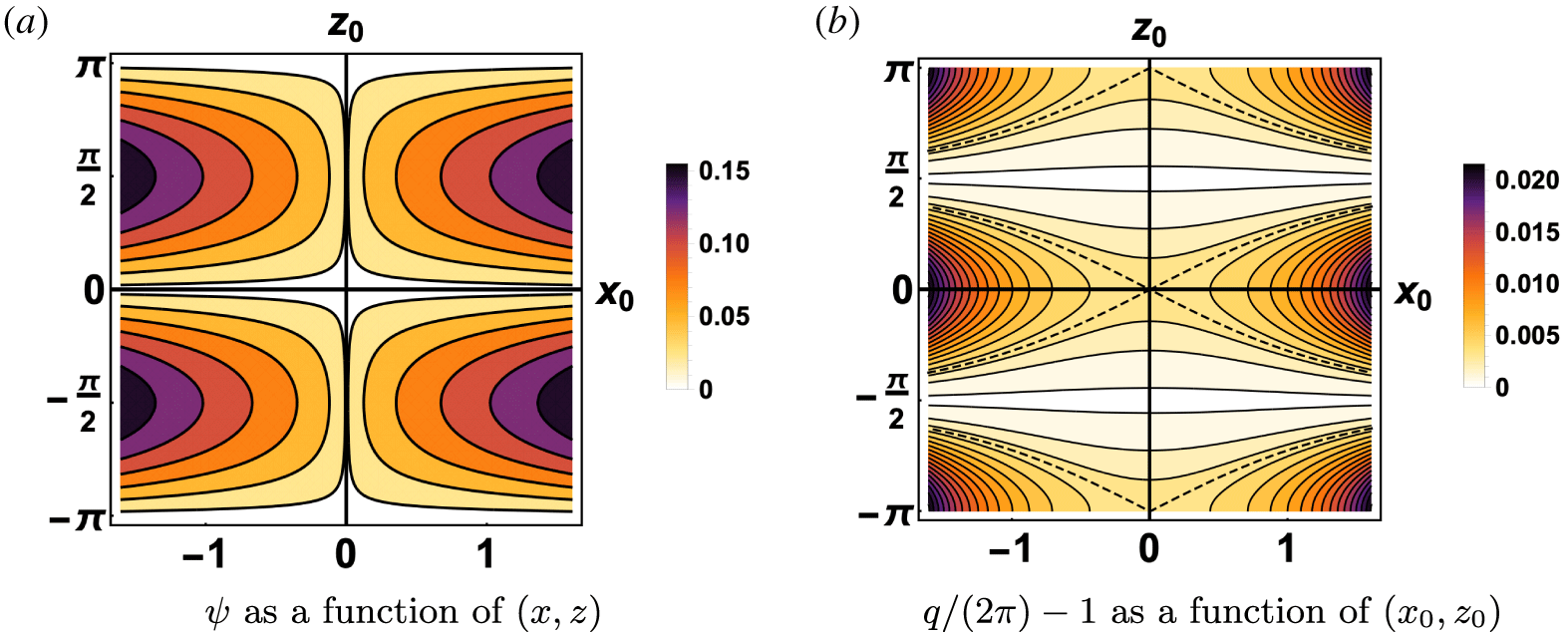
Figure 2 shows the constant  $\unicode[STIX]{x1D713}$ and
 $q$ contours. The contours of
 $q$ and
 $\unicode[STIX]{x1D713}$ do not coincide since
 $q=q(\unicode[STIX]{x1D713},\unicode[STIX]{x1D6FC})$. From the contours of the constant
 $\unicode[STIX]{x1D713}$ surfaces in figure 2(a) and (3.4), we see that the magnetic field has X-points at
 $(x=0,z=0)$ and
 $(x=0,z=\pm \unicode[STIX]{x03C0})$, where
 $B_{X}=B_{Z}=0$ but
 $B_{Y}\neq 0$. In a topological torus,
 $z=-\unicode[STIX]{x03C0}$ and
 $z=\unicode[STIX]{x03C0}$ are identified. Hence, there are only two X-points. The difference between
 $(x_{0},z_{0})$ and
 $(x,z)$ can be ignored for the lowest-order description that we are interested in, but must be taken into account for higher orders.
Contours of  $\unicode[STIX]{x1D713}$ and
 $q$ for
 $\unicode[STIX]{x1D6FF}=0.08$. The dotted lines in figure 2(b) is the separatrix
 $\cos z_{0}\cosh x_{0}=\pm 1$.

Drift surfaces (brown shades) of trapped particles superposed on  $q$ surfaces for
 $\unicode[STIX]{x1D716}=0.08$.

Drift surfaces (brown shades) of trapped particles superposed on  $\unicode[STIX]{x1D713}$ surfaces for
 $\unicode[STIX]{x1D716}=0.08$.

We have shown in § 3.2 and appendix B that  $J_{\Vert }$ and
 $q$ surfaces coincide to lowest order. In figure 3 we superpose the contours of constant
 $J_{\Vert }$ for trapped particles on top of contours of constant
 $q$. Figures 3(a) and 3(b) show the drift surfaces of particles trapped near
 $z_{0}=0$ and
 $z=\pm \unicode[STIX]{x03C0}$. In figure 4 we compare the trapped particle
 $J_{\Vert }$ with
 $\unicode[STIX]{x1D713}$ surfaces. It is clear that the particles will drift on a constant
 $q$ surfaces and not constant
 $\unicode[STIX]{x1D713}$ surfaces. If
 $q$ surfaces are closed, then all the particles will be confined. To the order of accuracy considered here,
 $q$ surfaces are not closed. However, obtaining closed
 $q$ surfaces is possible, as shown in Weitzner & Sengupta (Reference Weitzner and Sengupta2020).
We, therefore, conclude that the model magnetic field (3.4), which was not optimized to satisfy any constraint, turns out to be QS and hence omnigeneous to lowest order in  $\unicode[STIX]{x1D6FF}$, provided the closed field-line criteria (2.28) and (2.29) are used. The drift surfaces coincide with the pressure and
 $q$ surfaces and not the
 $\unicode[STIX]{x1D713}$ surfaces. Also, the model magnetic field is approximately QS in a given volume. Neither omnigeneity nor QS holds if the regular expressions (2.22) and (2.24), which are valid for irrational rotational transform, are used.
4 Discussion
In this work, we have investigated the radial confinement of particles in a magnetic field that has zero magnetic shear and all closed lines. We formulated the radial localization of particles and the omnigeneity and quasisymmetry constraints in terms of the pressure surfaces and not the flux surfaces. Our definitions are physically motivated since any confined equilibria should have closed pressure surfaces, and a configuration where particles stay localized near such closed surfaces should be ideal. However, in closed field-line systems, the pressure is a function of  $q=\oint \text{d}l/B$, which is, in general, dependent on both the Clebsch variables. Hence, the standard formulation of omnigeneity and quasisymmetry based on irrational rotational transform must be modified to take closed field lines into account. A closed field-line configuration where pressure surfaces (constant
 $q$) and drift surfaces (constant
 $J_{\Vert }$) coincide, if it exists, can be shown to be interchange stable (BenDaniel Reference BenDaniel1965; Hastie et al. Reference Hastie, Taylor and Haas1967). Differences between rational and irrational rotational transform also show up in the adiabatic invariants for circulating and trapped particles (Grad Reference Grad1967; Burby et al. Reference Burby, Kallinikos and MacKay2019). For ergodic field lines with flux surfaces, the drift orbits of circulating particles are always radially localized, unlike closed field-line systems.
We have then discussed drift orbits in a model magnetic field with closed field lines obtained recently (Weitzner & Sengupta Reference Weitzner and Sengupta2020). Expanding in a small parameter that measures the lack of symmetry of the magnetic fields, we show that the drift surfaces to lowest order are functions of  $q$. The model configuration is both omnigeneous and quasisymmetric according to the proposed constraints for closed field-line systems, but not any of these according to the general definitions valid for irrational rotational transform. Furthermore, we have shown that the system is approximately QS in a given volume. The analysis presented here suggests that optimization codes can easily miss out configurations where the drift surfaces coincide with the pressure surfaces in closed field-line configurations simply because the standard definitions of the omnigeneity and QS constraints are too restrictive.
The island divertors in low-shear stellarators have much longer connection lengths than tokamak divertors. Longer connection length implies that the cross-field transport is more important in the island divertor than in a tokamak divertor (Feng et al. Reference Feng, Sardei, Grigull, McCormick, Kisslinger and Reiter2006; Akerson et al. Reference Akerson, Bader, Hegna, Schmitz, Stephey, Anderson, Anderson and Likin2016). Since the drift surfaces characterize the collisionless cross-field motion of particles, our results show that, in closed field-line systems, the cross-field drift from both circulating particles and trapped particles can be significant. Also, in closed field-line systems, the function  $q$ can play a vital role in determining the drifts of the particles. In numerically optimizing stellarators for QS and fast-particle transport with low shear and near rational rotational transform configurations, the function
 $q$ could be relevant.
In the future, we shall consider extending the closed field omnigeneity and QS conditions to include the effects of small shear following Hastie et al. (Reference Hastie, Taylor and Haas1967) and Cary, Hedrick & Tolliver (Reference Cary, Hedrick and Tolliver1988). The class of exact vacuum solutions obtained in Weitzner & Sengupta (Reference Weitzner and Sengupta2020) is very large, and we can investigate which configuration, if any, can exactly or approximately satisfy omnigeneity or QS in a volume.
Acknowledgements
This work was done as part of the NYU Courant Institute Girls’ Science, Technology, Engineering and Mathematics (NYU GSTEM) Summer Program. E.E. would like to thank the GSTEM program for the opportunity; specifically, Catherine Tissot, for the work she put into it. In addition, we would like to thank H. Boland for being a supportive tutor. E.E. would like to thank everyone in the math department at Courant for the insightful conversations that were shared, especially J. McFadden, for all the books. The authors would also like to thank J. Perez and A. Cerfon for helpful suggestions.
This research was partly funded by the US DOE grant no. DEFG02-86ER53223.
Appendix A. Quasisymmetry and periodicity of $B$

Quasisymmetry can be formulated as a periodicity condition on  $B$ (Helander Reference Helander2014). For ergodic field lines with flux surfaces, the QS requirement is that the period is constant on the surface. Hence,
 $$\begin{eqnarray}B(\unicode[STIX]{x1D713},\unicode[STIX]{x1D6FC},l+L(\unicode[STIX]{x1D713}))=B(\unicode[STIX]{x1D713},\unicode[STIX]{x1D6FC},l).\end{eqnarray}$$
We now prove that the same property is true in a closed field-line system with the replacement of  $\unicode[STIX]{x1D713}$ by
 $q$. We start with the ideal MHD equilibrium conditions (2.10) with
 $(q,\overline{\unicode[STIX]{x1D6FC}})$ as the Clebsch potentials, and the QS condition (2.29)
 $$\begin{eqnarray}\displaystyle & \displaystyle \boldsymbol{B}=\unicode[STIX]{x1D735}q\times \unicode[STIX]{x1D735}\overline{\unicode[STIX]{x1D6FC}}=\frac{\unicode[STIX]{x1D735}q\times (\unicode[STIX]{x1D735}\unicode[STIX]{x1D6F7}\times \unicode[STIX]{x1D735}q)}{|\unicode[STIX]{x1D735}q|^{2}},\quad \unicode[STIX]{x1D735}q\times \unicode[STIX]{x1D735}\overline{\unicode[STIX]{x1D6FC}}\boldsymbol{\cdot }\unicode[STIX]{x1D735}\left(\frac{\unicode[STIX]{x1D735}q\boldsymbol{\cdot }\unicode[STIX]{x1D735}\unicode[STIX]{x1D6F7}}{|\unicode[STIX]{x1D735}q|^{2}}\right)=-p^{\prime }(q).\qquad & \displaystyle\end{eqnarray}$$
 $$\begin{eqnarray}\displaystyle & \displaystyle (\boldsymbol{B}\times \unicode[STIX]{x1D735}q-{\mathcal{G}}(q)\boldsymbol{B})\boldsymbol{\cdot }\unicode[STIX]{x1D735}B=0. & \displaystyle\end{eqnarray}$$
 $$\begin{eqnarray}\boldsymbol{B}\times \unicode[STIX]{x1D735}q=\unicode[STIX]{x1D735}\unicode[STIX]{x1D6F7}\times \unicode[STIX]{x1D735}q,\quad \boldsymbol{B}=\unicode[STIX]{x1D735}q\times \unicode[STIX]{x1D735}\overline{\unicode[STIX]{x1D6FC}},\end{eqnarray}$$
and  $(q,\overline{\unicode[STIX]{x1D6FC}},\unicode[STIX]{x1D6F7})$ coordinate system, we rewrite (A 2b) as
 $$\begin{eqnarray}\left(\frac{\unicode[STIX]{x2202}}{\unicode[STIX]{x2202}\overline{\unicode[STIX]{x1D6FC}}}-{\mathcal{G}}(q)\frac{\unicode[STIX]{x2202}}{\unicode[STIX]{x2202}\unicode[STIX]{x1D6F7}}\right)B=0.\end{eqnarray}$$
It follows from (A 4) that  $B$ must be of the form
 $$\begin{eqnarray}B(q,\overline{\unicode[STIX]{x1D6FC}},\unicode[STIX]{x1D6F7})={\mathcal{B}}(\unicode[STIX]{x1D6F7}+{\mathcal{G}}(q)\overline{\unicode[STIX]{x1D6FC}}).\end{eqnarray}$$
For fixed  $q$ and
 $\overline{\unicode[STIX]{x1D6FC}}$, the periodicity of
 $B$ is determined by the periods of
 $\unicode[STIX]{x1D6F7}$, which from (2.16) are functions of
 $q$, and therefore fixed on a constant
 $q$ surface. Hence, the QS periodicity requirement is satisfied. The exact same analysis is valid for ergodic field lines with
 $(q,\overline{\unicode[STIX]{x1D6FC}})$ replaced by
 $(\unicode[STIX]{x1D713},\unicode[STIX]{x1D6FC})$.
Appendix B. Details of the calculation of $J_{\Vert }$

We present here the details of the calculation of the drift surfaces for trapped and circulating particles. Trapped particles (TP) occupy the region where the magnetic field strength has a minimum. From (3.17), we see that the minima occur when
 $$\begin{eqnarray}\unicode[STIX]{x2202}_{y}^{2}B=-\unicode[STIX]{x1D6FF}_{0}(x_{0},z_{0})\cos y+O(\unicode[STIX]{x1D6FF}^{2})>0.\end{eqnarray}$$
Therefore, particles are trapped near  $y=\pm \unicode[STIX]{x03C0}$ for
 $\unicode[STIX]{x1D6FF}_{0}(x_{0},z_{0})>0$, and
 $y=0$ for
 $\unicode[STIX]{x1D6FF}_{0}(x_{0},z_{0})<0$. With the choice
 $\unicode[STIX]{x1D6FF}>0$, it follows from (3.17) that
 $$\begin{eqnarray}\unicode[STIX]{x1D6FF}_{0}(x_{0},z_{0})=\left\{\begin{array}{@{}ll@{}}\unicode[STIX]{x1D6FF}\cos z_{0}\cosh x_{0}<0,\quad & -\unicode[STIX]{x03C0}\leqslant z_{0}\leqslant -\unicode[STIX]{x03C0}/2\text{ and }+\unicode[STIX]{x03C0}/2\leqslant z_{0}\leqslant \unicode[STIX]{x03C0},\\ \unicode[STIX]{x1D6FF}\cos z_{0}\cosh x_{0}>0,\quad & -\unicode[STIX]{x03C0}/2\leqslant z_{0}\leqslant +\unicode[STIX]{x03C0}/2.\end{array}\right.\end{eqnarray}$$
We begin with the case where the particles are trapped near  $y=0$, i.e.
 $\unicode[STIX]{x1D6FF}_{0}<0$. To lowest non-trivial order,
 $J_{\Vert }$ is given by
 $$\begin{eqnarray}\displaystyle J_{\Vert }\approx \oint \unicode[STIX]{x1D70E}\sqrt{2({\mathcal{E}}-\unicode[STIX]{x1D707}(1-\unicode[STIX]{x1D6FF}_{r}\cos y))}\,\text{d}y, & & \displaystyle\end{eqnarray}$$
where
 $$\begin{eqnarray}\unicode[STIX]{x1D6FF}_{r}=-\unicode[STIX]{x1D6FF}_{0}=-\unicode[STIX]{x1D6FF}\cos z\cosh x\geqslant 0.\end{eqnarray}$$
For TP the  $J_{\Vert }$ integral is carried out between the bounce points
 $-y_{b}$ and
 $+y_{b}$. Taking into account that
 $\unicode[STIX]{x1D70E}$ can be
 $\pm 1$ for trapped particles,
 $$\begin{eqnarray}J_{\Vert }^{TP}=2\int _{-y_{b}}^{+y_{b}}\sqrt{2({\mathcal{E}}-\unicode[STIX]{x1D707}(1-\unicode[STIX]{x1D6FF}_{r}\cos y))}\,\text{d}y.\end{eqnarray}$$
At the endpoints,
 $$\begin{eqnarray}{\mathcal{E}}/\unicode[STIX]{x1D707}=B(y_{b})=(1-\unicode[STIX]{x1D6FF}_{r}\cos y_{b}).\end{eqnarray}$$
Solving for the bounce point we get,
 $$\begin{eqnarray}\sin ^{2}\frac{y_{b}}{2}=\frac{{\mathcal{E}}/\unicode[STIX]{x1D707}-(1-\unicode[STIX]{x1D6FF}_{r})}{2\unicode[STIX]{x1D6FF}_{r}},\end{eqnarray}$$
which implies that the trapped particles localized near  $y=0$, have
 ${\mathcal{E}}/\unicode[STIX]{x1D707}$ ratio bounded between
 $$\begin{eqnarray}\displaystyle 1-\unicode[STIX]{x1D6FF}_{r}\leqslant \frac{{\mathcal{E}}}{\unicode[STIX]{x1D707}}\leqslant 1+\unicode[STIX]{x1D6FF}_{r}. & & \displaystyle\end{eqnarray}$$
The  $J_{\Vert }$ integral takes the following form
 $$\begin{eqnarray}\displaystyle J_{\Vert }^{TP}=2\sqrt{\unicode[STIX]{x1D707}\unicode[STIX]{x1D6FF}_{r}}\int _{-y_{b}}^{y_{b}}\sqrt{\sin ^{2}\frac{y_{b}}{2}-\sin ^{2}\frac{y}{2}}\,\text{d}y. & & \displaystyle\end{eqnarray}$$
For deeply trapped particles  $\sin y\approx y$, therefore,
 $$\begin{eqnarray}\displaystyle J_{\Vert }^{TP}=2\unicode[STIX]{x03C0}\left(\frac{y_{b}}{2}\right)^{2}\sqrt{\unicode[STIX]{x1D707}\unicode[STIX]{x1D6FF}_{r}}\;. & & \displaystyle\end{eqnarray}$$
In general  $J_{\Vert }$ can be written in terms of elliptic integrals (Brizard Reference Brizard2011),
 $$\begin{eqnarray}\displaystyle J_{\Vert }^{TP}=8\sqrt{\unicode[STIX]{x1D707}\unicode[STIX]{x1D6FF}_{r}}(E(k^{2})-(1-k^{2})K(k^{2})),\quad k=\sin \frac{y_{b}}{2}. & & \displaystyle\end{eqnarray}$$
For particle trapped near  $y=\pm \unicode[STIX]{x03C0}$, we shift
 $y$ to
 $y^{\prime }=y\pm \unicode[STIX]{x03C0}$ such that
 $\cos y=-\cos y^{\prime }$. Also,
 $$\begin{eqnarray}\sin ^{2}\frac{y_{b}^{\prime }}{2}=\frac{{\mathcal{E}}/\unicode[STIX]{x1D707}-(1-\unicode[STIX]{x1D6FF}_{0})}{2\unicode[STIX]{x1D6FF}_{0}},\quad 1-\unicode[STIX]{x1D6FF}_{0}\leqslant \frac{{\mathcal{E}}}{\unicode[STIX]{x1D707}}\leqslant 1+\unicode[STIX]{x1D6FF}_{0}.\end{eqnarray}$$
Both of these cases can be represented by (B 11) with  $\unicode[STIX]{x1D6FF}_{r}$ replaced by
 $|\unicode[STIX]{x1D6FF}_{0}|$.
Similarly, for circulating particles (CP), carrying out the integration from  $0$ to
 $2\unicode[STIX]{x03C0}$, we obtain
 $$\begin{eqnarray}J_{\Vert }^{CP}=4\unicode[STIX]{x1D70E}\sqrt{\unicode[STIX]{x1D707}|\unicode[STIX]{x1D6FF}_{0}|}kE(1/k^{2}),\quad \text{where }k^{2}=\frac{{\mathcal{E}}/\unicode[STIX]{x1D707}-(1-|\unicode[STIX]{x1D6FF}_{0}|)}{2|\unicode[STIX]{x1D6FF}_{0}|}.\end{eqnarray}$$
Appendix C. Details of the QS calculation
The function  $q$ is a function of
 $(x_{0},z_{0})$, it is convenient to rewrite the QS condition (2.29) in terms of
 $(x_{0},z_{0})$. Along the field-line characteristics (3.9)
 $$\begin{eqnarray}x=\mathop{\sum }_{n=0}^{\infty }(\unicode[STIX]{x1D6FF}\unicode[STIX]{x1D702})^{n}x^{(n)}(x_{0},z_{0}),\quad y=\cos ^{-1}\unicode[STIX]{x1D702},\quad z=\mathop{\sum }_{n=0}^{\infty }(\unicode[STIX]{x1D6FF}\unicode[STIX]{x1D702})^{n}z^{(n)}(x_{0},z_{0}).\end{eqnarray}$$
Taking the gradient with respect to the  $(x,y,z)$ coordinate system we get
 $$\begin{eqnarray}\left(\begin{array}{@{}c@{}}\unicode[STIX]{x1D735}x\\ \unicode[STIX]{x1D735}y\\ \unicode[STIX]{x1D735}z\end{array}\right)=\left(\begin{array}{@{}ccc@{}}{\displaystyle \frac{\unicode[STIX]{x2202}x}{\unicode[STIX]{x2202}x_{0}}} & {\displaystyle \frac{\unicode[STIX]{x2202}x}{\unicode[STIX]{x2202}\unicode[STIX]{x1D702}}} & {\displaystyle \frac{\unicode[STIX]{x2202}x}{\unicode[STIX]{x2202}z_{0}}}\\ 0 & {\displaystyle \frac{\text{d}y}{\text{d}\unicode[STIX]{x1D702}}} & 0\\ {\displaystyle \frac{\unicode[STIX]{x2202}z}{\unicode[STIX]{x2202}x_{0}}} & {\displaystyle \frac{\unicode[STIX]{x2202}z}{\unicode[STIX]{x2202}\unicode[STIX]{x1D702}}} & {\displaystyle \frac{\unicode[STIX]{x2202}z}{\unicode[STIX]{x2202}z_{0}}}\end{array}\right)\left(\begin{array}{@{}c@{}}\unicode[STIX]{x1D735}x_{0}\\ \unicode[STIX]{x1D735}\unicode[STIX]{x1D702}\\ \unicode[STIX]{x1D735}z_{0}\end{array}\right),\end{eqnarray}$$
which can be inverted to obtain
 $$\begin{eqnarray}\left(\begin{array}{@{}c@{}}\unicode[STIX]{x1D735}x_{0}\\ \unicode[STIX]{x1D735}\unicode[STIX]{x1D702}\\ \unicode[STIX]{x1D735}z_{0}\end{array}\right)={\displaystyle \frac{1}{\{x,z\}_{(x_{0},z_{0})}}}\left(\begin{array}{@{}ccc@{}}{\displaystyle \frac{\unicode[STIX]{x2202}z}{\unicode[STIX]{x2202}z_{0}}} & {\displaystyle \frac{\text{d}\unicode[STIX]{x1D702}}{\text{d}y}}\{x,z\}_{(z_{0},\unicode[STIX]{x1D702})} & -{\displaystyle \frac{\unicode[STIX]{x2202}x}{\unicode[STIX]{x2202}z_{0}}}\\ 0 & {\displaystyle \frac{\text{d}\unicode[STIX]{x1D702}}{\text{d}y}} & 0\\ -{\displaystyle \frac{\unicode[STIX]{x2202}z}{\unicode[STIX]{x2202}x_{0}}} & {\displaystyle \frac{\text{d}\unicode[STIX]{x1D702}}{\text{d}y}}\{x,z\}_{(\unicode[STIX]{x1D702},x_{0})} & {\displaystyle \frac{\unicode[STIX]{x2202}x}{\unicode[STIX]{x2202}x_{0}}}\end{array}\right)\left(\begin{array}{@{}c@{}}\unicode[STIX]{x1D735}x\\ \unicode[STIX]{x1D735}y\\ \unicode[STIX]{x1D735}z\end{array}\right),\end{eqnarray}$$
where  $\{x,z\}_{(a,b)}$ denotes the Poisson bracket of
 $(x,z)$ with respect to
 $(a,b)$. It follows that
 $$\begin{eqnarray}\displaystyle \unicode[STIX]{x1D735}q(x_{0},z_{0}) & = & \displaystyle {\displaystyle \frac{1}{\{x,z\}_{(x_{0},z_{0})}}}\left(\{q,z\}_{(x_{0},z_{0})}\unicode[STIX]{x1D735}x+\{x,q\}_{(x_{0},z_{0})}\unicode[STIX]{x1D735}z\right.\nonumber\\ \displaystyle & & \displaystyle +\left.{\displaystyle \frac{\text{d}\unicode[STIX]{x1D702}}{\text{d}y}}\left({\displaystyle \frac{\unicode[STIX]{x2202}q}{\unicode[STIX]{x2202}x_{0}}}\{x,z\}_{(z_{0},\unicode[STIX]{x1D702})}+{\displaystyle \frac{\unicode[STIX]{x2202}q}{\unicode[STIX]{x2202}z_{0}}}\{x,z\}_{(\unicode[STIX]{x1D702},x_{0})}\right)\right)\unicode[STIX]{x1D735}y.\end{eqnarray}$$
Since  $q$ is of the form
 $q=2\unicode[STIX]{x03C0}+q^{(2)}\unicode[STIX]{x1D6FF}^{2}+O(\unicode[STIX]{x1D6FF}^{4})$ (3.13),
 $$\begin{eqnarray}\left.\begin{array}{@{}c@{}}\displaystyle \{x,z\}_{(x_{0},z_{0})}=1+\unicode[STIX]{x1D6FF}\unicode[STIX]{x1D702}\left({\displaystyle \frac{\unicode[STIX]{x2202}x_{1}}{\unicode[STIX]{x2202}x_{0}}}+{\displaystyle \frac{\unicode[STIX]{x2202}z_{1}}{\unicode[STIX]{x2202}z_{0}}}\right)+O(\unicode[STIX]{x1D6FF}^{2}),\\ \displaystyle \{x,z\}_{(z_{0},\unicode[STIX]{x1D702})}=-\unicode[STIX]{x1D6FF}x_{1}+O(\unicode[STIX]{x1D6FF}^{2}),\quad \{x,z\}_{(\unicode[STIX]{x1D702},x_{0})}=-\unicode[STIX]{x1D6FF}z_{1}+O(\unicode[STIX]{x1D6FF}^{2}),\\ \displaystyle \{q,z\}_{(x_{0},z_{0})}=\unicode[STIX]{x1D6FF}^{2}{\displaystyle \frac{\unicode[STIX]{x2202}q^{(2)}}{\unicode[STIX]{x2202}x_{0}}}++O(\unicode[STIX]{x1D6FF}^{3}),\quad \{x,q\}_{(x_{0},z_{0})}=\unicode[STIX]{x1D6FF}^{2}{\displaystyle \frac{\unicode[STIX]{x2202}q^{(2)}}{\unicode[STIX]{x2202}z_{0}}}+O(\unicode[STIX]{x1D6FF}^{3}).\end{array}\right\}\end{eqnarray}$$
Therefore,
 $$\begin{eqnarray}\left.\begin{array}{@{}c@{}}\displaystyle \unicode[STIX]{x1D735}(q/\unicode[STIX]{x1D6FF}^{2})=\left({\displaystyle \frac{\unicode[STIX]{x2202}q^{(2)}}{\unicode[STIX]{x2202}x_{0}}}\unicode[STIX]{x1D735}x+{\displaystyle \frac{\unicode[STIX]{x2202}q^{(2)}}{\unicode[STIX]{x2202}z_{0}}}\unicode[STIX]{x1D735}z\right)+O(\unicode[STIX]{x1D6FF})\\ \displaystyle \boldsymbol{B}\times \unicode[STIX]{x1D735}B\boldsymbol{\cdot }\unicode[STIX]{x1D735}(q/\unicode[STIX]{x1D6FF}^{2})=\unicode[STIX]{x1D6FF}\{q^{(2)},{B_{1}\}}_{(x_{0},z_{0})}+O(\unicode[STIX]{x1D6FF}).\end{array}\right\}\end{eqnarray}$$
From (3.17), (3.13) we get  $\unicode[STIX]{x1D6FF}B_{1}=\sqrt{q^{(2)}}$. Therefore,
 $$\begin{eqnarray}\boldsymbol{B}\times \unicode[STIX]{x1D735}B\boldsymbol{\cdot }\unicode[STIX]{x1D735}(q/\unicode[STIX]{x1D6FF}^{2})=O(\unicode[STIX]{x1D6FF}).\end{eqnarray}$$