1 Introduction
The entrainment of fluid across a sheared density interface is a canonical problem in fluid mechanics with direct application to the upper atmosphere, oceanic flow and estuaries. We examine a common environmental setting for this flow in which a dense fluid is situated within a depression and purged by a less dense overflow. This particular arrangement can be seen for example in valleys and urban street canyons (Kirkpatrick & Armfield Reference Kirkpatrick and Armfield2005; Chang, Constantinescu & Park Reference Chang, Constantinescu and Park2006; Fernando et al. Reference Fernando, Zajic, Di Sabatino, Dimitrova, Hedquist and Dallman2010; Baratian-Ghorghi & Kaye Reference Baratian-Ghorghi and Kaye2013) as well in estuaries and ocean trenches (Abraham Reference Abraham1988; Debler & Imberger Reference Debler and Imberger1996). In lowland Australian rivers this flow is produced by saline ground water intrusions in deep river pools. These pools are associated with high nutrient levels and low oxygen concentrations. This environmental issue can be managed by release of stored water upstream, which can purge the saline intrusions from the pools by turbulent entrainment. The relationship between the entrainment or purging rate and the cavity geometry and flow parameters is a critical issue.
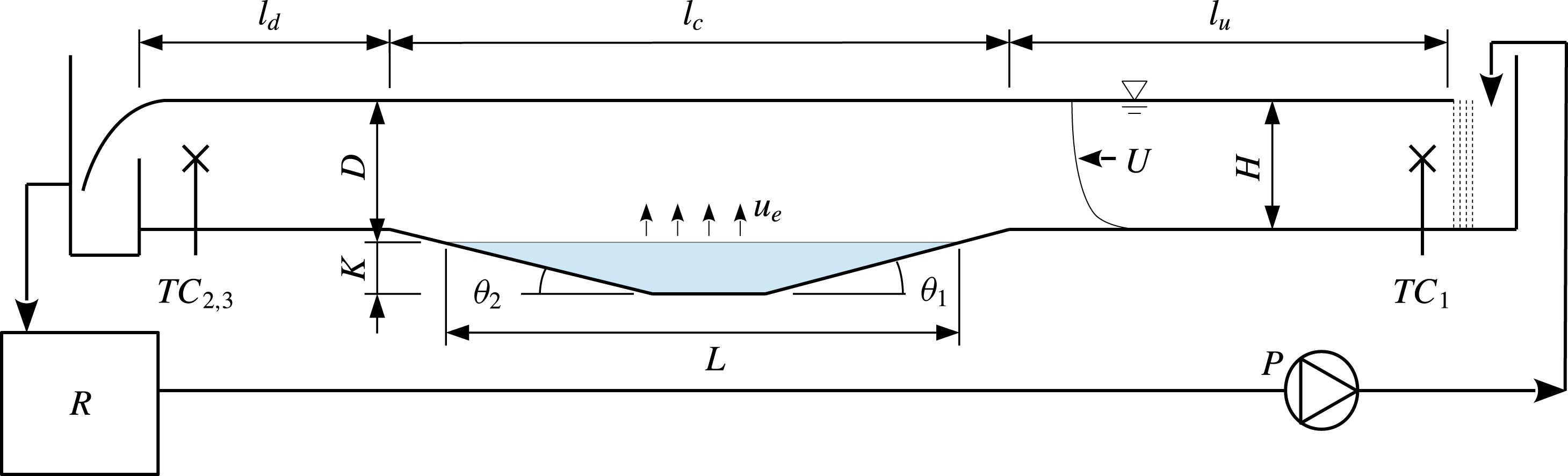
Schematic representation of the flow and experimental apparatus. Flow is from right to left and re-circulates via a reservoir.

A schematic representation of our laboratory model of this flow is given in figure 1. Fresh water flows from right to left through an open channel of depth
 $H$
at bulk velocity
 $U_{0}$
. A cavity containing more dense saline water at an initial depth
 $K_{0}$
and length
 $l_{c}$
, is located at the base of the channel. The saline fluid is entrained into the overflow with a characteristic entrainment velocity
 $u_{e}$
. In this model the cavity fluid is not replaced, so over time the cavity interface depth
 $K$
and interface length
 $L$
decrease while the depth of the mixed layer
 $D$
increases. The bulk velocity in the mixed layer
 $U_{b}$
is time varying within each experiment in response to
 $D$
varying, with
 $U_{b}=U_{0}H/D$
. The rate of this fluid exchange and its underlying mechanism are the subject of this investigation. In this setting the entrainment velocity
 $u_{e}$
is expected to contain a functional dependence
 $$\begin{eqnarray}u_{e}=f_{1}(\unicode[STIX]{x0394}b,\unicode[STIX]{x0394}U,D,L,K,H,\unicode[STIX]{x1D703}_{1},\unicode[STIX]{x1D703}_{2},\unicode[STIX]{x1D708},\unicode[STIX]{x1D705}),\end{eqnarray}$$
where the buoyancy difference
 $\unicode[STIX]{x0394}b=g\unicode[STIX]{x0394}\unicode[STIX]{x1D70C}/\unicode[STIX]{x1D70C}_{0}$
, where
 $\unicode[STIX]{x0394}\unicode[STIX]{x1D70C}=\unicode[STIX]{x1D70C}-\unicode[STIX]{x1D70C}_{0}$
, with
 $\unicode[STIX]{x1D70C}_{0}$
and
 $\unicode[STIX]{x1D70C}$
being the density of the cavity fluid and overflow fluid, respectively. The molecular diffusivity of the saline fluid is denoted by
 $\unicode[STIX]{x1D705}$
,
 $\unicode[STIX]{x1D708}$
is the kinematic viscosity and
 $\unicode[STIX]{x0394}U$
is the velocity jump across the interface. The cavity fluid is nearly quiescent in this flow so
 $\unicode[STIX]{x0394}U\sim U_{b}$
. The turbulent mixed layer depth
 $D$
and bulk velocity
 $U_{b}$
are then the natural choice of scales for this sheared interface problem as has been shown in other flow arrangements (Price Reference Price1979; Narimousa & Fernando Reference Narimousa and Fernando1987; Strang & Fernando Reference Strang and Fernando2001). The bulk Richardson number for this flow is
 $$\begin{eqnarray}Ri_{b}=\frac{g\unicode[STIX]{x0394}\unicode[STIX]{x1D70C}D}{\unicode[STIX]{x1D70C}_{0}U_{b}^{2}}.\end{eqnarray}$$
The non-dimensional entrainment rate
 $E=u_{e}/U_{b}$
is expected to contain the functional dependence
 $$\begin{eqnarray}E=f_{2}(Ri_{b},Re,Sc,A),\end{eqnarray}$$
where
 $Re=U_{b}D/\unicode[STIX]{x1D708}$
,
 $Sc=\unicode[STIX]{x1D708}/\unicode[STIX]{x1D705}$
and
 $A$
contains the relevant geometric properties
 $A=[L/D,L/H,D/H,\unicode[STIX]{x1D703}_{1},\unicode[STIX]{x1D703}_{2}]$
. The functional dependence on the cavity depth
 $K$
is seen through the ratio
 $D/H$
, as
 $(D+K)/H$
is a constant. In this study we consider flow with small values of
 $\unicode[STIX]{x1D703}_{1}$
and
 $\unicode[STIX]{x1D703}_{2}$
, with the goal of avoiding separation of the flow from the upstream entry slope. In this situation
 $\unicode[STIX]{x1D703}$
is expected to have minimal influence and is excluded from further consideration.
The dependence of the entrainment rate on the interface development length
 $L$
is unclear.
Previous studies of low-aspect-ratio cavities, where
 $l_{c}/K_{0}\simeq 1$
to 2 (Strang & Fernando Reference Strang and Fernando2004; Kirkpatrick & Armfield Reference Kirkpatrick and Armfield2005; Baratian-Ghorghi & Kaye Reference Baratian-Ghorghi and Kaye2013), have shown that the flow can be characterised by an interface entrainment mechanism coupled with a turbulent exchange mechanism between the turbulent overflow and the cavity interior. In this geometric range, the overflow separates from the leading edge of the cavity, and circulation within the cavity is significant (Kirkpatrick & Armfield Reference Kirkpatrick and Armfield2005).
Debler & Armfield (Reference Debler and Armfield1997) performed experiments at larger aspect ratios up to
 $l_{c}/K_{0}=16.7$
and also varied cavity entry and exit angles to develop a scaling for the purging rate which accounts for interface height. Entrainment rate measurements were sensitive to cavity geometry, and dye visualisation indicated this was associated with flow separation at the cavity corners. Chu & Baddour (Reference Chu and Baddour1984) used laboratory experiments to examine a cavity-like flow where a planar surface jet was issued from a square-edged outlet flush with a density interface. The authors examined the development of the surface jet and showed that the flow initially expands as a planar wall jet where the velocity profile is approximately self-similar. The expansion rate was shown to be close to that of a non-buoyant wall jet. We refer to this as region 1. Downstream the expansion of the jet eventually ceased and a parallel flow was observed where the mixing layer thickness was observed to grow more slowly. We refer to this as region 2. Kirkpatrick, Armfield & Williamson (Reference Kirkpatrick, Armfield and Williamson2012) showed, using large eddy simulation (LES) and the experimental results of Debler & Armfield (Reference Debler and Armfield1997), that the entrainment behaviour in the cavity flow can be similarly delineated between these two distinct regions. The mixed layer initially expands over the cavity with the length and velocity scales of a planar surface jet. The entrainment in region 1 has the behaviour
 $u_{e}/U_{0}\sim Ri^{-1}$
. Further along the cavity the flow has the characteristics of a planar mixing layer (region 2) with local scales
 $D$
and
 $U_{b}$
, and the authors found
 $u_{e}/U_{b}\sim Ri_{b}^{n}$
where
 $n\simeq -1$
. The authors found improved correlation with experimental data sets using this two-region scaling relationship. Experimental verification of this model has been incomplete, however, as previous cavity flow experiments and simulations have contained a high proportion of the region 1 mode of entrainment owing to the small aspect ratio.
The dynamics of region 2 mode entrainment, being a sheared two-layer stratified flow, have been examined in other laboratory settings. Lofquist (Reference Lofquist1960) examined flow in a straight channel whereby a submerged saline wall jet introduced beneath otherwise quiescent fresh fluid produced two-layer shear flow. Sullivan & List (Reference Sullivan and List1994) generated a sheared two-layer flow using splitter plates to separate two opposing flow streams of saline and fresh water in a straight open channel. In both studies quasi-steady conditions were developed. Kato & Phillips (Reference Kato and Phillips1969) produced stable linearly stratified shear flow in a re-circulating annulus driven by constant surface shear. A similar approach was later used by Kantha, Phillips & Azad (Reference Kantha, Phillips and Azad1977) and Deardorff & Willis (Reference Deardorff and Willis1982) to attain two-layer stratified flow. Narimousa, Long & Kitaigorodskii (Reference Narimousa, Long and Kitaigorodskii1986) and Narimousa & Fernando (Reference Narimousa and Fernando1987) used a re-circulating Odell–Kovasznay water channel to produce a two-layer stratified flow with the mixed layer being driven by a disc pump. The entrainment rate measurements obtained from this apparatus had significantly reduced scatter compared with earlier studies, enabling Strang & Fernando (Reference Strang and Fernando2001) to present a regime map for interface behaviour across a Richardson range of
 $Ri_{b}\simeq 1$
to 20. The authors correlated the entrainment with the bulk parameters
 $U_{b}$
and
 $D$
to obtain the scaling
 $u_{e}/U_{b}\sim Ri_{b}^{-n}$
. The exponent
 $n$
was found to vary between two flow regimes, with
 $n=-2.63$
over
 $1.5<Ri_{b}<5$
and
 $n=-1.3$
over
 $5<Ri_{b}<20$
. The authors showed that the entrainment process is comprised of interfacial mixing across the density interface into an intermediate layer coupled with turbulent transport from the intermediate layer into the turbulent mixed layer, in line with earlier observations of Narimousa & Fernando (Reference Narimousa and Fernando1987) and Sullivan & List (Reference Sullivan and List1994). Using observations of the temporal variation in interface structure and the turbulent kinetic energy budget, Strang & Fernando (Reference Strang and Fernando2001) were able to show for
 $Ri_{b}<5$
the entrainment rate is limited by turbulent mixing in the mixed layer while for
 $Ri_{b}>5$
the entrainment is limited by interfacial mixing leading to a relatively thin interfacial layer. This demarcation corresponds to the destabilisation at the interface, where for
 $Ri_{b}<5$
the interface was characterised by Kelvin–Helmholtz (K–H) waves, while above
 $Ri_{b}=5.8$
symmetric Holmboe waves were the dominant characteristic. Direct numerical simulation studies have shown the contrasting mixing of these instabilities across their development. The turbulence generated in the breakdown of Holmboe waves can be significantly lower that of K–H waves at low Reynolds numbers (Smyth, Carpenter & Lawrence Reference Smyth, Carpenter and Lawrence2007; Salehipour, Caulfield & Peltier Reference Salehipour, Caulfield and Peltier2016).
The scatter in previous studies makes the generality of the entrainment rate scaling unclear. For example, the entrainment rates measurement by Deardorff & Willis (Reference Deardorff and Willis1982) are approximately an order of magnitude smaller than those of Strang & Fernando (Reference Strang and Fernando2001). The interfacial mixing is a product of both the stability of the interface and the disturbance applied by the flow. The local effect of sidewalls, lateral circulation, surface and bottom wall shear, and the transport of turbulence from any upstream disturbances, such as a boundary layer or pumps, are all expected to modify the turbulent mixing at the interface and transport within the mixed layer, leading to variations among different laboratory configurations. Further understanding of these influences is critical. Our motivation is to obtain the scaling for region 2 mode entrainment in the cavity setting, and also to provide an additional data set for two-layer stratified flow more generally, so that these influences may be further quantified. The present cavity flow configuration differs from the studies of Deardorff & Willis (Reference Deardorff and Willis1982) and Strang & Fernando (Reference Strang and Fernando2001) in that the flow is a spatially developing stratified mixing layer rather than a temporally developing flow. A key feature of this configuration is that, as the interface fluid is advected downstream, it is replaced by saline fluid within the cavity at density
 $\unicode[STIX]{x1D70C}_{0}$
. This behaviour is seen in the numerical simulations of Kirkpatrick et al. (Reference Kirkpatrick, Armfield and Williamson2012). In this way the upstream limit of the mixing layer is continually renewed during the flow, thereby ensuring that at its origin the mixing layer remains sharp for all Richardson numbers.
A new laboratory rig has been designed to obtain a sheared two-layer stratified flow within the cavity flow setting, and to allow for a variable interface development length. This apparatus is described in § 2. We have performed two types of experiments. We initially report on cavity-averaged ‘bulk’ entrainment measurements in § 3 and test the functional dependence of the scaling for the entrainment rate. In § 4 we report on further measurements of local interface thickness and shear layer thickness and observations of the interface structure.
2 Laboratory rig
Our laboratory rig, illustrated in figure 1, has a channel width
 $B=0.50~\text{m}$
, an upstream development length of
 $l_{u}=2.5~\text{m}$
, downstream length
 $l_{d}=1.4~\text{m}$
. The channel depth at the entrance to the cavity, the cavity depth and overflow height are constant at
 $K_{0}=D_{0}=H=0.1~\text{m}$
. The cavity entry and exit angles are
 $\unicode[STIX]{x1D703}_{1}=6.2^{\circ }$
and
 $\unicode[STIX]{x1D703}_{2}=8.0^{\circ }$
, respectively. The slope is sufficiently small such that in all experiments the overflow remains attached to the cavity entry slope and there is no flow re-circulation behind the exit slope. Cavity lengths of
 $l_{c}=1.6~\text{m}$
and
 $l_{c}=2.1~\text{m}$
were tested. The variation is achieved by inserting extensions to the upstream channel into the base of the cavity. Additionally, within each experiment, the interface depth
 $D$
increases as entrainment erodes the interface and the length of the interface
 $L$
, then decreases due to the slope of the cavity upstream and downstream walls. In this way, although only two initial values of
 $l_{c}$
are used, the total experimental range of
 $L/D$
is large.
During an experiment, water is circulated through the channel via a
 $0.9~\text{m}^{3}$
storage reservoir denoted
 $R$
in figure 1. The water is pumped from the reservoir to the plenum box at the start of the channel, after which it flows through flow straighteners and then along the channel, over the cavity to an overflow weir at the end, and returns to the storage reservoir. The reservoir level is maintained at
 $0.55~\text{m}^{3}$
capacity and is stirred continuously by submersible pumps with a total capacity of
 $800~\text{l}~\min ^{-1}$
, to maintain a homogeneous but time-varying reservoir salinity.
The experimental preparation requires the channel and cavity to be initially filled with fresh water. Additional saline water is then introduced into the cavity base, displacing the fresh water, so a sharp stable two-layer saline stratification is achieved. The cavity is filled with saline fluid to
 $K=K_{0}=0.1~\text{m}$
. To commence an experiment, the flow is initiated by turning on the fresh water pump. The initial start-up of the flow sets up a wave in the cavity interface and ‘splashes’ out a volume of cavity fluid (Debler & Armfield Reference Debler and Armfield1997; Gillam, Armfield & Kirkpatrick Reference Gillam, Armfield and Kirkpatrick2009). The initial splash and cavity seiche is reduced by initiating the flow with a 120 second ramped start-up. Data are only retained once the transient start-up effects have dissipated, by which time the interface level has decreased and has a length that is less than
 $l_{c}$
. The experiments were stopped before the interface depth reduced to
 $K=0.018~\text{m}$
to limit interaction between the density interface and the base of the cavity. For
 $l_{c}=1.6~\text{m}$
this limit corresponds to
 $L/D=16$
in figure 2.
3 Entrainment measurements
Experiments were initially performed with the goal of understanding the functional dependence of the bulk entrainment on the following parameters:
 $$\begin{eqnarray}E\simeq f_{3}\left(Ri_{b},Re,\frac{L}{D},\frac{D}{H}\right).\end{eqnarray}$$
Most of the experiments were performed with a channel flow velocity of
 $U_{0}=0.113~\text{m}~\text{s}^{-1}$
, giving a Reynolds number of
 $Re=11\,300$
. Additional runs were performed at
 $0.071~\text{m}~\text{s}^{-1}$
and
 $0.151~\text{m}~\text{s}^{-1}$
, giving
 $Re=7100$
and
 $Re=15\,100$
, respectively. The Froude number for the free surface channel flow is
 $Fr=0.07$
to 0.15, which is well within the subcritical flow regime. The density difference between the cavity fluid
 $\unicode[STIX]{x1D70C}_{0}$
and the mixed layer
 $\unicode[STIX]{x1D70C}$
was obtained by varying the cavity fluid salinity (
 $\unicode[STIX]{x1D70E}_{c}$
) over the range
 $\unicode[STIX]{x1D70E}_{c}=2.3$
to
 $72.3~\text{g}~\text{NaCl}~\text{l}^{-1}$
. The density difference was varied over
 $\unicode[STIX]{x0394}\unicode[STIX]{x1D70C}/\unicode[STIX]{x1D70C}_{0}=0.0013$
to
 $0.047$
, where
 $\unicode[STIX]{x0394}\unicode[STIX]{x1D70C}=\unicode[STIX]{x1D70C}-\unicode[STIX]{x1D70C}_{0}$
. With this range, the experiments were initiated with an initial bulk Richardson number of
 $Ri_{b}=0.25$
to
 $3.6$
. The bulk flow parameters
 $D$
,
 $L$
,
 $U_{b}$
, and therefore
 $Ri_{b}$
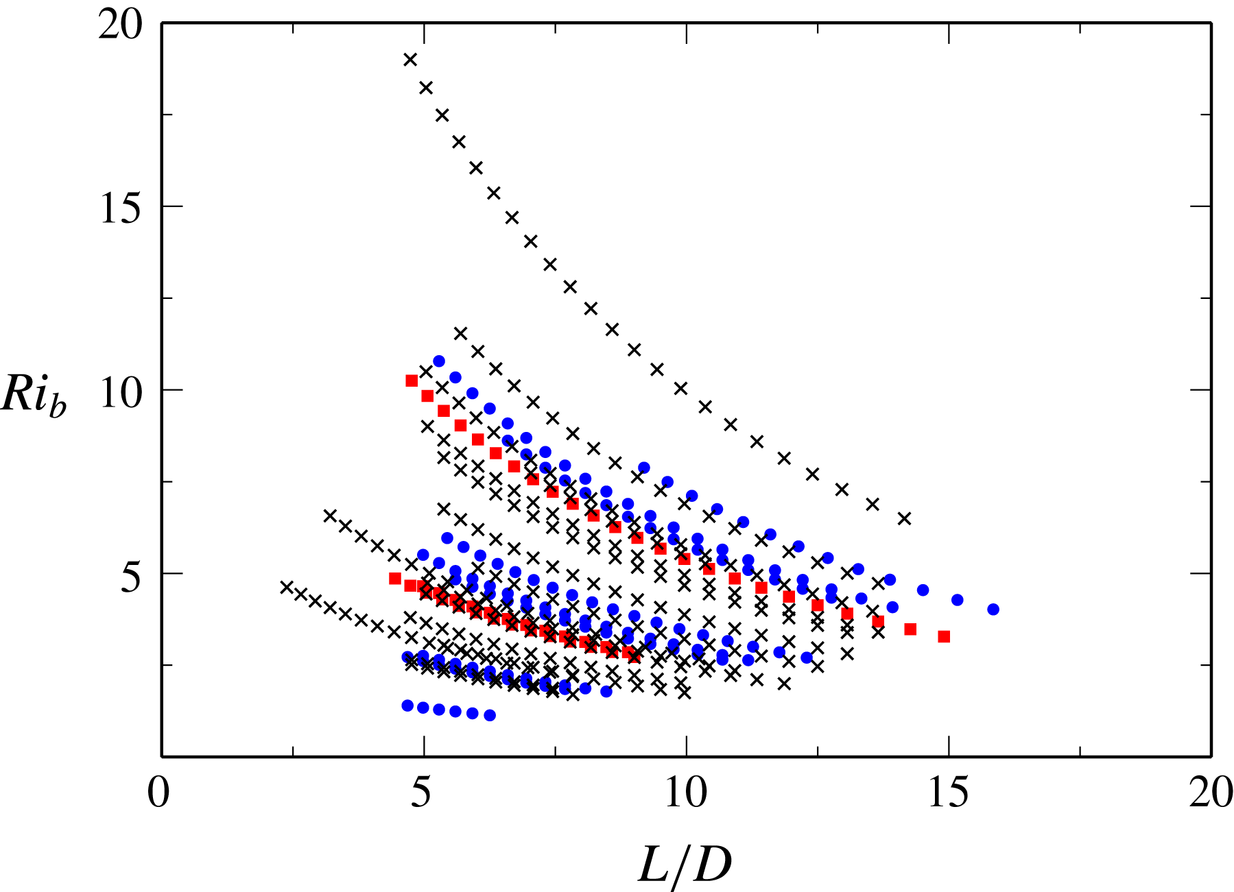
, are time varying, as the interface is eroded during these experiments. The total parametric range covered within the experiments is
 $Ri_{b}=1.1$
to 19 and
 $L/D=2.4$
to 16, as illustrated in figure 2.
Experiments performed with instantaneous realisations of time-varying
 $Ri_{b}$
and flow aspect ratio
 $L/D$
at Reynolds numbers of
 $Re=7100$
(●) (blue),
 $Re=11\,300$
(
 $\times$
) (black) and
 $Re=15\,100$
(▪) (red).

The interface depth was measured using dye visualisation. The cavity was illuminated by stage lights behind a diffuse screen attached to the back surface of the flume. A weak solution of food dye was used as a passive tracer in the saline cavity fluid. A camera, with a side view of the cavity interface, recorded images of the 200 mm square region at the centre of the cavity at 1 Hz. Each image in the sequence was averaged horizontally to obtain a mean vertical profile of light intensity. The peak gradient in image intensity was used to locate the density interface and measure the interface depth
 $D$
. The interface length
 $L$
, interface area
 $LB$
and the mixed layer velocity
 $U_{b}=U_{0}H/D$
can then be obtained directly. In the re-circulating channel flow, the mixed layer salinity increases as a result of entrainment from the cavity, so the density difference
 $\unicode[STIX]{x0394}\unicode[STIX]{x1D70C}/\unicode[STIX]{x1D70C}_{0}$
decreases slightly with time.
The rig was instrumented with three temperature/conductivity probes at the upstream
 $TC_{1}$
location and downstream
 $TC_{2,3}$
location, as noted in figure 1. The flow in the downstream straight section was homogenised by small turbulence promoters in the exit section before the
 $TC_{2,3}$
probes. The two downstream probes are fast-response temperature conductivity probes (model 125 MicroScale (MSCTI) made by Precision Measurement Engineering) which record the flow conductivity and temperature. The upstream probe is a Kenek MK-103 (Keisoku Giken Co. Ltd). All probes were logged at 100 Hz through a NI cDAQ board to a PC. All probes were calibrated with known saline solutions before and after each experiment, with a third-order regression fit used to obtain the solution salinity,
 $\unicode[STIX]{x1D70E}$
. The correction for temperature effects of conductivity were made using the linear temperature conductivity relations from Hewitt (Reference Hewitt1960). The MSCTII probes have a linear voltage response to conductivity from 0.5 to
 $800~\text{mS}~\text{cm}^{-1}$
, which leads to a lower measurement limit at
 $18~^{\circ }\text{C}$
of approximately
 $0.3~\text{g}~\text{NaCl}~\text{L}^{-1}$
. Salinity and
 $D(t)$
measurements were averaged over a period of 20 s to obtain smooth time series. The
 $TC_{1}$
probe is used to measure the time-varying
 $\unicode[STIX]{x0394}\unicode[STIX]{x1D70C}/\unicode[STIX]{x1D70C}_{0}$
and
 $Ri_{b}$
.
The entrainment velocity
 $u_{e}$
was obtained using three approaches. The first measure was obtained using the change in interface depth as
 $$\begin{eqnarray}u_{e,\unicode[STIX]{x1D6FF}h}=\text{d}V/\text{d}t(1/LB),\end{eqnarray}$$
where
 $V$
is the remaining volume of saline solution in the cavity. This method has been used successfully in previous studies (Debler & Armfield Reference Debler and Armfield1997; Kirkpatrick & Armfield Reference Kirkpatrick and Armfield2005). A second measurement approach takes the difference in salinity recorded across the cavity
 $\unicode[STIX]{x1D70E}_{1}$
and
 $\unicode[STIX]{x1D70E}_{2,3}$
at probes
 $TC_{1}$
and
 $TC_{2,3}$
. Taking a balance of salt content within a control volume in the overflow extending from the cavity interface up to the free surface and integrating over the time it takes for fluid to pass through the volume,
 $\unicode[STIX]{x0394}t$
, we obtain the balance to a second-order approximation,
 $$\begin{eqnarray}\frac{\text{d}\unicode[STIX]{x1D70E}LD}{\text{d}t}=\unicode[STIX]{x1D70E}_{c}Lu_{e}+\unicode[STIX]{x1D70E}_{c}\frac{\text{d}u_{e}L}{\text{d}t}\frac{\unicode[STIX]{x0394}t}{2}-\left(U_{b}H\unicode[STIX]{x1D70E}_{e}+\frac{\text{d}U_{b}H\unicode[STIX]{x1D70E}_{e}}{\text{d}t}\frac{\unicode[STIX]{x0394}t}{2}-U_{b}H\unicode[STIX]{x1D70E}_{i}-\frac{\text{d}U_{b}H\unicode[STIX]{x1D70E}_{i}}{\text{d}t}\frac{\unicode[STIX]{x0394}t}{2}\right),\end{eqnarray}$$
where
 $\unicode[STIX]{x1D70E}$
is the salinity within the control volume,
 $\unicode[STIX]{x1D70E}_{i}$
and
 $\unicode[STIX]{x1D70E}_{e}$
are the salinity of the overflow entering and leaving the control volume respectively, the values of which can be obtained by a temporal shift in the time series
 $\unicode[STIX]{x1D70E}_{1}(t)$
and
 $\unicode[STIX]{x1D70E}_{2,3}(t)$
by the advection time
 $\unicode[STIX]{x1D70F}$
from the measurement locations to the limits of the control volume. This is implemented as a shift in both upstream and downstream signals to the cavity location, consistent with our
 $D(t)$
and
 $L(t)$
measurements at time
 $t$
. The advection time
 $\unicode[STIX]{x0394}t$
is small
 $O(10~\text{s})$
compared with the experiment time
 $O(1000~\text{s})$
over which entrainment is varying so we neglect the
 $\text{d}\unicode[STIX]{x1D70E}LD/\text{d}t$
term and those in
 $\unicode[STIX]{x0394}t$
to obtain a first-order approximation of the entrainment rate,
 $$\begin{eqnarray}u_{e}=U_{b}H[\unicode[STIX]{x1D70E}_{2,3}(t-\unicode[STIX]{x1D70F}_{2,3})-\unicode[STIX]{x1D70E}_{1}(t+\unicode[STIX]{x1D70F}_{1})]/(L(t)\unicode[STIX]{x1D70E}_{c}),\end{eqnarray}$$
where
 $\unicode[STIX]{x1D70F}_{1}$
and
 $\unicode[STIX]{x1D70F}_{2,3}$
are the advection time between the centre of the cavity and the probe locations. A third measure of entrainment was also obtained using the rate of change of salinity in the
 $\unicode[STIX]{x1D70E}_{1}(t)$
series. The re-circulating flow stream increases in salinity with time, which allows the entrainment rate to be obtained from (3.4) using an estimate for the downstream salinity
 $\unicode[STIX]{x1D70E}_{2,3}(t)$
obtained from a salinity mass balance on the reservoir,
 $$\begin{eqnarray}\unicode[STIX]{x1D70E}_{2,3}=\frac{\text{d}\unicode[STIX]{x1D70E}_{r}}{\text{d}t}\frac{V_{r}}{Q}\unicode[STIX]{x1D6FD}+\unicode[STIX]{x1D70E}_{r}.\end{eqnarray}$$
Here
 $V_{r}$
is the reservoir volume and
 $Q$
is the flow rate. The salinity of the reservoir
 $\unicode[STIX]{x1D70E}_{r}$
is obtained by a temporal shift in the
 $\unicode[STIX]{x1D70E}_{1}$
time series,
 $\unicode[STIX]{x1D70E}_{r}=\unicode[STIX]{x1D70E}_{1}(t-\unicode[STIX]{x1D70F}_{r})$
, where
 $\unicode[STIX]{x1D70F}_{r}$
is the time taken for the fluid to be pumped from the reservoir to the probe at location 1. The time derivative of this signal,
 $\text{d}\unicode[STIX]{x1D70E}_{r}/\text{d}t$
, is taken over the measurement averaging period of 20 s. We have introduced a constant
 $\unicode[STIX]{x1D6FD}$
which is
 $\simeq 1.0$
, indicating nearly complete mixing in the reservoir. This fitting constant is obtained directly from the flow for every
 $Q$
and
 $V_{r}$
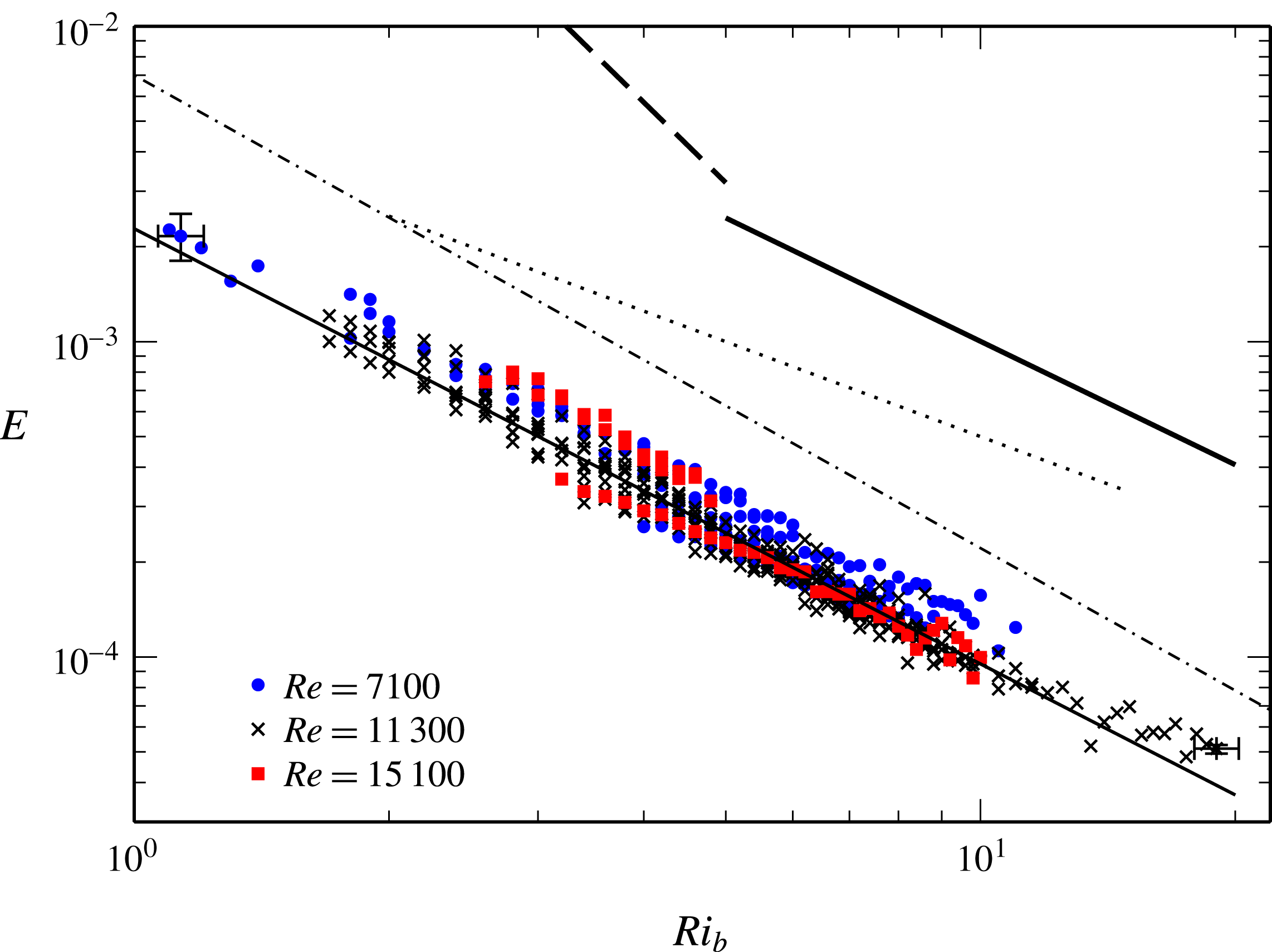
setting used. Both instantaneous and continuous releases of fluid from the cavity and at the entrance to the reservoir were used to determine the accuracy of the method. The method simplifies the rig instrumentation, which is an advantage when performing other types of experiments such as simultaneous PIV/PLIF work. Unless otherwise stated the results presented were obtained with this method. Measurements obtained from method 1, 2 and 3 are consistent with both the direct tests from controlled releases and results obtained during the experiments. We have indicated error bars expected from the accuracy of the instruments in figure 3. These error bars indicate scatter is of the same magnitude as the expected bounds of error.
Entrainment rate
 $E=u_{e}/U$
for all data with
 $Re=7100$
(●) (blue),
 $Re=11\,300$
(
 $\times$
) (black) and
 $Re=15\,100$
(▪) (red). The thin solid black line indicates
 $E=CRi^{n}$
, where
 $C=0.0023$
and
 $n=-1.38$
. Data from Strang & Fernando (Reference Strang and Fernando2001) are given by the thick dashed line (
 $C=0.22$
,
 $n=-2.63$
) and the thick solid line (
 $C=0.02$
,
 $n=-1.3$
). Data of Narimousa & Fernando (Reference Narimousa and Fernando1987) are given by the thin dotted line (
 $C=0.005$
,
 $n=-1$
) and the relationship of Christodoulou (Reference Christodoulou1986) given by the thin dash-dotted line (
 $C=0.007$
,
 $n=-1.5$
).

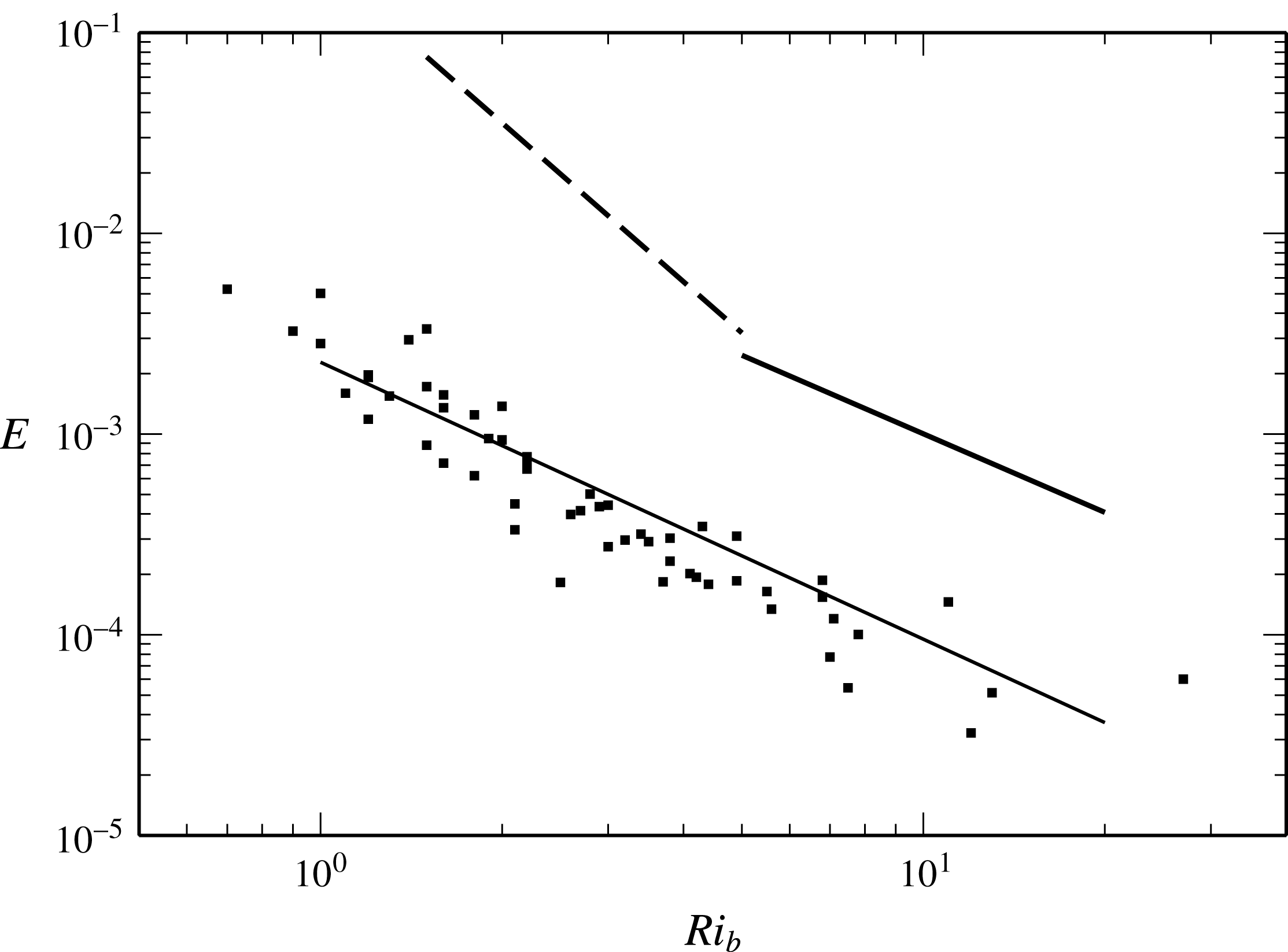
Entrainment rate data of Deardorff & Willis (Reference Deardorff and Willis1982) (▪) for two-layer stratified fresh/saline water flow. Lines are as indicated in figure 3.

3.1 Entrainment rate with
 $Ri_{b}$

The entrainment rate results for all the data collected are presented in figure 3 with the three Reynolds number values indicated. It is immediately clear that within the data presented there is a single entrainment regime across the entire
 $Ri_{b}$
range. Within our Reynolds number range we are unable to discern a significant sensitivity of entrainment to this parameter. We obtain a regression fit of
 $E=CRi_{b}^{n}$
, with
 $n=-1.38$
and
 $C=0.0023\pm 0.0007$
, for the more extensive
 $Re=11\,300$
results. Entrainment measurements obtained using (3.2) for the same experiments give
 $n=-1.35$
and
 $C=0.0022\pm 0.0007$
(data not shown). The estimates of experimental error in the calculation of
 $Ri_{b}$
and
 $E$
are indicated by error bars in the figure. In the same figure we present the entrainment correlations of Strang & Fernando (Reference Strang and Fernando2001) obtained using an Odell–Kovasznay type re-circulating water channel. In their regime 2 over
 $Ri_{b}=1.5$
to 5 they observed
 $E\simeq CRi_{b}^{n}$
, where
 $C_{2}\simeq 0.22\pm 0.11$
and
 $n\simeq -2.63\pm 0.45$
. At higher Richardson number, in their regime 3 over
 $Ri_{b}=5-20$
, they found
 $C_{3}\simeq 0.02\pm 0.01$
and
 $n\simeq -1.3\pm 0.15$
. Our exponent
 $n=-1.38$
lies within the range of values they report for their regime 3, but our constant
 $C$
is approximately an order of magnitude smaller and we observe this scaling holds down to
 $Ri_{b}\simeq 1$
. The consistency among the exponent values between the studies suggests that similar mechanisms may be present, that is in both flows entrainment is a result of shear-driven effects at the interface rather than cavity-related mechanisms, and that the entrainment regime is related to the
 $Ri_{b}>5$
regime reported by Strang & Fernando (Reference Strang and Fernando2001). Also shown is the empirical result (
 $C=0.007$
,
 $n=-1.5$
) obtained by Narimousa & Fernando (Reference Narimousa and Fernando1987) in an Odell–Kovasznay water channel over
 $Ri_{b}=2$
to 15 and the relationship obtained by Christodoulou (Reference Christodoulou1986) (
 $C=0.007$
,
 $n=-1.5$
), who re-interpreted data from a range of earlier studies of two-layer shear flows including the buoyant wall jet data of Lofquist (Reference Lofquist1960) and screen-driven annulus data of Kantha et al. (Reference Kantha, Phillips and Azad1977). The data set included no cavity flow configurations. The exponent obtained by Christodoulou (Reference Christodoulou1986) is consistent with our measurements and those of Strang & Fernando (Reference Strang and Fernando2001), although the coefficient is again larger in this data set.
The entrainment data of Deardorff & Willis (Reference Deardorff and Willis1982) are plotted over our regression fit in figure 4. In the annulus configuration, entrainment has an additional dependency on annulus curvature (Scranton & Lindberg Reference Scranton and Lindberg1983) such that, with increasing curvature, turbulence in the mixed layer is damped, resulting in a reduction in mixing at the interface (Deardorff & Yoon Reference Deardorff and Yoon1984). Interestingly this data set is similar to our result both in terms of the magnitude and in terms of the
 $Ri_{b}$
range for this entrainment regime. We further investigate the origins of the reduced mixing in the present results in § 4.
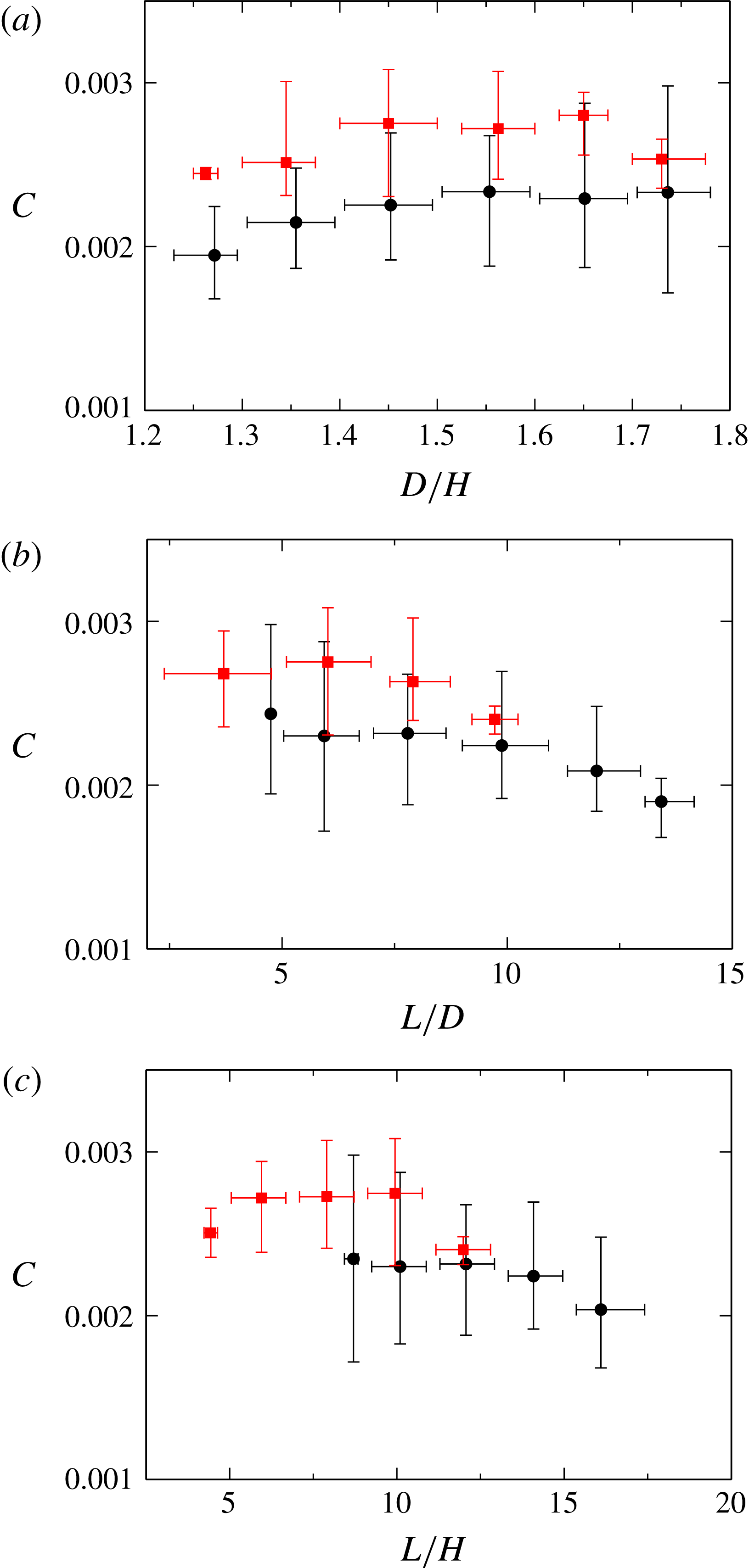
Coefficient
 $C=ERi^{1.38}$
with flow aspect ratio
 $D/H$
(a),
 $L/D$
(b) and
 $L/H$
(c) for
 $l_{c}=2.1$
(●) (black) and
 $l_{c}=1.6$
(▪) (red) for
 $Re=11\,300$
. Mean values plotted, with bars giving the range of data.

Our entrainment measurements are binned into bands of the geometric ratios
 $D/H$
,
 $L/D$
and
 $L/H$
, plotted in figure 5(a–c), respectively. Here the arithmetic mean of the coefficient
 $C$
for the data within each bin and the range of data are indicated by the horizontal bars in the figure. The vertical bars indicate the range of
 $C$
in each bin. The data for the
 $l_{c}=2.1~\text{m}$
and
 $l_{c}=1.6~\text{m}$
experiments are plotted separately in the figure. Initially we note that in figure 5(a) the variation in the coefficient
 $C$
with
 $D/H$
is shown to be small, confirming that entrainment has no significant dependency on the upstream channel depth or the cavity depth
 $K$
, recalling that
 $(K+D)/H$
is a constant. The variation in the mean value of
 $C$
with
 $L/D$
or
 $L/H$
, plotted in figure 5(b) and 5(c), is generally within the scatter of the data at each geometric ratio. The mean value of
 $C$
in the
 $l_{c}=1.6~\text{m}$
data set is somewhat higher than that of the
 $l_{c}=2.1~\text{m}$
data set across all common values of
 $L/D$
or
 $L/H$
, but these differences are less than the ranges within each bin. At large values of
 $L/D$
and
 $L/H$
, the data set is smaller, so the reduction in the mean value of
 $C$
and the scatter should be treated with caution. The figures show that at least until
 $L/D=14$
, a single bulk Richardson number and set of constants
 $C$
and
 $n$
are effective parameters to characterise the flow along the entire length of the interface. This may be interpreted as evidence that the entrainment across the interface varies insignificantly along the length of the interface over this range. We make two inferences from this observation.
Firstly, the insensitivity of bulk entrainment to interface length suggests similar insensitivity of interfacial mixing at the interface over its length. The excitation of the interface by turbulence is expected to enhance or initiate interfacial mixing and entrainment in combination with local shear and wave activity in the cavity. Turbulence in the mixed layer is both transported from the upstream channel flow and generated locally in the cavity section by shear or buoyancy production. We may infer that these mechanisms are insensitive to cavity length or distance from the upstream channel.
Secondly, Strang & Fernando (Reference Strang and Fernando2001) demonstrated a clear relationship between entrainment and interface thickness. Our observations that entrainment is insensitive to length imply that in our experiments the interface properties are varying insignificantly over this length. As interface thickness develops in the streamwise direction, starting at the upstream slope with close to zero thickness, this suggests that the interface is very thin over the entire length of the cavity.
This observation is qualitatively confirmed by dye visualisation at the interface and by LIF measurements in § 4. Both the sharp nature of the interface and the
 $n=-1.38$
exponent on the entrainment rate suggest that the flow is behaving similarly to the
 $Ri_{b}>5$
regime of Strang & Fernando (Reference Strang and Fernando2001), where their interface is characterised by Holmboe waves. In our setting, however, this regime appears to extend over our entire experimental range, from
 $Ri_{b}=1$
to 19.
Finally we also note that while the density of the mixed layer increases slightly in the direction of flow, as it receives entrained fluid from the cavity, this variation is negligible, as the low entrainment rate results in a very small dilution of the mixed layer over
 $L/D=14$
.
4 Interface characterisation
Further identification of the entrainment regime and characterisation of the interface properties necessitated local measurements of the interface thickness. We conducted additional experiments at
 $Re=7100$
with the laboratory rig instrumented with a two-dimensional particle image velocimetry (PIV) and laser induced fluorescence (LIF) system to obtain simultaneous time series of the velocity and density fields in vertical planes aligned with the direction of the mean flow.
The simultaneous PIV/LIF system is comprised of a dual-cavity 15 Hz 532 nm Nd:YAG pulsed laser (Quantel Evergreen Big Sky) capable of pulse energies up to 145 mJ. The laser beam passes through lenses to create a collimated light sheet 58 mm wide and
 $\simeq 1~\text{mm}$
thick. The beam is then reflected vertically down into the flume using a plane mirror. A ‘periscope’ with a Perspex base that sits just below the top surface of the water allows the beam to pass through the free surface. The periscope is designed to minimise interference with the flow. It penetrates less than 10 mm below the surface and is located 1300 mm from the upstream end of the cavity. Ethanol is added to the fresh water tank to match the refractive indices between the fresh and salt water. Fluorescence for the LIF imaging was achieved using Rhodamine 6G dye added to the fresh water with a concentration of 20 ppb. The saline water stream has no Rhodamine dye added. For the PIV imaging, natural particles present in the water supply were used as tracer particles. Initial attempts to add additional tracer particles resulted in a significant reduction in LIF image quality as a result of increased scatter of 532 nm light, and hence excitation of the Rhodamine dye, throughout the channel.
Images were recorded using two
 $2048\times 2048$
pixel CCD cameras (PCO.2000, monochrome, double shutter, CCD sensor size
 $15.2\times 15.2~\text{mm}$
) mounted on one side of the cavity section and fitted with AF Micro-NIKKOR 60 mm f/2.8D lenses. The PIV camera is fitted with a 532 nm bandpass interference filter while the LIF camera is fitted with a Kodak Wratten 22 filter with a cutoff wavelength of 550 nm to remove the 532 nm light scattered by the PIV particles. The cameras were positioned to image the density interface layer with a region of interest (ROI) of
 $56\times 100~\text{mm}$
. With this arrangement the camera utilised
 $1400\times 2048~\text{pixels}$
, giving a maximum resolution of
 $0.04~\text{mm}\times 0.04~\text{mm}$
for LIF, adequate to resolve the interface thickness of
 $\unicode[STIX]{x1D6FF}_{b}\simeq 1~\text{mm}$
. The laser sheet has a thickness of
 ${\sim}1~\text{mm}$
so all results are in effect filtered in the spanwise plane. The LIF intensity images
 $I_{r}(x,z,t)$
at time
 $t$
are normalised using the reference concentration image
 $I_{c}(x,z,t)$
and the black level image
 $I_{b}(x,z)$
:
 $$\begin{eqnarray}I(x,z,t)=(I_{r}(x,z,t)-I_{b})/(I_{c}(x,z,t)-I_{b}(x,z)).\end{eqnarray}$$
Variation in laser power is corrected for by using the reference region in the LIF images, extending from
 $y=115$
to
 $y=120~\text{mm}$
, which lies in the mixed layer. An additional calibration is made using the
 $TC_{1}$
upstream conductivity probe which measures the time-varying density in the overflow.
The double-frame PIV images are passed through a fast Fourier transform (FFT) cross-correlation algorithm based on the open-source PIVsuite package, using an interrogation window of
 $32\times 16~\text{pixels}$
, giving a resolution of
 $1.28~\text{mm}\times 0.64~\text{mm}$
. A 50 % overlap in the interrogation windows gives a PIV field of
 $84\times 272$
vectors over a streamwise/vertical plane. The velocity field was interpolated onto the LIF data using a third-order-accurate polynomial. This resolution is adequate to resolve the shear layer, which is shown to be
 $\unicode[STIX]{x1D6FF}_{s}\simeq 9~\text{mm}$
across all the experiments. The image pairs were captured at a frequency of 2 Hz for a total of 449 realisations of the flow per image sequence. A total of 14 image sequences were obtained covering
 $Ri_{b}=2$
to 10.
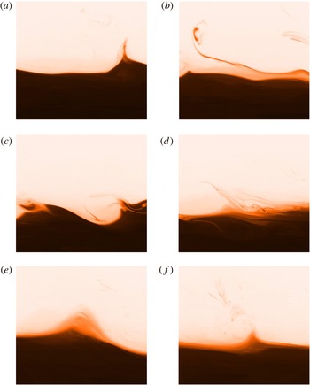
Instantaneous realisations of the density at
 $Ri_{b}=4.1$
,
 $Ri_{g}=27$
and
 $Re=7100$
. The images illustrate streamer formation (a), streamer stretching (b), intermittent engulfment (c), diffuse intermediate region (d), and apparent sharpening of the interface by streamer formation (e) and (f).

Instantaneous realisations of the density field are depicted in figure 6 at
 $Ri_{b}=4.1$
. The two layers are separated by a sharp density interface which is perturbed by waves at a range of wavelengths and amplitudes. Figures 6(a,b,e,f) are classic Holmboe waves. Non-breaking waves are observed to form cusps or peaks which eject thin ‘streamers’ (Kirkpatrick et al.
Reference Kirkpatrick, Armfield and Williamson2012) or ‘wisps’ (Narimousa & Fernando Reference Narimousa and Fernando1987; Carpenter et al.
Reference Carpenter, Tedford, Rahmani and Lawrence2010) of fluid into the mixed layer (figure 6
a,b). Similar ejections of fluid are seen in the experimental and numerical studies of Holmboe waves (e.g. Browand & Winant Reference Browand and Winant1973; Carpenter, Lawrence & Smyth Reference Carpenter, Lawrence and Smyth2007; Tedford, Pieters & Lawrence Reference Tedford, Pieters and Lawrence2009; Carpenter et al.
Reference Carpenter, Tedford, Rahmani and Lawrence2010). Our images show streamers rapidly advected vertically upwards into the mixed layer or along the interface and stretched and occasionally folded back into the lower layer with engulfment of ambient fluid in intermittently occurring overturns, as shown in figure 6(c).
We note that the interface thickness varies only slightly through the image sequence, as seen in the contrasting thickness in figures 6(a) and 6(d). We do not observe a significant intermittent partially mixed interfacial region as was seen by Strang & Fernando (Reference Strang and Fernando2001) for
 $Ri<5$
, where the interface dynamics were characterised by K–H instabilities. In the present study the entrainment of the ejected fluid into the upper layer is rapid while the interface itself remains sharp. The lack of an intermediate layer above the interface suggests that entrainment is limited by mixing at the interface rather than transport from the interface to the overflow as was observed by Strang & Fernando (Reference Strang and Fernando2001). In figures 6(e) and 6(f) we see apparent sharpening of the interfacial region where diffuse interface fluid appears drawn to a peak of a wave crest and entrained into the upper layer, as proposed by Kirkpatrick et al. (Reference Kirkpatrick, Armfield and Williamson2012). The full image sequence is presented as a movie in the supplementary online material available at https://doi.org/10.1017/jfm.2017.796. These qualitative observations appear similar to the wave-breaking-dominated regime reported in the experimental results of Narimousa & Fernando (Reference Narimousa and Fernando1987) for flow at
 $Ri_{b}>5$
, the descriptions of Sullivan & List (Reference Sullivan and List1994) and the images provided by Strang & Fernando (Reference Strang and Fernando2001) for
 $Ri_{b}>5$
flow. As the Richardson number is increased beyond
 $Ri_{b}\simeq 6$
the overturns in the flow were not observed; however, the ejection from non-breaking wave crests in ‘streamers’ continues over the entire experimental range.
It is clear that the amplitude and wavelength of the interfacial waves and overturns exist at scales much larger than the interface thickness, even at relatively low
 $Ri_{b}$
.
4.1 Characterisation of interface
$\unicode[STIX]{x0394}U$
,
$\unicode[STIX]{x0394}\unicode[STIX]{x1D70C}$
and
$L_{21}$


Initially we use the local PIV/LIF measurements to determine how the bulk parameters characterise the flow near the interface. This is in part motivated by the different
 $Ri_{b}$
ranges reported in Strang & Fernando (Reference Strang and Fernando2001) for the Holmboe wave regime and also their higher constant
 $C\simeq 0.02$
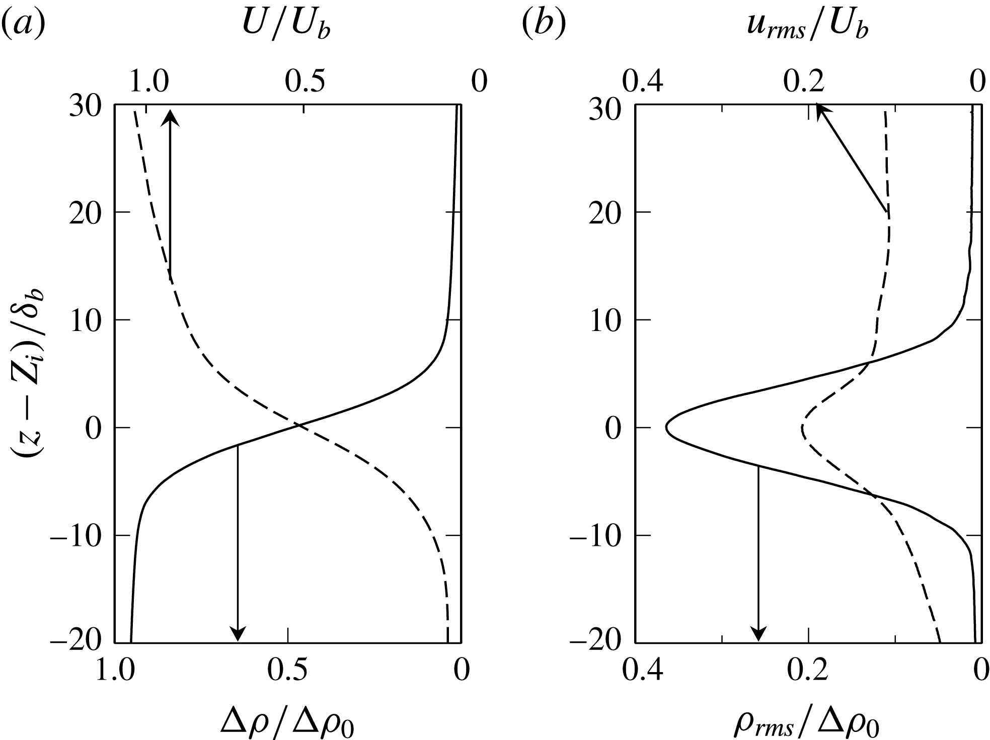
shown in figure 3. The time-averaged density and velocity profiles are shown in figure 7(a) at
 $Ri_{B}=3.3$
, with the vertical location plotted relative to the mean interface depth
 $Z_{i}$
and normalised by the interface thickness
 $\unicode[STIX]{x1D6FF}_{b}$
, defined in (4.4). In § 4.2 we later show conditionally averaged statistics of the same quantities.
The mean density profile clearly illustrates the two-layer structure, defined by the upper turbulent ‘mixed layer’, a thin interface region and a lower dense layer. Density stratification within the mixed layer and lower layer is very low, so normalisation of the density field by
 $\unicode[STIX]{x0394}\unicode[STIX]{x1D70C}_{0}$
is reasonable. The density fluctuations in the mixed and lower layers are very low outside the narrow interface region, as shown in figure 7(b). The mean velocity decreases rapidly below the density interface, and within the lower layer is close to zero. This structure persisted at all the interface depths examined. The normalisation of the velocity field by the bulk velocity
 $U_{b}$
, as shown in figure 7(a), gives a velocity rise of
 $\unicode[STIX]{x0394}U/U_{b}\sim 1$
across the shear layer. Both the bulk scales
 $U_{b}$
and
 $\unicode[STIX]{x0394}\unicode[STIX]{x1D70C}_{0}$
used in the bulk Richardson number are well defined to characterise the flow, so the differences between our results and those of Strang & Fernando (Reference Strang and Fernando2001) for the mapping of the entrainment regime with
 $Ri_{b}$
are not the result of a poor choice in outer scales. At this point we also note that the streamwise turbulence intensity (given in figure 7
b) in the upper layer
 $u_{rms}/U_{b}\simeq 0.14$
is similar to the values present in Strang & Fernando (Reference Strang and Fernando2001). We also estimated the integral length scale of turbulence in the mixed layer using
 $$\begin{eqnarray}L_{21}(z)=\frac{1}{R_{21}(0,z,0)}\int _{0}^{X}R_{21}(x,z,r)\,\text{d}r.\end{eqnarray}$$
Here the cross-correlation coefficient
 $R_{21}(x,z,r)=\overline{w^{\prime }(x,z)w^{\prime }(x+r,z)}$
, where
 $w^{\prime }$
is the fluctuation in the vertical velocity component,
 $x$
is the distance in the streamwise direction,
 $X$
is the width of the PIV velocity field data, and the overline denotes an average over the image sequence. In this range the integral length scale as defined, normalised by mixed layer depth
 $L_{21}/D\simeq 0.2$
, is also similar to the value of
 $L_{11}/D\simeq 0.18$
obtained by Strang & Fernando (Reference Strang and Fernando2001). The Reynolds number ranges of the two studies are also of the same order
 $Re\sim O(10^{4})$
.
Mean streamwise velocity profile, density (a) and r.m.s. density fluctuation
 $(\unicode[STIX]{x1D719}^{\prime }\unicode[STIX]{x1D719}^{\prime })^{1/2}/(\unicode[STIX]{x1D719}-\unicode[STIX]{x1D719}_{0})$
and turbulence intensity (b) at
 $Ri_{b}=3.3$
,
 $Ri_{g}=19$
, averaged over
 $\unicode[STIX]{x1D70F}=224~\text{s}$
.

4.2 Characterisation of interface
$\unicode[STIX]{x1D6FF}_{b}$
and
$\unicode[STIX]{x1D6FF}_{s}$


The instantaneous interface thickness properties were interrogated using a conditional average of the flow field which has been shifted relative to the local interface height. The instantaneous interface location vector
 $[x_{i},z_{i}]$
was obtained using an interface tracking tool that traces the contour of
 $0.5(\unicode[STIX]{x1D719}_{1}-\unicode[STIX]{x1D719}_{0})$
across the image, where
 $\unicode[STIX]{x1D719}_{1}$
is the scalar concentration of the mixed layer and
 $\unicode[STIX]{x1D719}_{0}$
that in the lower layer. The interface is tracked such that there is one contiguous interface between the two layers. This interface does not include secondary interfaces formed where wholly detached regions of dense flow are entrained into the overflow or light fluid is engulfed into the lower dense layer by overturns. In the automated procedure the interface is located on one side of the image and tracked across the image until the opposing edge is reached. The interface coordinates are stored as a vector
 $\boldsymbol{C}_{i}=[x_{i},z_{i}]$
. Where there is an overturn in the interface, multiple values of
 $x_{i}$
will exist in the
 $\boldsymbol{C}_{i}$
for that image.
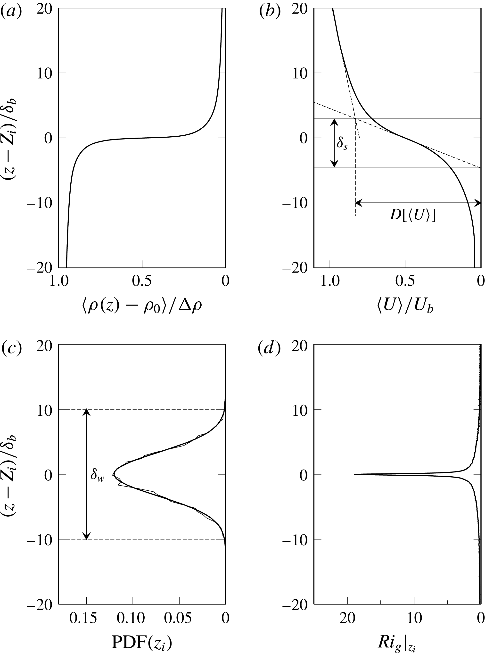
Conditionally averaged density (a) and velocity (b), PDF of the interface location
 $z_{i}$
(thin solid line) with a Gaussian fit (thick solid line) (c), and the
 $Ri_{g}$
profile (d). Data are presented for a single image sequence with
 $Ri_{b}=3.3$
,
 $Ri_{g}=19$
and
 $\unicode[STIX]{x1D6FF}_{s}/\unicode[STIX]{x1D6FF}_{b}=10.7$
.

We obtained
 $\unicode[STIX]{x1D6FF}_{s}$
and
 $\unicode[STIX]{x1D6FF}_{b}$
by conditionally averaging the velocity and density fields across all images within an image sequence. This was achieved by taking each interface coordinate in the vector
 $\boldsymbol{C}_{i}$
and shifting the flow field at that
 $x_{i}$
location vertically so that
 $z$
is centred on
 $Z_{i}$
. The profiles are then averaged and plotted against displacement from the interface
 $z-Z_{i}$
. Conditional averaging across all images within an image sequence is indicated by
 $\langle \cdot \rangle$
. In this way velocity and density profiles were obtained relative to the local interface height at each location along the interface. These profiles are given in figures 8(a) and 8(b). We define the shear layer thickness as
 $$\begin{eqnarray}\unicode[STIX]{x1D6FF}_{s}=\frac{\mathscr{D}[\langle U\rangle ]}{\displaystyle \left.\frac{\text{d}\langle U\rangle }{\text{d}z}\right|_{MAX}},\end{eqnarray}$$
where
 $\text{d}\langle U\rangle /\text{d}z|_{MAX}$
is the peak velocity gradient in the interface region. The velocity jump across the interface
 $\mathscr{D}[\langle U\rangle ]$
is the velocity difference between the upper and lower extents of the shear layer. These are obtained from the intersection of three linear fits to the velocity profile, as indicated in figure 8(b). The upper limit of the shear layer is located from the intersection of a linear fit to the velocity profile at the centre of the shear layer
 $z_{s}$
, where
 $z_{s}$
is the location of
 $\text{d}\langle U\rangle /\text{d}z|_{MAX}$
, with a linear fit to the velocity profile in the upper layer. The lower limit of the shear layer is obtained from the intersection of the linear fit through the centre of the interface and
 $\langle U\rangle =0$
. The mixing layer thickness is similarly obtained by
 $$\begin{eqnarray}\unicode[STIX]{x1D6FF}_{b}=\frac{\mathscr{D}[\langle B\rangle ]}{\displaystyle \left.\frac{\text{d}\langle B\rangle }{\text{d}z}\right|_{MAX}},\end{eqnarray}$$
where
 $\mathscr{D}[\langle B\rangle ]$
is the difference in buoyancy in the upper and lower layers measured at the upper and lower extents of the flow field. With these definitions we obtain
 $\unicode[STIX]{x1D6FF}_{s}=8.4~\text{mm}$
and
 $\unicode[STIX]{x1D6FF}_{b}=0.78~\text{mm}$
for the data sequence given in figures 8(a) and 8(b). Across this experimental range from
 $Ri_{b}=2$
to 10 we find relatively small variation in interface thickness with ranges of
 $\unicode[STIX]{x1D6FF}_{b}=0.76~\text{mm}$
to
 $\unicode[STIX]{x1D6FF}_{b}=1.5~\text{mm}$
and with
 $\unicode[STIX]{x1D6FF}_{s}=8.2~\text{mm}$
to
 $\unicode[STIX]{x1D6FF}_{s}=12.8~\text{mm}$
. The centre of the shear layer and density interface are nearly coincident, with the offset distance being
 $z_{s}-Z_{i}=\unicode[STIX]{x1D6FF}_{d}=0.04~\text{mm}$
for this data set, which is within the resolution of our PIV measurements. Across all results we find the offset varies between
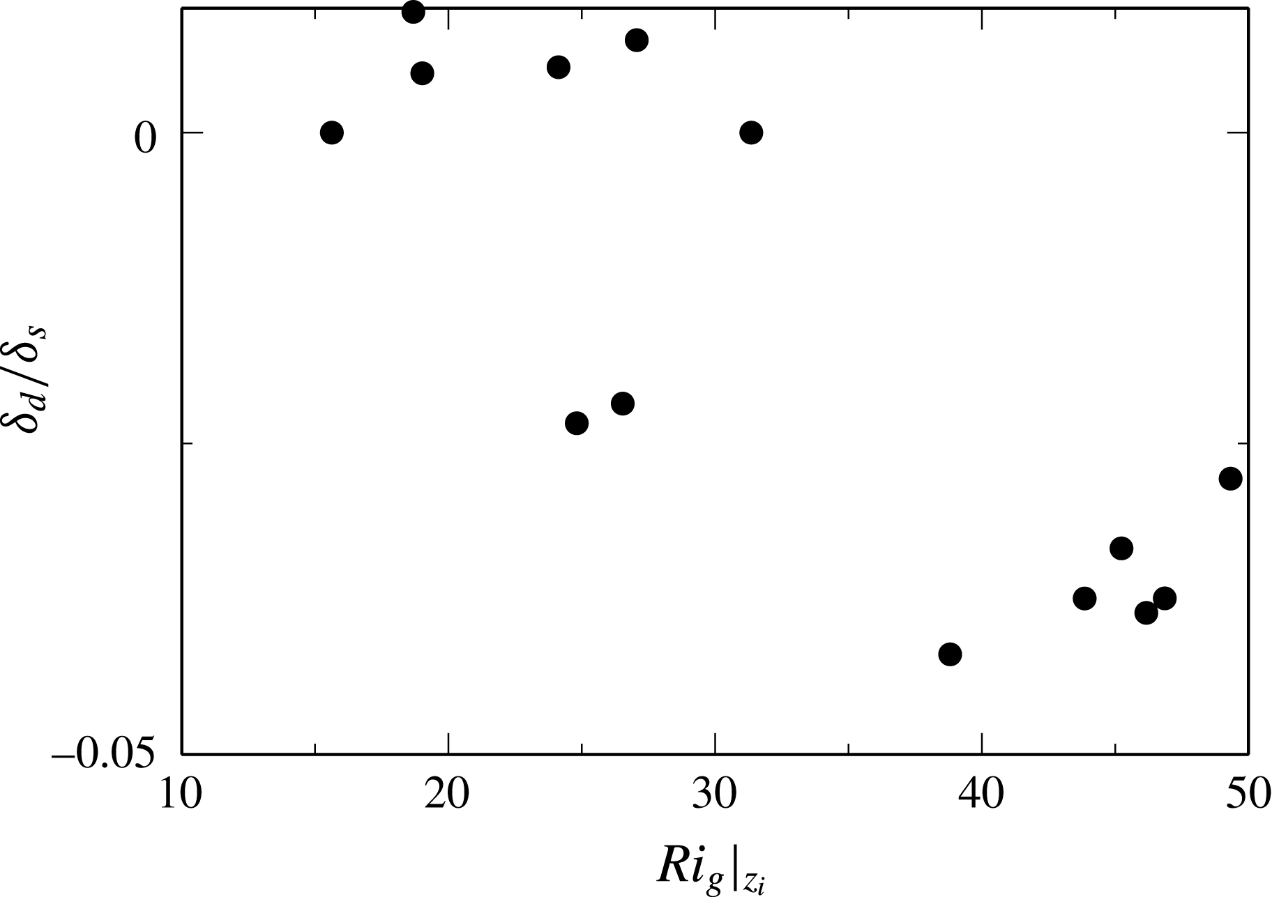
 $\unicode[STIX]{x1D6FF}_{d}/\unicode[STIX]{x1D6FF}_{s}\simeq 0.01$
and
 $-0.05$
. The data shown in figure 9 indicate a similar trend to those shown in Strang & Fernando (Reference Strang and Fernando2001), although extended to higher
 $Ri_{g}$
values in our study.
Ratio of
 $\unicode[STIX]{x1D6FF}_{d}/\unicode[STIX]{x1D6FF}_{s}$
versus the gradient Richardson number at the centre of the interface
 $Ri_{g}|_{z_{i}}$
.

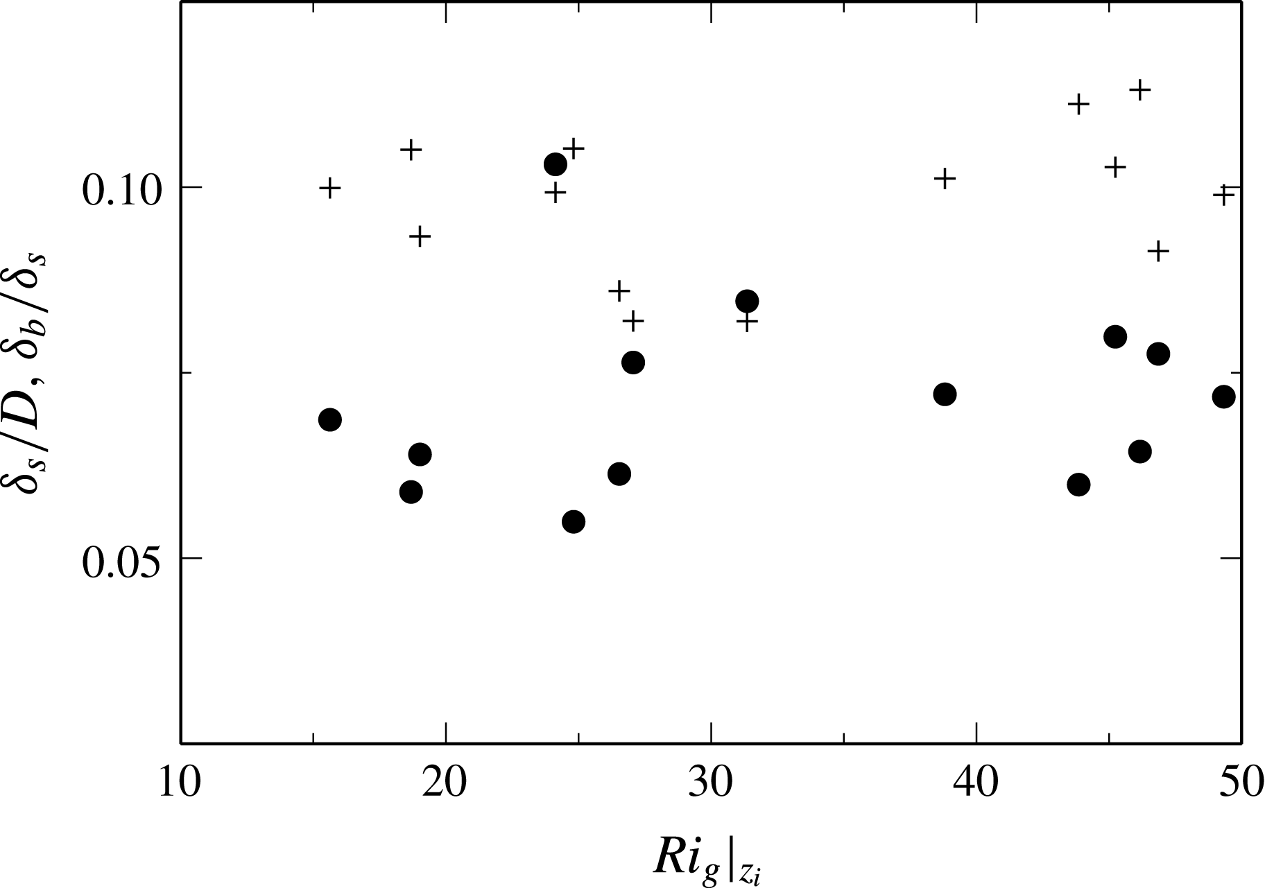
Ratio of length scales
 $\unicode[STIX]{x1D6FF}_{s}/D$
(●) and
 $\unicode[STIX]{x1D6FF}_{b}/\unicode[STIX]{x1D6FF}_{s}$
(
 $+$
) with
 $Ri_{g}|_{z_{i}}$
.

The PDF (probability density function) has been obtained from the concatenated
 $z_{i}$
location data, obtained from each image within an image sequence. The PDF given in figure 8(c) for
 $Ri_{b}=3.3$
shows the function is well approximated by a Gaussian profile,
 $p(z)=ae^{(z-Z_{i})/2c^{2}}$
, where
 $Z_{i}$
is the mean interface height and
 $c$
the standard deviation of
 $z_{i}$
. Using this result we can form a length scale
 $\unicode[STIX]{x1D6FF}_{w}=6c$
, which is an indicator of maximum interface oscillation amplitude. For the
 $Ri_{b}=3.3$
result, shown in figure 8(d),
 $\unicode[STIX]{x1D6FF}_{w}\simeq 20~\text{mm}$
, which is much larger than either the shear layer thickness
 $\unicode[STIX]{x1D6FF}_{s}$
or interface thickness
 $\unicode[STIX]{x1D6FF}_{b}$
. The interface oscillation amplitude
 $\unicode[STIX]{x1D6FF}_{w}$
decreases with increasing
 $Ri_{b}$
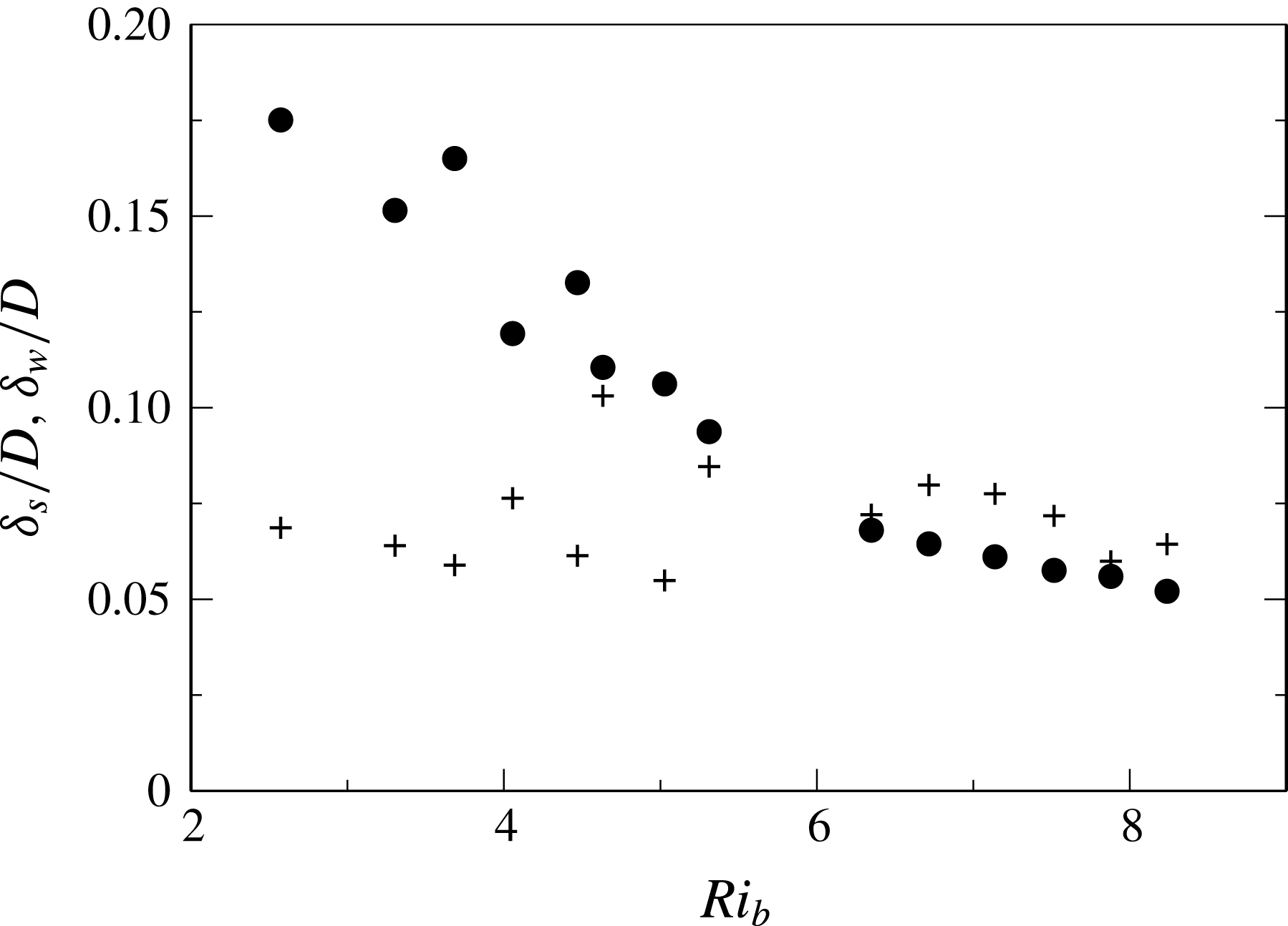
, as shown in figure 11. In the same figure
 $\unicode[STIX]{x1D6FF}_{s}$
is shown to be relatively constant and at
 $Ri_{b}\simeq 6$
the shear layer thickness and the wave amplitude are of similar magnitude,
 $\unicode[STIX]{x1D6FF}_{s}\simeq \unicode[STIX]{x1D6FF}_{w}$
. In turbulent shear free entrainment flows, the interface wave peak height has been shown to be related to the kinetic energy of the impinging eddies (Xuequan & Hopfinger Reference Xuequan and Hopfinger1986). In the present context, however, we are unable to see any consistent relationship between
 $\unicode[STIX]{x1D6FF}_{w}$
and
 $u_{rms}^{2}/\unicode[STIX]{x0394}b$
. Furthermore we do not see any correlation between
 $Ri_{b}$
and a Richardson number based on mixed layer turbulence scales
 $Ri_{L}=\unicode[STIX]{x0394}bL_{12}/u_{rms}^{2}$
in these results.
Length scales
 $\unicode[STIX]{x1D6FF}_{w}/D$
(●) and
 $\unicode[STIX]{x1D6FF}_{s}/D$
(
 $+$
) with
 $Ri_{b}$
.

4.3 Entrainment with
$Ri_{g}$

The average gradient Richardson number is obtained as
 $$\begin{eqnarray}Ri_{g}=\frac{\displaystyle \frac{g}{\unicode[STIX]{x1D70C}_{0}}\left\langle \frac{\unicode[STIX]{x2202}\unicode[STIX]{x1D70C}}{\unicode[STIX]{x2202}z}\right\rangle }{\displaystyle \left\langle \left(\frac{\unicode[STIX]{x2202}U}{\unicode[STIX]{x2202}z}\right)^{2}\right\rangle }.\end{eqnarray}$$
The vertical profile of
 $Ri_{g}$
given in figure 8(d) indicates the maximum value of
 $Ri_{g}$
is located on the interface at height
 $z_{i}$
, with rapid reduction over
 ${\sim}10\unicode[STIX]{x1D6FF}_{b}$
. This profile is characteristic of the Holmboe mode (e.g. Smyth & Winters Reference Smyth and Winters2003). We denote the gradient Richardson number at the centre of the interface
 $Ri_{g}|_{z_{i}}$
. An interesting dynamic in the present results is that the ratio of the shear layer thickness and the mixing layer thickness is nearly constant, with
 $\unicode[STIX]{x1D6FF}_{s}/\unicode[STIX]{x1D6FF}_{b}\simeq 10$
, as shown in figure 10 over
 $Ri_{b}=2$
to 10. Hogg & Ivey (Reference Hogg and Ivey2003) obtained the scaling
 $\unicode[STIX]{x1D6FF}_{s}/\unicode[STIX]{x1D6FF}_{b}\sim Sc^{1/3}$
by considering the contribution of molecular diffusion to the growth of the interface thickness and shear layer thickness over a fixed development length. The authors found good agreement with this scaling using laboratory measurements of a stratified exchange flow. The comparison is also close for our flow, where this scaling predicts a ratio of
 $\unicode[STIX]{x1D6FF}_{s}/\unicode[STIX]{x1D6FF}_{b}\simeq 9$
.
Figure 10 also suggests that
 $\unicode[STIX]{x1D6FF}_{s}/D$
is constant for the present results, as seen in other studies (Narimousa & Fernando Reference Narimousa and Fernando1987; Strang & Fernando Reference Strang and Fernando2001). These quantities are related to
 $Ri_{g}|_{z_{i}}$
as
 $$\begin{eqnarray}Ri_{g}|_{z_{i}}\sim \frac{\unicode[STIX]{x0394}b/\unicode[STIX]{x1D6FF}_{b}}{(U_{b}/\unicode[STIX]{x1D6FF}_{s})^{2}},\end{eqnarray}$$
which implies
 $Ri_{g}|_{z_{i}}\sim Ri_{b}$
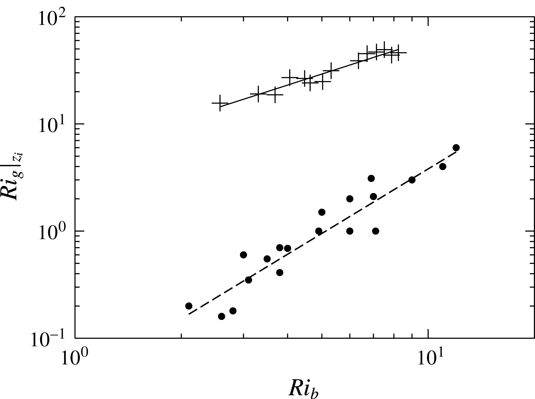
. This relationship is observed in figure 12 with a regression fit of
 $Ri_{g}|_{z_{i}}=5.3Ri_{b}^{1.06}$
. In the same figure the results from Strang & Fernando (Reference Strang and Fernando2001) are presented together with a regression line of
 $Ri_{g}=0.038Ri_{b}^{2}$
. Across the entire experimental range our interface remains sharper with a high gradient Richardson number. The significant variation between the studies is notable; however, exact comparison is difficult, as our results are conditionally averaged about the interface to remove effects of large-scale interfacial waves.
Gradient Richardson number at the centre of the interface
 $Ri_{g}|_{z_{i}}$
versus
 $Ri_{b}$
(
 $+$
) presented with the measurements of Strang & Fernando (Reference Strang and Fernando2001) (●) (taken from their figure 5). Regression lines of
 $Ri_{g}|_{z_{i}}=mRi_{b}^{n}$
are given with
 $m=5.3$
and
 $n=1.06$
for our data (solid line) and
 $m=0.038$
,
 $n=2.0$
for the data of Strang & Fernando (Reference Strang and Fernando2001) (dashed line).

With a shear Richardson number
 $Ri_{s}=\unicode[STIX]{x0394}b\unicode[STIX]{x1D6FF}_{s}/\unicode[STIX]{x0394}U^{2}>0.071$
,
 $\unicode[STIX]{x1D6FF}_{d}/d=0$
and
 $\unicode[STIX]{x1D6FF}_{b}/\unicode[STIX]{x1D6FF}_{s}\rightarrow \infty$
, Holmboe (Reference Holmboe1962) showed using inviscid linear stability analysis that the flow was not unstable to K–H waves but that another mode of instability, the Holmboe wave, was amplified. This mode has since been seen experimentally and numerically (Smyth, Klaassen & Peltier Reference Smyth, Klaassen and Peltier1988; Carpenter et al.
Reference Carpenter, Lawrence and Smyth2007; Tedford et al.
Reference Tedford, Pieters and Lawrence2009; Carpenter et al.
Reference Carpenter, Tedford, Rahmani and Lawrence2010; Salehipour et al.
Reference Salehipour, Caulfield and Peltier2016). In the present study,
 $\unicode[STIX]{x0394}U\simeq U_{b}$
and
 $\unicode[STIX]{x1D6FF}_{s}\simeq 0.07D$
, so we obtain
 $Ri_{s}\simeq 0.07Ri_{b}$
. Over our experimental range of
 $1<Ri_{b}<19$
the flow is above the
 $Ri_{s}=0.07$
limit for K–H waves. The infrequent overturns and lack of clear K–H billows in our flow visualisation is then consistent with stability analysis, not withstanding the highly perturbed and turbulent nature of the cavity flow and variation in velocity and density profiles. The extent of this regime for
 $Ri_{b}<5$
is in contrast to the studies of Narimousa & Fernando (Reference Narimousa and Fernando1987) and Strang & Fernando (Reference Strang and Fernando2001). We have shown that the bulk parameters
 $U_{b}$
and
 $\unicode[STIX]{x0394}\unicode[STIX]{x1D70C}_{0}$
correctly characterise the problem and that turbulence in the mixed layer is similar, i.e. the magnitude of the turbulence intensity and the integral length scale are comparable.
One difference is the configuration, with the cavity setting being a spatially developing flow where the mixing layer has a finite growth time, leading to a flow where
 $\unicode[STIX]{x1D6FF}_{b}$
remains thin and is not correlated with the bulk parameters
 $D$
in the same way as a more developed flow such as is achieved in the re-circulating water channel results obtained by Kantha et al. (Reference Kantha, Phillips and Azad1977), Narimousa & Fernando (Reference Narimousa and Fernando1987) and Strang & Fernando (Reference Strang and Fernando2001). The same behaviour was shown by Salehipour et al. (Reference Salehipour, Caulfield and Peltier2016) using direct numerical simulations. The authors simulated two flows with an initial
 $Ri_{b}=0.16$
but with differing
 $\unicode[STIX]{x1D6FF}_{s}/\unicode[STIX]{x1D6FF}_{s}$
. The flow with
 $Ri_{g}=0.16$
developed into K–H waves while the
 $Ri_{g}=0.16\sqrt{8}$
simulation developed into Holmboe waves.
Both our measurements and those of Strang & Fernando (Reference Strang and Fernando2001) (at
 $Ri_{b}>5$
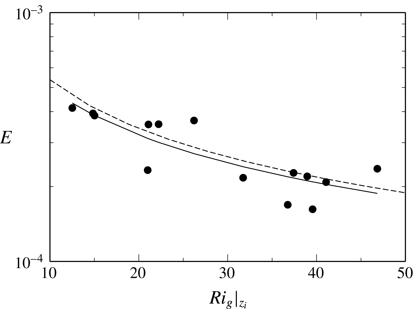
) indicate entrainment is via Holmboe waves, the occurrence and development of which is related to the stability properties of the interface, as indicated by the gradient Richardson number. In figure 13 we plot our data with
 $Ri_{g}|_{z_{i}}$
. Using the empirical fit to the data of Strang & Fernando (Reference Strang and Fernando2001)
 $Ri_{g}=0.038Ri_{b}^{2.0}$
and their result of
 $E=0.0023Ri_{b}^{-1.3}$
we obtain
 $E\simeq 0.0024Ri_{g}|_{z_{i}}^{-0.65}$
. The comparison of this inferred result is close to the regression fit to our data of
 $E=0.0021Ri_{g}|_{z_{i}}^{-0.63}$
. We note that Strang & Fernando (Reference Strang and Fernando2001) report measurements over
 $Ri_{g}<10$
whereas our results extend to
 $Ri_{g}|_{z_{i}}\simeq 50$
and lower values of
 $E$
, but the correlation for both sets of data appears consistent.
The cavity flow considered here then has the same entrainment characteristics as seen in the temporally developing water channel flow when compared using local characteristics, which indicate the state of development of the flow more accurately than the bulk quantities.
Entrainment with gradient Richardson number at the centre of the interface
 $Ri_{g}|_{z_{i}}$
. A regression fit of
 $E=a(Ri_{g}|_{z_{i}})^{b}$
with
 $a=0.0021$
and
 $b=-0.63$
is given (solid line) together with
 $a=0.0024$
and
 $b=-0.65$
(dashed line) derived from the data of Strang & Fernando (Reference Strang and Fernando2001).

4.4 Higher Reynolds number and Richardson number
Finally we consider the possible extension of the entrainment regime we have observed to higher Richardson number. With increasing interface stability, entrainment by molecular diffusion increasingly dominates total mass transport over shear-induced turbulent interfacial mixing (Narimousa et al.
Reference Narimousa, Long and Kitaigorodskii1986; Narimousa & Fernando Reference Narimousa and Fernando1987). We can quantify the molecular entrainment present in our experiments by inspection of the density gradients. The molecular flux of salinity through the interface is given by
 $q_{i}=\unicode[STIX]{x1D705}\text{d}\unicode[STIX]{x1D70C}/\text{d}z=(\unicode[STIX]{x1D708}/Sc)(\unicode[STIX]{x0394}\unicode[STIX]{x1D70C}_{0}/\unicode[STIX]{x1D6FF}_{b})~\text{kg}~\text{m}^{-2}~\text{s}^{-1}$
. For the experiments performed,
 $Sc\simeq 700$
and
 $\unicode[STIX]{x1D708}\simeq 10^{-6}~\text{m}^{2}~\text{s}^{-1}$
. The flux can be written in terms of an entrainment coefficient as
 $q_{i}=u_{e}\unicode[STIX]{x0394}\unicode[STIX]{x1D70C}=E_{m}U_{b}\unicode[STIX]{x0394}\unicode[STIX]{x1D70C}_{0}$
. Combining the relationships we obtain
 $$\begin{eqnarray}E_{m}=\frac{1}{ScRe_{\unicode[STIX]{x1D6FF}}},\end{eqnarray}$$
where
 $Re_{\unicode[STIX]{x1D6FF}}=\unicode[STIX]{x1D6FF}_{b}U_{b}/\unicode[STIX]{x1D708}$
. For our
 $Re=7100$
experiments we obtain
 $Re_{\unicode[STIX]{x1D6FF}}\simeq 70$
and
 $E_{m}=2\times 10^{-5}$
. The lowest entrainment rate measured in our
 $Re=7100$
experiments was
 $E=10^{-4}$
at
 $Ri_{b}=10$
. The ratio of total entrainment
 $E$
to entrainment resulting from molecular diffusion
 $E/E_{m}=5$
indicates that our measurements approach a regime where the total entrainment rate is comparable to molecular diffusion.
Salehipour et al. (Reference Salehipour, Caulfield and Peltier2016) performed direct numerical simulations of the development of the Holmboe wave instability in a periodic domain and identified substantial variation in mixing behaviour with Reynolds number over
 $Re_{\unicode[STIX]{x1D6FF}}=200$
to 12 000. At higher Reynolds number the authors observed the formation of secondary instabilities at the interface, the growth of which is Reynolds-number-dependent up until a critical Reynolds number of
 $Re_{\unicode[STIX]{x1D6FF}}\simeq 8000$
. At high
 $Re$
the authors further observed vigorous long-lived turbulence at the interface which acts to both scour and transport fluid away from the interface and irreversibly mix the fluid. At lower
 $Re$
, mixing was shown to scale with the molecular diffusion rate, and weak ‘wisps’ of fluid on either side of the interface were observed, similar to the flow seen in the present study, as shown in figure 6. In our experiments, there is additional forcing of the interface by turbulence in the overflow, and there is a larger range of wavelengths present in our channel. Neither of these features appear to change this basic low-
 $Re$
mixing characteristic of the flow. Despite the relatively large Reynolds number in the overflow, up to
 $Re=15\,000$
in this study, the shear at the interface remains sufficiently weak that Reynolds numbers at the interface are in the weakly turbulent regime identified by Salehipour et al. (Reference Salehipour, Caulfield and Peltier2016). The extension of this work to environmental scale occurrence of this flow in river systems where
 $Re>10^{5}$
,
 $Sc=700$
and
 $Ri_{b}=10$
to 150 remains a challenge.
5 Conclusions
Entrainment across a sheared interface has been examined experimentally for the case where the interface lies within a shallow cavity with gently sloping entry and exit walls. Using a parametric study we have shown that the flow entrainment mechanisms responsible for purging of dense fluid from the cavity are not the cavity-specific mechanisms that have been encountered in most previous cavity experiments. We have found that entrainment is related to the bulk Richardson number with the scaling
 $E=CRi_{b}^{-1.38}$
, very close to the Richardson number dependence observed by Strang & Fernando (Reference Strang and Fernando2001), Christodoulou (Reference Christodoulou1986) and the data of Deardorff & Willis (Reference Deardorff and Willis1982). Here the length scale is the mixed layer depth and the velocity scale is the bulk velocity in the mixed layer, which, for this configuration, is characteristic of the velocity rise across the interface. We do not observe significant sensitivity of the entrainment rate scaling to Reynolds number across the range
 $Re=7100$
to 15 100 tested in this study. Furthermore we observe no sensitivity to
 $D/H$
other than via the definition of the Richardson number.
Flow visualisations from
 $Ri_{b}=2$
to
 $Ri_{b}=10$
show Holmboe waves and suggest that entrainment occurs as a result of intermittent wave breaking and streamer ejection. The interface is characterised by large amplitude waves with size of the order of the shear layer thickness, while the interface thickness is
 $\unicode[STIX]{x1D6FF}_{b}\sim \unicode[STIX]{x1D6FF}_{s}/10$
. These results, together with the entrainment rate scaling, suggest that the flow is in a regime where entrainment is characterised by breaking Holmboe waves, but in our case the regime extends to a low bulk Richardson number of
 $Ri_{b}=1$
compared with
 $Ri_{b}=5$
observed by Strang & Fernando (Reference Strang and Fernando2001).
In the present configuration the upstream limit of the mixing layer is continually renewed by saline fluid from the cavity. The
 $\unicode[STIX]{x1D6FF}_{b}\simeq 0$
upstream ‘boundary condition’ present in this flow stabilises the entire cavity interface for
 $Ri_{b}>1$
. We have found that the overall magnitude of the entrainment is approximately one order of magnitude smaller than reported by Strang & Fernando (Reference Strang and Fernando2001) in their re-circulating water channel setting, for the same bulk Richardson number, and further suggest that this is a result of this interface stabilisation. When correlated with the local interface scales via the gradient Richardson number we find
 $E=0.0021Ri_{g}|_{z_{i}}^{-0.63}$
over
 $Ri_{g}|_{z_{i}}=10$
to 50, which is very close to the data of Strang & Fernando (Reference Strang and Fernando2001), albeit for conditions at
 $Ri_{g}<10$
. Our results are then an extension of the same flow regime to more stable, higher-
 $Ri_{g}$
conditions. Our measurements show this entrainment regime extends down to the region where transport by molecular diffusion dominates.
The entrainment is controlled via the stability of the interface, which for our flow is strongly related to the initial mixing layer thickness. At very large cavity length, the mixing layer thickness may be expected to approach conditions comparable to the temporally evolving flow of Strang & Fernando (Reference Strang and Fernando2001) and then achieve the same scaling of entrainment with
 $Ri_{b}$
. The development length required to achieve this remains an open question. We have found that the entrainment rate is insensitive to the length of the interface over the experimental range of
 $L/D=2.4$
to 16. The slow adjustment of the interface to bulk conditions is suggested to be due in part to the very low mixing associated with the Holmboe wave regime (Carpenter et al.
Reference Carpenter, Lawrence and Smyth2007). It is possible that these effects may be less prominent at higher
 $Re$
, where increased mixing occurs (Salehipour et al.
Reference Salehipour, Caulfield and Peltier2016); however, more work is needed to answer this question.
The description of an environmental scale occurrence of this flow remains a challenge. While
 $Ri_{b}$
is the only practical measure with which flow conditions may be correlated easily, the scaling
 $E=CRi_{b}^{-1.38}$
does not provide a unique description of entrainment, as the constant of proportionality
 $C$
will vary. We have shown that this variation is up to an order of magnitude, and that the length over which the initial mixing layer thickness affects flow development may be substantial.
Acknowledgements
The authors acknowledge the support of the Australian Research Council under grant DP110103417.
Supplementary movie
A supplementary movie is available at https://doi.org/10.1017/jfm.2017.796.