





Introduction
In-band full-duplex system (IBFD) is one of the potential candidates for next 6G wireless communication system, where circulators are used for isolating transmitting and receiving paths of IBFD radio frequency (RF) front-end [Reference Kolodziej, Perry and Herd1]. Therefore, nonreciprocal circuits such as circulators and isolators are crucial components in communication systems, IBFD, radar, and in protecting power amplifiers from undesired reflections due to their ability to allow unidirectional signal propagation [Reference Hong, Brand, Choi, Jain, Mehlman and Katti2, Reference Park, Myeong, Rebeiz and Kim3]. Traditionally, circulators and isolators are designed by possessing an asymmetric permeability tensor of ferrite magnetic materials [Reference Oliver4–Reference Ghadiya, Trivedi, Son and Bhatt9]. Ferrite-based circulators and isolators are widely used due to their low insertion loss (IL) and high-power handling capability. However, these ferrite-based circulators and isolators suffer from several drawbacks, including bulky size, high cost, and incompatibility with integrated circuit (IC) technologies. To eliminate the use of ferrite materials, circulators and isolators are designed using transistors and nonlinear active devices [Reference Tanaka, Shimomura and Ohtake10–Reference Mung and Chan12] with the goal of achieving integration with IC technologies. However, these active transistor-based circulators and isolators often suffer from poor noise figure and limited power handling capability.
In recent years, both industrial and academic communities have focused on developing ferrite-free circulators/isolators that are compatible with IC technologies by using linear periodically time-varying (LPTV) circuits [Reference Reiskarimian, Nagulu, Dinc and Krishnaswamy13, Reference Reiskarimian, Zhou and Krishnaswamy14]. These LPTV circuits introduce temporal modulation to break Lorentz nonreciprocity without the use of any magnetic materials. For instance, in paper [Reference Reiskarimian and Krishnaswamy15], a magnetless circulator is developed by incorporating 180° phase shifted gyrator-based N-path filter within 3λ/4 transmission lines (TLs). The fabricated N-path filter-based circulator has achieved forward transmission IL of 3.3 dB and reverse isolation (IX) of 17.4 dB at a center frequency of 750 MHz and 20-dB isolation fractional bandwidth (FBWIX) of 4.3% (32 MHz) at 750 MHz. In subsequent work [Reference Dinc, Tymchenko, Nagulu, Sounas, Alú and Krishnaswamy16], the reverse isolation bandwidth of such circulators is improved by sequentially switching a pair of balanced λ/4 delay lines.
Similarly, magnetless circulators are also developed based on angular-momentum biasing, in the form of spatiotemporal modulation (STM) by continuously modulating the permittivity of a ring of resonators [Reference Estep, Sounas and Alu17]. In subsequent works [Reference Estep, Sounas, Soric and Alu18–Reference Kord, Tymchenko, Sounas, Krishnaswamy and Alu22], discrete implementations of magnet-free circulators are demonstrated by spatiotemporally modulating the oscillation frequencies of the three lumped-LC resonators, providing high reverse isolation with a FBWIX of 3.8%. Other approaches use bandpass film bulk acoustic resonators [Reference Torunbalci, Odelberg, Sridaran, Ruby and Bhave23], bandpass MEMS resonators [Reference Xu and Piazza24], and bandstop resonators [Reference Kord, Sounas and Alu25] to design STM-based circulators. While these designs demonstrate strong nonreciprocity, STM-based magnetless circulators face several challenges, including high transmission IL, narrow isolation bandwidth, and poor in-band impedance matching. Recently, microstrip line circulators utilizing static and time-modulated resonators have been demonstrated in paper [Reference Wu and Liu26]; however, frequency response is not tunable.
To address these limitations, this paper proposes a frequency-tunable magnetless circulator based on mixed static and time-modulated resonators. This paper is an extension of work [Reference Chaudhary, Thorng, Kim and Jeong27], where an earlier version of this work was presented at European Microwave Week 2025. In previous works [Reference Estep, Sounas, Soric and Alu18–Reference Kadry, Alhawari and Sounas21, Reference Torunbalci, Odelberg, Sridaran, Ruby and Bhave23, Reference Xu and Piazza24, Reference Chaudhary, Thorng, Kim and Jeong27], the behavior of circulators is analyzed by using the harmonic balance (HB) method. However, the HB method suffers from convergence issues and high computational complexity. In this extended study, a detailed comprehensive analysis of the proposed circulator is carried out using analytically derived spectral S-parameters, without relying on HB simulations. To provide insight into the nonreciprocity phenomenon, the spectral admittance matrices of both static and time-modulated resonators are derived. These spectral admittance matrices enable the interpretation of time-invariant and time-variant circuit elements in the full spectral domain. Furthermore, to analyze the cause of IL under practical conditions, unloaded quality factors (Q-factors) of the static and time-modulated resonators are incorporated into the spectral admittance matrices. Numerical results show that the proposed circulator exhibits excellent frequency-tunable filtering performance, including improved passband transmission flatness and suppressed first intermodulation (IM) product signal power, enhanced stopband suppression, high reverse isolation bandwidth, and good port impedance matching.
Theoretical analysis and design method
Figure 1(a) shows the circuit diagram of previously reported STM-based circulators [Reference Estep, Sounas and Alu17, Reference Estep, Sounas, Soric and Alu18] consisting of one time-modulated resonator at each branch. These conventional circulators exhibit high forward transmission IL, poor passband transmission flatness, and single null isolation characteristics as depicted in the figure. Figure 1(b) shows the circuit diagram of the proposed frequency-tunable circulator, which consists of static and time-modulated resonators at each branch. In each branch, ports are coupled to static resonators ( $Z_{LC1}^{\left( i \right)}$) through impedance inverter K 01, whereas static resonators are coupled to time-modulated resonators (
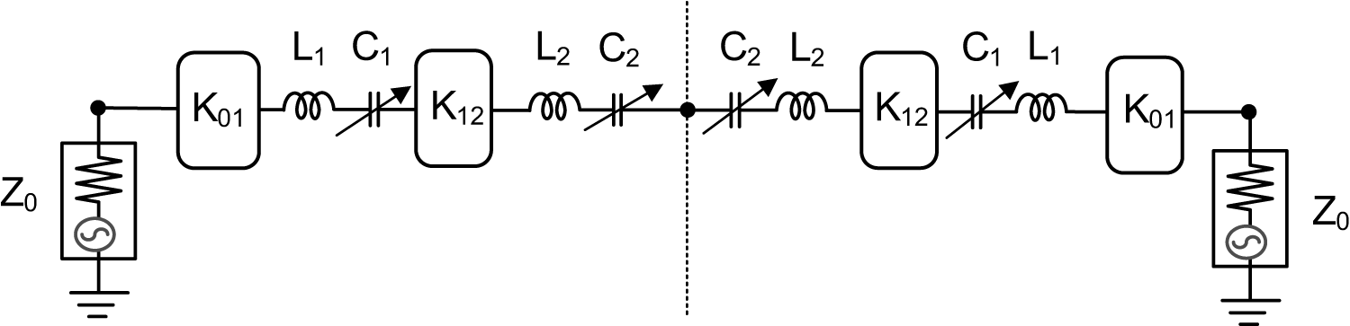
 $Z_{LC2}^{\left( i \right)}$) through impedance inverter K 12. The admittance inverter values can be extracted from the equivalent two-port third-order bandpass filter of the two branches, as shown in Figure2. The values of admittance inverters can be found as (1) using third-order low-pass filter prototype element values (i.e. g 0, g 1, g 2, g 3, …).
 \begin{equation}{K_{01}} = \sqrt {\frac{{{A_0} \times B{W_{static}}}}{{2\pi f_0^2{g_0}{g_1}{C_1}}}} .\end{equation}
 \begin{equation}{\text{ }}{K_{12}} = \frac{{B{W_{static}}}}{{2\pi f_0^2\sqrt {{g_1}{g_2}{C_1}{C_2}} }},\end{equation}
Circuit diagram and conceptual frequency response of magnetless circulators using spatiotemporal modulation techniques: (a) conventional circulator [Reference Estep, Sounas and Alu17, Reference Estep, Sounas, Soric and Alu18], and (b) proposed circulator using mixed static and time-modulated resonators.

Equivalent circuit of two branches, which is equivalent to a two-port third-order bandpass filter.

where A 0 is an arbitrary positive value, and BWstatic is the bandwidth of the circulator at static state (without modulation).
Analysis of static and time-modulated resonators
To achieve nonreciprocity, the self-capacitance of time-modulated resonators (i.e.  $C_2^{\left( 1 \right)}\left( t \right),\,\,C_2^{\left( 2 \right)}\left( t \right),\,$and
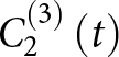 $\,C_2^{\left( 3 \right)}\left( t \right)$) is spatiotemporally modulated by sinusoidal waves with a progressive phase shift of ∆φ as given in (2).
 \begin{equation}C_2^{(i)}\left( t \right) = {C_2}\left\{ {1 + m\sin \left( {2\pi {f_m}t + \left( {i - 1} \right)\Delta \varphi } \right)} \right\},\end{equation}
where i (= 1, 2, 3) corresponds to three branches and C 2 is the nominal capacitance (without modulation), m is modulation index, and fm is the modulation frequency [Reference Wu, Liu, Hickle, Peroulis, Gómez-díaz and Melcon28]. To realize nonreciprocal circulator operation using the STM technique [Reference Estep, Sounas and Alu17, Reference Estep, Sounas, Soric and Alu18], the progressive phase shift of the sinusoidal modulation signal must be set to ∆φ = 120o.
For the purpose of analytical synthesis of time-modulated resonators, a spectral matrix W is defined as (3) by assuming N har (i.e.  $(k = {\text{ }} - {N_{har}},\,\, \cdots , - 2,{\text{ }} - 1,{\text{ }}0,{\text{ }} + 1,{\text{ }} + 2,\, \cdots \,,{N_{har}})$ to capture all the spectra inside the time-modulated resonators [Reference Wu, Liu, Hickle, Peroulis, Gómez-díaz and Melcon28].
 \begin{equation}\begin{gathered}
{\textbf{ }}\begin{array}{*{20}{c}}
{{\text{ }}{k_1}}&{ - 2}&{ - 1}&0&{ + 1}&{ + 2}& \cdots &{{k_2}}
\end{array} \hfill \\
{\textbf{W}} = \left[ {\begin{array}{*{20}{c}}
\ddots & \cdots & \cdots & \cdots & \cdots & {{{.}}}\mkern2mu
\text{.} \\
0& {{x^{ - 2}}} &0&0&0&0& \cdots \\
\cdots &0&{{x^{ - 1}}}&0&0&0& \cdots \\
\cdots &0&0& {{x^0}}&0&0& \cdots \\
\cdots &0&0&0&{{x^{ + 1}}}&0& \cdots \\
\cdots &0&0&0&0& {{x^{ + 2}}}& \vdots \\
{{{.}}}\mkern2mu
\text{.} & \vdots & \vdots & \vdots & \vdots &0& \ddots
\end{array}} \right]\begin{array}{*{20}{c}}
\vdots \\
{ - 2} \\
{ - 1} \\
0 \\
{ + 1} \\
{ + 2} \\
\vdots
\end{array}, \hfill \\
\end{gathered} \end{equation}
 \begin{equation}{x^k} = 2\pi \left( {f - k{f_m}} \right),{\text{ }}k \in \left\{ { - {N_{har}}, \cdots , - 2, - 1,0,1,2, \cdots ,{N_{har}}} \right\},\end{equation}
where f is the RF carrier frequency and fm is the modulation frequency. In (3a), the diagonal elements (i.e. xk) are non-zero while other elements are zero. The diagonal elements correspond to the fundamental and harmonic frequencies, as given in (3b). Using the spectral matrix W, the spectral impedance  ${\boldsymbol{Z}}_{\boldsymbol{C}}^{\left( {\boldsymbol{i}} \right)}$ of the time-modulated capacitor
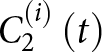 $C_2^{\left( i \right)}\left( t \right)$ defined in (2) can be rewritten as (4).
 \begin{align}Z_{c2}^{(i)}&=\frac1{jC_2}\times\begin{bmatrix}\ddots&\vdots&\vdots&\vdots&\vdots&\vdots&\vdots\\\dots&\frac1{x^{-2}}&\frac{mA}{2x^{-2}}&0&0&0&\dots\\0&\frac{mB}{2x^{+1}}&\frac1{x^{-1}}&\frac{mA}{2x^{-1}}&0&0&\dots\\0&0&\frac{mB}{2x^0}&\frac1{x^0}&\frac{mA}{2x^0}&0&\dots\\0&0&0&\frac{mB}{2x^{+1}}&\frac1{x^{+1}}&\frac{mA}{2x^0}&\dots\\\vdots&\vdots&0&0&\frac{mB}{2x^{+2}}&\frac1{x^{+2}}&\dots\\\vdots&\vdots&\vdots&\vdots&0&\vdots&\ddots\end{bmatrix}
\nonumber\\ \quad\quad& A=e^{-j\left(i-1\right)\frac{2\pi}3},B=e^{j\left(i-1\right)\frac{2\pi}3}\end{align}
When the time-varying capacitors given in (1) are transformed into the frequency domain, their spectral impedances contain not only at RF fundamental frequency but also IM products at 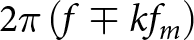 $2\pi \left( {f \mp k{f_m}} \right)$. These components arise due to sinusoidal modulation of the capacitor. Therefore, the diagonal elements (i.e.
 $1/{x^k},k = \, \cdots , - 2, - 1,\,0,\,1,2, \cdots $) in (4) represent the self-impedance of the time-modulated capacitor at each spectral frequency, whereas off-diagonal elements (i.e.
 $m/{x^k}{e^{ \mp j\left( {i - 1} \right)2\pi /3}},\,\,k = \, \cdots , - 2, - 1,\,0,\,1,2, \cdots ,\,i = 1\,,\,2,\,\,3$) are transimpedance, which represents conversion/coupling between a pair of spectral frequencies. To insight full spectra of time-modulated resonators, the spectral admittance matrix can be rewritten as (5), where U is the unitary matrix of the same dimension as W.
 \begin{equation}{\textbf{Z}}_{_{C2}}^{(i)} = - j{{\textbf{W}}^{ - 1}} \times \frac{{{{{\lambda }}^{(i)}}}}{{{C_2}}}.\end{equation}
where the value of the new spectral matrix  $\,{{\boldsymbol{\lambda }}^{\left( {\boldsymbol{i}} \right)}}$ can be defined as (6).
 \begin{align}\lambda^{(i)}&=U-\frac12\begin{bmatrix}\ddots&\vdots&\vdots&\vdots&\vdots&\vdots&\vdots\\\dots&0&mA&0&0&0&\dots\\0&mB&0&mA&0&0&\dots\\0&0&mB&0&mA&0&\dots\\0&0&0&mB&0&mA&\dots\\\vdots&\vdots&0&0&mB&0&\dots\\\vdots&\vdots&\vdots&\vdots&0&\vdots&\ddots\end{bmatrix} \nonumber\\
& A=e^{j(i-1)\frac{2\pi}3},B=e^{-j(i-1)\frac{2\pi}3}\end{align}
When λ(i) reduces to a unitary matrix in the absence of modulation (i.e. m = 0), the impedance of the time-modulated capacitor given in (5) reduces to that of a static capacitor case. However, when the capacitor is modulated, the off-diagonal elements (i.e.  $m/{x^k}{e^{ \mp j\left( {i - 1} \right)2\pi /3}},$
 $k\, = \, \cdots , - 2, - 1,\,0,\,1,2, \cdots ,\,i = 1,2,3$) of
 ${\boldsymbol{Z}}_{{\boldsymbol{c}}2}^{\left( {\boldsymbol{i}} \right)}$ acquire complex terms of equal magnitude but opposite phase with respect to the diagonal reference. As a result,
 ${\boldsymbol{Z}}_{{\boldsymbol{c}}2}^{\left( {\boldsymbol{i}} \right)}$ contains both time-invariant and time-variant element values across the full spectral domain. This provides a physically intuitive interpretation of nonreciprocal behavior. The time-varying elements introduce phase-dependent terms in (5) and (6), which can create phase-dependent nonreciprocity between adjacent terms. When several such nonreciprocal elements are cascaded, the nonreciprocal transmission at the carrier frequency occurs due to the conversion and interaction between two distinct spectral components.
Using (3)–(6), the spectral admittance matrices of static and time-modulated resonators can be derived as (7).
 \begin{equation}{\textrm Z}_{LC1}^{\left( i \right)} = j\left\{ {{\textbf{W}}{L_1} - \frac{{{{\textbf{W}}^{ - 1}}}}{{{C_1}}}} \right\}\end{equation}
 \begin{equation}{\textrm Z}_{LC2}^{\left( i \right)} = j\left\{ {{\textbf{W}}{L_2} - {{\textbf{W}}^{ - 1}} \times \frac{{{{{\lambda }}^{(i)}}}}{{{C_2}}}} \right\},\end{equation}
where L 1 and L 2 represent the inductance of the static and time-modulated resonators, respectively. For each resonator, the value of the inductor can be calculated using  ${L_i} = 1/4{\pi ^2}f_0^2{C_i}$, where
 ${f_0}$ is the RF carrier center frequency. In (7), the spectral admittances of the static and time-modulated resonators are assumed to be lossless. However, in practice, perfectly lossless resonators are not realizable. Therefore, by considering unloaded Q-factors of the static and time-modulated resonators as
 $Q_u^s$ and
 $Q_u^m$ respectively, the spectral admittance matrix can be rewritten as (8), where U is a unitary matrix.
 \begin{equation}{\textrm Z}_{LC1}^{\left( i \right)} = {\textbf{W}} \times \frac{{{L_1}}}{{Q_u^s}} + j\left\{ {{\textbf{W}}{L_1} - \frac{{{{\textbf{W}}^{ - 1}}}}{{{C_1}}}} \right\}\end{equation}
 \begin{equation}{\textrm Z}_{LC2}^{\left( i \right)} = {\textbf{W}} \times \frac{{{L_2}}}{{Q_u^m}} + j\left\{ {{\textbf{W}}{L_2} - {{\textbf{W}}^{ - 1}} \times \frac{{{{{\lambda }}^{(i)}}}}{{{C_2}}}} \right\},\end{equation}
When  $Q_u^s$ and
 $Q_u^m$ approach infinity, the spectral impedances reduce to those in (7).
Spectral S-parameters of the proposed circulator
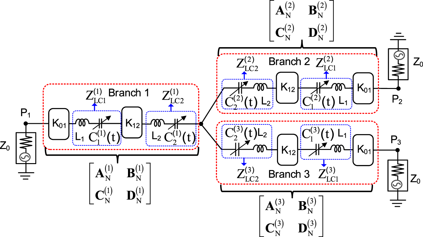
As seen from Figure 1(b), the proposed circulator consists of three branches, forming a Y-network by connecting branches at a common junction. The spectral total ABCD-matrix of each branch can be computed using (9), as illustrated in Figure 3.
 \begin{equation}\left[ {\begin{array}{*{20}{c}}
{{\textbf{A}}_N^{(1)}}&{{\textbf{B}}_N^{(1)}} \\
{{\textbf{C}}_N^{(1)}}&{{\textbf{D}}_N^{(1)}}
\end{array}} \right] = {{\textbf{N}}_a} \times {{\textbf{N}}_b} \times {{\textbf{N}}_c} \times {{\textbf{N}}_d}\end{equation}
 \begin{equation}\left[ {\begin{array}{*{20}{c}}
{{\textbf{A}}_N^{(2)}}&{{\textbf{B}}_N^{(2)}} \\
{{\textbf{C}}_N^{(2)}}&{{\textbf{D}}_N^{(2)}}
\end{array}} \right] = {{\textbf{M}}_a} \times {{\textbf{M}}_b} \times {{\textbf{M}}_c} \times {{\textbf{M}}_d}\end{equation}
 \begin{equation}\left[ {\begin{array}{*{20}{c}}
{{\textbf{A}}_N^{(3)}}&{{\textbf{B}}_N^{(3)}} \\
{{\textbf{C}}_N^{(3)}}&{{\textbf{D}}_N^{(3)}}
\end{array}} \right] = {{\textbf{T}}_a} \times {{\textbf{T}}_b} \times {{\textbf{T}}_c} \times {{\textbf{T}}_d},\end{equation}
Procedure for computing the spectral ABCD-parameters of each-branch.

where
 \begin{align}{{\textbf{N}}_a}& = {{\textbf{M}}_d} = {{\textbf{T}}_d} = \left[ {\begin{array}{*{20}{c}}
0&{{K_{01}}{\textbf{U}}} \\
{\frac{{\textbf{U}}}{{{K_{01}}}}}&0
\end{array}} \right],{\text{ }}\nonumber\\ {{\textbf{N}}_c} &= {{\textbf{M}}_b} = {{\textbf{T}}_b} = \left[ {\begin{array}{*{20}{c}}
0&{{K_{12}}{\textbf{U}}} \\
{\frac{{\textbf{U}}}{{{K_{12}}}}}&0
\end{array}} \right]\end{align}
 \begin{equation}{{\textbf{N}}_b} = \left[ {\begin{array}{*{20}{c}}
{\textbf{U}}&{{\textbf{Z}}_{LC1}^{(1)}} \\
0&{\textbf{U}}
\end{array}} \right],{{\textbf{N}}_d} = \left[ {\begin{array}{*{20}{c}}
{\textbf{U}}&{{\textbf{Z}}_{LC2}^{(1)}} \\
0&{\textbf{U}}
\end{array}} \right]\end{equation}
 \begin{equation}{{\textbf{M}}_a} = \left[ {\begin{array}{*{20}{c}}
{\textbf{U}}&{{\textbf{Z}}_{LC2}^{(2)}} \\
0&{\textbf{U}}
\end{array}} \right],{{\textbf{T}}_a} = \left[ {\begin{array}{*{20}{c}}
{\textbf{U}}&{{\textbf{Z}}_{LC2}^{(3)}} \\
0&{\textbf{U}}
\end{array}} \right]\end{equation}
 \begin{equation}{{\textbf{M}}_c} = \left[ {\begin{array}{*{20}{c}}
{\textbf{U}}&{{\textbf{Z}}_{LC1}^{(2)}} \\
0&{\textbf{U}}
\end{array}} \right],{{\textbf{T}}_c} = \left[ {\begin{array}{*{20}{c}}
{\textbf{U}}&{{\textbf{Z}}_{LC1}^{(3)}} \\
0&{\textbf{U}}
\end{array}} \right].\end{equation}
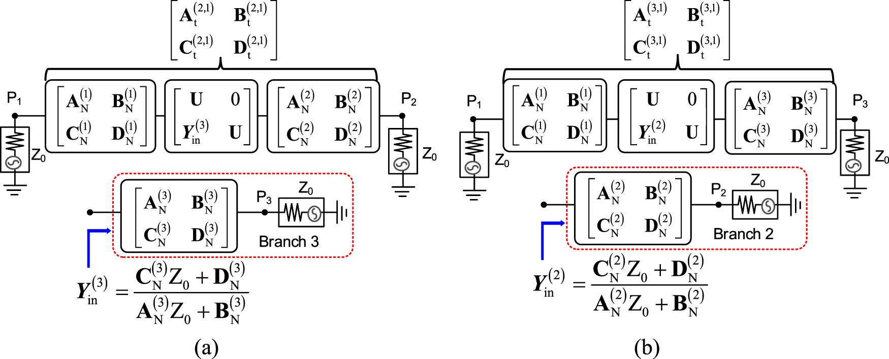
Assuming branch 3, including port impedance Z 0 = 50 Ω as a shunt susceptance element shown in Figure 4(a), the total spectral ABCD-parameters between ports 2 and 1 can be derived as (11).
 \begin{align}\left[ {\begin{array}{*{20}{c}}
{{\textbf{A}}_t^{(2,1)}}&{{\textbf{B}}_t^{(2,1)}} \\
{{\textbf{C}}_t^{(2,1)}}&{{\textbf{D}}_t^{(2,1)}}
\end{array}} \right]& = \left[ {\begin{array}{*{20}{c}}
{{\textbf{A}}_N^{(1)}}&{{\textbf{B}}_N^{(1)}} \\
{{\textbf{C}}_N^{(1)}}&{{\textbf{D}}_N^{(1)}}
\end{array}} \right] \times \left[ {\begin{array}{*{20}{c}}
{\textbf{U}}&0 \\
{{\boldsymbol{Y}}_{in}^{(3)}}&{\textbf{U}}
\end{array}} \right] \nonumber\\ &\quad{}\times \left[ {\begin{array}{*{20}{c}}
{{\textbf{A}}_N^{(2)}}&{{\textbf{B}}_N^{(2)}} \\
{{\textbf{C}}_N^{(2)}}&{{\textbf{D}}_N^{(2)}}
\end{array}} \right],\end{align}
Procedure for computing total spectral ABCD-parameters of the proposed circulator: (a) between ports 2 and 1, and (b) between ports 3 and 1.

where
 \begin{equation}{\boldsymbol{Y}}_{in}^{(3)} = \frac{{{\textbf{C}}_N^{(3)}{Z_0} + {\textbf{D}}_N^{(3)}}}{{{\textbf{A}}_N^{(3)}{Z_0} + {\textbf{B}}_N^{(3)}}}.\end{equation}
In a similar manner, as illustrated in Figure 4(b), the total spectral ABCD-parameters between ports 1 and 3 can be determined as (13).
 \begin{align}\left[ {\begin{array}{*{20}{c}}
{{\textbf{A}}_t^{(3,1)}}&{{\textbf{B}}_t^{(3,1)}} \\
{{\textbf{C}}_t^{(3,1)}}&{{\textbf{D}}_t^{(3,1)}}
\end{array}} \right] & = \left[ {\begin{array}{*{20}{c}}
{{\textbf{A}}_N^{(1)}}&{{\textbf{B}}_N^{(1)}} \\
{{\textbf{C}}_N^{(1)}}&{{\textbf{D}}_N^{(1)}}
\end{array}} \right] \times \left[ {\begin{array}{*{20}{c}}
{\textbf{U}}&0 \\
{{\boldsymbol{Y}}_{in}^{(2)}}&{\textbf{U}}
\end{array}} \right]\nonumber\\&\quad{} \times \left[ {\begin{array}{*{20}{c}}
{{\textbf{A}}_N^{(3)}}&{{\textbf{B}}_N^{(3)}} \\
{{\textbf{C}}_N^{(3)}}&{{\textbf{D}}_N^{(3)}}
\end{array}} \right],\end{align}
where
 \begin{equation}{\boldsymbol{Y}}_{in}^{(2)} = \frac{{{\textbf{C}}_N^{(2)}{Z_0} + {\textbf{D}}_N^{(2)}}}{{{\textbf{A}}_N^{(2)}{Z_0} + {\textbf{B}}_N^{(2)}}}.\end{equation}
After obtaining the total spectral ABCD-parameters between ports 2 and 1, and ports 3 and 1, as illustrated in Figure 4, the spectral S-parameters can be computed using the spectral ABCD-parameters to spectral S-parameters conversion relation [Reference Wu, Liu, Hickle, Peroulis, Gómez-díaz and Melcon28], as given in (15).
 \begin{equation}{\boldsymbol{S}}_{11}^{\left( {{k_1},{k_2}} \right)} = {\textbf{U}} - \frac{{2{Z_0}\left( {{\textbf{C}}_t^{(2,1)} + {\textbf{D}}_t^{(2,1)}} \right)}}{{{\textbf{A}}_t^{(2,1)}{Z_0} + {\textbf{B}}_t^{(2,1)} + {\textbf{C}}_t^{(2,1)}Z_0^2 + {\textbf{D}}_t^{(2,1)}{Z_0}}}\end{equation}
 \begin{equation}{\boldsymbol{S}}_{22}^{\left( {{k_1},{k_2}} \right)} = {\textbf{U}} - \frac{{2{\textbf{U}}}}{{{\textbf{U}} + {{\left( {{\textbf{A}}_t^{(2,1)}{Z_0} + {\textbf{C}}_t^{(2,1)}Z_0^2} \right)}^{ - 1}}\left( {{\textbf{B}}_t^{(2,1)} + {\textbf{D}}_t^{(2,1)}{Z_0}} \right)}}\end{equation}
 \begin{equation}{\boldsymbol{S}}_{33}^{\left( {{k_1},{k_2}} \right)} = {\textbf{U}} - \frac{{2{\textbf{U}}}}{{{\textbf{U}} + {{\left( {{\textbf{A}}_t^{(3,1)}{Z_0} + {\textbf{C}}_t^{(3,1)}Z_0^2} \right)}^{ - 1}}\left( {{\textbf{B}}_t^{(3,1)} + {\textbf{D}}_t^{(3,1)}{Z_0}} \right)}}\end{equation}
 \begin{equation}{\boldsymbol{S}}_{21}^{\left( {{k_1},{k_2}} \right)} = \frac{{2{Z_0}{\textbf{U}}}}{{{\textbf{A}}_t^{(2,1)}{Z_0} + {\textbf{B}}_t^{(2,1)} + {\textbf{C}}_t^{(2,1)}Z_0^2 + {\textbf{D}}_t^{(2,1)}{Z_0}}}\end{equation}
 \begin{equation}{\boldsymbol{S}}_{12}^{\left( {{k_1},{k_2}} \right)} = \left\{ \begin{gathered}
2 \bigg[ U + \left( {{\textbf{A}}_t^{(2,1)}{Z_0} + {\textbf{B}}_t^{(2,1)}} \right)\hfill \\ \times {{{{\left( {{\textbf{C}}_T^{(2,1)}{Z_0} + {\textbf{D}}_t^{(2,1)}} \right)}^{ - 1}}} \mathord{\left/
{\vphantom {{{{\left( {{\textbf{C}}_T^{(2,1)}{Z_0} + {\textbf{D}}_t^{(2,1)}} \right)}^{ - 1}}} {{Z_0}}}} \right.
} {{Z_0}}} \bigg]^{ - 1} \hfill \\
\times \left[ {\textbf{A}}_t^{(2,1)} - \left( {{\textbf{A}}_t^{(2,1)}{Z_0} + {\textbf{B}}_t^{(2,1)}} \right)\right. \hfill\\ \times \left.{{\left( {{\textbf{C}}_t^{(2,1)}{Z_0} + {\textbf{D}}_t^{(2,1)}} \right)}^{ - 1}} {\textbf{C}}_t^{(2,1)} \right] \hfill \\
\end{gathered} \right\}\end{equation}
 \begin{equation}{\boldsymbol{S}}_{31}^{\left( {{k_1},{k_2}} \right)} = \frac{{2{Z_0}{\textbf{U}}}}{{{\textbf{A}}_t^{(3,1)}{Z_0} + {\textbf{B}}_t^{(3,1)} + {\textbf{C}}_t^{(3,1)}Z_0^2 + {\textbf{D}}_t^{(3,1)}{Z_0}}}\end{equation}
 \begin{equation}{\boldsymbol{S}}_{13}^{\left( {{k_1},{k_2}} \right)} = \left\{ \begin{gathered}
2\bigg[ U + \left( {{\textbf{A}}_t^{(3,1)}{Z_0} + {\textbf{B}}_t^{(3,1)}} \right)\hfill \\ \times{{{{\left( {{\textbf{C}}_T^{(3,1)}{Z_0} + {\textbf{D}}_t^{(3,1)}} \right)}^{ - 1}}} \mathord{\left/
{\vphantom {{{{\left( {{\textbf{C}}_T^{(3,1)}{Z_0} + {\textbf{D}}_t^{(3,1)}} \right)}^{ - 1}}} {{Z_0}}}} \right.
} {{Z_0}}} \bigg]^{ - 1}\hfill \\
\times \left[ {\textbf{A}}_t^{(3,1)} - \left( {{\textbf{A}}_t^{(3,1)}{Z_0} + {\textbf{B}}_t^{(3,1)}} \right)\right. \hfill\\ \times \left.{{\left( {{\textbf{C}}_t^{(3,1)}{Z_0} + {\textbf{D}}_t^{(3,1)}} \right)}^{ - 1}}{\textbf{C}}_t^{(3,1)} \right] \hfill \\
\end{gathered} \right\}\end{equation}
Since the proposed circuit is symmetrical, the value of 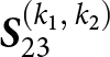 ${\boldsymbol{S}}_{23}^{\left( {{k_1},\,{k_2}} \right)}\,$is equal to
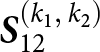 ${\boldsymbol{S}}_{12}^{\left( {{k_1},\,{k_2}} \right)}$ and the value of
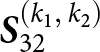 ${\boldsymbol{S}}_{32}^{\left( {{k_1},\,{k_2}} \right)}\,$is equal to
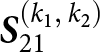 ${\boldsymbol{S}}_{21}^{\left( {{k_1},\,{k_2}} \right)}$, where k 1 and k 2 represent indices of harmonics. Since the spectral S-parameters derived in (15) are represented by matrices of dimensions (2N har + 1) × (2N har + 1), the circulator S-parameters at the fundamental RF frequency (i.e.
 ${S_{i,j}} = {\boldsymbol{S}}_{i,j}^{\left( {0,\,0} \right)}\,,\,i,\,j = 1,\,2,\,3)$ are extracted from the central element, i.e at (2N har + 2)/2 index of the spectral S-parameter matrix.
The procedure for computing the S-parameters based on the above equations can be summarized as follows:
1) Specify values of BW static, RF center frequency (f 0), C 1, C 2, f m, m, and
 $Q_u^m$, and RF carrier frequency (f) range from f 1 to f 2 with an appropriate frequency step. In addition, determine the low-pass filter prototype element values for a third-order static (unmodulated) filter.
2) Compute inductance as
${L_1} = 1/4{\pi ^2}f_0^2{C_1}$,
${L_2} = 1/4{\pi ^2}f_0^2{C_2}$, and coupling coefficients K 01 and K 12 using (1a) and (1b), respectively.3) For each RF carrier frequency, compute the spectral impedances of the static resonators
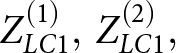
$Z_{LC1}^{\left( 1 \right)},\,Z_{LC1}^{\left( 2 \right)},$ and
$\,Z_{LC1}^{\left( 3 \right)}$ of each branch using (3a), (3b), (6), and (8a). Similarly, calculate the spectral impedance of the time-modulated resonators
$Z_{LC2}^{\left( 1 \right)}$,
$Z_{LC2}^{\left( 2 \right)}$, and
$Z_{LC2}^{\left( 3 \right)}\,$of each branch using (3a), (3b), (6), and (8b).4) Compute the total ABCD-parameters of branches 1–3 using (9) and (10). Once the total spectral ABCD-parameters of each branch are obtained, calculate the values of
$Y_{in}^{\left( 3 \right)}$ and
$Y_{in}^{\left( 2 \right)}$ using (12) and (14), respectively.5) Compute the total spectral ABCD-parameters between ports 2 and 1, and between ports 3 and 1 using (11)–(14).
6) After obtaining the total spectral ABCD-parameters between ports 2 and 1, and ports 3 and 1, calculate the spectral S-parameters using (15) by substituting the corresponding spectral ABCD-parameters of each branch.
7) Extract the circulator S-parameters at the fundamental RF (
${S_{i,j}} = {\boldsymbol{S}}_{i,j}^{\left( {0,\,0} \right)}\,,\,i,\,j = 1,\,2,\,3)$ from the central element, i.e. at (2N har + 2)/2 index of the spectral S-parameter matrix.8) Steps (3)–(7) are repeated for each RF carrier frequency over the specified frequency sweep range defined in step (1).






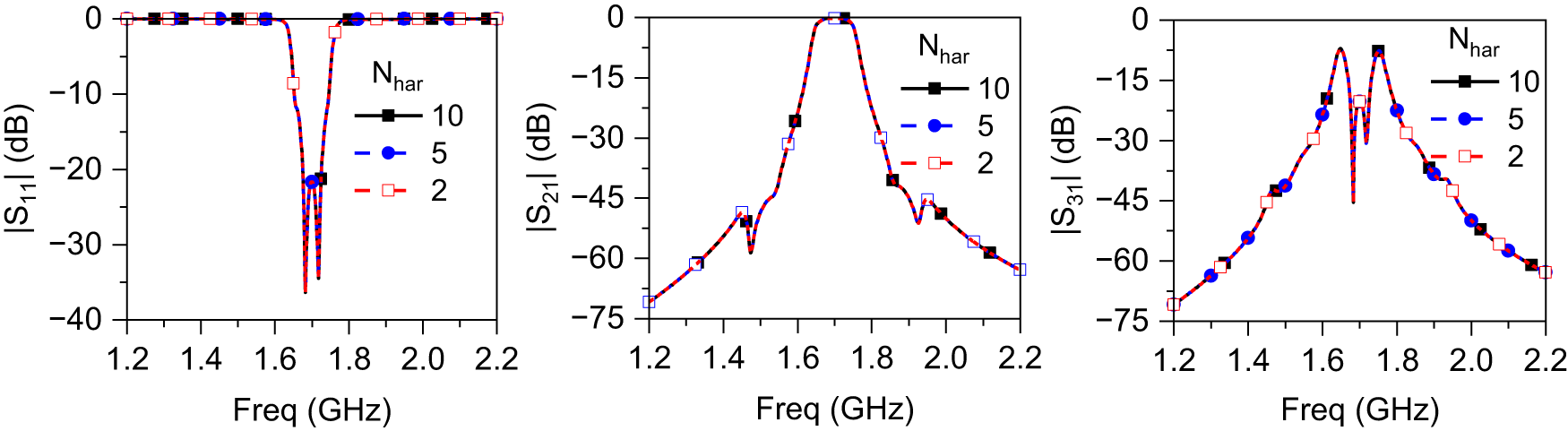
To validate the proposed analytical formulation, Figure 5 illustrates the calculated S-parameters for different values of Nhar. For this case, the circulator is designed to exhibit 0.01 dB-ripple Chebyshev response with a bandwidth of 90 MHz at static state (without modulation). It is observed that the S-parameters are unchanged regardless of the number of harmonics considered. However, increasing Nhar results in larger matrix dimensions and higher computational cost. Therefore, Nhar = 2 is sufficient for accurate S-parameters computation. In addition, the proposed circulator demonstrates filtering characteristics with low transmission IL, two nulls in reverse isolation (IX = |S 21|) characteristic, and two poles in reflection characteristics.
Analytically calculated S-parameters with different N har. Circuit parameters: A 0 = 1, g 0 = 1, g 1 = 0.9146, g 2 = 0.6857, BWstatic = 75 MHz, f 0 = 1.70 GHz, C 1 = C 2 = 6 pF, L 1 = L 2 = 1.4608 nH, with infinite resonator Q-factors. Modulation parameters: fm = 183.75 MHz, m = 0.1513. In this figure, |S 11| = |S 22| = |S 33|, |S 21| = |S 32| = |S 13|, and |S 12| = |S 31| = |S 23|.

To present an intuitive understanding of how the modulation frequency (fm) and modulation index (m) affect the frequency response, Figure 6 shows contour heatmap plots of return loss (|S 11|), transmission IL (IL = |S 21|), and reverse isolation (IX = |S 31|) at an RF carrier center frequency of 1.70 GHz. When modulation frequency f m is between 200 and 230 MHz and modulation index m is in the range of 0.172–0.195, strong IX (>25 dB) is achieved with transmission IL less than 0.40 dB, assuming unloaded Q-factors of static and time-modulated resonators equal to 1000. However, the transmission IL degrades to 3.7 dB when unloaded Q-factors decrease to 80.
Calculated reflection coefficient (i.e. |S 11| = |S 22| = |S 33|), transmission coeffcients i.e. IL = |S 21| = |S 32| = |S 13|) and reverse isolation (i.e. IX = |S 12| = |S 23| = |S 31|) at RF carrier frequency (f 0) of 1.7 GHz according modulation frequency (fm) and modulation index (m). Circuit parameters: A0 = 1, g 0 = 1, g 1 = 0.9146, g 2 = 0.6857, BWstatic = 90 MHz, C 1 = C 2 = 6 pF, L 1 = L 2 = 1.4608 nH.

Similarly, Figures 7 and 8 show contour heatmap plots of reflection coefficient (|S 11|), forward transmission coefficient (|S 21|), and reverse isolation (|S 31|) over the RF carrier frequency range of 1.40–2.0 GHz. These results are obtained numerically for different unloaded Q-factors, modulation frequency fm, and modulation index m. As observed from these results, the higher values of m enable high reverse isolation (IX = |S 31|) while maintaining good impedance matching (|S 11| < −20 dB) and relatively low forward transmission IL (IL = |S 21|). However, increasing m excessively can also lead to a higher forward transmission IL. Furthermore, the unloaded Q-factors of the resonators play a critical role in the performance of the proposed circulator. When the unloaded Q-factor is high (such as 1000), the circulator exhibits excellent performance with low IL and high isolation. In contrast, reducing the unloaded Q-factor (such as 80) introduces higher resistive losses in the resonators, resulting in increased IL, and degraded isolation performance. These results confirm that maintaining high unloaded Q-factors is essential for achieving low IL.
Numerically calculated S-parameters with respect to modulation frequency fm and modulation index m. Circuit parameters: A 0 = 1, g 0 = 1, g 1 = 0.9146, g 2 = 0.6857, BWstatic = 90 MHz, f 0 = 1.70 GHz, C 1 = C 2 = 6 pF, L 1 = L 2 = 1.4608 nH, and  $Q_u^s$=
 $Q_u^m$ = 1000.

Numerically calculated S-parameters with respect to modulation frequency fm and modulation index m. Circuit parameters: A 0 = 1, g 0 = 1, g 1 = 0.9146, g 2 = 0.6857, BWstatic = 90 MHz, f 0 = 1.70 GHz, C 1 = C 2 = 6 pF, L 1 = L 2 = 1.4608 nH, and  $Q_u^s$=
 $Q_u^m$ = 80.

Figure 9 illustrates the analytically calculated S-parameters for different static bandwidths and unloaded Q-factors of the resonators. The admittance inverter values of each design were obtained with 0.01 dB-ripple Chebyshev response at the static state. In order to maintain reverse IX greater than 20 dB at the center frequency, both fm and m must be increased as the static bandwidth increases. Moreover, the 20-dB IX bandwidth increases when the circulator is designed with a larger static bandwidth.
Analytically calculated S-parameters for different static bandwidths (BWstatic). Modulation parameters: fm = 2.45 × BWstatic, m = 3.381 × BWstatic/f 0. Circuit parameters: A 0 = 1, g 0 = 1, g 1 = 0.9146, g 2 = 0.6857, f 0 = 1.70 GHz, C 1 = C 2 = 6 pF, L 1 = L 2 = 1.4608 nH.

Frequency tunable characteristics
The frequency response of the proposed circulator can be tuned from fl to fh, where fl and fh denote the lower and upper tuning center frequencies. This frequency tuning is achieved by varying the resonant frequencies of static and time-modulated resonators through adjusting values of capacitors C 1 and C 2. To ensure a consistent frequency response across entire frequency tuning range, the impedance inverters (K 01 and K 12) in (1) should be designed at the midpoint of the tuning frequency range (i.e. f 0 = (fl + fh)/2).
Figure 10(a) shows the frequency-tunable responses of the proposed circulator by varying the resonant frequencies of the resonators through adjustment of C 1and C 2 from 5 to 8 pF. As shown in the figure, the proposed circulator exhibits low transmission IL, two nulls IX, and two poles in reflection characteristics due to high unloaded Q-factors (such as 1000). As the capacitances increase, the operating frequency shifts toward lower values. The presence of two poles in reflection and two nulls in reverse isolation characteristics results from coupling high unloaded Q-factors static and time-modulated resonators. To maintain higher isolation (such as IX > 25 dB) across the tuning range, the modulation index m should increase when the frequency is tuned toward lower values.
Calculated tunable frequency response by varying resonant frequencies of resonators. (a) Two null isolation characteristics with A 0 = 1, and (b) one null isolation characteristics with A 0 = 1.2. Circuit parameter values: g 0 = 1, g 1 = g 3 = 0.9146, g 2 = 0.6857, and BWstatic = 90 MHz at static state.

Similarly, Figure 10(b) shows the tunable frequency responses under low unloaded Q-factor conditions of the resonators. In this case, the circulator exhibits very high reverse isolation (IX) with a single null. However, the transmission IL exceeds 3.8 dB due to increased resistive losses of resonators associated with low unloaded Q-factors. These results indicate that the proposed topology can achieve low IL, high isolation, and good port impedance matching characteristics if modulation parameters are chosen properly.
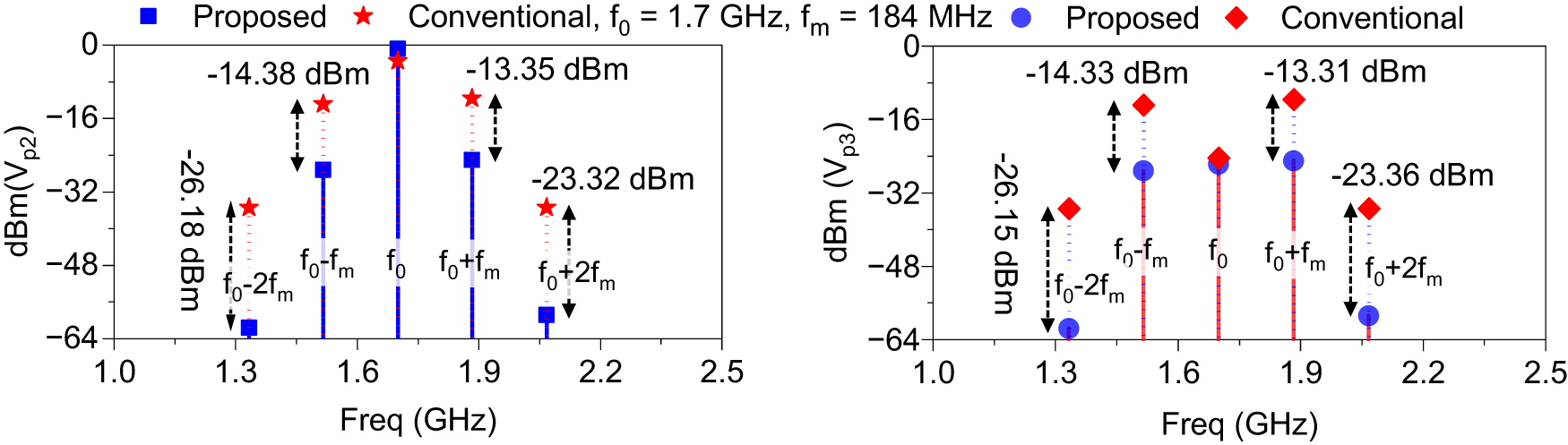
Figure 11 shows the output spectra when a signal of 0 dBm power at RF carrier frequency (f 0) of 1.70 GHz is excited at input port 1. As observed from the results, a 14.38 dB reduction in IM signal power at f 0-fm = 1.516 GHz and a 13.35 dB reduction at f 0 + fm = 1.884 GHz can be observed as compared to a conventional circulator. The power reduction at these IM product terms leads to a 1.39 dB improvement in transmission IL as compared to a conventional circulator.
Simulated output spectra at transmission output port 2 and isolation port 3 when 0 dBm of input power at the input port 1 with RF carrier frequency (f 0) of 1.70 GHz is excited. Circuit parameter values: g 0 = 1, g 1 = g 3 = 0.9146, g 2 = 0.6857, A 0 = 1, BWstatic = 90 MHz, and  $Q_u^s\,$=
 $\,Q_u^m$ = 500. Modulation parameters: fm = 184 MHz, m = 0.182.

Experimental results
For proof-of-concept, the proposed circulator is designed and fabricated using a microstrip line on a Taconic substrate with a dielectric constant of 2.2 and a thickness of 0.787 mm. The design goals are to achieve low transmission IL and high reverse IX across a tunable frequency range from 1.40 to 1.80 GHz.
Figure 12(a) and 12(b) shows the microstrip line implementations of the static and time-modulated resonators. The static resonators are realized using TLs with lengths L 1, L 2 and widths W 1, W 2, and varactor diode 1T362 from Sony Inc [29]. The desired resonant frequencies of the static resonators can be achieved by appropriately selecting values of W 1, W 2, L 1, L 2, and varactor diode capacitances. Similarly, the time-modulated resonators are implemented using TLs (W 2/L 2), dc-block capacitor (C dc), and varactor diode SMV 1233-079LF from Skyworks Inc [30]. In practice, the time-varying capacitors (C 2(t)) in each branch of the time-modulated resonators are realized by modulating varactor diodes with sinusoidal signals applied TLs (W b/L b).
Microstrip line implementation of the proposed circulator using mixed static and time-modulated resonators: (a) static resonator, (b) time-modulated resonator, (c) coupling between port and static resonator, (d) coupling between static and time-modulated resonators, and (e) overall microstrip line implementation.

The desired coupling between the ports and static resonators (i.e. K 01) is realized by appropriately optimizing the values of W 1, L c1, and g 1, as shown in Figure 12(c). Similarly, the desired coupling between the static and time-modulated resonators (i.e. K 12) is achieved by controlling the values of L 2, W 2, and g 2, as illustrated in Figure 12(d). Figure 12(e) presents the overall microstrip line implementation of the circulator. The physical dimensions of the proposed microstrip line circulator are optimized through co-simulations using Keysight ADS and ANSYS HFSS 2024, in combination with SPICE models of varactors [Reference Xu and Piazza24, Reference Kord, Sounas and Alu25], as well as lumped capacitors. The optimized physical dimensions of the circulator are also shown in Figure 12(e).
Figure 13 shows the photograph of the fabricated circulator along with the experimental setup. The sinusoidal modulation signals with progressive phase shifts are applied through Keysight signal generators, while the S-parameters are measured using Keysight PNA 5224B vector network analyzer.
Photograph of a fabricated circuit with S-parameters measurement setup.

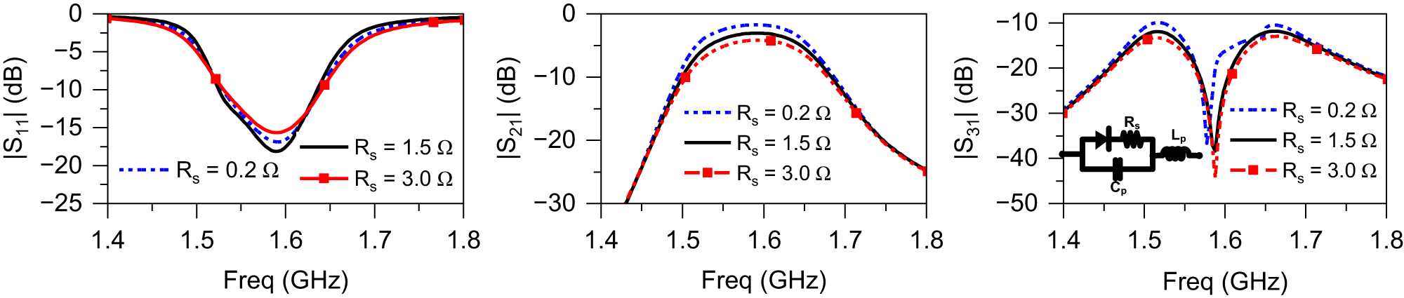
Figure 14 shows the simulated and measured S-parameters of the fabricated circulator, and measured results are summarized in Table 1. The measured results align closely with simulation results. In the measurement, the frequency is continuously tuned from 1.45 to 1.70 GHz (i.e. tuning ratio of 1:1.1724) by varying the bias voltage of varactor diodes and modulation parameters. The measured transmission IL is varied from 3.95 to 4.60 dB while IX is varied from 40.5 to 19.05 dB at f 0. Additionally, the input and output return losses exceed 15 dB for all tuning states. The transmission IL has mainly occurred due to the parasitic resistance of varactor diodes. In the measurement, only one null is observed in reverse IX because two nulls are very near and merged into one due to the low quality factor of varactor diodes.
Simulated and measured frequency responses of the fabricated circulator using mixed static and time-modulated resonators. Modulation parameters: fm = 180 MHz, Vm = 2.4 V.

Measurement results summary

To investigate the cause of the forward transmission IL, we performed a simulation of the microstrip line circulator using the SPICE model of varactor diodes SMV1233 and 1T362 [29, 30], and the results are shown in Figure 15. The simulation indicates that forward transmission IL increases as the parasitic resistance Rs of varactor diode increases. The forward transmission IL can be improved by employing varactor diodes with smaller parasitic resistance.
Simulated frequency responses with different parasitic resistance values of the varactor diodes.

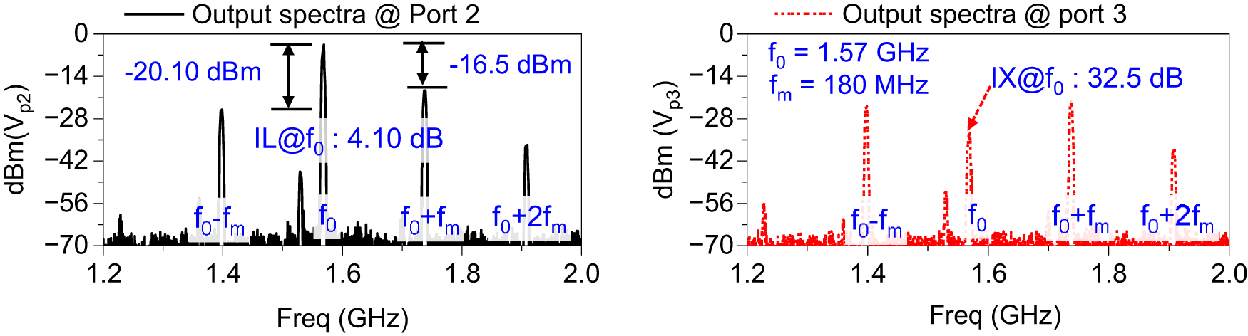
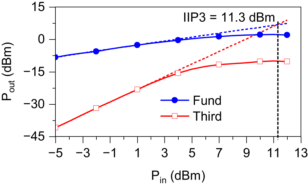
Figure 16 depicts the measured output spectra at ports 2 and 3 when a signal of 0-dBm input power at RF (f 0) of 1.58 GHz is excited at input port 1. These results indicate output spectra of −24.5 dBm at f 0 − fm = 1.40 GHz while −21.10 dBm at f 0 + fm = 1.76 GHz. Figure 17 shows the measured third-order input intercept point (IIP3) using two signals separated by 2 MHz at a center frequency of 1.58 GHz (i.e. f 1 = 1.579 and f 2 = 1.581 GHz). The output power (Pout) at fundamental frequencies (i.e. f 1 and f 2) and third-order IM product (i.e. 2f 1 − f 2 and 2f 2 − f 1) are measured and extrapolated to determine the IIP3. The measured IIP3 is 11.3 dBm.
Measured output spectra at ports 2 and 3 when input power of 0 dBm at RF center frequency of f 0 = 1.575 GHz is excited at port 1. Modulation parameters: fm = 180 MHz, V m = 2.40 V, V dc1 = 2.20 V, and V dc2 = 20 V.

Measured third-order input intercept point (IIP3) with two-tone input signals separated by 2 MHz at the center frequency (f 0) of 1.575 GHz. Modulation parameters: fm = 180 MHz, V m = 2.40 V, V dc1 = 2.2 V, and V dc2 = 20 V.

Table 2 presents a performance comparison with state-of-the-art. As summarized in the table, ferrite-based circulators provide relatively lower IL; however, they are bulky, expensive, and incompatible with IC technologies. Previously reported STM-based circulators [Reference Estep, Sounas and Alu17, Reference Kord, Sounas, Xiao and Alu19, Reference Kadry, Alhawari and Sounas21], exhibit relatively high IL, limited IM signal power reduction [Reference Kord, Sounas and Alu25], and lack tunable frequency characteristics. In paper [Reference Wu and Liu26], an STM-based circulator employs hybrid static and time-modulated resonators; however, its operating frequency remains fixed and cannot be tuned. In contrast, the proposed circulator offers frequency-tunable characteristics and suppressed IM signal power.
Performance comparison with state-of-the-art

Mixed type: static and time-modulated resonators, f 0: RF center frequency, fm: modulation frequency, first-order IM: f 0 ± fm.
Conclusion
This paper demonstrated a comprehensive analysis and design methodology of spatiotemporal modulated frequency-tunable circulator utilizing a combination of static and time-modulated resonators. Analytical design equations are derived to enable comprehensive analysis and provide clear insight into the nonreciprocity mechanism of the time-modulated circulator. To investigate the cause of insertion loss in practical design, the unloaded quality factors of both static and time-modulated resonators are incorporated into the spectral admittance matrices. Numerical results show that coupling of high quality-factor static and time-modulated resonators at each branch enables the achievement of low in-band transmission loss, high isolation, and good port matching characteristics. Furthermore, the coupling of the static resonator and time-modulated resonators suppresses IM product signal power, thereby improving transmission insertion loss. To validate this concept, a magnetless microstrip line circulator with tunable frequency response is designed and fabricated. The measured results are well agreed with simulations.
Funding statement
This research was supported by the Basic Science Research Program through the NRF grant funded by the Ministry of Education (RS-2019-NR040079, 50%) and in part by the Institute of Information and Communications Technology Planning and Evaluation (IITP) Innovative Human Resource Development for Local Intellectualization program grant funded by the Korean government (MSIT) (IITP-2026-RS-2024-00439292, 50%).
Competing interests
The authors declare none.

Girdhari Chaudhary received the B.E. (2004) and M. Tech. (2007) in Electronics and Communication Engineering from Nepal Engineering College (NEC), Kathmandu, Nepal, and MNIT, Jaipur, India, as well as PhD in Electronics Engineering (2013) from Jeonbuk National University, Republic of Korea. He is currently working as Research Associate Professor at Jeonbuk RICE Intelligence Innovation Research Center, Jeonbuk National University, South Korea. From March 2021 to August 2024, he worked as a contract professor at JIANT-IT Human Resource Development Center, Jeonbuk National University, Korea. Previously, he also worked as Principal Investigator (PI) of an independent Project through the Basic Science Research Program of the National Research Foundation (NRF), funded by the Ministry of Education, Korea. He is also a recipient of the BK21 PLUS Research Excellence Award 2015 and Korean Research Fellowship (KRF) through the NRF of Korea funded by the Ministry of Science and ICT. His research interests include multi-band tunable passive circuits, in-band full-duplex systems and high-efficiency power amplifiers, negative group delay circuits and their applications. Dr Chaudhary is a senior member of IEEE and a member of the European Microwave Association (EuMA) and has served as a reviewer of IEEE Transactions on Microwave Theory and Techniques, IEEE Microwave and Wireless Components Letters, IEEE Transactions on Circuits and Systems-I, and IEEE Transactions on Industrial Electronics.

Palaystint Thorng rececation and Electronics Engineering from the Royal University of Phnom Penh, Cambodia, in 2022. He is currently pursuing the integrated M.E. and PhD degree in electronic engineering at Jeonbuk National University, South Korea,. His research focuses on advanced digital predistortion techniques for wideband power amplifiers in next-generation wireless systems, AI-based behavioral modeling of RF power amplifiers, and machine learning, particularly neural network architectures, for power amplifier linearization and performance enhancement.

Suyeon Kim received the bachelor’s degree in Electronics Engineering from Jeonbuk National University, Republic of Korea, in 2025. She is currently pursuing the M.E. degree in Electronics and Information Engineering at Jeonbuk National University, Republic of Korea. Her research interests include microwave power divider/combiner design, high-efficiency RF power amplifiers, and microwave circuit design.

Yongchae Jeong received the BSEE, MSEE, and Ph.D. degrees in Electronic Engineering from Sogang University, Seoul, Republic of Korea in 1989, 1991, and 1996, respectively. From 1991 to 1998, he worked as a senior engineer with Samsung Electronics, Korea. In 1998, he joined the Division of Electronic Engineering, Jeonbuk National University, Jeonju, Republic of Korea. From July 2006 to December 2007, he joined the Georgia Institute of Technology as a visiting professor. Since July 2024, Prof. Jeong has been serving as the Director of Jeonbuk RICE Intelligence Innovation Research Center, Jeonbuk National University. He also served as the Vice-President of Plan Affairs and the Director of HOPE-IT Human Resource Development Center of BK21 PLUS, Jeonbuk National University. He teaches and conducts research in microwave passive and active circuits, mobile and satellite base-station RF systems, design of periodic defected transmission lines, negative group delay circuits and their applications, in-band full-duplex radio and RFIC design. Prof. Jeong is a senior member of IEEE and a member of KIEES (Korea Institute of Electromagnetic Engineering and Science). He has authored and co-authored over 320 papers in international journals and conference proceedings.









 Open access

