Implications
Robustness of animals and uniformity of end product can be improved by exploiting genetic variation in uniformity in breeding programs. The aim of this study was to estimate genetic variation in uniformity of body weight of broilers. Data from a commercial dam line were used and analyzed with different models. Although heritability of uniformity was low (0.03 to 0.05), a relatively high genetic variation was estimated as indicated by high genetic coefficients of variation (0.35 to 0.57). Surprisingly, uniformity in females and males was not correlated. Nevertheless, results indicate that uniformity can be improved by means of genetic selection.
Introduction
Uniformity of body weight of broilers is of economic interest, because slaughterhouses want to produce homogeneous products. As a consequence, producers get price penalties when too many broilers delivered to the slaughterhouse are outside the preferred range. Management and breeding strategies can be used to improve uniformity (Hohenboken, Reference Hohenboken1985), but selective breeding for uniformity in livestock breeding programs can be useful only if it varies genetically.
There is some empirical evidence that genetic variation in residual variance exists. SanCristobal-Gaudy et al. (Reference SanCristobal-Gaudy, Bodin, Elsen and Chevalet2001), Sorensen and Waagepetersen (Reference Sorensen and Waagepetersen2003), Ros et al. (Reference Ros, Sorensen, Waagepetersen, Dupont-Nivet, SanCristobal, Bonnett and Mallard2004), Gutierrez et al. (Reference Gutierrez, Nieto, Piqueras, Ibanez and Salgado2006) and Ibanez-Escriche et al. (Reference Ibanez-Escriche, Moreno, Nieto, Piqueras, Salgado and Gutierrez2008a and Reference Ibanez-Escriche, Varona, Sorensen and Noguera2008b) used a structural model for heterogeneous residual variance and found substantial genetic variation in residual variance for litter size in sheep, litter size in pigs, body weight in snails, litter size and weight in mice, body weight traits in mice, and slaughter weight in pigs, respectively. Rowe et al. (Reference Rowe, White, Avendano and Hill2006) found substantial genetic heterogeneity of residual variance between sire families in body weight of broilers. Probably the clearest example is by Mackay and Lyman (Reference Mackay and Lyman2005), who derived 300 isofemale lines of Drosophila melanogaster and found substantial highly significant genetic variance in residual variance between lines under controlled laboratory conditions.
If there is genetic variance in residual variance, it should be possible to change it by selection. Phenotypic variance changed in some selection experiments with Drosophila melanogaster or Tribolium, with stabilizing selection or divergent selection on phenotypic variance (Rendel et al., Reference Rendel, Sheldon and Finlay1966; Kaufman et al., Reference Kaufman, Enfield and Comstock1977; Cardin and Minvielle, Reference Cardin and Minvielle1986), while it did not in an experiment with mice (Falconer and Robertson, Reference Falconer and Robertson1956). More recently, Larzul et al. (Reference Larzul, Le Roy, Tribout, Gogue and SanCristobal2006) did not find conclusive results in selection of pigs on high or low residual variability of muscle pH, but Garreau et al. (Reference Garreau, Bolet, Larzul, Robert-Granie, Saleil, SanCristobal and Bodin2008) found significant responses in residual variance in rabbits when selecting on high or low residual variance of birth weight. The relatively substantial responses obtained by Garreau et al. (Reference Garreau, Bolet, Larzul, Robert-Granie, Saleil, SanCristobal and Bodin2008) seem to support the large responses in residual variance predicted by Mulder et al. (Reference Mulder, Bijma and Hill2007 and Reference Mulder, Bijma and Hill2008) using simulation, whereas the study of Larzul et al. (Reference Larzul, Le Roy, Tribout, Gogue and SanCristobal2006) lacked power because of small numbers of sires and small numbers of progeny per sire.
One of the main problems with analysis of genetic heterogeneity of residual variance is its estimability. Rowe et al. (Reference Rowe, White, Avendano and Hill2006) used a two-step approach, in which the first stage used a model to analyze body weight with allowance for differences in residual variance among sire families, and in the second stage the variation among these estimates of the residual variance were analyzed with least squares. In some studies, log transformed squared residuals have been analyzed, also using a two-step approach (Larzul et al., Reference Larzul, Le Roy, Tribout, Gogue and SanCristobal2006; Bolet et al., Reference Bolet, Garreau, Joly, Theau-Clement, Falieres, Hurtaud and Bodin2007), which gives the flexibility to account for environmental effects on the residual variance at the level of the record that is not possible in the least squares analysis of Rowe et al. (Reference Rowe, White, Avendano and Hill2006). Ideally, one would simultaneously fit a model for the mean of the trait (e.g. body weight) and for the residual variance using a structural model. Sorensen and Waagepetersen (Reference Sorensen and Waagepetersen2003), Ros et al. (Reference Ros, Sorensen, Waagepetersen, Dupont-Nivet, SanCristobal, Bonnett and Mallard2004) and Gutierrez et al. (Reference Gutierrez, Nieto, Piqueras, Ibanez and Salgado2006) applied these structural models in a Bayesian context, implemented using Markov chain Monte Carlo sampling (MCMC). The disadvantages of those methods are that there is no standard software package available and no extension has yet been made to estimate genetic correlations between residual variances of different traits or of different sexes. Therefore, in this study, we have applied the two-step approach of Larzul et al. (Reference Larzul, Le Roy, Tribout, Gogue and SanCristobal2006) and Bolet et al. (Reference Bolet, Garreau, Joly, Theau-Clement, Falieres, Hurtaud and Bodin2007), and extended this to bivariate analyses using standard REML-software.
The objectives of this study were to estimate genetic variance in residual variance for body weight in broilers, and to estimate the genetic correlations between the additive genetic effects for the mean and the residual variance and between female and male residual variance. It therefore provides a confirmation of the results of Rowe et al. (Reference Rowe, White, Avendano and Hill2006) and those recently presented by Wolc et al. (Reference Wolc, White, Avendano and Hill2009) using a different population of broilers and different analytical approaches.
Material and methods
Data
The data were provided by Hendrix Genetics, Boxmeer, the Netherlands, and comprised 106 818 records of body weight of birds of a maternal dam line with ongoing selection on number of eggs, breast meat, feed conversion, and average daily gain. Birds were weighed at an age between 37 and 60 days. Data were collected between 1 January 1995 and 1 June 2007. Birds were wing banded at day of hatching. Birds of both sexes were housed in two housing systems – floor housing and cage housing – and were fed ad libitum. From each sire family some birds were housed in cages at 3 weeks of age to measure feed conversion. The barns were fully controlled with temperature and light schemes as used in standard commercial broiler husbandry. The pedigree file comprised 123 328 animals and traced back at least four generations, so that younger animals had longer pedigrees.
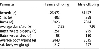
First a few general edits were applied. Records of body weights over 3.5 phenotypic standard deviations from the mean were excluded (73 records < mean − 3.5 s.d.; 143 records > mean + 3.5 s.d.), considered a suitable compromise between removing severe abnormalities and minimizing the effect of data trimming on the estimated genetic variance in residual variance. Owing to very few records in some age classes, records on birds weighed outside the range 43 to 53 days were excluded (595 records), to minimize the age range. From this data set (106 007 records) two edited data sets were extracted: one for females, the other for males. For each data set, sire families were selected which had at least 50 offspring of one sex, and classes for the interaction between hatch week of the individual and the hatch week of its dam (hwihwd) were selected if they had at least five animals. These requirements were met by 402 sire families and 26 972 records of females, and 369 sires and 24 407 records of males. The requirements of 50 offspring per sire and five animals per hwihwd halved the size of the data sets. Table 1 shows some characteristics of these two data sets.
Summary statistics of the female and male data set

Analysis
The female and male data were analyzed separately to quantify genetic variation in residual variance using the two-stage method (Larzul et al., Reference Larzul, Le Roy, Tribout, Gogue and SanCristobal2006; Bolet et al., Reference Bolet, Garreau, Joly, Theau-Clement, Falieres, Hurtaud and Bodin2007).
First stage: estimation of genetic variance in body weight
In all analyses, body weight data for each sex separately were first analyzed with an animal model using ASREML (Gilmour et al., Reference Gilmour, Gogel, Cullis and Thompson2006), accounting for differences between sire families in residual variance:

where yijkln is body weight of individual i, which has sire o and dam n, μ is the overall mean, hj is the housing system effect j (floor and cage system), agek is the effect for age class k (9 classes), hwihwdl is the joint effect l of the hatch week of the individual and the hatch week of its dam (1515 classes for females and 1521 for males),  is the random genetic animal effect for the mean for individual i (variance
 ), Dn is the random maternal environmental effect of dam n (variance
 ) and
 is the residual error with variance
 for sire family o. The hwihwd-effects accounted for time effects when the dam was hatched and when the bird itself was hatched, such as seasonal effects. A model including maternal genetic effects was also tested, but did not converge for the male data set and only slightly improved likelihood for females. Therefore, maternal genetic effects were not considered in this study. In contrast to the sire and dam model used by Rowe et al. (Reference Rowe, White, Avendano and Hill2006) and Wolc et al. (Reference Wolc, White, Avendano and Hill2009), an animal model was chosen so that the residual variance was expected to be less confounded with Mendelian sampling variance and had substantially higher likelihood than a sire–dam model (females: +17; males: +29); although a formal likelihood ratio test (LR-test) can not be applied here because these models are not nested. For model comparison, the model in equation
was also fitted assuming a homogeneous residual variance structure.
Second stage: estimation of genetic variance in residual variance
The residuals from equation (1) were transformed by using the natural log of the squared residuals ( ) to reduce the dependency of
 on its variance and non-normality of the distribution of
 . Density plots showed that the log-transformation did not completely remove non-normality, but simulation showed that the transformation was adequate to estimate genetic variance.
The log-transformed squared residuals,  , were analyzed as a trait. The same fixed effects were fitted as for body weight, but in this case the fixed effects (denoted * to distinguish them from those in the first stage) account for differences in
 between different fixed effect levels due to environmental heterogeneity of residual variance. The model is:

where  is the additive genetic value of animal i for
 (variance
 ) and
 is the residual effect. In equation
, a constant residual variance (variance  ) was assumed for
 . The maternal environmental effect was excluded from the model because its variance was not significantly different from zero.
Estimation of a genetic correlation between the mean and the residual variance
To estimate the genetic correlation between the additive genetic effects for the mean and the residual variance, bivariate analyses were carried out iteratively, updating  for each of 20 iterations. Each iteration comprised an ASREML-run, which was considered converged when the REML-likelihood changed less than 0.002 × iteration number (<20), and the individual variance parameter estimates changed less than 1% between successive iterations (Gilmour et al., Reference Gilmour, Gogel, Cullis and Thompson2006). The bivariate analysis can be written in matrix notation as:
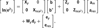
where y is the vector of yijkln; ln(e2) is the vector of  ; Xy and
 are the incidence matrices for the fixed effects for body weight and
 , respectively; b and b* are the solution vectors for the fixed effects;
 and
 are the incidence matrices for the additive genetic effects
 and
 ; am and ares are the solution vectors with estimates of
 and
 ; Wy is the incidence matrix for maternal environmental effects that are modeled only for body weight; dy is the solution vector for the random maternal environmental effect Dn; and ey and eres are the vectors with residuals for body weight (=
 in equation (1)) and
 (=
 in equation (2)). The vector ln(e2) was updated in each iteration using ey of the previous iteration. The additive genetic effects Am and Ares are assumed bivariate normally distributed as

 , A is the additive genetic relationship matrix,
 and
 is the genetic correlation between Am and Ares. The residuals ey and eres are assumed bivariate normally distributed as
 , where I is the identity matrix and
 including heterogeneous residual variances per sire family o for body weight and homogeneous residual variance for eres. The residuals
 and
 are assumed uncorrelated, because cov(e,e 2) = 0 when e is normally distributed. Parameter estimates oscillated somewhat (the standard deviation of parameter estimates was less than 5% of the average parameter estimate) between two very similar sets of parameters after the first five to ten iterations; therefore, results are presented as the average of the last ten iterations. Oscillations can be explained by the interplay between
 , the residual
 and the other effects in the model. When
 increases, the residual
 decreases and therefore
 decreases; and when
 and
 are genetically correlated, one will also affect the other directly. Both mechanisms explain the oscillations.
Estimation of a genetic correlation between female and male residual variance
To calculate the genetic correlation between the additive genetic effects for the residual variance in females and males, the data sets were combined using  of iteration 20 of equation (3). The bivariate analysis in matrix notation can be written as:
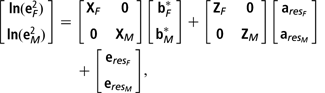
where the effects are the same as in equation (3), but now with subscripts F and M to indicate whether it is for females and males,  and
 are assumed to be bivariate normally distributed as
 , where
 , where
 is the genetic correlation between
 and
 . The residuals
 and
 are assumed to be bivariate normally distributed as
 , where
 .
Calculation of quantitative genetic parameters
To facilitate interpretation and implications for breeding, two standardized parameters were calculated: the heritability of residual variance  and the genetic coefficient of variation GCVE. Both
 and GCVE are possible measures to choose: the former largely determines the accuracy of estimated breeding value (EBV) for residual variance and the latter, the size of the possible selection response relative to the current residual variance. These were calculated as
 and
 , where
 and
 is the average residual variance (Mulder et al., Reference Mulder, Bijma and Hill2007). Therefore, the genetic variance in
 needs to be converted to
 , which is the genetic variance of the additive genetic effect for residual variance (Av) in the quantitative genetic model for genetic heterogeneity of residual variance (Hill and Zhang, Reference Hill and Zhang2004; Mulder et al., Reference Mulder, Bijma and Hill2007). The genetic variance
 can be calculated as
 , where
 is the heritability of
 .
The heritability of the mean was calculated as 
 and the maternal environment variance ratio as
 . Approximate standard errors were calculated for estimated variance components and variance ratios using ASREML (Gilmour et al., Reference Gilmour, Gogel, Cullis and Thompson2006). For
 , the standard error was crudely approximated as
 . For GCVE and
 , no simple approximations were available to calculate the standard error.
Comparison of models with and without heterogeneity of sire-family residual variance
The model variants in equation (1), with and without heterogeneity of residual variance, were compared using a LR-test, assuming χ 2 with ns − 1 degrees of freedom for the increase from fitting estimated variance components (one for each of ns sires) in the full model compared to the reduced model of homogeneity (Wilks, Reference Wilks1938). REML likelihoods were obtained from ASREML. Models were also compared using Akaike’s information content (AIC) (Akaike, Reference Akaike1973) and the Bayesian or Schwarz information criterion (BIC) (Schwarz, Reference Schwarz1978) to penalize those with a large number of parameters. BIC produces a more drastic penalty than AIC, which increases with sample size.
Relationships between sire EBV and residual variance of offspring
Plots were used to visualize the relationship between sire EBV for residual variance (equation (3)) and the observed log-transformed residual variance of its offspring (i.e. the phenotypic variance corrected for fixed effects, genetic effects for the mean and maternal environmental effects), which would be of relevance when improving uniformity by selection. EBVs ( ) of iteration 20 of the bivariate analyses (equation (3)) were used. To quantify the strength of the relationship, correlations were calculated between these EBVs and the observed log-transformed residual variance of its offspring.
Results
Comparison of models with homogeneous or heterogeneous residual variance among sire families
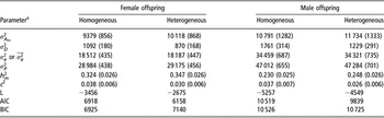
Table 2 shows estimated variance components, estimates of variance ratios and likelihood-based parameters for females and males for models (equation (1)) with homogeneous and heterogeneous residual variances among sire families. For both sexes, fitting heterogeneous residual variance for each sire family increased the estimates of genetic variance in mean body weight ( ) and decreased those for maternal environmental variance (
 ). Estimated variance components, especially the average residual variance
 , were larger for males than for females, resulting in a larger
 (
 ) for females. A model with heterogeneous residual variances among sire families fitted significantly better than one with a homogeneous residual variance (LR-test: P < 0.001). Taking into account the number of parameters estimated, it is not obvious which model is better because the AIC is lower (i.e. better fit), but the BIC is higher (i.e. poorer fit) for the model with heterogeneous residual variance among sire families.
Variance component estimates, estimates of variance ratios and likelihood-based parameters for body weight (g) of females and males using models (equation (1)) with homogeneous or heterogeneous residual variance structure (approximate s.e. within brackets)

a is the estimated genetic variance in the additive genetic effect for the mean Am;
 is the estimated variance of the maternal environmental effect;
 or
 is the (average) estimated residual variance with homogeneous (heterogeneous) residual variance per sire family; σ 2P is the estimated phenotypic variance
 ;
 ;
 , L is log-likelihood; AIC is Akaike’s information criterion and BIC is the Bayesian information criterion.
Genetic variation in residual variance
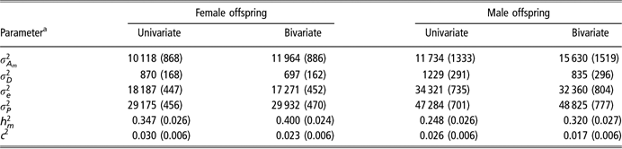
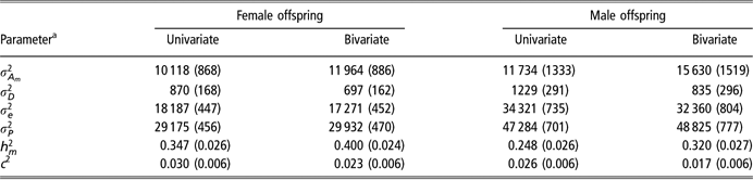
Table 3 shows estimates of genetic variance in residual variance using a univariate (equation (2)) and a bivariate analysis (equation (3)) to analyze data for females and males. Estimates of  deviated significantly from zero (P < 0.001). With the bivariate analysis estimates of
 ,
 and GCVE increased substantially in comparison to the univariate analysis. Table 4 shows that
 and
 also increased, while the maternal environment variance and c 2 decreased with the bivariate analysis. It can be concluded that substantial genetic variance in residual variance exists for body weight of broilers. Accounting for genetic heterogeneity of residual variance also affects conventional genetic parameters, such as the usual heritability of the mean
 .
Comparison of estimated genetic variance in residual variance of body weight (g) (approximate s.e. within brackets for  and
 ) using univariate or bivariate analysisFootnote a for male and female broilers

a In the univariate analysis only log-transformed squared residuals (equation (2)) are analyzed; in the bivariate analysis body weight and its log-transformed squared residuals (equation (3)) are analyzed with iterative updating of the residuals.
b  is the estimated genetic variance of the additive genetic effect Ares for ln(e 2) (equation (2));
 is the estimated genetic variance for Av in the quantitative genetic model for genetic heterogeneity of residual variance (Hill and Zhang, 2004; Mulder et al., 2007);
 and

Genetic correlation between mean and residual variance and between female and male residual variance
The estimates from the bivariate analysis of body weight and log-transformed squared residuals (equation (3)) of the genetic correlations between Am and Ares ( ) were −0.41 (s.e. = 0.032) and −0.45 (s.e. = 0.040) in females and males, respectively. The estimate of
 , the genetic correlation between female and male residual variance (equation (4)), was very small: 0.11 (s.e. = 0.089).
Relationships between sire EBV for residual variance and the observed residual variance of offspring
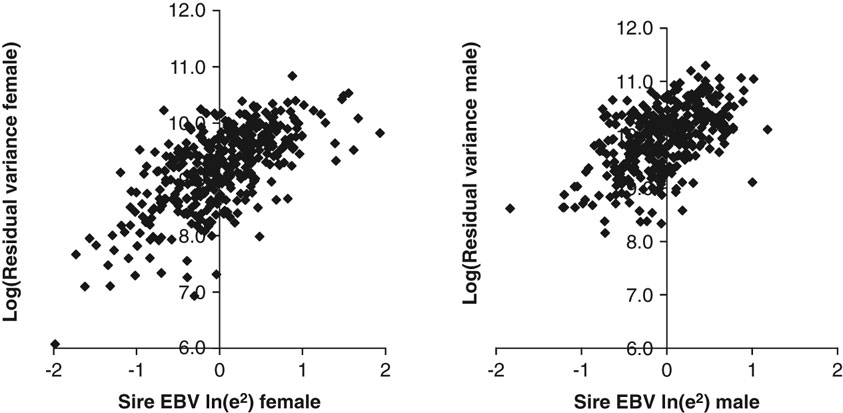
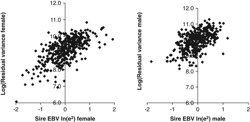
The scatter plots of log-transformed residual variance of female and male offspring as a function of  and
 in Figure 1 show that there was substantial variability in residual variance between sires. There was a positive trend between the EBVs for residual variance and the observed log-transformed residual variance, but there was also substantial noise, especially for male offspring. The correlation between
 and log-transformed residual variance of female offspring was 0.65, and the equivalent for male offspring was 0.54.
Scatter plots of residual variance of female and male offspring as a function of the sire’s estimated breeding value (EBV) based on log-transformed squared residuals (ln(e 2)) ( and
 ).
Discussion
In this study, it was shown that there is substantial genetic variation in residual variation, the so-called genetic heterogeneity of residual variance, for body weight in broilers. A REML-analysis on log-transformed squared residuals was used (e.g. Larzul et al., Reference Larzul, Le Roy, Tribout, Gogue and SanCristobal2006; Bolet et al., Reference Bolet, Garreau, Joly, Theau-Clement, Falieres, Hurtaud and Bodin2007) and extended to multivariate approaches to estimate genetic correlations between the additive genetic effects for mean and residual variance, and between additive genetic effects for residual variance in males and females. The iterative bivariate analysis with body weight itself and log-transformed squared residuals of body weight was closest to a structural model, as suggested by SanCristobal-Gaudy et al. (Reference SanCristobal-Gaudy, Elsen, Bodin and Chevalet1998) and Sorensen and Waagepetersen (Reference Sorensen and Waagepetersen2003). It had a side effect in that the estimate of  increased by 15% in females and 29% in males, thereby increasing the accuracy of
 , unless the genetic variance in mean (
 ) is biased upwards and the residual variance (σ 2e) is biased downward. A similar trend was also observed by Sorensen and Waagepetersen (Reference Sorensen and Waagepetersen2003), who observed an increase of 15% in
 when extending a model with homogeneous residual variance to a model with genetically structured residual variances. Ibanez-Escriche et al. (Reference Ibanez-Escriche, Moreno, Nieto, Piqueras, Salgado and Gutierrez2008a) reported increases in additive genetic variance of the mean between 28% and 200%.
The method used, incorporates both genetic and environmental effects on the residual variance, but heterogeneous residual variance and effects on the mean are not estimated simultaneously at the level of individual records. Although in principle less appealing, the current method is flexible and can be applied in standard REML-software. This enables the study of genetic relationships between residual variances of different traits, environments, and so on, and can be applied to breeding value estimation using standard BLUP-software (e.g. Lidauer and Stranden, Reference Lidauer and Stranden1999), in contrast to a structural model in a Bayesian context implemented using MCMC sampling. The same two-step method was used in selection experiments to change the residual variance (Larzul et al., Reference Larzul, Le Roy, Tribout, Gogue and SanCristobal2006; Bolet et al., Reference Bolet, Garreau, Joly, Theau-Clement, Falieres, Hurtaud and Bodin2007; Garreau et al., Reference Garreau, Bolet, Larzul, Robert-Granie, Saleil, SanCristobal and Bodin2008). The method presented here was tested using simulations with one generation of parents and offspring, and results showed that it is able to estimate genetic variance in residual variance. Wolc et al. (Reference Wolc, White, Avendano and Hill2009) used a similar REML approach as in this study and also a Bayesian approach, and the two methods yielded similar results. In this study, the BIC favored the model with homogeneous residual variance, although both the LR-test and AIC favored the model with heterogeneous residual variance per sire family. This probably indicates that the residual variances were estimated with low accuracy in each sire family rather than the absence of heterogeneity of residual variance. Future research may focus on evaluating different modeling approaches.
In general, estimates of  obtained here are higher than those of Rowe et al. (Reference Rowe, White, Avendano and Hill2006), who used a different method and data set. When the least-squares method of Rowe et al. (Reference Rowe, White, Avendano and Hill2006) was applied to the current data set, however, estimates of
 were higher: 0.088 in females and 0.087 in males. The large difference found using the same method is probably due to more severe confounding of genetic and environmental heterogeneity of residual variance, because the data in this study spanned a longer time period than for Rowe et al. (Reference Rowe, White, Avendano and Hill2006) and because the ages at which birds were weighed ranged more widely, between 43 and 53 days of age, possibly introducing an extra source of heterogeneity. Wolc et al. (Reference Wolc, White, Avendano and Hill2009) used data that partly overlapped those in the study of Rowe et al. (Reference Rowe, White, Avendano and Hill2006) and estimates of
 were very similar to those of our univariate analysis. Estimates of
 from studies in other species (e.g. SanCristobal-Gaudy et al., Reference SanCristobal-Gaudy, Bodin, Elsen and Chevalet2001; Sorensen and Waagepetersen, Reference Sorensen and Waagepetersen2003; Ros et al., Reference Ros, Sorensen, Waagepetersen, Dupont-Nivet, SanCristobal, Bonnett and Mallard2004) are in the same range as those obtained here (see review in Mulder et al. (Reference Mulder, Bijma and Hill2007)). The estimate of the genetic correlation between the additive effects for the mean and the residual variance (
 ) was more negative in this study than obtained by Rowe et al. (Reference Rowe, White, Avendano and Hill2006). Variation in estimates of this genetic correlation between studies is large, although generally negative for body weight traits. Estimates obtained were −0.07 for slaughter weight in pigs (Ibanez-Escriche et al., Reference Ibanez-Escriche, Varona, Sorensen and Noguera2008b), −0.31 and −0.38 for body weight at two ages in mice (Ibanez-Escriche et al., Reference Ibanez-Escriche, Moreno, Nieto, Piqueras, Salgado and Gutierrez2008a) but, exceptionally, a highly positive genetic correlation of 0.81 for adult body weight in snails (Ros et al., Reference Ros, Sorensen, Waagepetersen, Dupont-Nivet, SanCristobal, Bonnett and Mallard2004).
In this study, body weights of females and males were analyzed separately because they differ greatly in the variance of observations. A large difference in estimated variance components and estimated variance ratios (Tables 3 and 4) was found between them; rather more extreme than in the studies of Rowe et al. (Reference Rowe, White, Avendano and Hill2006) and Wolc et al. (Reference Wolc, White, Avendano and Hill2009). The large difference in  indicates that it might be advantageous in breeding value estimation to use different variance ratios for female and male offspring. The genetic correlation between female and male residual variance was close to zero, rather surprisingly indicating that these traits have different genetic bases. Whilst Rowe et al. (Reference Rowe, White, Avendano and Hill2006) also found a low correlation for ln(s 2) between sexes, Wolc et al. (Reference Wolc, White, Avendano and Hill2009) obtained an estimate of the genetic correlation of 0.36 using an improved method. It would be useful to understand the basis of these low correlations; but, assuming they are real, it is recommended that the body weight and (log-transformed) squared residuals of females and males be analyzed as four different traits.
Genetic heterogeneity of residual variance may have biological meaning in terms of environmental sensitivity, disease resistance, biological limits and mean–variance relationships. Genotypes that are very sensitive to changes in micro-environment (e.g. feed changes, weather changes and so on) would have a larger residual variance than those insensitive to such changes. The moderate negative genetic correlation between the additive genetic effects for the mean and the residual variance may indicate that animals with a higher mean are also less sensitive; but another explanation is that animals with a lower mean are more sensitive to diseases and have higher residual variance because of higher disease incidence. Therefore, mixture models for diseased and non-diseased animals (e.g. Odegard et al., Reference Odegard, Madsen, Gianola, Klemetsdal, Jensen, Heringstad and Korsgaard2005) and models for genetic heterogeneity of residual variance might capture part of the same genetic information. If there is a biological limit caused by an environmental constraint (e.g. restricted feeding) it may also create a negative genetic correlation between the mean and the residual variance, because the variability would be reduced on one side of the distribution. A positive mean–variance relationship (scale effect), however, would create a positive genetic correlation between the mean and the residual variance, in contrast to the negative genetic correlation found here.
This study shows that there is substantial genetic variation in residual variance (high genetic coefficient of variation, GCVE). Although the underlying model is slightly different, we use the methodology of Mulder et al. (Reference Mulder, Bijma and Hill2008) to show what could be achieved in a breeding program based on sib-testing with 50 half-sibs. Based on the estimates obtained,  between 2.9% and 4.7% and GCVE between 0.35 and 0.57, it would be possible to decrease the residual variance by 20% to 30% when selecting solely on it for one generation. The phenotypic standard deviation would then be substantially reduced, for example, from 173 g to 145–155 g in females. Furthermore, the genetic correlation between the mean and the residual variance is negative, which is favorable when the breeding goal is to increase the mean and to decrease the residual variance. In addition, the negative genetic correlation would counterbalance the increase in residual variance, because of intense selection mainly on ones’ own performance (Hill and Zhang, Reference Hill and Zhang2004; Mulder et al., Reference Mulder, Bijma and Hill2007). Results seem to be promising for selection for increased uniformity, but it should be noted that the accuracy of EBV for residual variance is not high (Figure 1). Another complication is that the additive genetic effects for female and male residual variances are correlated to a very less extent and, therefore, phenotypic information on one sex adds little to the accuracy of the EBV of residual variance in the other sex.
Acknowledgements
Hendrix Genetics B.V. is acknowledged for providing the broiler data. Mario Calus and John Hickey are acknowledged for helping with ASREML. HAM and RFV were partially financed by the RobustMilk project that is financially supported by the European Commission under the Seventh Research Framework Programme, Grant Agreement 211708. The content of this paper is the sole responsibility of the publishers, and it does not necessarily represent the views of the Commission or its services.