
 δ





1. Introduction
Sloshing flows denote the unsteady motion of a liquid confined within a partially filled container, in which the free surface undergoes spatial and temporal deformations in response to external excitations. This phenomenon is encountered in a wide range of engineering applications, particularly in transportation systems such as ships, aircraft and spacecraft.
Representative examples include the sloshing of liquefied natural gas in cargo tanks induced by ship motions (see, e.g. Faltinsen & Timokha Reference Faltinsen and Timokha2009; Zhao et al. Reference Zhao, Taylor, Wolgamot and Taylor2018; Pilloton et al. Reference Pilloton, Bardazzi, Colagrossi and Marrone2022). In this context, sloshing is generally regarded as an undesirable effect, as it may compromise structural integrity, reduce stability and adversely affect operational safety. Similar concerns arise in spacecraft dynamics, where fluid motion can lead to attitude instabilities and control issues (see, e.g. (Hill et al. Reference Hill, Baumgarten and Miller1988; Fries et al. Reference Fries, Behruzi, Arndt, Winter, Netter and Renner2012)). Consequently, mitigating or suppressing sloshing has long been a key objective in the design of fluid-containing systems.
Conversely, there exist configurations in which the sloshing-induced dynamics plays a beneficial role. For instance, the motion of fuel within aircraft wing tanks under atmospheric turbulence can enhance energy dissipation, thereby reducing wing vibrations (Gambioli et al. Reference Gambioli2020; Martinez-Carrascal & Gonzalez Reference Martinez-Carrascal and Gonzalez2022). In a similar spirit, liquid sloshing is intentionally exploited in tuned liquid damper systems to counteract external excitations and mitigate the dynamic response of buildings subjected to earthquakes or strong winds (see, e.g. (Tamura et al. Reference Tamura, Fujii, Ohtsuki, Wakahara and Kohsaka1995; Novo et al. Reference Novo, Varum, Teixeira-Dias, Rodrigues, Silva, Costa and Guerreiro2014)), as well as to reduce the rolling motion of ships (see, e.g. (Kim Reference Kim2002; Iglesias et al. Reference Iglesias, Rojas and Rodríguez2004)).
The numerical study of sloshing flows has a long history, and various computational methods have been developed to predict their complex dynamics. In general, sloshing flows can be classified into two categories according to free-surface behaviour. When the free surface remains continuous, i.e. in soft sloshing regimes, traditional potential-flow theory – under inviscid and irrotational assumptions – has proven accurate and efficient in predicting free-surface profiles and resonance modes over a range of excitation frequencies (see, e.g. Faltinsen et al. Reference Faltinsen, Rognebakke, Lukovsky and Timokha2000; Hill Reference Hill2003; Faltinsen & Timokha Reference Faltinsen and Timokha2012). However, when the flow becomes sufficiently energetic to cause surface fragmentation and droplet formation, viscous and turbulent effects (see, e.g. Colagrossi et al. Reference Colagrossi, Colicchio, Lugni and Brocchini2010; Song et al. Reference Song, Chang, Ryu and Kwon2013; Bouscasse et al. Reference Bouscasse, Antuono, Colagrossi and Lugni2013; Bardazzi et al. Reference Bardazzi, Lugni, Faltinsen, Durante and Colagrossi2024) become dominant, and potential theory loses validity. In this strongly nonlinear regime, a Navier–Stokes-based formulation that explicitly accounts for viscosity is required, enabling sloshing-induced dissipation due to turbulence to be described through appropriate closure models.
It is well established that Reynolds-averaged Navier–Stokes models often fail to capture turbulent dissipation in violent-sloshing flows, whereas large-eddy simulation (LES) approaches have shown higher accuracy in resolving the dominant flow structures (Liu et al. Reference Liu, Tang, Wang, Xue and Wang2016; Cai et al. Reference Cai, Topa, Djukic, Herath and Pearce2021). Both strategies have been implemented in mesh-based and mesh-free computational frameworks. Among mesh-based approaches, finite-volume and finite-element methods are commonly coupled with turbulence models to simulate sloshing-induced flows. To capture the moving free surface, interface-capturing or tracking techniques such as the volume-of-fluid and level-set methods are typically employed.
When modelling extremely violent sloshing, where fine-scale features such as splashing jets and droplet break-up arise, adaptive re-meshing strategies such as adaptive mesh refinement are usually required to resolve the gas–liquid interface, whose characteristic length scale may be orders of magnitude smaller than the sloshing wave amplitude (Konar & Das Reference Konar and Das2025). To overcome these limitations, mesh-free methods have gained increasing attention owing to their flexibility in handling large deformations and moving boundaries.
Among mesh-free methods, smoothed particle hydrodynamics (SPH) has undergone significant development over the past two decades, particularly in the simulation of violent free-surface flows. More recently, SPH has been extensively applied to sloshing problems (Marrone et al. Reference Marrone, Colagrossi, Calderon-Sanchez and Martinez-Carrascal2021b ; Michel et al. Reference Michel, Durante, Colagrossi and Marrone2022; Kotsarinis et al. Reference Kotsarinis, Green, Simonini, Debarre, Magin and Tafuni2023; Zhang et al. Reference Zhang, Yang, Liang, Zheng and Zhang2024; Jiao et al. Reference Jiao, Zhao, Jia and Ding2024). Owing to its fully Lagrangian and meshless formulation, SPH offers intrinsic advantages in capturing strongly nonlinear free-surface dynamics, primarily due to the exact conservation of particle mass and the natural Lagrangian advection of liquid–gas interfaces.
Despite the extensive body of literature on violent sloshing, most studies have focused on predicting global flow quantities such as free-surface elevation, natural sloshing frequencies and dynamic pressures (see, e.g. Konar & Das Reference Konar and Das2025 for a comprehensive overview). In contrast, comparatively little attention has been devoted to the genesis and lifespan of turbulent eddies in violent-sloshing flows. The spatio-temporal evolution of these eddies is, however, intimately linked to sloshing-induced energy dissipation and is therefore central to a comprehensive understanding of sloshing phenomena.
In this context, the present study investigates – within a fully mesh-free framework – the genesis and lifespan of turbulent eddies in violent-sloshing flows, and their relationship with energy dissipation, making three quantitative contributions within a physical picture that is explicitly formulated and builds upon qualitative evidence available in the literature.
First, the total viscous dissipation is decomposed into a contribution associated with the rotational motion of the fluid (enstrophy) and one associated with viscous deformation. The former is found to remain a nearly constant fraction, of the order of
 $30\,\%$
, of the total dissipation across the two fragmentation regimes investigated here (with and without surface tension). Although the remaining contributions redistribute significantly between the two regimes, this fraction is robust. To the authors’ knowledge, such a systematic decomposition has not been previously reported for violent free-surface flows.
Second, the analysis shows that this rotational contribution does not converge under grid refinement in the absence of surface tension: progressively smaller and more numerous droplets are generated as the resolution increases, and each impact contributes additional small-scale vorticity. The inclusion of surface tension regularises this behaviour, restores grid convergence, improves the convergence rate of the total dissipated energy and shifts the distribution of vortex sizes towards larger coherent structures.
Third, these findings are interpreted within a physical picture in which the repeated interaction between coherent vortices and the fragmented free surface acts as an active vortex-destruction mechanism. The qualitative observation that free-surface deformation interacts strongly with vortical structures and limits vortex merging has been previously suggested by Marrone et al. (Reference Marrone, Colagrossi, Gambioli and González-Gutiérrez2021b ) for violent vertical sloshing. Moreover, the close agreement between two- and three-dimensional predictions of total dissipation in violent free-surface flows has been documented by Lubin et al. (Reference Lubin, Vincent, Abadie and Caltagirone2006) for plunging breaking waves and by Marrone et al. (Reference Marrone, Colagrossi, Gambioli and González-Gutiérrez2021b ) for breaking-wave-induced sloshing. The present work renders this picture quantitative through the dissipation pathway described above and, by including a complementary set of reduced-width three-dimensional simulations, provides direct evidence that the close agreement between two- and three-dimensional predictions persists not only for global integral quantities, but also for the local statistics associated with the lifespan of coherent vortical structures.
The structure of this article is organised as follows:
-
(i) § 2 introduces the quasi-Lagrangian
 $\delta$
-LES–SPH model for weakly compressible liquids, where
$\delta$
denotes the density-diffusion operator introduced in the
$\delta$
-SPH formulation;
-
(ii) § 3 details the methodology developed to quantify sloshing-induced energy dissipation;
-
(iii) § 4 describes the experimental set-up of the sloshing test case developed within the European project SLOshing Wind Dynamics (SLOWD);
-
(iv) § 5 discusses the mechanisms of vortex generation, merging and break-up during the sloshing process;
-
(v) § 5.5 explores the relationship between turbulent eddies and sloshing-induced dissipation, including the role of surface tension;
-
(vi) finally, § 6 presents the concluding remarks and outlines directions for future work.


2. Brief description of the
$\delta$
-LES–SPH model

Following the formulation introduced in Antuono et al. (Reference Antuono, Sun, Marrone and Colagrossi2021b ) and Michel et al. (Reference Michel, Colagrossi, Antuono and Marrone2023), the weakly compressible Navier–Stokes equations for the liquid phase are discretised within a quasi-Lagrangian SPH framework. The governing system reads
 \begin{equation} \left \{ \begin{array}{cl} \displaystyle \frac {\text{d}\rho _i}{\text{d}t} & = -\rho _i\, \langle {\boldsymbol{\nabla }\boldsymbol{\cdot }(\boldsymbol{u} + \delta \boldsymbol{u})} \rangle _i + \langle {\boldsymbol{\nabla }\boldsymbol{\cdot }(\rho \, \delta \boldsymbol{u})} \rangle _i + \mathcal{D}_i^{\rho }, \\[0.50cm] \displaystyle \rho _i \frac {\text{d}\boldsymbol{u}_i}{\text{d}t} & = \langle {\boldsymbol{\nabla }\!p} \rangle _i + \boldsymbol{F}^{V}_i + \boldsymbol{F}^{\sigma }_i + \boldsymbol{F}_{\!i} + \langle {\boldsymbol{\nabla }\boldsymbol{\cdot }(\rho \, \boldsymbol{u} \otimes \delta \boldsymbol{u})} \rangle _i + \mathcal{D}_i^{\rho \boldsymbol{u}} ,\\[0.50cm] \displaystyle \frac {\text{d}\boldsymbol{r}_i}{\text{d}t} & = \boldsymbol{u}_i + \delta \boldsymbol{u}_i, \quad p_i = f(\rho _i), \end{array} \right . \end{equation}
where
 $\rho$
is the density,
 $\boldsymbol{u}$
the velocity and
 $p$
the pressure. The position and mass of the
 $i$
th particle are denoted by
 $\boldsymbol{r}_i$
and
 $m_i$
, respectively, while
 $\boldsymbol{F}_{\!i}^{V}$
,
 $\boldsymbol{F}_{\!i}^{\sigma }$
and
 $\boldsymbol{F}_{\!i}$
represent viscous, surface-tension and body forces.
The particle mass
 $m_i$
is assumed constant. Particles are initially arranged on a Cartesian lattice with spacing
 $\Delta r$
, so that the initial particle volumes satisfy
 $V_i = \Delta r^n$
, where
 $n$
is the spatial dimension. The masses are determined from the initial density field (via the equation of state and initial pressure) and remain constant thereafter. The particle volumes evolve according to the density, i.e.
 \begin{align} V_i(t) = \frac {m_i}{\rho _i(t)}. \end{align}
The terms
 $\mathcal{D}_i^{\rho }$
and
 $\mathcal{D}_i^{\rho \boldsymbol{u}}$
denote numerical diffusion operators introduced for stabilisation (see, e.g. (Le Touzé & Colagrossi Reference Le Touzé and Colagrossi2025), whose specific form depends on the chosen SPH discretisation and is detailed in § 2.5.
The vector
 $\delta \boldsymbol{u}$
denotes the shifting velocity introduced by the particle-shifting technique (PST), which regularises the particle distribution. Because particles move with velocity
 $\boldsymbol{u} + \delta \boldsymbol{u}$
, the time derivative in (2.1) is quasi-Lagrangian (Sun et al. Reference Sun, Colagrossi, Marrone, Antuono and Zhang2019)
 \begin{align} \frac{\text{d}(\bullet )}{\text{d}t} := \frac {\partial (\bullet )}{\partial t} + \boldsymbol{\nabla }(\bullet )\boldsymbol{\cdot }(\boldsymbol{u} + \delta \boldsymbol{u}). \end{align}
Consequently, spatial derivatives of
 $\delta \boldsymbol{u}$
appear in (2.1) (see Antuono et al. (Reference Antuono, Sun, Marrone and Colagrossi2021b
)). The PST formulation adopted here follows Michel et al. (Reference Michel, Durante, Colagrossi and Marrone2022).
For conciseness,
 $\boldsymbol{r}_{\!ji} = \boldsymbol{r}_{\!j} - \boldsymbol{r}_i$
, and analogous notation applies to
 $\boldsymbol{u}_{\!ji}$
and
 $\delta \boldsymbol{u}_{\!ji}$
. For a generic scalar field, one writes
 $f_{\textit{ij}} = f(\| \boldsymbol{r}_{\!ji} \|)$
to indicate that
 $f_{\textit{ij}}$
depends only on the inter-particle distance.
2.1. Weakly compressible approach
The pressure is assumed to depend solely on the density, following a weakly compressible approximation. A linear equation of state is adopted
 \begin{equation} p = c_0^2\, (\rho - \rho _{0}), \end{equation}
where
 $c_0$
is an artificial speed of sound and
 $\rho _0$
is the reference density at the free surface (where
 $p=0$
). The weakly compressible assumption requires
 \begin{equation} c_0 \gg \max \left (\Delta U_{\textit{max}}, \sqrt {\frac {(\varDelta p)_{\textit{max}}}{\rho _0}}\right )\!, \end{equation}
where
 $\varDelta U_{\textit{max}}$
and
 $(\varDelta p)_{\textit{max}}$
denote the maximum expected velocity and pressure variations.
As discussed in § 2.7, the time step depends on
 $c_0$
. For efficiency,
 $c_0$
is chosen lower than its physical value (here, approximately two orders of magnitude smaller), while still satisfying (2.5) to ensure weak compressibility. As noted by Marrone et al. (Reference Marrone, Colagrossi, Gambioli and González-Gutiérrez2021b
), the elastic energy associated with this artificial compressibility is negligible and does not affect the evaluation of sloshing-induced dissipation.
The adoption of a weakly compressible, rather than strictly incompressible, formulation is motivated by three considerations specific to violent-sloshing flows. First, fluid–solid and fluid–fluid impacts are mathematically singular in an incompressible setting; in pressure-Poisson solvers, these singularities manifest as finite energy jumps that must be explicitly accounted for in the energy budget (Szymczak Reference Szymczak1994a
; Marrone et al. Reference Marrone, Colagrossi, Di Mascio and Le Touzé2015). A weakly compressible formulation regularises these events, as the finite sound speed
 $c_0$
introduces an intrinsic time scale over which impact-induced pressure waves are absorbed.
Second, the weakly compressible approach is naturally compatible with explicit time integration (here, a fourth-order Runge–Kutta scheme; see § 2.7), avoiding the need to solve a global Poisson equation at each time step. For the fully Lagrangian particle method adopted here, this results in reduced computational cost per time step and a simpler parallelisation strategy in the in-house code.
Third, the elastic energy associated with the fictitious compressibility is bounded by the Courant-Friedrichs-Lewy condition on
 $c_0$
and, as verified in Marrone et al. (Reference Marrone, Colagrossi, Gambioli and González-Gutiérrez2021b
) and confirmed for the present simulations, remains negligible compared with the other components of the energy budget.
2.2. The SPH divergence operators
Within the SPH framework the spatial gradients are approximated through convolution summations with a kernel function
 $W_{\textit{ij}}$
, which has a compact support of radius
 $2h$
, where
 $h$
is the smoothing length. As in Antuono et al. (Reference Marrone, Colagrossi, Gambioli and González-Gutiérrez2021b
), a
 $C^2$
-Wendland kernel (Wendland Reference Wendland1995) is adopted in the present work. This kernel depends on the inter-particle distance
 $r_{ji} = \| \boldsymbol{r}_{\!ji} \|$
, and its spatial derivatives are expressed as
 \begin{align} \boldsymbol{\nabla} _i W_{\textit{ij}} = \frac {\boldsymbol{r}_{\!ji}}{r_{ji}} \, \frac{\text{d}W}{\text{d}r_{ji}} = \boldsymbol{r}_{\!ji} \, F_{\textit{ij}}, \end{align}
where the scalar function
 $F_{\textit{ij}}$
depends only on
 $r_{ji}$
and is strictly positive (see also (Colagrossi et al. Reference Colagrossi, Durante, Bonet-Avalos and Souto-Iglesias2017)).
The smoothed divergence operators appearing in (2.1) are defined as
 \begin{equation} \left \{ \begin{array}{lll} \displaystyle \langle {\boldsymbol{\nabla }\boldsymbol{\cdot }(\boldsymbol{u} + \delta \boldsymbol{u})} \rangle _i &=& \displaystyle \sum _{\!j} \left ( \boldsymbol{u}_{\!ji} + \delta \boldsymbol{u}_{\!ji} \right ) \boldsymbol{\cdot }\boldsymbol{\nabla} _i W_{\textit{ij}} \, V_{\!j}, \\[0.40cm] \displaystyle \langle {\boldsymbol{\nabla }\boldsymbol{\cdot }(\rho \, \delta \boldsymbol{u})} \rangle _i &=& \displaystyle \sum _{\!j} \left ( \rho _{\!j} \, \delta \boldsymbol{u}_{\!j} + \rho _i \, \delta \boldsymbol{u}_i \right ) \boldsymbol{\cdot }\boldsymbol{\nabla} _i W_{\textit{ij}} \, V_{\!j}, \\[0.40cm] \displaystyle \langle {\boldsymbol{\nabla }\boldsymbol{\cdot }(\rho \, \boldsymbol{u} \otimes \delta \boldsymbol{u})} \rangle _i &=& \displaystyle \sum _{\!j} \left ( \rho _{\!j} \, \boldsymbol{u}_{\!j} \otimes \delta \boldsymbol{u}_{\!j} + \rho _i \, \boldsymbol{u}_i \otimes \delta \boldsymbol{u}_i \right ) \boldsymbol{\cdot }\boldsymbol{\nabla} _i W_{\textit{ij}} \, V_{\!j}. \end{array} \right . \end{equation}
For two-dimensional simulations, the kernel support satisfies
 $2h = 4 \Delta r$
, while for three-dimensional simulations
 $2h = 3 \Delta r$
, where
 $\Delta r$
is the initial particle spacing. The spatial resolution of a generic simulation is indicated as
 $N = H/\Delta r$
, which corresponds to the number of particles required to cover the filling height
 $H$
of the sloshing tank.
2.3. Pressure force model
Regarding the smoothed pressure gradient, two different approaches are considered
 \begin{equation} \left \{ \begin{array}{lll} \displaystyle \langle {\boldsymbol{\nabla }\!p} \rangle _i^C &=& \displaystyle \quad \sum _{\!j} \left ( p_i + p_{\!j} \right ) \boldsymbol{\nabla} _i W_{\textit{ij}} \, V_{\!j}, \\[0.6cm] \displaystyle \langle {\boldsymbol{\nabla }\!p} \rangle _i^L &=& \displaystyle \mathbb{L}_i \sum _{\!j} (p_{\!j} - p_i) \boldsymbol{\nabla} _i W_{\textit{ij}} \, V_{\!j}, \end{array} \right . \end{equation}
where
 $\mathbb{L}_i$
is the renormalisation tensor defined as
 \begin{equation} \mathbb{L}_i := \left [ \sum _{\!j} \left ( \boldsymbol{r}_{\!ji} \otimes \boldsymbol{r}_{\!ji} \right ) F_{\textit{ij}} V_{\!j} \right ]^{-1}. \end{equation}
The first operator,
 $\langle {\boldsymbol{\nabla }\!p} \rangle _i^C$
, corresponds to the standard conservative SPH formulation (see, e.g. Bonet & Lok Reference Bonet and Lok1999). The second operator,
 $\langle {\boldsymbol{\nabla }\!p} \rangle _i^L$
, provides linear completeness (Belytschko et al. Reference Belytschko, Krongauz, Dolbow and Gerlach1998) and eliminates tensile instabilities (Dilts Reference Dilts1999), but it is more sensitive to particle disorder. To avoid ill conditioning of the tensor
 $\mathbb{L}_i$
, the operator
 $\langle {\boldsymbol{\nabla }\!p} \rangle _i^L$
can only be used sufficiently far from the free surface, and in practical applications the use of particle shifting is mandatory.
For this reason, a third smoothed operator is defined as
 \begin{equation} \langle {\boldsymbol{\nabla }\!p} \rangle _i = \begin{cases} \langle {\boldsymbol{\nabla }\!p} \rangle _i^L & \text{if } i \in \mathcal{I} \ \& \ \varGamma _i \geq 0.95, \\[0.2cm] \langle {\boldsymbol{\nabla }\!p} \rangle _i^C & \text{otherwise}, \end{cases} \end{equation}
where the subset
 $\mathcal{I}$
denotes the set of interior fluid particles, i.e. those whose kernel support does not intersect the free surface. Identification of free-surface particles is performed using the detection algorithm described in Marrone et al. (Reference Marrone, Colagrossi, Le Touzé and Graziani2010). The second condition
 \begin{align} \varGamma _i := \sum _{\!j} W_{\textit{ij}} V_{\!j} \gt 0.95, \end{align}
ensures that particles belonging to free surfaces that approach each other during liquid impact events are not misclassified as interior particles.
2.4. Viscous force model
The viscous contribution
 $\boldsymbol{F}^{V}$
encompasses both the molecular viscosity and the turbulent subgrid-scale (SGS) stresses associated with the LES filtering. The strain-rate tensor
 $\mathbb{D}$
that appears in the SGS closure below is defined as
 \begin{align} \mathbb{D} \;:=\; \frac {1}{2} \bigl ( \boldsymbol{\nabla }\boldsymbol{u} + \boldsymbol{\nabla} ^{\mathsf{T}} \boldsymbol{u} \bigr ). \end{align}
Following Antuono et al. (Reference Antuono, Marrone, Di Mascio and Colagrossi2021a ), the term is discretised as
 \begin{equation} \left \{ \begin{array}{ll} \displaystyle \boldsymbol{F}^{V}_i := K \sum _{\!j} \big(\mu + \mu ^T_{\textit{ij}} \big) \, \pi _{\textit{ij}} \, \boldsymbol{\nabla} _i W_{\textit{ij}} \, V_{\!j}, & \displaystyle K := 2(n+2), \\[0.5cm] \displaystyle \pi _{\textit{ij}} := \frac {\boldsymbol{u}_{\textit{ij}} \boldsymbol{\cdot }\boldsymbol{r}_{\textit{ij}}}{\|\boldsymbol{r}_{\!ji}\|^2}, \qquad \mu _{\textit{ij}}^T := 2 \frac {\mu _i^T \, \mu _{\!j}^T}{\mu _i^T + \mu _{\!j}^T}, \qquad & \displaystyle \mu _i^T := \rho _0 \left [ C_S \big(1 - e^{-d^+_i / 25} \big) \, l \right ]^2 \, \|\mathbb{D}_i\|, \end{array} \right . \end{equation}
where
 $\mu$
and
 $\mu ^T$
are the molecular and turbulent eddy viscosities, respectively,
 $n$
represents the spatial dimension,
 $l = 4 \Delta r$
is the LES filter scale associated with the kernel support and
 $\|\mathbb{D}\|$
is the rescaled Frobenius norm of the strain-rate tensor, namely
 \begin{align} \|\mathbb{D}\| = \sqrt {2 \mathbb{D} : \mathbb{D}}. \end{align}
The Smagorinsky constant
 $C_S$
is set to
 $C_S = 0.18$
, consistent with the classical dynamics of shear turbulence (Bailly & Comte-Bellot Reference Bailly and Comte-Bellot2015).
2.4.1. Subgrid-scale closure
The numerical method employed in this work is not a generic SPH solver to which an LES closure is added a posteriori. As established by Di Mascio et al. (Reference Di Mascio, Antuono, Colagrossi and Marrone2017) and, more rigorously, by Antuono et al. (Reference Antuono, Marrone, Di Mascio and Colagrossi2021a
), the SPH smoothing procedure can itself be reinterpreted as a quasi-Lagrangian LES filter, in which the kernel support radius
 $l = 4\Delta r$
plays the role of the LES filter scale. In the quasi-Lagrangian formulation adopted here, the velocity deviation introduced by the particle-shifting technique generates additional terms in the filtered continuity and momentum equations. The term in the continuity equation is closed by the
 $\delta$
-SPH density-diffusion operator already present in the scheme (Antuono et al. Reference Antuono, Marrone, Di Mascio and Colagrossi2021a
), while the term in the momentum equation is closed through the standard Smagorinsky model in (2.13). This is the structural reason why the present discretisation is denoted
 $\delta$
-LES–SPH: the LES character is built into the formulation, and the eddy-viscosity term (2.13) is consistent with the filtering procedure underlying the SPH discretisation itself.
The Smagorinsky constant is set to
 $C_S = 0.18$
, consistent with the classical calibration for shear-dominated turbulence (Bailly & Comte-Bellot Reference Bailly and Comte-Bellot2015). The same value was adopted in Antuono et al. (Reference Antuono, Marrone, Di Mascio and Colagrossi2021a
) for the canonical test cases on which the
 $\delta$
-LES–SPH framework was originally validated against reference data, and has subsequently been retained in studies of confined and free-surface turbulent flows performed with the same numerical method (Pilloton et al. Reference Pilloton, Michel, Colagrossi and Marrone2023; Bardazzi et al. Reference Bardazzi, Lugni, Faltinsen, Durante and Colagrossi2024). Within this body of work,
 $C_S = 0.18$
is therefore a property of the
 $\delta$
-LES–SPH closure rather than a case-specific tuning parameter, and no problem-specific calibration is performed in the present study.
The choice of a static Smagorinsky model, rather than a dynamic LES formulation, deserves a comment. As discussed by Marrone et al. (Reference Marrone, Colagrossi, Gambioli and González-Gutiérrez2021b ), advanced LES models – including dynamic Smagorinsky formulations – are especially needed to accurately represent turbulent flows in the immediate vicinity of solid walls, where the eddy viscosity should vanish in a way that a static coefficient cannot reproduce. In the present problem, however, the relevant turbulent dynamics develops in the bulk of the fluid domain, in the form of vortical structures generated by jet impacts and free-surface fragmentation, and the role of the solid-wall boundary layers in the overall energy budget is not dominant. A static Smagorinsky closure is therefore appropriate. It is worth noting that turbulence models in violent free-surface and multiphase flows still remain an open problem (Labourasse et al. Reference Labourasse, Lacanette, Toutant, Lubin, Vincent, Lebaigue, Caltagirone and Sagaut2007), and that dynamic LES formulations are not, to date, established as a reliable alternative for the regime considered here, where the filter scale is repeatedly crossed by the fragmenting interface.
2.4.2. Wall damping of the turbulent viscosity
To prevent an unphysical growth of the turbulent viscosity near solid boundaries, a standard van Driest damping factor (Van Driest Reference Van Driest1956) is introduced in (2.13) through the friction-based non-dimensional distance
 $d_i^{+}$
 \begin{align} d_i^{+} = d_i \frac {u_{\tau ,i}}{\nu _i}, \quad u_{\tau ,i} = \sqrt {\frac {\tau _{w,i}}{\rho _i}}, \quad \tau _{w,i} = \mu _i \, \| (\boldsymbol{\nabla }\times \boldsymbol{u}) \times \boldsymbol{n} \|_k, \end{align}
where
 $d_i = \| (\boldsymbol{r}_i - \boldsymbol{r}_k) \boldsymbol{\cdot }\boldsymbol{n}_k \|$
denotes the normal distance from the boundary and
 $\boldsymbol{n}_k$
is the unit normal vector of the solid surface at the
 $k$
th node and (see also Mazzi et al. (Reference Mazzi, Gallo, Calò, Steinman and Morbiducci2024)).
This formulation effectively reduces
 $\mu ^T$
as the wall is approached, thereby enhancing numerical stability and improving the physical fidelity of near-wall turbulence. The approach is consistent with previous SPH–LES studies adopting similar damping models (Pilloton et al. Reference Pilloton, Michel, Colagrossi and Marrone2023; Bardazzi et al. Reference Bardazzi, Lugni, Faltinsen, Durante and Colagrossi2024).
2.5. Diffusive terms
Weakly compressible SPH formulations typically require additional stabilisation to control spurious pressure oscillations arising from the discretisation of the continuity and momentum equations. Among the available stabilisation techniques, Riemann-based SPH schemes provide robust dissipation but at the cost of excessive numerical damping (see Le Touzé & Colagrossi (Reference Le Touzé and Colagrossi2025)). Since violent-sloshing flows are characterised by high Reynolds numbers and small-scale turbulent structures that must be preserved, excessive artificial dissipation would critically affect the physical accuracy of the simulations.
To overcome this limitation, the present work adopts the
 $\delta$
-SPH approach initially proposed in Antuono et al. (Reference Antuono, Colagrossi, Marrone and Molteni2010, Reference Antuono, Colagrossi and Marrone2012). This method introduces a controlled diffusive term solely in the continuity equation (i.e.
 $\mathcal{D}_i^{\rho u}=0$
in (2.1)), thereby significantly reducing numerical dissipation while retaining enough stabilisation to suppress non-physical pressure noise. Following the generalised formulation derived for LES contexts in Antuono et al. (Reference Antuono, Marrone, Di Mascio and Colagrossi2021a
), the diffusive contributions used here read
 \begin{equation} \left \{ \begin{array}{ll} \displaystyle \mathcal{D}_i^{\rho } = \varTheta _{i,\delta }^{\rho } = \sum _{\!j} \delta _{\textit{ij}} \, \psi _{\textit{ij}} \, F_{\textit{ij}} \, V_{\!j}, \quad \mathcal{D}_i^{\rho u} = 0, & \displaystyle \delta _{\textit{ij}} := 2 \frac {\delta _i \, \delta _{\!j}}{\delta _i + \delta _{\!j}}, \\[0.5cm] \displaystyle \psi _{\textit{ij}} := \left [ (\rho _{\!j} - \rho _i) - \frac {1}{2} \left ( \langle \boldsymbol{\nabla }\rho \rangle _i^L + \langle \boldsymbol{\nabla }\rho \rangle _{\!j}^L \right ) \boldsymbol{\cdot }\boldsymbol{r}_{\!ji} \right ]\!, & \displaystyle \delta _i := \left ( \frac {C_\delta }{C_S} \right )^2 \frac {\mu _i^T}{\rho _0}, \\[0.5cm] \displaystyle \langle {\boldsymbol{\nabla }\rho } \rangle _i^L = \mathbb{L}_i \sum _{\!j} (\rho _{\!j} - \rho _i) \boldsymbol{\nabla} _i W_{\textit{ij}} V_{\!j}. \end{array} \right . \end{equation}
The quantity
 $\langle \boldsymbol{\nabla }\rho \rangle _i^L$
denotes the renormalised density gradient, ensuring second-order accuracy for linear fields, while
 $C_\delta$
is a dimensionless coefficient set to
 $C_\delta = 6$
, as recommended in Antuono et al. (Reference Antuono, Marrone, Di Mascio and Colagrossi2021a
).
Importantly, diffusivity
 $\delta _i$
is proportional to the turbulent LES viscosity
 $\mu ^T_i$
; thus, dissipation is modulated locally by the degree of activity of the subgrid.
The interpretation and role of the diffusive operator can be summarised as follows:
-
(i) the term
$\psi _{\textit{ij}}$
introduces a density diffusion based on a linear Taylor expansion, ensuring the exact conservation of mass and preserving the hydrostatic solution even in the presence of a free-surface boundary (see Antuono & Colagrossi (Reference Antuono and Colagrossi2012)); -
(ii) the factor
$\delta _{\textit{ij}}$
symmetrises the density diffusion between interacting particles, ensuring consistency and stability; -
(iii) when considering violent free-surface flow,
$\|\mathbb{D}\|$
can reveal a singular behaviour in the limit
$l \rightarrow 0$
during liquid impacts, and it can reach unlimited values; therefore, in order to avoid stability issues, the terms
$\mu _{\textit{ij}}^T$
and
$\delta _{\textit{ij}}$
are limited with upper bounds equal to, respectively,
$\mu _{\textit{ij}}^T = 0.1\,\rho _0\,c_0\,l$
and
$\delta _{\textit{ij}} = 0.1\,c_0\,l$
; -
(iv) the density-diffusion operator avoids the over-dissipative behaviour typical of traditional artificial viscosity or Riemann-SPH stabilisation, making it particularly suitable for the highly violent-sloshing flows considered in this work.


2.6. Fluid domain and boundary conditions
In the present work, a sloshing flow is studied inside a cuboid tank subjected to vertical oscillations (see § 4). No-slip boundary conditions on the tank walls are enforced using the clone-particle approach (see Antuono et al. (Reference Antuono, Pilloton, Colagrossi and Durante2023)). Free-surface boundary conditions are inherently satisfied in SPH methods (see Colagrossi et al. (Reference Colagrossi, Antuono and Touzé2009)). Surface tension is particularly relevant during the initial stage of the phenomenon. Indeed, a Rayleigh–Taylor instability develops during the phase of intense initial vertical acceleration, triggered by the fluid meniscus formed at the intersection between the lateral walls and the free surface. Consequently, the initial fluid configuration accounts for the meniscus-induced deformation of the free surface (for more details see Marrone et al. (Reference Marrone, Colagrossi, Gambioli and González-Gutiérrez2021b )).
However, beyond this initial stage, for the velocity and length scales considered in this study, the effect of surface tension on energy dissipation is negligible, as shown in Michel et al. (Reference Michel, Durante, Colagrossi and Marrone2022) and Malan et al. (Reference Malan, Pilloton, Colagrossi and Malan2022). Nonetheless, surface tension limits the size of the vortical structures generated on the free surface during reconnection processes. Therefore, even if its role in slosh dissipation is not significant, as stated above, § 5.4.4 shows that the vortex-size distribution is affected by surface tension and, consequently, the enstrophy component of slosh dissipation. To the authors’ knowledge, there are no studies in the literature discussing this phenomenon.
2.7. Time integration of the SPH schemes
The system of (2.1) is integrated in time using a fourth-order Runge–Kutta scheme. During the sub-steps of the Runge–Kutta integration, the shifting velocity
 $\delta \boldsymbol{u}$
and the diffusive term
 $\mathcal{D}_i^{\rho }$
are kept constant, effectively implementing a frozen-diffusion algorithm (see Antuono et al. (Reference Antuono, Colagrossi, Marrone and Molteni2010)). This approach increases the robustness and stability of the scheme while drastically reducing CPU costs, as it avoids evaluating the above numerical corrections within the Runge–Kutta sub-steps.
The time step
 $\varDelta t$
is determined based on multiple stability constraints, given by
 \begin{equation} \left \{ \begin{array}{l} \displaystyle \Delta t_c = 0.75 \left ( \frac {2h}{c_0} \right )\!, \quad \Delta t_v = 0.125 \min _i \left ( \frac {h^2}{\nu + \nu ^T_i} \right )\!, \quad \Delta t_{\sigma } = 0.1 \min _{\!j} \sqrt { \frac {\rho _0 h^2}{\sigma |\kappa _{\!j}|} }, \\[0.5cm]\displaystyle \Delta t_a = 0.3 \min \left ( \sqrt { \frac {\Delta r}{\max _i \| \boldsymbol{a}_i \|} }, \frac {\Delta r}{\max _i \| \boldsymbol{u}_i \| } \right )\!, \\[0.5cm]\displaystyle \Delta t = \min ( \varDelta t_c, \varDelta t_v, \varDelta t_{\sigma }, \varDelta t_a ), \end{array} \right . \end{equation}
where
-
(i)
$\boldsymbol{a}_i$
is the acceleration of the
$i$
th particle; -
(ii)
$|\kappa _{\!j}|$
is the local curvature of the free surface evaluated at the
$j$
th particle’s position; -
(iii)
$c_0$
is the artificial speed of sound enforcing weak compressibility; -
(iv)
$\nu$
and
$\nu _i^T$
are the physical and turbulent kinematic viscosities, respectively; -
(v)
$\sigma$
is the surface-tension coefficient; -
(vi)
$\Delta r$
is the initial particle spacing.


Each term in
 $\varDelta t$
corresponds to a different stability condition:
-
(i)
$\varDelta t_c$
ensures stability with respect to the compressibility of the medium; -
(ii)
$\varDelta t_v$
enforces the viscous diffusion limit (Morris et al. Reference Morris, Fox and Zhu1997; Marrone et al. Reference Marrone, Antuono, Agresta and Colagrossi2025); -
(iii)
$\varDelta t_{\sigma }$
constrains the time step due to surface tension; -
(iv)
$\varDelta t_a$
limits particle displacement to be smaller than the particle spacing, which is particularly relevant during high-velocity impact events (see also Colagrossi et al. (Reference Colagrossi, Rossi and Marrone2016)).


In general,
 $\varDelta t_c$
represents the most restrictive condition for weakly compressible flows. However, in violent-sloshing flows involving strong water impacts, the advective constraint
 $\varDelta t_a$
can become the most stringent, ensuring stability during highly dynamic phases.
3. Evaluation of the slosh dissipation
Following the analysis performed in Marrone et al. (Reference Marrone, Colagrossi, Gambioli and González-Gutiérrez2021b ), the time rate of change of the energy balance in the non-inertial frame of reference (NiFoR) moving with the tank is
 \begin{equation} \dot {\mathcal{E}}_K + \dot {\mathcal{E}}_P + \dot {\mathcal{E}}_\sigma - \mathcal{P}_{\textit{NF}} = \mathcal{P}_V + \mathcal{P}_V^{\textit{turb}}, \end{equation}
where the overhead dot indicates the time derivative. On the left-hand side of (3.1),
 $\mathcal{E}_K$
,
 $\mathcal{E}_P$
and
 $\mathcal{E}_\sigma$
are the kinetic, potential and surface energies, respectively. The term
 $\mathcal{P}_{\textit{NF}}$
is the power associated with non-inertial forces. Conversely, the right-hand side of the energy balance (3.1) contains the dissipation terms due to physical viscosity
 $\mathcal{P}_V$
and turbulent viscosity
 $\mathcal{P}_V^{\textit{turb}}$
.
At the continuous level, the power associated with viscous forces is given by
 \begin{equation} \mathcal{P}_V + \mathcal{P}_V^{\textit{turb}} = -2 \int _{{D}} (\mu + \mu _T) (\mathbb{D} : \mathbb{D}) \, \text{d}V, \end{equation}
which, following Colagrossi et al. (Reference Colagrossi, Bouscasse and Marrone2015), can be decomposed as
 \begin{equation} \left \{ \begin{array}{l} \displaystyle \mathcal{P}_V + \mathcal{P}_V^{\textit{turb}} = \mathcal{P}_\omega + \mathcal{P}_{\textit{Def}}, \\[0.5cm] \displaystyle \mathcal{P}_\omega := - \int _{{D}} (\mu + \mu _T) \| \boldsymbol{\nabla }\times \boldsymbol{u} \|^2 \, \text{d}V, \\[0.5cm] \displaystyle \mathcal{P}_{\textit{Def}} := -2 \int _{\partial \textrm {D}_{\textit{FS}}} (\mu + \mu _T) (\boldsymbol{\nabla }\boldsymbol{u} \boldsymbol{\cdot }\boldsymbol{u}) \boldsymbol{\cdot }\boldsymbol{n} \textit{dS} + 2 \int _{{D}} \boldsymbol{\nabla }\mu _T \boldsymbol{\cdot }(\boldsymbol{\nabla }\boldsymbol{u} \boldsymbol{\cdot }\boldsymbol{u}) \, \text{d}V, \end{array} \right . \end{equation}
where
 $\mathcal{P}_\omega$
is the dissipation power due to enstrophy, while
 $\mathcal{P}_{\textit{Def}}$
is associated with the viscous deformation of the fluid domain
 $\textrm {D}$
due to the movement of the free surface
 $\partial \textrm {D}_{\textit{FS}}$
. In particular, the normal convective acceleration of the free surface
 $(\boldsymbol{\nabla }\boldsymbol{u} \boldsymbol{\cdot }\boldsymbol{u}) \boldsymbol{\cdot }\boldsymbol{n}$
plays a crucial role here. The volume integral of
 $\mathcal{P}_{\textit{Def}}$
, i.e. the second term, is a corrective term due to the spatial variation of the eddy viscosity, which involves high-order derivatives of the velocity field. As highlighted in Colagrossi et al. (Reference Colagrossi, Bouscasse and Marrone2015),
 $\mathcal{P}_\omega$
and
 $\mathcal{P}_{\textit{Def}}$
can be of the same order of magnitude in violent flows involving free-surface fragmentation.
In general, while
 $\mathcal{P}_\omega$
is always negative and can be considered pure dissipation, this is not the case for
 $\mathcal{P}_{\textit{Def}}$
, which, for example, can be positive in flows with intense rotation. For the flows studied in this work,
 $\mathcal{P}_{\textit{Def}}$
is always negative, i.e. it represents pure dissipation.
3.1. Smoothed particle hydrodynamics discretisation of dissipation terms
Within the SPH framework, the powers
 $(\mathcal{P}_V + \mathcal{P}_V^{\textit{turb}})$
and
 $\mathcal{P}_\omega$
are evaluated as
 \begin{align} \left \{ \begin{array}{l} \displaystyle \mathcal{P}_V + \mathcal{P}_V^{\textit{turb}} = -\frac {K}{2} \sum _i \sum _{\!j} (\mu + \mu _{\textit{ij}}^T) (\pi _{\textit{ij}} r_{\textit{ij}})^2 F_{\textit{ij}} V_i V_{\!j}, \\[0.5cm] \displaystyle \mathcal{P}_\omega = - \sum _i (\mu + \mu _i^T) \| \langle {\boldsymbol{\nabla }\times \boldsymbol{u}} \rangle _i \|^2 V_i, \qquad \langle {\boldsymbol{\nabla }\times \boldsymbol{u}} \rangle _i = \sum _{\!j} \boldsymbol{u}_{\!ji} \times (\mathbb{L}_i \boldsymbol{\nabla }W_{\textit{ij}}) V_{\!j}. \end{array} \right . \end{align}
As shown in Meringolo et al. (Reference Meringolo, Marrone, Colagrossi and Liu2019), an accurate evaluation of
 $\mathcal{P}_\omega$
requires sufficiently high spatial resolution to properly resolve the main vortical structures, which is particularly challenging in turbulent flows. Moreover, as emphasised in Colagrossi et al. (Reference Colagrossi, Bouscasse and Marrone2015), an accurate evaluation of
 $\mathcal{P}_{\textit{Def}}$
can be even more difficult than that of the enstrophy component, since it depends on free-surface particles and involves higher-order derivatives of the velocity field. For this reason, using (3.2), in the present work
 $\mathcal{P}_{\textit{Def}}$
is evaluated directly through the difference
 \begin{align} \mathcal{P}_{\textit{Def}} = \bigl (\mathcal{P}_V + \mathcal{P}_V^{\textit{turb}}\bigr ) - \mathcal{P}_{\omega }. \end{align}
3.2. Energy balance over time.
Integrating (3.2) in time, the energy balance reads
 \begin{equation} \left [\mathcal{E}_K + \mathcal{E}_P \right ](t) - \left [\mathcal{E}_K + \mathcal{E}_P\right ](t_0)\,+\, \left [\mathcal{E}_\sigma (t) - \mathcal{E}_\sigma (t_0)\right ]\, -\mathcal{W}_{\textit{NF}}(t)\,=\,\mathcal{Q}_{\textit{diss}}(t), \end{equation}
where
 \begin{equation} \left \{ \begin{array}{l} \displaystyle \mathcal{Q}_{\textit{diss}}(t) := \int _{t_0}^t \mathcal{P}_{\textit{diss}} \, \text{d}t, \quad \mathcal{P}_{\textit{diss}} := \mathcal{P}_V + \mathcal{P}_V^{\textit{turb}} + \mathcal{P}_N, \\[0.5cm] \displaystyle \mathcal{Q}_V(t) := \int _{t_0}^t \mathcal{P}_V \, \text{d}t, \quad \mathcal{Q}_V^{\textit{turb}}(t) := \int _{t_0}^t \mathcal{P}_V^{\textit{turb}} \, \text{d}t, \quad \mathcal{W}_{\textit{NF}}(t) := \int _{t_0}^t \mathcal{P}_{\textit{NF}} \, \text{d}t, \\[0.5cm] \displaystyle \mathcal{Q}_\omega (t) := \int _{t_0}^t \mathcal{P}_\omega \, \text{d}t, \quad \mathcal{E}_{\textit{Def}}(t) := \int _{t_0}^t \mathcal{P}_{\textit{Def}} \, \text{d}t, \quad \mathcal{Q}_N(t) := \int _{t_0}^t \mathcal{P}_N \, \text{d}t. \end{array} \right . \end{equation}
Here,
 $\mathcal{Q}$
denotes pure dissipative terms, while
 $\mathcal{W}$
represents the work performed by non-inertial forces. The term
 $\mathcal{P}_N$
accounts for numerical dissipation, including diffusion and errors linked to particle shifting
 $\delta \boldsymbol{u}$
, which become particularly relevant during liquid impact events where mechanical energy is converted into compressible energy and subsequently dissipated through the numerical diffusive term
 $\mathcal{D}^{\rho }$
(see Marrone et al. (Reference Marrone, Colagrossi, Di Mascio and Le Touzé2015) and Michel et al. (Reference Michel, Durante, Colagrossi and Marrone2022, Reference Michel, Colagrossi, Antuono and Marrone2023)).
Finally, the term
 $[\mathcal{E}_\sigma (t) - \mathcal{E}_\sigma (t_0)]$
is theoretically negligible for the present case, as the fluid eventually returns to its initial rest configuration. However, as explained in Marrone et al. (Reference Marrone, Antuono, Agresta and Colagrossi2025), when evaluating the work done by surface-tension forces on the particles
 \begin{align} \mathcal{W}_\sigma (t) = \int _{t_0}^t \sum _i \left ( \boldsymbol{F}_{\!i}^\sigma \boldsymbol{\cdot }\boldsymbol{u}_i \right ) \text{d}t, \end{align}
this is not exactly equal to
 $[\mathcal{E}_\sigma (t_0) - \mathcal{E}_\sigma (t)]$
due to numerical errors. Heuristically, the error
 \begin{align} \mathcal{Q}_\sigma := \mathcal{W}_\sigma - [\mathcal{E}_\sigma (t_0) - \mathcal{E}_\sigma (t)] \end{align}
is always negative; therefore, this difference is incorporated into
 $\mathcal{Q}_N$
as an additional minor contribution to numerical dissipation.
4. Description of the sloshing test case
This work investigates a violent heave-induced sloshing flow in decay motion within a partially filled cuboid tank simulated with a single-phase
 $\delta$
-LES–SPH model. The test case was developed within SLOWD (European Union’s Horizon 2020 research and innovation programme under Grant Agreement No. 815044), aimed at assessing the damping effect of fuel sloshing on the dynamic loads acting on flexible aircraft wings.
The simulations are performed in a NiFoR moving with the tank. In the NiFoR, the
 $x$
-axis is aligned with the tank length
 $L$
, the
 $y$
-axis with the tank height
 $D$
and the
 $z$
-axis with the tank width
 $W$
. The origin of the Cartesian coordinate system is set at the bottom-back-left corner of the tank, while the filling height is denoted by
 $H$
.
Mechanical scheme of the single degree of freedom model and experimental parameters.

Summary of the most demanding 2-D, RW-3-D and 3-D simulations: spatial resolution
 $N$
, number of particles
 $N_{\textit{part}}$
, number of iterations
 $N_{\textit{iter}}$
, number of cores
 $N_{\textit{cores}}$
and wall-clock time.

Table 1. Long description
A table comparing simulation demands for 2-D, RW-3-D, and 3-D cases. The table has five columns: Case, N, N_pan, N_iter, N_cores, and Wall-clock time. It contains three rows of data. Row 1: Case, 3-D; N, 75; N_pan, 2.8 times 10^6; N_iter, 3.5 times 10^5; N_cores, 288; Wall-clock time, 4 days. Row 2: Case, RW-3-D; N, 100; N_pan, 1.3 times 10^6; N_iter, 3.12 times 10^5; N_cores, 96; Wall-clock time, 5 days. Row 3: Case, 2-D; N, 800; N_pan, 2.14 times 10^6; N_iter, 1.65 times 10^6; N_cores, 96; Wall-clock time, 20 days.
Experimental time histories of the vertical displacement and acceleration of the tank. The SPH flow analysis is performed at six time instants, labelled from (a) to (f).

The tank has length
 $L = 10$
cm, height
 $D = 6$
cm and width
 $W = 6$
cm, and is filled with water up to
 $50\,\%$
of its volume, corresponding to a filling height
 $H = 3$
cm. The main geometrical and mechanical parameters of the experimental set-up are summarised in the table contained in Figure 1.
The vertical sloshing dynamics was experimentally generated by connecting the tank to a set of six springs, arranged in two groups of three on the upper and lower sides, as shown in figure 2. The full description of the experimental campaign can be found in Martinez-Carrascal & González-Gutiérrez (Reference Martinez-Carrascal and González-Gutiérrez2021) and Martinez-Carrascal & Gonzalez (Reference Martinez-Carrascal and Gonzalez2022). When the springs are released, the tank undergoes vertical oscillations at a characteristic natural frequency
 $f_0 = 6.51$
Hz (period
 $T = 1/f_0$
, angular frequency
 $\varOmega = 2\pi f_0$
). The excitation amplitude decays exponentially in time from its initial value over approximately
 $25\,T$
, due to structural friction and sloshing-induced dissipation, while the internal sloshing flow persists over a significantly longer time interval owing to the high Reynolds number. From the parameters in figure 1, the liquid mass
 $M_L$
and the corresponding reference energy and power scales used for non-dimensionalisation are defined as follows:
 \begin{align} M_L = \rho \textit{LHW} = 0.18\, \mbox{kg},\quad \varDelta \mathcal{E} = g M_L \, 2A = 0.2013\, \mbox{J}, \quad \Delta \mathcal{P} = \varDelta \mathcal{E}/T = 1.3105\,\mbox{W}. \end{align}
The time origin is defined such that, at
 $t = T$
, the tank reaches its maximum vertical displacement, equal to
 $2A = 1.14\,L$
, and a maximum vertical acceleration
 $|a_{\textit{max}}| \approx 8.8\,g$
. The Reynolds, Froude and Weber numbers are defined as
 \begin{align} \textit{Re} = \frac {U_{\textit{ref}} H}{\nu } \simeq 70000, \qquad \textit{Fr} = \frac {U_{\textit{ref}}}{\sqrt {gH}} \simeq 4.3, \qquad \textit{We} = \frac {\rho _0 U_{\textit{ref}}^2 H}{\sigma } \simeq 2240, \end{align}
where
 $U_{\textit{ref}} \simeq 2.33$
m s−1 is the maximum tank velocity, attained at
 $t = 0.747\,T$
during the first upward phase,
 $\nu = 10^{-6}$
m
 $^2$
s−1 is the kinematic viscosity of water and
 $\sigma = 0.0727\,\mathrm{N/m}$
is the surface tension of water.
The Weber number is sufficiently high to indicate that surface tension does not play a dominant role in the global dynamics of the sloshing flow, as also underlined in Martinez-Carrascal & Gonzalez (Reference Martinez-Carrascal and Gonzalez2022) and Pilloton et al. (Reference Pilloton, Sun, Zhang and Colagrossi2024). However, as discussed in § 5.4.4, surface tension significantly influences the vorticity field by limiting the scale of the smallest eddies.
The large amplitude and high frequency of the imposed vertical motion induce intense free-surface deformations and highly energetic fragmentation processes. The experiment was numerically simulated using a single-phase SPH solver, and the numerical results were extensively compared with experimental data available in the literature (Calderon-Sanchez et al. Reference Calderon-Sanchez, Martinez-Carrascal, Gonzalez-Gutierrez and Colagrossi2021; Marrone et al. Reference Marrone, Colagrossi, Calderon-Sanchez and Martinez-Carrascal2021a ; Michel et al. Reference Michel, Durante, Colagrossi and Marrone2022).
In the present work, the coupling between the tank motion and the internal sloshing flow is one-way: the recorded experimental vertical acceleration
 $a_{\textit{tank}}(t)$
of the tank (see figure 2) is imposed as a body force in the non-inertial frame moving with the tank. The internal sloshing flow does not feed back on the tank dynamics. This avoids the direct modelling of the spring system and of the friction forces acting on the vertical guide, which would complicate the analysis of slosh dissipation.
In particular, Marrone et al. (Reference Marrone, Colagrossi, Calderon-Sanchez and Martinez-Carrascal2021a ) demonstrated that the temporal evolution of the dissipated energy is accurately reproduced under the single-phase assumption. Furthermore, Malan et al. (Reference Malan, Pilloton, Colagrossi and Malan2022) compared the SPH results with a finite-volume approach based on an incompressible liquid and a weakly compressible gas model, using the volume-of-fluid technique to track the liquid phase. An additional comparison is provided by Huang & Sun (Reference Huang and Sun2025), where this case was tested in both two- and three-dimensional configurations using a multiphase SPH approach; the results suggest that, for this case, inclusion of the second phase does not improve the accuracy. The strong agreement with both experimental measurements and multiphase numerical simulations confirms that the single-phase SPH model is adequate for the present sloshing flow, and that the effects of air entrapment are negligible. Representative snapshots of the experimental campaign at different time instants are reported in figure 3.
Snapshots at different time instants of the experimental campaign:
 $t=0$
,
 $t=T$
,
 $t=1.5T$
,
 $t=2T$
,
 $t=18T$
and
 $t=24.13T$
for the vertical sloshing water tank (Universidad Politécnica de Madrid test case) (Martinez-Carrascal & González-Gutiérrez Reference Martinez-Carrascal and González-Gutiérrez2021).

5. Discussion
Throughout this section, the spatial resolution of a simulation is denoted by the non-dimensional number
 $N$
introduced in § 2.2, namely the number of SPH particles of size
 $\Delta r$
required to span the filling height
 $H$
. The total number of particles
 $N_{\textit{part}}$
associated with a given
 $N$
in the two- and three-dimensional frameworks is approximately
 \begin{align} N := \frac {H}{\Delta r}, \qquad \text{2-D:} \quad N_{\textit{part}} \simeq N^2 \frac {L}{H}, \qquad \text{3-D:} \quad N_{\textit{part}} \simeq N^3 \frac {\textit{LW}}{H^2}. \end{align}
In § 5.1, the total number of particles
 $N_{\textit{part}}$
is reported for each resolution
 $N$
considered.
The class of flows considered here – a bounded liquid with a violently breaking and reconnecting free surface – is one in which the classical distinction between two- and three-dimensional turbulence carries less weight than in the canonical case of unbounded, single-phase turbulence. In the latter, vortex stretching is a primary production mechanism for enstrophy, and the dimensionality of the flow fundamentally controls the cascade direction. In the former, the dominant dynamics is instead set by jet and droplet impacts against the walls, together with fragmentation and reconnection of the free surface. The bounded geometry sets the integral length scale, while free-surface events generate and destroy coherent vortical structures over a time scale much shorter than that associated with the spontaneous upscale or downscale transfer that distinguishes two- from three-dimensional canonical turbulence.
Two consequences of this physical picture are well documented in the literature: global integral quantities, such as forces on the tank and total dissipated energy, are practically identical between two- and three-dimensional simulations for this class of flows (Lubin et al. Reference Lubin, Vincent, Abadie and Caltagirone2006; Marrone et al. Reference Marrone, Colagrossi, Gambioli and González-Gutiérrez2021b ); moreover, the qualitative dynamics of free-surface fragmentation is preserved when the spanwise dimension is enabled.
The two-dimensional framework is therefore exploited not as a numerical fallback, but as a faithful description of the dynamics controlling the global quantities of interest in this regime. A direct consequence of this choice is that the much lower computational cost of two-dimensional simulations grants access to a substantially finer in-plane resolution (
 $\Delta r = H/800$
at the highest resolution considered) than is affordable in three dimensions. This places the two-dimensional simulations in the regime of a well-resolved LES, able to capture the inertial range of the turbulent dynamics down to the scales quantified in § 5.4. Such in-plane resolution is currently out of reach for fully three-dimensional simulations of this kind of violent free-surface flow.
The applicability of the two-dimensional conclusions to the three-dimensional case is directly verified in § 5.3 through a dedicated set of reduced-width three-dimensional (RW-3-D) simulations. In that section, it is shown that reducing the width
 $W$
by a factor of five with respect to the experimental configuration does not change the dimensionless slosh dissipation
 $\mathcal{Q}_{\textit{diss}}/\varDelta \mathcal{E}$
. This supports the conclusion that free-surface fragmentation dominates the dissipation process, while vortex stretching plays a secondary role for the integral quantities considered here.
Previous studies (Malan et al. (Reference Malan, Pilloton, Colagrossi and Malan2022) and Michel et al. (Reference Michel, Durante, Colagrossi and Marrone2022)) have demonstrated good agreement between the experimental data of Martinez-Carrascal & Gonzalez (Reference Martinez-Carrascal and Gonzalez2022) and numerical results obtained with a single-phase SPH model, indicating that, despite its reduced physical complexity, this approach captures the main features of the flow. Building on this evidence, the present work further improves the SPH scheme to reduce numerical dissipation, and the simulations are organised in order of decreasing geometrical complexity: fully three-dimensional results are presented first (§ 5.2), followed by the RW-3-D simulations (§ 5.3) and finally by the high-resolution two-dimensional analysis (§ 5.4).
The three-dimensional simulations reproduce the experimental loads but, owing to their high computational cost, are limited in spatial resolution. This prevents a detailed characterisation of vortical structures and, given the high Weber number of the configuration, does not allow surface-tension effects to be properly resolved. These limitations are precisely what the higher-resolution two-dimensional analysis overcomes, once its fidelity for the integral quantities has been established.
As established in our previous work (Marrone et al. Reference Marrone, Colagrossi, Calderon-Sanchez and Martinez-Carrascal2021a
) and in related studies on plunging breaking waves (Lubin et al. Reference Lubin, Vincent, Abadie and Caltagirone2006), in this class of bounded violent free-surface flows the global quantities – such as hydrodynamic loads and energy dissipation – are already well predicted in two-dimensional simulations, with deviations from the corresponding three-dimensional calculations of the order of
 $10\,\%$
or below.
The objective of this higher-resolution study is to provide a more detailed physical explanation for this consistency.
5.1. The CPU costs
All simulations were performed on GLiCID, the Centrale Nantes supercomputing facility equipped with 96-core AMD EPYC Genoa processors (9424F series). To assess numerical convergence, spatial resolutions of
 $N = 22, 33, 50$
and
 $75$
were adopted for the three-dimensional simulations. At the highest resolution (
 $N = 75$
, corresponding to
 $N_{\textit{part}} = 2.8 \times 10^{6}$
particles), the run required approximately 4 days of wall-clock time on 288 cores, with
 $N_{\textit{iter}} = 3.5 \times 10^{5}$
time steps.
Two-dimensional simulations were executed on a single GLiCID node (96 cores). For the two-dimensional convergence analysis, five resolutions were considered:
 $N = 50, 100, 200, 400$
and
 $800$
. At the finest resolution (
 $N = 800$
,
 $N_{\textit{part}} = 2.14 \times 10^{6}$
), the simulation required approximately 20 days of wall-clock time and
 $N_{\textit{iter}} = 1.65 \times 10^{6}$
iterations.
A three-dimensional simulation at
 $N = 800$
would correspond to approximately
 $3.41 \times 10^{9}$
particles and nearly four years of computing time on the full GLiCID facility (48 nodes, 4608 cores), which remains computationally prohibitive with current resources. Future work will explore adaptive-resolution strategies and GPU acceleration to mitigate these constraints.
Due to the chaotic nature of the flow, at least ten independent simulations were performed at each resolution to obtain reliable ensemble averages of the sloshing dissipation
 $\mathcal{Q}_{\textit{diss}}$
. As discussed in Marrone et al. (Reference Marrone, Colagrossi, Calderon-Sanchez and Martinez-Carrascal2021a
), the uncertainty decreases with increasing particle number; for
 $N = 50$
, the uncertainty is approximately
 $1\,\%$
. Therefore, only a single simulation was performed at the highest resolutions for the two-dimensional (2-D) (
 $N = 800$
), RW-3-D (
 $N = 100$
) and 3-D (
 $N = 75$
) cases.
In total, 31 simulations were carried out in three dimensions, 11 in RW-3-D and 82 in two dimensions (including cases with and without surface tension), for a total of 124 runs. These figures highlight the severe computational cost of high-resolution simulations, which currently limits the feasibility of fully resolved 3-D runs at extreme resolutions.
5.2. Three-dimensional results: global loads and energy dissipation
The 3-D simulations provide insight into the global hydrodynamic loads acting on the tank and the associated energy-dissipation mechanisms. Owing to computational constraints, the maximum spatial resolution was limited to
 $N = 75$
.
Free surface at the first roof impact in the 3-D simulation. (a) three-dimensional view; (b) lateral and top views.

Comparison between experimental data and the 3-D
 $\delta$
-LES–SPH simulation of the vertical force (top) and its dynamic component
 $F^{\textit{dyn}}_{\!y}$
(see (5.2)) acting on the tank. For the simulation, the spatial resolution
 $N = 75$
was adopted.

The first roof impact, occurring at
 $t = 1.08T$
, is shown in figure 4, which highlights the fully 3-D character of the free-surface dynamics. During the initial upward acceleration of the tank, a Rayleigh–Taylor instability develops and is modulated by surface waves generated by the collapse of the menisci along the lateral walls. These waves propagate inward from the sides towards the centre of the domain. As the flow evolves, the interface becomes increasingly complex, exhibiting a highly 3-D topology and intricate interactions among vortex tubes, which lead to a dynamically rich flow field.
The comparison between the 3-D
 $\delta$
-LES–SPH results and the experimental measurements of the vertical force
 $F_{\!y}$
acting on the tank is shown in figure 5(a). As previously observed in Marrone et al. (Reference Marrone, Colagrossi, Calderon-Sanchez and Martinez-Carrascal2021a
,Reference Marrone, Colagrossi, Gambioli and González-Gutiérrez
b
), the dominant contribution to
 $F_{\!y}$
is due to the liquid inertia,
 $M_L\,(g + a_{\textit{tank}})$
. Therefore, a more meaningful comparison between numerical and experimental data is obtained by introducing the dynamic force component
 \begin{equation} F^{\textit{dyn}}_{\!y}(t) = F_{\!y}(t) + M_L\,\left [g + a_{\textit{tank}}(t)\right ]\!. \end{equation}
As discussed in Malan et al. (Reference Malan, Pilloton, Colagrossi and Malan2022), this quantity corresponds to the inertial response of the liquid in the NiFoR, i.e.
 $F^{\textit{dyn}}_{\!y} = -M_L\,\ddot {y}_G$
, and is therefore non-zero only when sloshing develops inside the tank. The comparison between numerical and experimental time histories of
 $F^{\textit{dyn}}_{\!y}$
(figure 5
b) reveals discrepancies that are more evident than for the total force. Nevertheless, the overall agreement remains satisfactory, especially considering that the simulations were performed using a single-phase formulation and without explicit modelling of air cushioning.
5.2.1. Vortex identification and energy dissipation
A
 $\delta$
-LES–SPH 3-D simulation. Rendering of the free-surface configuration (a) and iso-surface of the
 $Q$
-criterion,
 $Q=50\,\varOmega ^2$
(b), during the first bottom liquid impact (
 $t=1.65T$
).

Figure 6. Long description
Panel A: A 3-D simulation rendering of the free-surface configuration during the first bottom liquid impact. The simulation shows a rectangular container filled with a turquoise fluid, with the fluid surface exhibiting complex, turbulent behavior. The fluid appears to be in motion, creating waves and splashes within the container. Panel B: A 3-D simulation rendering of the iso-surface of the Q-criterion during the first bottom liquid impact. The simulation shows a rectangular container filled with a red fluid, with the iso-surface highlighting the vortical structures within the fluid. The fluid appears to be in turbulent motion, with intricate patterns and swirls visible within the container.
The well-known
 $Q$
-criterion (Hunt et al. Reference Hunt, Wray and Moin1988)
 \begin{equation} Q := \frac {1}{4}\left (\|\boldsymbol{\nabla }\times \boldsymbol{u}\|^2 - \|\mathbb{D}\|^2\right )\!, \end{equation}
is adopted to identify vortical structures within the flow. Here,
 $\|\mathbb{D}\|$
is the rescaled Frobenius norm of the strain-rate tensor already introduced in § 2.4. Positive values of
 $Q$
indicate regions where rotation dominates over strain, thus revealing coherent vortical structures.
The first water impact against the tank bottom occurs at
 $t = 1.65T$
(figure 6
a). The right panel of the same figure shows iso-
 $Q$
surfaces illustrating the complex vortex tubes generated during the sloshing process. The threshold
 $Q = 50\,\varOmega ^2$
was selected to highlight the dominant vortex structures while filtering out unresolved small scales. This specific time instant was chosen because, during water-impact events, the liquid is more confined and the free surface is less fragmented, making vortices more clearly visible. It is worth noting that, at the adopted resolution (
 $N = 75$
), the extracted iso-
 $Q$
surfaces remain sensitive to the chosen threshold, preventing an objective definition of turbulent eddy size.
The non-dimensional dissipated energy
 $\mathcal{Q}_{\textit{diss}}/\varDelta \mathcal{E}$
, obtained by increasing the spatial resolution from
 $N=22$
to
 $N=75$
, is reported in figure 7. Owing to the chaotic nature of the flow and following the analysis suggested in Marrone et al. (Reference Marrone, Colagrossi, Calderon-Sanchez and Martinez-Carrascal2021a
,
Reference Marrone, Colagrossi, Gambioli and González-Gutiérrezb
), ten independent simulations were performed at each resolution, except for
 $N=75$
, for which only one realisation was carried out because of the computational cost. The curves indicate progressive convergence towards the experimental reference, with a convergence rate of approximately 1.6. Despite the relatively coarse resolution and the single-phase model, the numerical predictions agree well with the experiments, confirming the robustness of the proposed framework for global quantities.
Although global integral quantities such as energy dissipation converge satisfactorily at moderate resolutions, the detailed characterisation of local flow features – including vortex topology and surface-tension effects – requires significantly higher resolution. This limitation is evident in figure 8, where the 3-D simulation at
 $N=75$
is compared with a 2-D simulation at
 $N=800$
, clearly showing the enhanced small-scale resolution that can be achieved in two dimensions.
Convergence analysis of the dissipated energy
 $\mathcal{Q}_{\textit{diss}}$
in 3-D simulations performed with the
 $\delta$
-LES–SPH model. (a) time histories of slosh dissipation for four spatial resolutions and experimental data from Martinez-Carrascal & Gonzalez (Reference Martinez-Carrascal and Gonzalez2022). (b) relative error versus resolution
 $N$
.

A
 $\delta$
-LES–SPH contour plot of the
 $Q$
-criterion at
 $t=1.65T$
. (a) cross-section at
 $z=W/6$
of the 3-D simulation at
 $N=75$
. (b) Two-dimensional simulation at
 $N=800$
with surface tension.

Figure 8. Long description
Panel A: A heat map representing the Q-criterion distribution in a cross-section of a 3-D simulation at a specific time. The x-axis ranges from 0 to 0.1 meters, and the y-axis ranges from 0 to 0.06 meters. The color scale ranges from 0 to 50, with blue indicating lower values and red indicating higher values. The heat map shows a varied distribution of the Q-criterion, with some regions having higher intensity (red) and others having lower intensity (blue). Panel B: A heat map representing the Q-criterion distribution in a two-dimensional simulation at a specific time with surface tension. The x-axis ranges from 0 to 0.1 meters, and the y-axis ranges from 0 to 0.06 meters. The color scale ranges from 0 to 50, with blue indicating lower values and red indicating higher values. The heat map shows a more dispersed distribution of the Q-criterion compared to Panel A, with noticeable clusters of higher intensity (red) and lower intensity (blue) regions.
5.3. Reduced-width 3-D simulations: direct evidence on the role of the spanwise dimension
The 2-D analysis carried out in the previous sections rests on the physical hypothesis, supported by the literature on bounded violent free-surface flows (Lubin et al. Reference Lubin, Vincent, Abadie and Caltagirone2006; Marrone et al. Reference Marrone, Colagrossi, Gambioli and González-Gutiérrez2021b ), that, in this class of problems, the dominant mechanism for the generation and destruction of coherent vortical structures is set by jet and droplet impacts against the walls and by fragmentation and reconnection of the interface, rather than by intrinsically 3-D processes associated with vortex stretching.
An
 $\delta$
-LES–SPH comparison of the vortex-tube configurations for the reduced-width 3-D simulation (top) and the full 3-D simulation (bottom). Free-surface configuration and iso-surface of the
 $Q$
-criterion,
 $Q=100\,\varOmega ^2$
, during the second (a,c) and third (b,d) bottom liquid impacts (
 $t=2.58T$
and
 $t=3.63T$
). Both simulations are performed with the spatial resolution
 $N=100$
.

To provide direct evidence in support of this hypothesis, a dedicated set of RW-3-D simulations was performed by reducing the spanwise length by a factor of five, namely
 $W_z = W/5 = 12$
mm. Free-slip boundary conditions are imposed on the two spanwise walls,
 $z=0$
and
 $z=W_z$
, to avoid interactions between the boundary layers on those solid boundaries in the narrow domain. The adopted spatial resolutions are
 $N = 50$
and
 $N = 100$
(see table 1). In the RW-3-D configuration, the spanwise direction is fully resolved, and vortex stretching is therefore allowed wherever physically active. Although the reduction of the spanwise extent makes it possible to reach a resolution of
 $N=100$
, surface-tension effects still cannot be adequately resolved and are therefore not included in the RW-3-D framework.
Figure 9(a,b) shows the free-surface configurations together with an iso-surface of the
 $Q$
-criterion (
 $Q = 100\,\varOmega ^2$
) at two representative instants of the RW-3-D simulation at
 $N = 100$
, corresponding to the second and third bottom liquid impacts (
 $t = 2.58\,T$
and
 $t = 3.63\,T$
). At both instants, the flow downstream of the impact is densely populated by 3-D vortical structures that span the entire reduced width
 $W_z$
and exhibit clear signatures of spanwise stretching and bending. The reduction of the spanwise extent therefore does not suppress the three-dimensional character of the small-scale dynamics: vortex stretching and the associated production of 3-D vorticity are admitted by the discretisation and develop spontaneously wherever they are physically active.
To make the comparison of the vortical structures as direct as possible, the full-width 3-D simulation used in figure 9 was also performed at the same spatial resolution as the RW-3-D case, namely
 $N=100$
. Owing to the very high computational cost, this additional full-width 3-D run was advanced only up to
 $t=3.63T$
, which is sufficient to compare the vortex-tube configurations at the second and third bottom impacts.
Figure 9(c,d) depicts the corresponding free-surface configurations and iso-surfaces of the
 $Q$
-criterion (
 $Q = 100\,\varOmega ^2$
) at the same time instants for the full 3-D simulations. The vortex tubes appear longer and more intricate because of the larger spanwise dimension. Consequently, vortex stretching is more pronounced, while free-surface fragmentation is less energetic, owing to the larger space available for the free surface to deform.
Despite these clear differences in the vortex distributions obtained in the RW-3-D and full 3-D simulations, their effect on slosh dissipation appears negligible. This is shown in figure 10(a), which reports the time histories of the non-dimensional slosh dissipation
 $\mathcal{Q}_{\textit{diss}}/\varDelta \mathcal{E}$
for the RW-3-D simulations at
 $N = 50$
and
 $N = 100$
, together with the full 3-D simulation at
 $N = 75$
and the experimental reference. The four curves are mutually consistent throughout the entire simulation window: the two RW-3-D resolutions are already converged with respect to each other at
 $N = 100$
, and both agree closely with the full 3-D result and with the experimental data, with deviations of the order of a few per cent throughout the sloshing history. The reduction of the spanwise extent by a factor of five with respect to the original tank therefore leaves the dimensionless global energy dissipation unchanged within the experimental uncertainty. It is thus possible to conclude that, for this violent free-surface flow, despite the presence of a genuinely 3-D dynamics, the integral quantities of the flow are essentially unaffected by the spanwise reduction.
A
 $\delta$
-LES–SPH reduced-width 3-D simulation. (a) time histories of slosh dissipation for the reduced-width 3-D simulations at resolutions
 $N=50$
and
 $N=100$
, compared with the full 3-D simulation (
 $N=75$
) and the experimental data. (b) contour plot of the
 $Q$
-criterion in the cross-section at
 $z=W/8$
of the reduced-width 3-D simulation at
 $N=100$
at the first bottom impact (
 $t=1.65T$
).

Figure 10. Long description
The image contains two panels labeled (a) and (b). Panel (a) is a line graph showing time histories of slosh dissipation. The x-axis represents normalized time (t/T) and the y-axis represents normalized dissipation (Qdiss/Δε). The graph includes four data series: RW_3-D N = 50 (green dashed line), RW_3-D N = 100 (blue dashed line), 3-D N = 75 (orange dashed line), and experimental data (black solid line). The data series show a general trend of decreasing dissipation over time, with the experimental data closely followed by the 3-D N = 75 simulation. Panel (b) is a contour plot showing the Q-criterion in a cross-section at z = W/8 of the reduced-width 3-D simulation at t = 1.65T. The x-axis represents the x-coordinate in meters, and the y-axis represents the y-coordinate in meters. The contour plot uses a color scale to represent the Q/Ω^2 values, ranging from blue (0) to red (50.0). The plot shows a complex turbulent flow pattern with regions of high and low Q-criterion values.
Figure 10(b) shows a slice of the
 $Q$
-criterion at
 $z = W/8$
for the RW-3-D simulation at
 $N = 100$
, taken at the first bottom impact (
 $t = 1.65\,T$
). Comparison with the fields shown in figure 8 reveals that the vortical structures span a wider range of scales. In particular, some of the largest structures visible in this slice may result from a geometrical sampling effect: in the reduced-width configuration, a transverse cut has a higher probability of intersecting longitudinal vortices developing along the
 $x$
-axis than in the full-width 3-D domain.
The observations discussed in this section have a direct physical interpretation that supports the central thesis of this work. Although 3-D vortical structures and vortex stretching are clearly present in the RW-3-D simulation (figure 9), their presence does not translate into a measurable modification of the energy budget (figure 10). The bulk turbulent dynamics in the spanwise direction is therefore essentially a passive consequence of the in-plane dynamics, which is in turn set by the bounded geometry and by the breaking free surface. The 2-D simulations should thus not be regarded merely as an approximation of the 3-D case: in the present class of bounded violent free-surface flows, the two descriptions converge on the quantities that govern the engineering behaviour of the system. This is a property of the physical problem, not a numerical coincidence, and it has a direct positive consequence: the much lower computational cost of the 2-D framework grants access to in-plane resolutions (
 $\Delta r = H/800$
at
 $N = 800$
) that are currently out of reach in fully 3-D simulations of this kind of violent free-surface flow.
5.4. Two-dimensional results: turbulence analysis and vortex detection (case with
$\textit{We}=\infty$
)

Having established in the previous subsections that the 3-D and RW-3-D simulations yield consistent global loads and energy dissipation, the analysis now turns to the 2-D framework.
As discussed above, in the present class of bounded violent free-surface flows, the 2-D description faithfully reproduces the integral quantities of interest, while granting access to a substantially finer in-plane resolution than is affordable in three dimensions. This higher resolution is exploited here to characterise in detail the turbulent scales, the genesis and lifespan of vortical structures and the spatial distribution of the eddies.
The 2-D analysis initially neglects surface-tension effects (
 $\textit{We} = \infty$
). However, as noted in Marrone et al. (Reference Marrone, Colagrossi, Calderon-Sanchez and Martinez-Carrascal2021a
,Reference Marrone, Colagrossi, Gambioli and González-Gutiérrez
b
), the presence of menisci at the intersection between the lateral walls and the liquid surface plays a crucial role in triggering the initial disturbance of the otherwise flat free surface. After the first upward motion of the tank, during the first downward motion, i.e. for
 $t\gt T$
(see figure 2), a Rayleigh–Taylor instability develops, initiated by the meniscus geometry. To account for these effects, the menisci are numerically replicated in the initial condition by adding a small fluid triangle near the vertical boundaries, forming a contact angle consistent with water surface tension.
A 2-D
 $\delta$
-LES–SPH vorticity field at six different time instants: (a) tank near maximum vertical position, (b) first roof impact, (c) first bottom impact, (d) third roof impact, (e) third bottom impact and (f) twelfth bottom impact. Link to Video 1.

Comparison between experimental data and the 2-D
 $\delta$
-LES–SPH simulation of the vertical force acting on the tank (
 $N = 800$
).

Comparison between experimental data and the
 $\delta$
-LES–SPH simulation of the vertical dynamic component
 $F^{\textit{dyn}}_{\!y}$
(see (5.2)) for the 2-D case at
 $N = 800$
.

Figure 11 shows six representative instants of the 2-D simulation at the finest spatial resolution (
 $N = 800$
), reported in the tank reference frame. Particles are coloured according to their vorticity. As in the 3-D case, the flow first exhibits a Rayleigh–Taylor instability during the initial downward motion, modulated by surface waves generated by the collapse of the menisci along the lateral walls. These waves propagate towards the centre of the domain, promoting progressive fragmentation of the free surface and inducing repeated liquid impacts against the horizontal walls of the tank. A video of the simulation is available through the link provided in the caption of figure 11.
Figures 12 and 13 report the time histories of the vertical force
 $F_{\!y}$
and its dynamic component
 $F_{\!y}^{\textit{dyn}}$
, compared with experimental measurements. The vertical dashed lines indicate the six instants corresponding to the snapshots in figure 11. The agreement between numerical and experimental data is satisfactory, confirming that the
 $\delta$
-LES–SPH model captures the global sloshing dynamics even in the absence of surface tension.
The 2-D framework allows for much finer spatial resolution than the 3-D case, enabling a more detailed characterisation of turbulence and the vortex dynamics. In the next section, we analyse the spectral content of the flow and quantify the distribution of kinetic energy across scales.
5.4.1. Analysis of the turbulence scales
The analysis of turbulence scales provides insight into the resolution requirements for accurately capturing the dynamics of violent-sloshing flows. This is particularly relevant for assessing the adequacy of the
 $\delta$
-LES–SPH approach compared with direct numerical simulation (DNS).
Two-dimensional
 $\delta$
-LES–SPH. Top: time histories of kinetic and potential energies in the NiFoR. Bottom: time histories of vertical tank displacement and energy dissipation rate
 $\mathcal{P}_{\textit{diss}}$
.

Comparison of kinetic energy and dissipation rate between 2-D (
 $N=800$
) and 3-D (
 $N=75$
) simulations.

Figure 15. Long description
Two line graphs compare kinetic energy and dissipation rate between 2-D and 3-D simulations. Panel A: The line graph shows the kinetic energy over time. The x-axis represents time normalized by a period (t/T) ranging from 0 to 10. The y-axis represents the normalized kinetic energy (ε_K/Δε) ranging from 0 to 1.2. The black solid line represents 2-D simulations with 800 particles, while the orange dotted line represents 3-D simulations with 75 particles. The graph shows fluctuating patterns for both simulations, with the 3-D simulation exhibiting higher peaks and more frequent fluctuations compared to the 2-D simulation. Panel B: The line graph shows the dissipation rate over time. The x-axis represents time normalized by a period (t/T) ranging from 0 to 10. The y-axis represents the normalized dissipation rate (-P_diss/ΔP) ranging from 0 to 10. The green solid line represents 2-D simulations with 800 particles, while the orange dotted line represents 3-D simulations with 75 particles. The graph shows frequent spikes in dissipation rate for both simulations, with the 3-D simulation displaying more pronounced and frequent spikes compared to the 2-D simulation.
The analysis is performed at
 $t = 3.52T$
(frame ‘e’ in figure 11). Figure 14 reports the dimensionless turbulent kinetic energy
 $\mathcal{E}$
and the rate of energy dissipation
 $\mathcal{P}_{\textit{diss}}$
. The turbulent kinetic energy and dissipation per unit mass,
 $k$
and
 $\epsilon$
, are non-dimensionalised as
 \begin{align} \tilde {k}=\frac {k}{gH}= \left (\frac {\mathcal{E}_K}{\varDelta \mathcal{E}}\right )\left (\frac {2A}{H}\right )\!, \qquad \tilde {\epsilon }=\frac {\epsilon }{g\sqrt {gH}}= \left (\frac {-\mathcal{P}_{\textit{diss}}}{\varDelta \mathcal{P}}\right ) \left (\frac {2A\,f_0}{\sqrt {gH}}\right )\!. \end{align}
From figure 14, at
 $t = 3.52T$
, it follows that
 $\mathcal{E}_K / \varDelta \mathcal{E} \simeq 0.72$
and
 $\mathcal{P}_{\textit{diss}} / \varDelta \mathcal{P} \simeq -4.1$
. Consequently,
 $\tilde {k} \simeq 2.7$
and
 $\tilde {\epsilon } \simeq 5.6$
.
5.4.1.1. Integral scale
Following Marrone et al. (Reference Marrone, Colagrossi, Gambioli and González-Gutiérrez2021b ), the scale of the large eddies is
 \begin{equation} \ell =\frac {k^{3/2}}{\epsilon }=\frac {\tilde {k}^{3/2}}{\tilde {\epsilon }}\,H\simeq 0.8H, \end{equation}
indicating that the largest vortices have a size comparable to the filling height
 $H$
.
5.4.1.2. Taylor microscale
The Taylor microscale
 $\lambda$
marks the boundary of the inertial subrange and is given by
 \begin{equation} \lambda =\sqrt {10\frac {\nu k}{\epsilon }}= H\sqrt {10\frac {\tilde {\nu }\tilde {k}}{\tilde {\epsilon }}}\simeq 0.017H=\frac {H}{57}, \end{equation}
where
 $\tilde {\nu }=\nu /(H\sqrt {gH})$
. The adopted resolutions (
 $N=800$
in two dimensions and
 $N=75$
in three dimensions) are both larger than
 $H/\lambda =57$
, ensuring that the primary turbulent eddies are resolved.
Two-dimensional
 $\delta$
-LES–SPH simulation at
 $t = 3.52T$
, resolution
 $N = 800$
. (a) vorticity field. (b) eddy-viscosity field. Note that
 $\mu _T$
is approximately half the value reported in Michel et al. (Reference Michel, Durante, Colagrossi and Marrone2022) because of the doubled resolution adopted in this work.

5.4.1.3. Kolmogorov microscale
The smallest scale is
 \begin{equation} \eta =\left (\frac {\nu ^3}{\epsilon }\right )^{1/4}= H\left (\frac {\tilde {\nu }^3}{\tilde {\epsilon }}\right )^{1/4}\simeq \frac {H}{2200}. \end{equation}
Resolving
 $\eta$
would require DNS with
 $N\approx 2200$
, which is computationally prohibitive in three dimensions. Only the 2-D simulation at
 $N=800$
approaches this limit.
The comparison in figure 15 shows that the time histories of
 $\mathcal{E}$
and
 $\mathcal{P}_{\textit{diss}}$
are generally consistent between two and three dimensions, with slightly higher kinetic energy and delayed peaks in the 3-D case. These results confirm that the adopted resolutions are sufficient to capture the large-scale dynamics, while the smallest scales remain unresolved in three dimensions.
Figure 16 shows the vorticity field (a) and the corresponding eddy viscosity (b) at
 $t = 3.52T$
for the 2-D simulation. The ratio between turbulent and molecular viscosity is of order one, confirming that the inertial scales are well resolved. These findings highlight the capability of the
 $\delta$
-LES–SPH approach to reproduce the main turbulent scales in the 2-D framework, while this remains impractical for 3-D violent-sloshing flows. The next section analyses the 2-D spatial distribution of the different eddies to further characterise the turbulence regime under investigation.
5.4.2. Vortex detection procedure
Figure 17 displays the contour plot of the
 $Q$
-criterion for the 2-D simulation at the analysed time instant
 $t = 3.52T$
(see (5.3)).
(a) Two-dimensional
 $\delta$
-LES–SPH contour plot of the
 $Q$
-criterion at time
 $t = 3.52T$
. (b) enlarged view.

(a) points of the fluid domain where the
 $Q$
-criterion exceeds
 $50\varOmega ^2$
. (b) vortex-size distribution normalised by the kernel support radius
 $l = 4\Delta r$
.

It is worth noting that the value of
 $Q$
inside the vortices is of order
 $\mathcal{O}(10^4)\,\varOmega ^2$
. Consequently, the contour plot shown in figure 17 remains essentially unchanged when the threshold value of
 $Q$
is varied within the range
 $0.1$
–
 $100\,\varOmega ^2$
. This invariance is a significant result, as it enables an objective definition of eddy size.
However, because of the lower spatial resolution, this behaviour is not observed in the 3-D framework, where the topology of the iso-
 $Q$
surfaces is more sensitive to the chosen
 $Q$
threshold.
The observed difference between 2-D and 3-D vortex detection is primarily attributed to the spatial resolution of the numerical simulations. In the 2-D case, the vortices are sharply resolved and the
 $Q$
-field exhibits steep gradients around the vortex cores. As a result, the topology of the iso-
 $Q$
contours remains nearly invariant when the visualisation threshold is varied over several orders of magnitude. Conversely, in the 3-D framework, the lower spatial resolution leads to a more diffuse
 $Q$
distribution, where rotational and strain-dominated regions are less clearly separated. This causes the iso-
 $Q$
surfaces to be highly sensitive to the chosen threshold, significantly affecting the apparent size and shape of the detected vortices. Such sensitivity highlights the importance of resolution in accurately capturing coherent structures in violent-sloshing flows.
Figure 18(b) shows the distribution of the vortical size
 $d_Q$
, normalised by the kernel support radius
 $l = 4\Delta r$
. A total of 2000 eddies are detected. The highest bar corresponds to small eddies whose size is smaller than
 $l$
; these cannot be resolved with the current spatial resolution (
 $N = 800$
), and their effects on vorticity dissipation are accounted for by the subgrid model. Conversely, the remaining larger vortices are fully resolved.
5.4.3. Genesis, merging and break-up of the vortex structures
In the absence of a free surface, an initial array of
 $64$
Taylor–Green vortices in a doubly periodic 2-D domain (figure 19) progressively evolves through a sequence of pairwise merging events until only two large coherent structures survive. The dimensionless time in figure 19 is defined as
 $t\,U/L$
, where
 $U$
is the maximum amplitude of the velocity field in the initial condition and
 $L$
is the size of the square bi-periodic domain.
Time evolution of the vorticity field of 2-D Taylor–Green vortices (adapted from Antuono et al. (Reference Antuono, Marrone, Di Mascio and Colagrossi2021a
)). The initial condition (top-left panel) consists of
 $64$
vortices arranged on an
 $8 \times 8$
array in a doubly periodic domain at
 $\textit{Re}=10^6$
. The six panels show snapshots at dimensionless times
 $tU/L$
equal to 0.0, 1.35 and 2.05 ((a–c) from left to right), and 3.30, 5.80 and 11.3 ((d–f), from left to right). Through a sequence of pairwise merging events, the system evolves towards two coherent vortical structures, as predicted by the theory of the 2-D inverse cascade. Link to Video 2.

Genesis of vortex structures from jet and droplet impacts and their subsequent merging. The small yellow circle indicates the Taylor-microscale size.

Figure 20. Long description
The image contains nine panels, each depicting a line graph with contour plots. The x-axis represents the horizontal distance in meters (m), ranging from 0 to 0.020 m. The y-axis represents the vertical distance in meters (m), ranging from 0 to 0.035 m. Each panel shows the evolution of vortex structures at different time points, indicated by the variable t. The small yellow circle in each panel indicates the Taylor-microscale size. The contour plots use a color scheme to represent the spatial gradients, with red and blue indicating different gradient directions or magnitudes. Panel A shows the initial state at t = 2.89T. Panel B shows the state at t = 2.97T, where vortex structures begin to form. Panel C shows the state at t = 3.01T, with more defined vortex structures. Panel D shows the state at t = 3.05T, where vortex structures become more complex. Panel E shows the state at t = 3.07T, with further development of vortex structures. Panel F shows the state at t = 3.09T, where vortex structures start merging. Panel G shows the state at t = 3.10T, with continued merging of vortex structures. Panel H shows the state at t = 3.11T, where merging is more pronounced. Panel I shows the state at t = 3.12T, with advanced merging and complex vortex patterns.
The spontaneous upscale transfer is a direct manifestation of the inverse cascade, a distinctive feature of 2-D turbulence in the absence of boundaries. In 3-D flows, vortex stretching redirects energy towards smaller scales and prevents this long-lived coalescence. This reference case is reproduced here because it represents the baseline behaviour that the present sloshing flow would exhibit if the free-surface dynamics did not actively interfere with vortex evolution. As shown in figures 20 and 21, the interaction with the fragmented interface repeatedly disrupts the coalescence process, so that the quasi-stationary ‘two-vortex’ state of figure 19 is never attained in the present violent-sloshing regime. This contrast motivates the interpretation of the free surface as an active ingredient of the cascade dynamics.
This inverse energy cascade is also observed in the present 2-D sloshing simulations. Figure 20 shows the genesis and merging of vortex structures at nine time instants following the first roof impact. At
 $t = 2.89T$
, the vorticity field is primarily associated with wall boundary layers. At
 $t = 2.97T$
, water jets and droplets generated during the initial roof impact fall towards the underlying liquid. Their impact creates vortex structures that begin to convect within the fluid domain. This phenomenon has been extensively discussed in the SPH literature (see, e.g. Trivellato et al. Reference Trivellato, Bertolazzi and Colagrossi2006; Landrini et al. Reference Landrini, Colagrossi, Greco and Tulin2012; Antuono et al. Reference Antuono, Colagrossi, Le Touzé and Monaghan2013; Colagrossi et al. Reference Colagrossi, Bouscasse and Marrone2015).
Initially, the vortices in the top row of figure 20 have a size comparable to the Taylor microscale (marked with yellow circles). The process continues until
 $t = 3.05T$
, when a large cavity forms and begins to collapse. The collapse is completed at
 $t = 3.09T$
, producing an elongated vortex structure near the left tank wall. These vortices, much larger than the Taylor microscale, merge into even larger structures (see the lower panels of figure 20). This sequence explains how eddies are generated in this violent-sloshing flow, populating the eddy-size distributions discussed in the previous section.
Tracking of a single vortex from the tank bottom to the free surface, where interface break-up disrupts the vortex and interrupts the inverse energy cascade.

Figure 21 illustrates the opposite process: large vortices breaking up upon reaching the free surface. This phenomenon has been analysed in detail by Chiron et al. (Reference Chiron, Marrone, Di Mascio and Le Touzé2018), who simulated the interaction of a dipole with a free surface and showed its fragmentation into smaller vortices. Similarly, Zhang et al. (Reference Zhang, Zhang, Zhang, Long, Han, Liu, Ohl and Li2025) revealed the mechanism driving the disruption of a vortex ring by a free surface. Although air plays a minor role in the present case, the underlying mechanism is consistent with the vortex break-up observed here.
An important observation is that the break-up of vortices upon reaching the free surface effectively limits the inverse energy cascade that characterises planar 2-D turbulence. In classical 2-D flows, energy is transferred from smaller to larger scales, leading to the formation of increasingly coherent structures. However, in violent-sloshing conditions, the interaction with the free surface introduces a strong dissipative mechanism: large vortices are disrupted and fragmented into smaller structures, interrupting the upscale energy transfer.
This process reduces the persistence of large-scale vortices and constrains the energy-transfer pathways that would otherwise distinguish 2-D and 3-D turbulence. Consequently, the free-surface interaction acts as a key factor in reducing the practical gap between idealised 2-D turbulence and a realistic sloshing dynamics.
This observation acquires additional significance in light of the independent recent study by Eswara & Sandilya (Reference Eswara and Sandilya2026), who showed that the two cascade mechanisms suppressed in 2-D flow – vortex stretching and strain-rate self-amplification – vanish not merely quantitatively but identically in two dimensions, concluding that 2-D simulations of sloshing flow underpredict damping by two orders of magnitude relative to 3-D results. The present violent-sloshing regime offers a complementary perspective: although these two cascade mechanisms are indeed absent in 2-D formulations, the free-surface-induced vortex destruction documented here constrains the energy-transfer pathways in both frameworks, reducing the practical gap in total dissipated energy between 2-D and 3-D simulations under impact-dominated conditions. The two results are therefore not in contradiction but address different flow regimes: Eswara & Sandilya (Reference Eswara and Sandilya2026) focus on a gentle sloshing flow at moderate Reynolds numbers where the direct cascade is the dominant dissipation pathway, whereas the present work considers violent vertical excitation, where impact and fragmentation events dominate and the free surface itself regulates the lifespan of turbulent eddies.
5.4.4. Surface-tension effects on the vorticity field
In this section, the role of surface tension in the 2-D framework is analysed. Figure 22 depicts the time evolution of the sloshing flow at Weber number
 $\textit{We} = 2240$
, corresponding to the experimental conditions (see § 4).
The presence of surface tension significantly reduces the fragmentation of the free surface. At the first instant,
 $t = 1.01T$
, the jets rise less than in the case
 $\textit{We} = \infty$
, resulting in a smoother interface compared with the corresponding case without surface tension. As the flow evolves, the jets eventually reach the top, but the free surface remains considerably less jagged and fragmented.
Two-dimensional
 $\delta$
-LES–SPH vorticity field at six different time instants for
 $\textit{We} = 2240$
: (a) tank near maximum vertical position, (b) first roof impact, (c) first bottom impact, (d) third roof impact, (e) third bottom impact and (f) twelfth bottom impact. Link to Video 3.

Figure 22. Long description
The image contains six panels of vorticity fields at different time instants for a tank impacting surfaces. Each panel is a contour plot with color gradients representing vorticity values. The x-axis and y-axis are labeled in meters. The color bar indicates vorticity values ranging from -50 to 50. Panel A shows the tank near its maximum vertical position. Panel B captures the first roof impact. Panel C depicts the first bottom impact. Panel D illustrates the third roof impact. Panel E shows the third bottom impact. Panel F represents the twelfth bottom impact. Each panel captures the vorticity field at a specific time instant, with the time indicated at the top of each panel. The color gradients and contour lines show the distribution and intensity of vorticity in the fluid flow around the tank at each impact stage.
To provide a quantitative assessment, the analysis of turbulent scales performed in § 5.4.1 is repeated here. The selected time instant is
 $t = 3.67T$
, with a delay of
 $0.15T$
compared with the case
 $\textit{We} = \infty$
, since surface tension delays water-impact events. At
 $t = 3.67T$
, corresponding to the third liquid impact against the tank bottom, suitable conditions for turbulence analysis are achieved. The dimensionless turbulent kinetic energy and dissipation rate are
 $\mathcal{E}_K/\varDelta \mathcal{E}= 0.53$
and
 $\mathcal{P}_{\textit{diss}}/\varDelta \mathcal{P} = 2$
, respectively, corresponding to turbulent kinetic energy and dissipation per unit mass of
 $\tilde {k} \simeq 2$
and
 $\tilde {\epsilon } \simeq 2.73$
. The estimated Taylor microscale and Kolmogorov scale are
 \begin{align} \lambda = H/50, \qquad \eta = H/2000, \qquad (\textit{We}=2240). \end{align}
As expected, these scales are larger than in the case
 $\textit{We} = \infty$
, although the differences remain limited because of the large Weber number considered.
A comparison of the vorticity fields shown in figures 11 and 22 clearly indicates that surface tension reduces the number of eddies. A useful physical scale for the interplay between surface tension and inertial forcing is the capillary length
 $\ell _c$
(Eggers & Villermaux Reference Eggers and Villermaux2008)
 \begin{align} \ell _c = \sqrt {\frac {\sigma }{\rho _0 g}} = H\frac {\textit{Fr}}{\sqrt {\textit{We}}} \simeq \frac {H}{11} \approx 2.7\,\mathrm{mm}, \end{align}
for water at room temperature, where
 $g$
is the gravitational acceleration, which marks the scale below which surface tension dominates over gravity in shaping the free surface. In the present violent-sloshing problem, however, the relevant inertial force is set by the imposed tank acceleration
 $a_{\textit{max}} \approx 8.8\,g$
(cf. § 4) rather than by gravity alone, so that the capillary length is reduced to
 \begin{align} \ell _c = \sqrt {\frac {\sigma }{\rho _0 a_{\textit{max}}}} = H\frac {\textit{Fr}}{\sqrt {\textit{We}}}\frac {1}{\sqrt {a_{\textit{max}}/g}} \simeq \frac {H}{33} \approx 0.92\,\mathrm{mm}. \end{align}
This length is well resolved by the numerical discretisation at the finest resolution considered, where
 $\Delta r = H/800$
, i.e.
 $\ell _c/\Delta r \approx 24$
, and it is comparable to the typical size of the coherent droplets and jets visible in figure 22.
During the flow evolution, the effective capillary length ranges between the above two values, i.e.
 $\ell _c \in (0.92,2.7)$
mm. This provides a physical rationalisation of the reduced fragmentation observed with surface tension: the capillary scale sets a lower bound on the size of the free-surface structures that can be generated by impact-driven fragmentation, and consequently on the size of the smallest vortices generated at the interface. Indeed,
 $\ell _c \in (1.52,4.55)\,\lambda$
.
Figure 23 shows the vorticity field and the corresponding eddy viscosity. Consistently with the reduced turbulence intensity shown by the comparison of the vorticity fields, the eddy-viscosity field exhibits lower values when surface-tension effects are included.
(a) Two-dimensional
 $\delta$
-LES–SPH vorticity at maximum resolution
 $N = 800$
,
 $t = 3.67T$
. (b) corresponding eddy viscosity. Weber number
 $\textit{We} = 2240$
.

Two-dimensional
 $\delta$
-LES–SPH contour plot of the
 $Q$
-criterion at
 $t = 3.67T$
for
 $\textit{We} = 2240$
. (a) full view. (b) enlargement of the highlighted region.

Figure 24. Long description
Panel A: A heat map showing vorticity fields with different levels of surface tension. The x-axis ranges from 0 to 0.1 meters, and the y-axis ranges from 0 to 0.06 meters. The color scale ranges from blue to red, indicating values from 0 to 50. The map shows a complex distribution of vorticity with various eddies and regions of high and low vorticity. Panel B: An enlarged view of a specific region from Panel A. The x-axis ranges from 0.060 to 0.068 meters, and the y-axis ranges from 0.012 to 0.016 meters. The color scale is the same as in Panel A. The enlarged view highlights the Taylor microscale, which is marked as 0.6 millimeters. The map shows detailed structures of vorticity within this specific region.
(a) points of the fluid domain where the
 $Q$
-criterion exceeds
 $50\varOmega ^2$
for the case with surface tension (
 $\textit{We}=2240$
), at
 $t = 3.67\,T$
. (b) vortex-size distribution
 $d_Q$
normalised by the kernel support radius
 $l = 4\Delta r$
, comparing the case with surface tension (
 $\textit{We}=2240$
, green) and without surface tension (
 $\textit{We}=\infty$
, red, reproduced from figure 18
b). The arrow marks the Taylor microscale
 $\lambda /l$
.

Figure 24 shows the contour plot of
 $Q$
for the analysed time instant
 $t = 3.67T$
. The enlarged view on the right highlights that the large eddies are well resolved.
Following the vortex detection procedure described in § 5.4.2, figure 25 shows the distribution of the vortical size
 $d_Q$
, normalised by the kernel support radius
 $l = 4\Delta r$
. A total of 2211 eddies are detected. The direct comparison of the two histograms in figure 25(b) shows that the two distributions are nearly indistinguishable for the smallest eddies (with size
 $d_Q \lesssim 4\,l$
, i.e. comparable to or below the Taylor microscale), whereas they differ markedly for larger structures. When surface tension is included (
 $\textit{We}=2240$
), the population of vortices with size
 $d_Q \gtrsim 7\,l$
is substantially higher than in the
 $\textit{We}=\infty$
case, by up to an order of magnitude in the largest bins. This is consistent with the reduced fragmentation of the free surface promoted by surface tension, which favours the genesis and persistence of larger coherent structures rather than altering the population of the smallest, SGS eddies.
In summary, surface tension acts as a stabilising mechanism, reducing free-surface fragmentation and turbulence intensity while promoting the persistence of larger coherent vortical structures.
5.5. Slosh dissipation analysis in the 2-D framework
As outlined in § 3, the total energy dissipation can be decomposed into two main contributions: the numerical dissipation
 $\mathcal{Q}_{N}$
and the viscous dissipation
 $\mathcal{Q}_{V} + \mathcal{Q}_{V}^{\textit{turb}}$
. The numerical dissipation originates from the density-diffusion term
 $\mathcal{D}_i^{\,\rho }$
(see § 2.5), which becomes active when strong pressure waves are generated after fluid–fluid or fluid–wall impacts. As emphasised by Antuono et al. (Reference Antuono, Marrone, Colagrossi and Bouscasse2015), this component theoretically converges to zero as the spatial resolution increases, i.e. as
 $\Delta r \to 0$
. In practice, however, as shown later in this section, even at the highest resolution (
 $N = 800$
),
 $\mathcal{Q}_N$
remains not only non-negligible but comparable to the physical dissipative contributions,
 $\mathcal{Q}_{V} + \mathcal{Q}_{V}^{\textit{turb}}$
.
Following the analysis of Malan et al. (Reference Malan, Pilloton, Colagrossi and Malan2022) and the study by Marrone et al. (Reference Marrone, Colagrossi, Di Mascio and Le Touzé2015), when an incompressible solver is used,
 $\mathcal{Q}_N$
is replaced by the energy jump associated with the pressure-Poisson equation. Indeed, liquid impacts represent singular events for an incompressible medium, leading to a lack of strict mechanical-energy conservation, as underlined, for example, by Szymczak (Reference Szymczak1994b
).
In the following, the analysis focuses on the viscous dissipation
 $\mathcal{Q}_{V} + \mathcal{Q}_{V}^{\textit{turb}}$
, which represents the dominant contribution to the total energy loss. To better characterise the dissipation induced by turbulent eddies, the discussion is shifted from
 $\mathcal{Q}_{V} + \mathcal{Q}_{V}^{\textit{turb}}$
to
 $\mathcal{Q}_{\omega } + \mathcal{E}_{\textit{Def}}$
, where
 $\mathcal{Q}_{\omega }$
denotes the cumulative energy dissipation associated with enstrophy, and
 $\mathcal{E}_{\textit{Def}}$
refers to the cumulative dissipation caused by viscous deformation of the fluid domain due to free-surface motion.
In general, considering the low viscosity of water, the velocity field of sloshing flows can be regarded as nearly irrotational and divergence free, implying that
 $\mathcal{E}_{\textit{Def}}$
should dominate over
 $\mathcal{Q}_{\omega }$
. However, this assumption does not hold in the present study: the violent flow conditions lead to extensive free-surface fragmentation and to the development of a turbulent regime, making
 $\mathcal{Q}_{\omega }$
comparable to
 $\mathcal{E}_{\textit{Def}}$
.
More specifically, the increase in
 $\mathcal{Q}_{\omega }$
can be attributed to three main factors:
-
(i) Boundary layers near tank walls: high velocity gradients close to the no-slip boundaries generate intense vorticity, contributing to enstrophy-related dissipation.
-
(ii) Fluid–solid impacts: as shown in previous sections, water impacts produce strong vorticity near the horizontal tank walls during the collapse of entrapped cavities, adding to
$\mathcal{Q}_{\omega }$
. -
(iii) Vortex structures from free-surface reconnection: the most significant contribution originates from vortices generated by the reconnection of fragmented free-surface elements, as discussed in § 5.4.3.

Time history of the slosh dissipation energy with increasing spatial resolution for the
 $\delta$
-LES–SPH model. (a) without surface tension. (b) with surface tension.

Figure 26. Long description
Two line graphs depict the time history of slosh dissipation energy with increasing spatial resolution for the delta-LES-SPH model. Panel A shows the data without surface tension, while Panel B includes surface tension. Each graph features multiple lines representing different spatial resolutions, labeled as N equals 50, 100, 200, 400, and 800. The experimental data is also plotted for comparison. The x-axis in both graphs represents normalized time (t/T), and the y-axis represents normalized dissipation energy (Qdiss/Δε). In both panels, the dissipation energy decreases over time. Higher spatial resolutions generally show a closer fit to the experimental data. Without surface tension, the lines for higher resolutions (N equals 400 and 800) align more closely with the experimental data compared to lower resolutions. With surface tension, a similar trend is observed, but the lines for N equals 400 and 800 show a more pronounced decrease in dissipation energy over time, aligning well with the experimental data.
Figure 26 reports the non-dimensional total energy dissipation obtained from 2-D simulations at different spatial resolutions, both without and with surface tension (i.e.
 $\textit{We} = \infty$
and
 $\textit{We} = 2240$
). For the case with surface tension, simulations were started at a minimum resolution of
 $N = 100$
, since lower resolutions were insufficient to capture the associated effects.
As emphasised in the previous section, the inherently chaotic nature of the flow required ten independent simulations for each spatial resolution to obtain statistically reliable results, both with and without surface tension. The only exception is the case with
 $N = 800$
, for which a single run was performed because of the prohibitive computational cost.
The results indicate that
 $N = 800$
practically represents the finest resolution attainable in the present study, with only limited changes expected under further refinement. For all resolutions up to
 $N \leq 400$
, the statistical dispersion associated with the independent realisations decreases as the number of particles increases. This indicates that the numerical solution is approaching a grid-converged 2-D limit.
The effect of surface tension (
 $\textit{We} = 2240$
) leads to a reduction in energy dissipation, associated with the formation of larger vortical structures and a smoother free surface. However, this stabilisation comes at the cost of a poorer agreement with the experimental data, suggesting that the influence of surface tension in a 2-D framework is significantly overestimated compared with the realistic 3-D dynamics.
Figure 27 presents the relative convergence rate of the energy-dissipation error for the 2-D simulations with and without surface tension. Since the experimental reference is inherently three-dimensional, these data cannot be used directly to compute the convergence rate. Nevertheless, the numerical results clearly show that, in the absence of surface tension, the convergence rate is approximately
 $1.2$
, while it increases to nearly
 $2$
when surface tension is included.
Rate of convergence of the energy dissipation for the
 $\delta$
-LES–SPH model. (a) without surface tension. (b) with surface tension.

Effect of spatial resolution on the energy dissipated by enstrophy,
 $\mathcal{Q}_\omega$
, for
 $\delta$
-LES–SPH simulations without (a) and with (b) surface tension.

Figure 28. Long description
Two line graphs compare energy dissipation in sloshing flows under different conditions. Panel A and Panel B each depict a line graph showing the normalized energy dissipation over time. The x-axis represents time normalized by period (t/T), and the y-axis represents the normalized energy dissipation (Q_omega/Delta_epsilon). Each graph includes multiple lines representing different values of N (50, 100, 200, 400, 800). Panel A shows data for We = infinity, while Panel B shows data for We = 2240. The lines indicate how energy dissipation changes over time for different spatial resolutions. In both panels, higher values of N generally show lower energy dissipation over time. The trends suggest that spatial resolution significantly affects energy dissipation in sloshing flows, with finer resolutions (higher N) leading to more accurate predictions of energy dissipation.
Figure 28 reports the cumulative dissipation of energy from enstrophy,
 $\mathcal{Q}_{\omega }$
, in 2-D simulations at different spatial resolutions. The left panel corresponds to the case without surface tension (
 $\textit{We} = \infty$
), while the right panel includes surface-tension effects (
 $\textit{We} = 2240$
). In both cases, enstrophy-related dissipation increases with spatial resolution, as finer particle sizes allow turbulent eddies to be captured more effectively.
However, the presence of surface tension reduces the overall dissipation of turbulent energy, since the free surface undergoes less fragmentation, leading to the generation of fewer vortical structures. Consequently, when surface tension is included, the enstrophy-related dissipation
 $\mathcal{Q}_{\omega }$
exhibits a clear convergence trend with increasing spatial resolution
 $N$
, with an estimated order of convergence close to unity. In contrast, in the absence of surface tension,
 $\mathcal{Q}_{\omega }$
does not show a convergent behaviour: each time
 $N$
is doubled, the dissipation increases significantly. This behaviour is associated with the fact that higher resolutions allow the formation of progressively smaller droplets during free-surface fragmentation, while simultaneously increasing their number. When these droplets impact the surrounding liquid – either underlying or overlying, depending on the stage of the tank motion – they generate additional small-scale vortices. To the authors’ knowledge, this behaviour has not been previously reported in the literature.
Figure 29 reports the time histories of the time-integrated enstrophy
 \begin{align} \mathcal{A}(t) := \int _{t_0}^{t} \int _{{D}} \| \boldsymbol{\nabla }\times \boldsymbol{u} \|^2 \, \text{d}V \, \text{d}t, \end{align}
normalised by the reference value
 $\varDelta \mathcal{E}/\mu$
, for the same 2-D simulations at five different spatial resolutions
 $N$
and for both cases,
 $\textit{We}=\infty$
and
 $\textit{We}=2240$
.
The first observation is that
 $\mathcal{A}(t)$
diverges almost linearly with the spatial resolution
 $N$
in both regimes, with the divergence being more pronounced in the absence of surface tension. This behaviour is physically expected and reflects the LES character of the present simulations:
 $\mathcal{A}(t)$
is dominated by the smallest resolved scales of
 $\| \boldsymbol{\nabla }\times \boldsymbol{u} \|^2$
, and at the highest resolution considered the in-plane discretisation
 $H/\Delta r = 800$
remains coarser than the Kolmogorov-scale ratio
 $H/\eta \simeq 2200$
(cf. § 5.4.1). Each further refinement therefore adds new contributions on previously unresolved scales, so that the integral grows without converging on the resolutions accessible in this work. As expected, the magnitude of
 $\mathcal{A}$
is reduced when surface tension is included, because of the less intense free-surface fragmentation and the resulting generation of fewer vortical structures.
Effect of spatial resolution on the time-integrated enstrophy
 $\mathcal{A}$
for
 $\delta$
-LES–SPH simulations without (a) and with (b) surface tension.

It is essential to distinguish between
 $\mathcal{A}(t)$
, which has the dimensional structure of a small-scale-dominated quantity, and the physically meaningful dissipation
 $\mathcal{Q}_\omega$
. Considering the decomposition
 \begin{align} \mathcal{Q}_\omega = \mu \, \mathcal{A}(t) + \int _{t_0}^{t} \int _{{D}} \mu ^T \, \| \boldsymbol{\nabla }\times \boldsymbol{u} \|^2 \, \text{d}V \, \text{d}t, \end{align}
the eddy viscosity
 $\mu ^T \propto (C_S \Delta r)^2 \| \mathbb{D} \|$
provides the compensating factor that controls the divergence of
 $\mathcal{A}$
in the small-scale-dominated part of the integral:
 $\mu ^T$
decreases as
 $\Delta r$
decreases, in such a way that the SGS contribution to
 $\mathcal{Q}_\omega$
remains bounded. This is the expected behaviour of a well-posed LES closure and is precisely what produces the convergence of
 $\mathcal{Q}_\omega$
with surface tension reported above.
A quantitative measure of the role of the SGS closure is provided by the ratio of the resolved component
 $\mu \mathcal{A}$
to the total
 $\mathcal{Q}_\omega$
: at the highest resolution
 $N = 800$
, the resolved component is approximately
 $28\,\%$
of the total in both Weber-number regimes, so that the SGS model accounts for the remaining
 $\sim 72\,\%$
of the enstrophy-related dissipation. The same SGS-dominated regime applies to the total viscous dissipation: the resolved viscous dissipation
 $\mathcal{Q}_V$
accounts for approximately
 $22\,\%$
of the total
 $(\mathcal{Q}_V + \mathcal{Q}_V^{\textit{turb}})$
at
 $N = 800$
, in both Weber-number regimes. These ratios indicate that the simulations at
 $N = 800$
are well-resolved LES rather than DNS, and that the SGS model plays a quantitatively important role in the dissipation budget. The distinction between
 $\mathcal{A}(t)$
, which grows with
 $N$
as expected in LES, and
 $\mathcal{Q}_\omega$
, which converges with surface tension once the SGS contribution is included, is therefore not a contradiction but a direct manifestation of the LES closure at work.
Figure 30 shows the cumulative energy dissipation with respect to different components at the highest resolution
 $N=800$
, highlighting the effect of surface tension (
 $\textit{We}=2240$
, right panel) in limiting free-surface fragmentation and modifying the distribution of dissipative events. The left panel corresponds to the case without surface tension (
 $\textit{We}=\infty$
), where droplets progressively decrease in size because of the absence of a physical constraint, resulting in higher total energy dissipation and increased generation of small-scale vortices. The right panel illustrates the case with surface tension, where larger droplets and more coherent jets reduce overall energy dissipation, limit small-scale vortices and decrease deformation of the fluid domain.
Comparing the two cases,
 $\mathcal{Q}_\omega$
, expressed as a percentage, remains approximately
 $30\,\%$
despite the lower total energy dissipation with surface tension, while
 $\mathcal{Q}_N$
, associated with droplet impacts, is higher with surface tension because of stronger impacts from larger droplets and more coherent jets. Moreover,
 $\mathcal{E}_{\textit{Def}}$
is lower with surface tension, reflecting reduced deformation and smoother evolution of the free surface. These results demonstrate that surface tension significantly modulates the distribution of dissipative mechanisms, reducing fragmentation while altering impact dynamics and enstrophy-related dissipation.
Decomposition of the slosh dissipation for the highest resolution
 $N=800$
(see (3.6)) without (a) and with (b) surface tension.

Figure 30. Long description
Two line graphs depict the decomposition of slosh dissipation for the highest resolution. Panel A on the left shows the data without surface tension, while Panel B on the right includes surface tension. Each graph features a vertical axis labeled Q/Δε and a horizontal axis labeled t/T. The graphs include multiple lines representing different components: Qω, (QV + Qturb), Qdiss, and QN. In Panel A, Qω is represented by an orange line, (QV + Qturb) by a blue line, and Qdiss by a dashed gray line. The graph shows that Qω remains relatively constant, while (QV + Qturb) and Qdiss decrease over time. Key percentages are marked, such as 45 percent for εDef and 25 percent for QN. Panel B follows a similar structure with Qω, (QV + Qturb), and Qdiss lines. Here, Qω and (QV + Qturb) also remain relatively constant, while Qdiss decreases. Notable percentages include 29 percent for both Qω and εDef, and 42 percent for QN. The graphs illustrate the impact of surface tension on the dissipation dynamics over time.
These observations confirm that, in the present violent-sloshing regime, the dissipation budget is shaped primarily by fragmentation and reconnection of the free surface, with a secondary modulation introduced by surface tension. The persistence of a nearly constant enstrophy share (
 $\mathcal{Q}_\omega \approx 30\,\%$
of the total) across the two fragmentation regimes considered here is an empirical statistical signature of this distribution, rather than a claim about a causal mechanism: in the present class of flows, the generation and destruction of coherent vortical structures is dominated by interface-driven events, not by vortex stretching as in canonical 3-D turbulence. The redistribution between droplet-impact dissipation (
 $\mathcal{Q}_N$
) and deformation-related dissipation (
 $\mathcal{E}_{\textit{Def}}$
) reflects the structural changes induced by surface tension.
From a numerical perspective, the 2-D approach captures not only the qualitative trends but also the global integral quantities, such as the vertical force on the tank and the total dissipated energy, within the dispersion of the chaotic flow. This is consistent with the close agreement between 2-D and 3-D predictions documented in the literature for this class of bounded violent free-surface flows (Lubin et al. Reference Lubin, Vincent, Abadie and Caltagirone2006; Marrone et al. Reference Marrone, Colagrossi, Gambioli and González-Gutiérrez2021b ) and directly verified through the reduced-width 3-D simulations of § 5.3. The local statistics associated with the lifespan of coherent vortical structures are likewise consistent between the 2-D and 3-D descriptions. The 2-D analysis is therefore not an approximation of the 3-D case in this regime, but a faithful description of the dynamics that controls the engineering behaviour of the system.
In summary, figure 31 reports the total energy dissipation for both the 2-D (
 $N=800$
) and 3-D (
 $N=75$
) cases, compared against the experimental data. In this plot, surface tension is neglected (i.e.
 $\textit{We}=\infty$
): as already emphasised, in the 3-D framework the spatial resolution is insufficient to capture surface-tension effects, whereas in the 2-D setting such effects tend to be overestimated. Notably, the comparison shows that both 2-D and 3-D simulations, despite similar total particle counts (approximately
 $2.2\times 10^6$
in two dimensions and
 $2.8\times 10^6$
in three dimensions), yield numerical results close to the experimental measurements. A plausible explanation is linked to the mechanisms discussed above: in violent sloshing, vortex generation, merging and break-up are strongly constrained by free-surface fragmentation and the reconnection dynamics.
As a result, the effective energy-transfer pathways in two and three dimensions become less dissimilar than in canonical turbulence, which helps rationalise the close agreement in the total dissipated energy obtained with comparable particle counts. Overall, the present results indicate that, in violent sloshing, the free surface is an active ingredient of the turbulence dynamics, as it both generates vorticity through impacts and reconnection and limits coherent-eddy lifetimes through interface-induced break-up.
Comparison against the experimental data of the slosh dissipation,
 $\mathcal{Q}_{\textit{diss}}$
, evaluated through
 $\delta$
-LES–SPH simulations in the 2-D and 3-D frameworks. Surface tension is not considered, i.e.
 $\textit{We}=\infty$
.

6. Conclusions
This work investigated violent sloshing in a vertically excited rectangular tank, with the specific objective of linking the genesis, evolution and lifespan of turbulent eddies to slosh-induced energy dissipation. The flow was simulated within a fully meshless framework based on a quasi-Lagrangian
 $\delta$
-LES–SPH formulation, complemented by an energy-budget methodology that enables the cumulative dissipated energy to be assessed consistently in the non-inertial frame of the tank. The main findings can be summarised as follows.
-
(i) Global quantities are captured accurately at moderate 3-D resolution. Three-dimensional simulations up to
$N=75$
reproduce with satisfactory accuracy both the global hydrodynamic loads and the time evolution of the total dissipated energy when compared with the available experimental measurements. This confirms that, for this configuration, the proposed single-phase
$\delta$
-LES–SPH framework is robust for integral observables, despite the highly intermittent and impact-dominated dynamics. -
(ii) High-resolution 2-D simulations provide a physically interpretable picture of the vortex dynamics. Two-dimensional simulations up to
$N=800$
enable a detailed and objective identification of coherent vortical structures through the
$Q$
-criterion, with reduced sensitivity to the threshold level compared with the 3-D case. The 2-D analysis reveals that eddies are primarily generated by (a) jet and droplet impacts associated with free-surface fragmentation and reconnection events and (b) intense shear layers during fluid–wall impacts. In addition, an inverse-cascade-like merging of vortices is observed, but it is systematically limited by vortex break-up when coherent structures interact with the free surface. -
(iii) In bounded violent free-surface flows, the 2-D reduction is not a limitation. A central physical finding of this work is that, in the present class of flows – characterised by a confined liquid and a violently fragmenting free surface – the dominant dynamics is set by the breaking and reconnection of the interface, rather than by the 3-D cascade mechanisms that distinguish canonical 2-D and 3-D turbulence. As a consequence, the global integral quantities, such as the vertical force on the tank and the total dissipated energy, and the local statistics associated with the lifespan of coherent vortical structures are practically identical between the 2-D and fully 3-D descriptions. This is documented in the related literature (Lubin et al. Reference Lubin, Vincent, Abadie and Caltagirone2006; Marrone et al. Reference Marrone, Colagrossi, Gambioli and González-Gutiérrez2021b ) and directly verified here through the reduced-width 3-D simulations of § 5.3.
A direct positive consequence is that the much lower computational cost of the 2-D framework grants access to an in-plane resolution at which the Taylor microscale of the flow is well resolved by the discretisation, placing the 2-D simulations in the regime of a well-resolved LES that captures the inertial range of the turbulent dynamics. This regime remains out of reach in fully 3-D simulations of this kind of violent free-surface flow. The 2-D analysis should therefore be regarded not as an approximation of the 3-D case, but as a faithful description of the quantities of physical and engineering interest in this regime, with the further advantage of unlocking a level of in-plane resolution that would otherwise be inaccessible.
This regime dependence is consistent with, rather than in contradiction to, the cascade-based argument of Eswara & Sandilya (Reference Eswara and Sandilya2026), who show that the 3-D mechanisms absent in two dimensions dominate the damping in gently forced sloshing. In the present impact-dominated regime, by contrast, the breaking free surface regulates the vortex dynamics in both two and three dimensions, so that the practical gap between 2-D and 3-D predictions of the integral quantities is small.
-
(iv) Dissipation pathways: the enstrophy share is a robust statistical signature. The decomposition of the total viscous dissipation reveals that the enstrophy-related share is nearly constant, of the order of
$30\,\%$
, across the two surface-tension regimes considered (with and without surface tension), while the remaining components redistribute significantly between the two regimes. This robust share should be understood as an empirical statistical signature of how the total viscous dissipation is distributed in this class of bounded violent free-surface flows, not as evidence of a vorticity-driven causal mechanism in the sense of canonical 3-D turbulence, where vortex stretching would play that role. In the present regime, the generation and destruction of coherent vortical structures is dominated by interface-driven events, and the constancy of the enstrophy share across fragmentation regimes is a direct consequence of this interface-driven dynamics. -
(v) Surface tension reshapes the eddy population but is overemphasised in two dimensions. Including surface tension reduces free-surface fragmentation and turbulence intensity, shifts the vortex-size distribution towards larger coherent structures, and decreases total dissipation. However, the resulting dissipation level departs from the experimental reference, suggesting that surface-tension effects are overestimated in a purely 2-D representation, whereas the present 3-D resolutions are insufficient to capture them reliably.


From a numerical standpoint, the results also show that impact events maintain a non-negligible numerical-dissipation contribution even at very high 2-D resolutions, and that the separate convergence of dissipation components is more demanding than that of the total dissipated energy. Future work will therefore focus on (i) enabling higher-fidelity 3-D calculations through adaptive-resolution strategies and GPU acceleration, (ii) developing more resolution-robust vortex-identification and scale-analysis tools in three dimensions and (iii) assessing surface-tension effects at physically meaningful scales in three dimensions, including their influence on vortex statistics and enstrophy production.
Acknowledgements
The authors gratefully acknowledge Dr S. Marrone and Mr S. Wu, PhD candidate at Sun Yat-sen University, for their assistance with the 3-D SPH simulations, and Mr P. Colagrossi, CEO of Punkt.ink, for the rendering of the 3-D SPH data. The authors also thank Professor L. Touzé for his suggestions during the preparation of the manuscript.
Funding
The research leading to these results was partially funded by the HASTA project (Grant No. 101138003) as part of the European Union Horizon research programme. Views and opinions expressed are, however, those of the authors only and do not necessarily reflect those of the European Union. Neither the European Union nor the granting authority can be held responsible for them. The research was also partially supported by: (i) National Natural Science Foundation of China, Grant No. 12502344; (ii) China Postdoctoral Science Foundation, Grant No. 2024M763748; (iii) Guangdong Basic and Applied Basic Research Foundation, Grant Nos. 2026A1515010013 and 2024B1515020107; (iv) State Key Laboratory of Ocean Engineering (Shanghai Jiao Tong University), Grant No. 2420; The simulations were performed using high performance computing resources of the Centrale Nantes Supercomputing Centre on the GLiCID cluster.
Declaration of interests
The authors report no conflict of interest.
Disclosure of AI-assisted writing
This manuscript was revised using generative AI tools for language editing and clarity. The authors take full responsibility for the scientific content, accuracy and interpretation, in accordance with the journal policy.


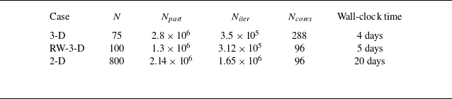
 N
 Npart
 Niter
 Ncores
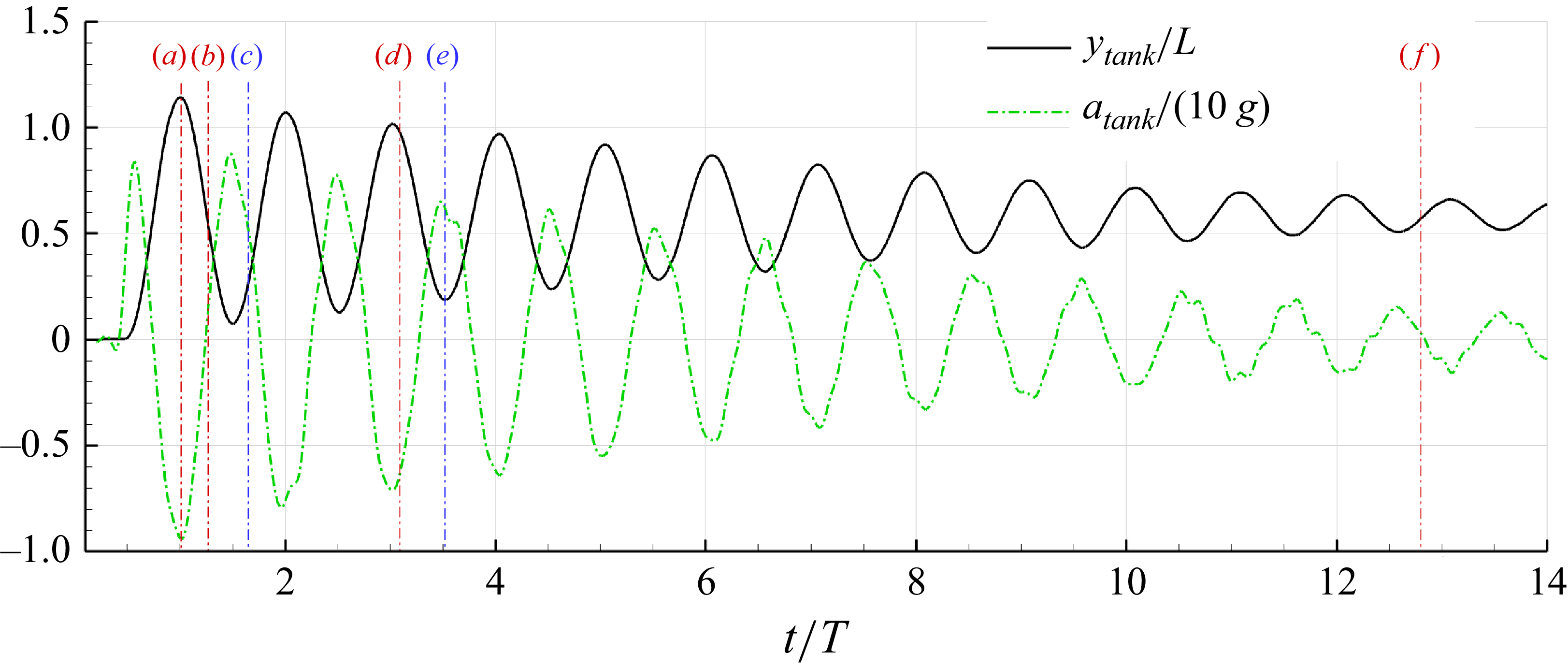

 t=0
 t=T
 t=1.5T
 t=2T
 t=18T
 t=24.13T

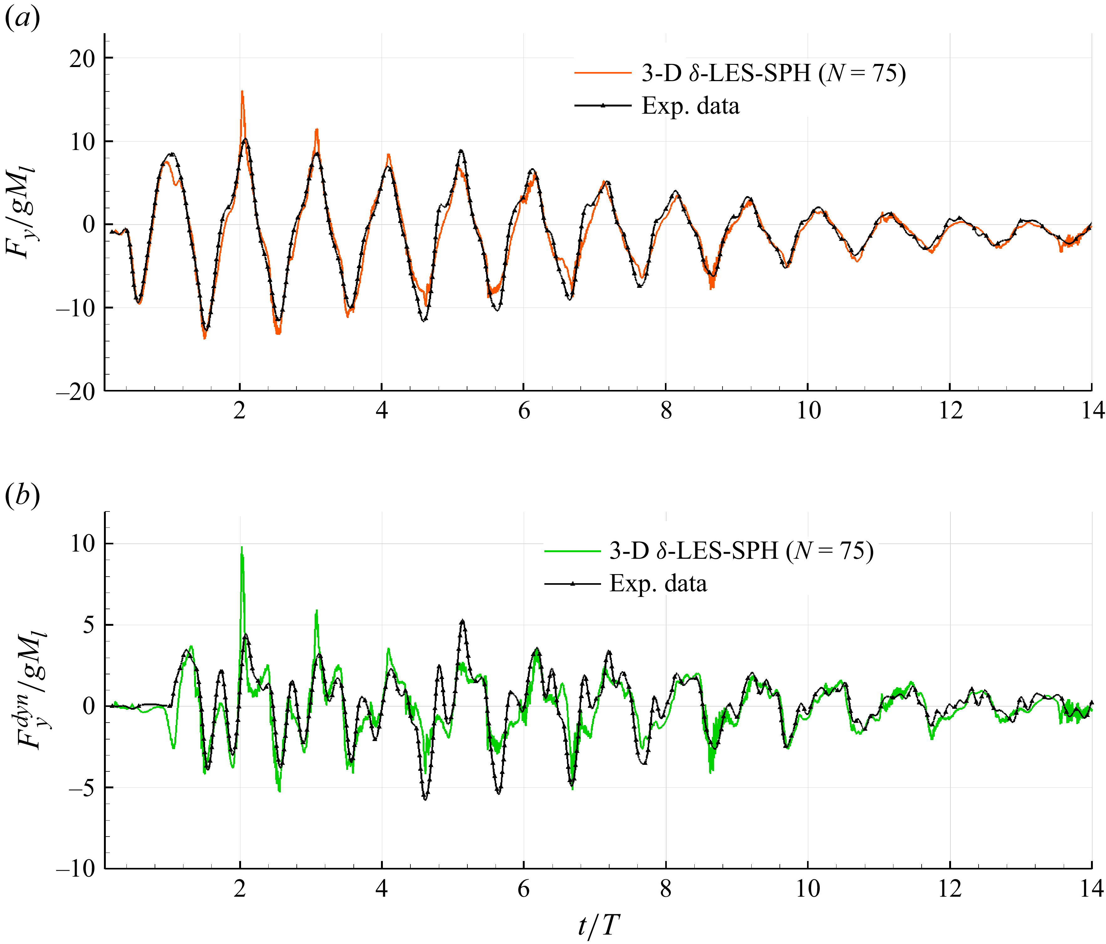
 δ
 Fydyn
 N=75

 δ
 Q
 Q=50Ω2
 t=1.65T
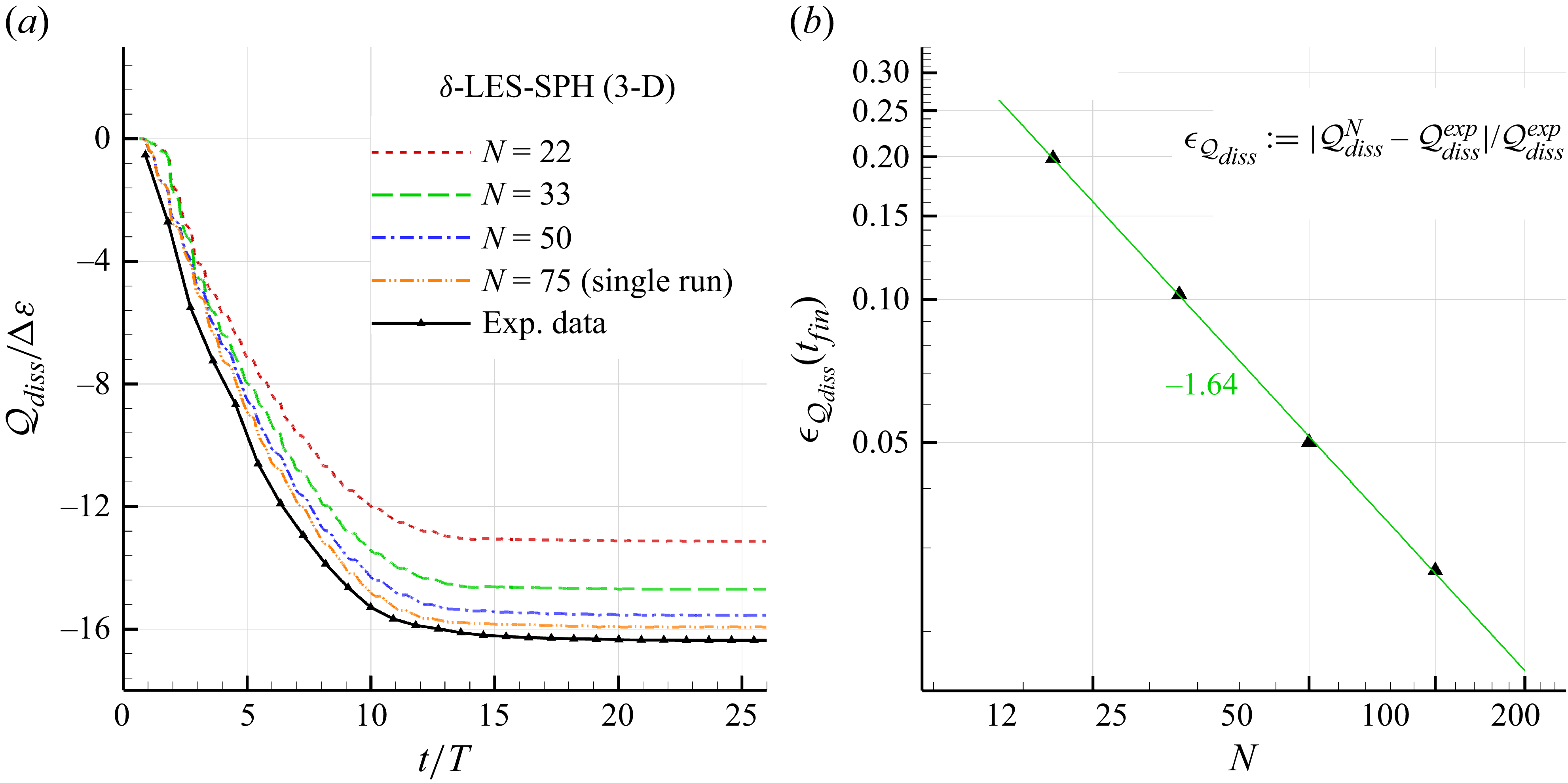
 Qdiss
 δ
 N

 δ
 Q
 t=1.65T
 z=W/6
 N=75
 N=800

 δ
 Q
 Q=100Ω2
 t=2.58T
 t=3.63T
 N=100

 δ
 N=50
 N=100
 N=75
 Q
 z=W/8
 N=100
 t=1.65T

 δ

 δ
 N=800

 δ
 Fydyn
 N=800

 δ
 Pdiss

 N=800
 N=75

 δ
 t=3.52T
 N=800
 μT

 δ
 Q
 t=3.52T

 Q
 50Ω2
 l=4Δr

 64
 8×8
 Re=106
 tU/L


 δ
 We=2240

 δ
 N=800
 t=3.67T
 We=2240

 δ
 Q
 t=3.67T
 We=2240

 Q
 50Ω2
 We=2240
 t=3.67T
 dQ
 l=4Δr
 We=2240
 We=∞
 λ/l

 δ

 δ
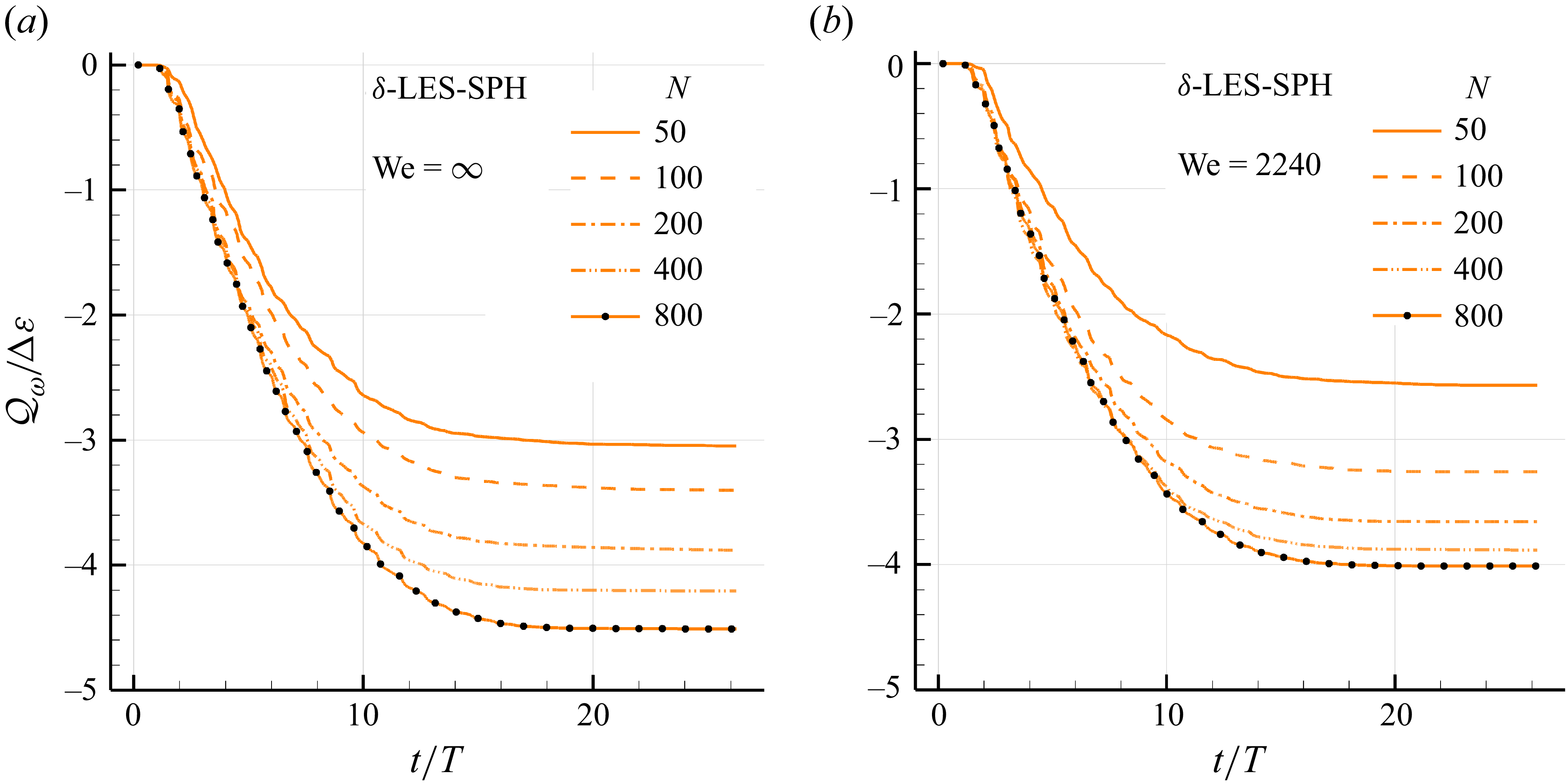
 Qω
 δ
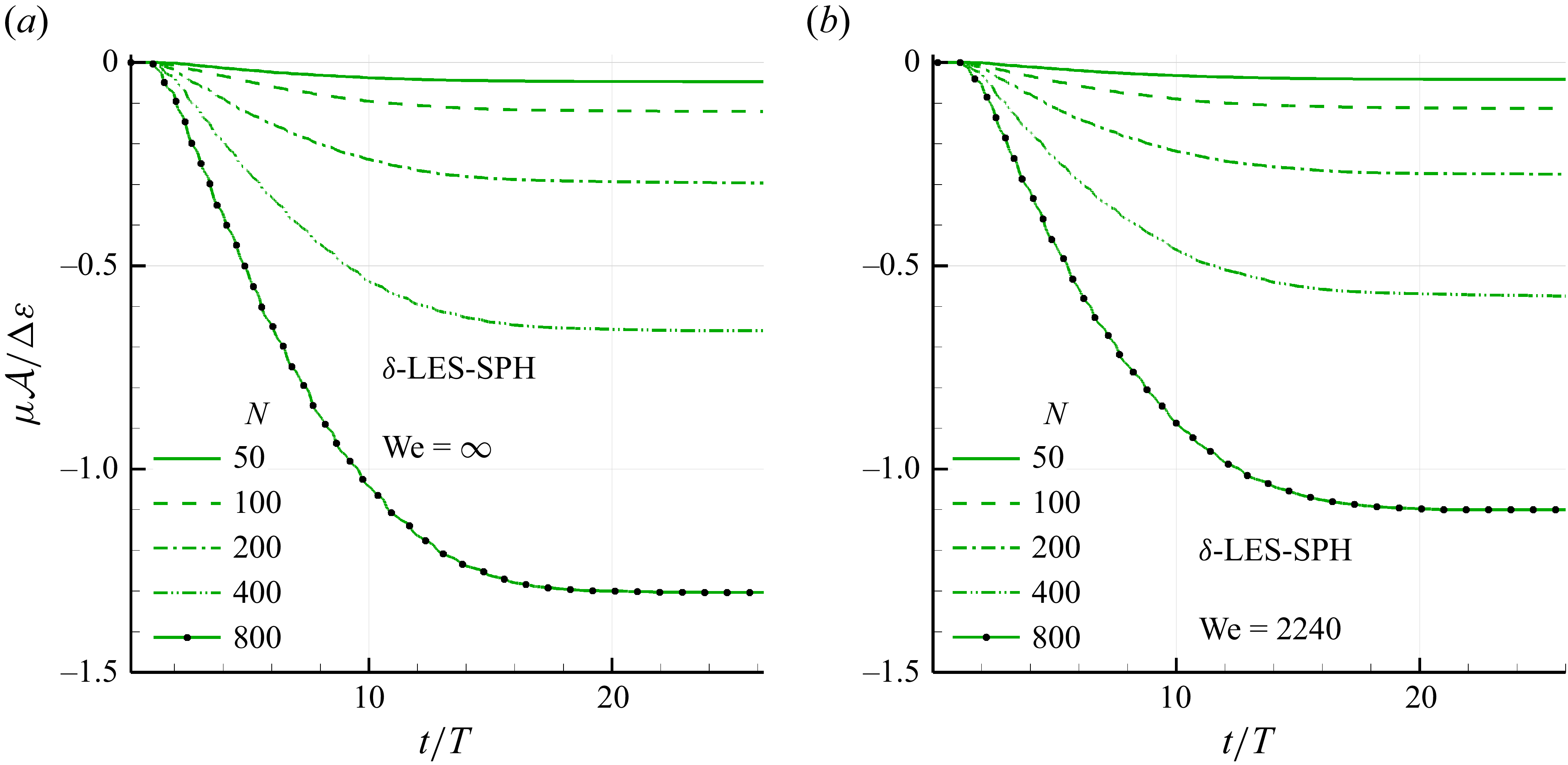
 A
 δ
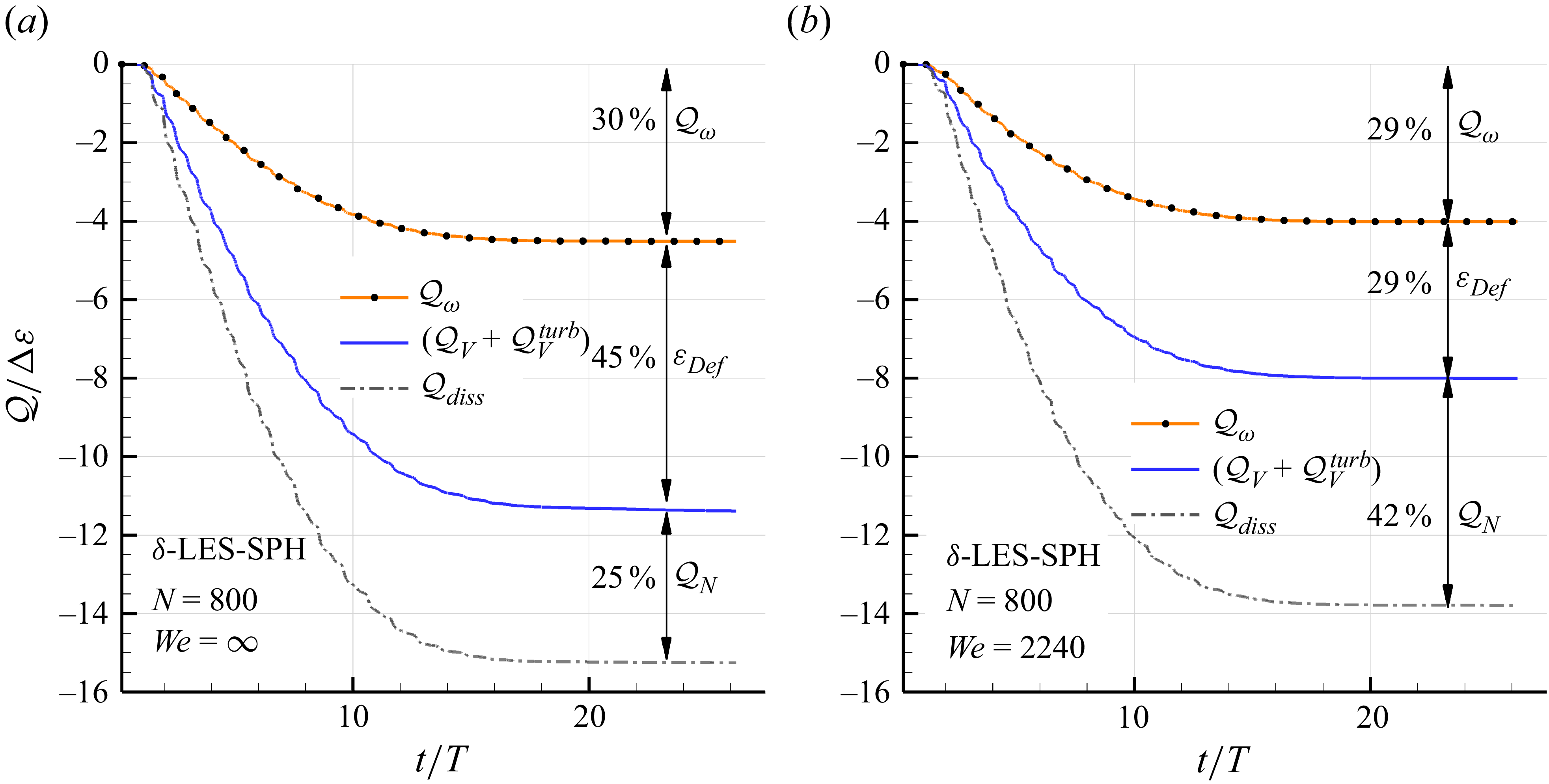
 N=800

 Qdiss
 δ
 We=∞

 Open access

