1 Introduction
Labs-on-a-chip (LOCs) are essential devices that are used for drug delivery, DNA analysis/sequencing systems, and biological/chemical agent detection sensors (Stone, Stroock & Ajdari Reference Stone, Stroock and Ajdari2004; Karniadakis, Beskok & Aluru Reference Karniadakis, Beskok and Aluru2005). Mixing and separating chemical species are two main processes that are performed in LOCs. In the first case, diffusion and dispersion are desirable, whereas in the second case they are unwanted mechanisms. In this sense, there are many ways to achieve mixing, such as molecular diffusion, eddy diffusion, advection, and Taylor dispersion. In particular, advection is the transport phenomenon that can produce chaotic advection when a stable and laminar flow exists, which could be useful for micromixing tasks. In this context, Taylor dispersion is due to the combined effects of advection and diffusion that are caused by velocity gradients. Meanwhile, electro-osmosis is used for transporting fluids through conduits of microscale size; however, that flow exhibits a plug-like velocity profile when the thickness of the EDL is very small relative to the diameter or height of the microchannels, thus diminishing the corresponding Taylor dispersion and limiting the micromixing. Based on the above discussion, one way to control Taylor dispersion in microchannels is by modifying the geometry of the microchannels (Datta & Ghosal Reference Datta and Ghosal2008) or by generating a disturbance in the flow. The latter effect could be achieved by modifying the wall
 $\unicode[STIX]{x1D701}$
potentials (Herr et al.
Reference Herr, Molho, Santiago, Mungal and Kenny2000; Ng & Zhou Reference Ng and Zhou2012a
,Reference Ng and Zhou
b
; Ng & Chen Reference Ng and Chen2013; Ng & Qi Reference Ng and Qi2014) or by temperature gradients (Tripathi, Bozkurt & Chauhan Reference Tripathi, Bozkurt and Chauhan2005; Kwak et al.
Reference Kwak, Kim, Hyun and Song2009; Bautista et al.
Reference Bautista, Sánchez, Arcos and Méndez2013; Vargas et al.
Reference Vargas, Arcos, Bautista and Méndez2017). One way to control the
 $\unicode[STIX]{x1D701}$
potential in the walls is by using field effects, which are achieved by using shielding electrodes in the channel walls, in the same manner as how field-effect transistors work (Schasfoort et al.
Reference Schasfoort, Schlautmann, Hendrikse and van den Berg1999; Lee et al.
Reference Lee, Lee, Fu, Lee and Yang2004a
; Chang & Yeo Reference Chang and Yeo2010; Nguyen Reference Nguyen2012). Therefore, the
 $\unicode[STIX]{x1D701}$
potential can be modified by controlling the shielding electrodes. Additionally, the
 $\unicode[STIX]{x1D701}$
potential can be changed by placing heterogeneous surface
 $\unicode[STIX]{x1D701}$
potential patches (Cho, Ho & Chen Reference Cho, Ho and Chen2010).
In recent years, both experimental and theoretical efforts (including those with advanced numerical methods such as molecular dynamics) have evaluated the effects of non-uniform wall charge,
 $\unicode[STIX]{x1D701}$
potential and surface modification in microfluidics and nanofluidics by means of electrostatic fields (Karnik & Castelino Reference Karnik and Castelino2006; Karnik et al.
Reference Karnik, Castelino, Fan, Yang and Majumdar2005a
,Reference Karnik, Fan, Yue, Li, Yang and Majumdar
b
, Reference Karnik, Duan, Castelino, Daiguji and Majumdar2007; Prakash, Karacor & Banerjee Reference Prakash, Karacor and Banerjee2009; Prakash & Karacor Reference Prakash and Karacor2011), by negatively charged substrates with discontinuous counter-charged patches (Zambrano et al.
Reference Zambrano, Pinti, Conlisk and Prakash2012), by an asymmetric surface charge (Prakash et al.
Reference Prakash, Zambrano, Fuest, Boone, Kim, Vasquez and Conlisk2015), using a three-state nanofluidic field switch (Fuest et al.
Reference Fuest, Boone, Rangharajan, Conlisk and Prakash2015), with an external field to manipulate the wall
 $\unicode[STIX]{x1D701}$
potential (Prakash & Conlisk Reference Prakash and Conlisk2016), and utilizing a gate electrode that modifies the modulation of the local surface potential (Fuest et al.
Reference Fuest, Rangharajan, Boone, Conlisk and Prakash2017).
The dispersion coefficient for an arbitrary uniform
 $\unicode[STIX]{x1D701}$
potential, electrolyte type, and cross-section geometry has been extensively studied (Zholkovskij, Masliyah & Czarnecki Reference Zholkovskij, Masliyah and Czarnecki2003; Zholkovskij & Masliyah Reference Zholkovskij and Masliyah2004). Datta & Ghosal (Reference Datta and Ghosal2009) argued that incidental/intentional variations in conditions such as the wall
 $\unicode[STIX]{x1D701}$
potential, cross-sectional area or the conductivity of the solution can induce pressure gradients in the EOF, making the flow non-uniform, contributing to hydrodynamic dispersion (Molho et al.
Reference Molho, Herr, Mosier, Santiago, Kenny, Brennen and Mohammadi2001; Ghosal Reference Ghosal2002, Reference Ghosal2003). Transporting of a solute in an axially variable flow and cross-sectional geometry was studied by Datta & Ghosal (Reference Datta and Ghosal2008). Nonlinear effects such as variable electric field, non-uniform
 $\unicode[STIX]{x1D701}$
potentials were addressed in determining the dispersion coefficient (Paul & Ng Reference Paul and Ng2012; Ng & Zhou Reference Ng and Zhou2012a
).
To improve the mixing process in microfluidic devices, electrokinetics pertaining to non-Newtonian fluids by generation disturbances in the flow has been analysed theoretically (Zhao et al. Reference Zhao, Zholkovskij, Masliyah and Yang2008; Vasu & De Reference Vasu and De2010; Hadigol et al. Reference Hadigol, Nosrati, Nourbakhsh and Raisee2011; Cho, Chen & Chen Reference Cho, Chen and Chen2012a ,Reference Cho, Chen and Chen b ; Ng & Qi Reference Ng and Qi2014). Recently, studies in EOFs of viscoelastic fluids has been necessary due to their direct application in biological systems, separation of heavy protein molecules, and the mixing of chemical reagents (Afonso, Alves & Pinho Reference Afonso, Alves and Pinho2009; Ferrás et al. Reference Ferrás, Afonso, Alves, Nóbrega and Pinho2014; Ghosh & Chakraborty Reference Ghosh and Chakraborty2015).
Because we will address the hydrodynamic dispersion of a neutral solute in an EOF in a viscoelastic fluid in terms of the Van Deemter (Deemter, Zuiderweg & Klinkenberg Reference Deemter, Zuiderweg and Klinkenberg1956) equation, we first present some antecedents that allow identifying the importance of our work, which concerns the dispersion coefficient. Band broadening on the hydrodynamic dispersion mechanics through a channel was first analysed by Taylor (Reference Taylor1953). Subsequently, Aris (Reference Aris1956, Reference Aris1959) introduced the effective diffusion constant as the sum of the axial molecular diffusion and the Taylor radial dispersion coefficients derived from the analysis of Taylor (Reference Taylor1953). In this context, the dispersion coefficient
 $K_{eff}$
for a flow of a general type of solute and for an arbitrary cross-section geometry under the simultaneous action of molecular diffusion
 $D$
and variation in the velocity over the cross-section of the solvent is derived as
 $$\begin{eqnarray}\displaystyle & \displaystyle K_{eff}=D\left[1+\left(\frac{\bar{u}H_{\ast }}{4D}\right)^{2}\right]. & \displaystyle\end{eqnarray}$$
The relationship (1.1) depends on the mean cross-sectional velocity
 $\bar{u}$
of the flow and on the parameter
 $H_{\ast }$
. The latter represents the minimum plate height, which depends on the cross-sectional geometry of the channel and on the hydrodynamics of the flow and, for convenience, will be defined in § 2.2. Dutta, Ramachandran & Leighton (Reference Dutta, Ramachandran and Leighton2006) introduced a factor
 $f$
in (1.1) that considers the aspect ratio for typical channel geometries on the hydrodynamic dispersion coefficient; in addition channels with triangular, parabolic, and elliptical cross-sections were reported (Ajdari, Bontoux & Stone Reference Ajdari, Bontoux and Stone2006).
For the case of a pure EOF in a slit microchannel with a Newtonian fluid and non-uniformity of the hydrodynamic flow within the channel cross-section, the dispersion coefficient (1.1) becomes (Griffiths & Nilson Reference Griffiths and Nilson1999)
 $$\begin{eqnarray}\displaystyle & \displaystyle K_{eff}=D\Bigg\{1+{\displaystyle \frac{1}{12}}\left(\frac{\unicode[STIX]{x1D716}E_{x}\unicode[STIX]{x1D701}}{\unicode[STIX]{x1D707}\unicode[STIX]{x1D705}D}\right)^{2}\left[1-{\displaystyle \frac{\tanh \unicode[STIX]{x1D705}h}{\unicode[STIX]{x1D705}h}}\right]^{2}f(\unicode[STIX]{x1D705}h)\Bigg\}. & \displaystyle\end{eqnarray}$$
In the above expression,
 $\unicode[STIX]{x1D716}$
is the dielectric constant of the electrolyte,
 $E_{x}$
represents the applied axial electric field,
 $\unicode[STIX]{x1D701}$
is the uniform electric potential on the channel wall, and
 $\unicode[STIX]{x1D707}$
and
 $D$
are the Newtonian fluid viscosity and the diffusion coefficient, respectively. The factor
 $f(\unicode[STIX]{x1D705}h)$
that appears in (1.2) only depends on the aspect ratio of the half-height of the microchannel
 $h$
and the inverse double layer thickness
 $\unicode[STIX]{x1D705}$
. If any of the parameters involved in (1.2) vary along the microchannel, then the EOF is perturbed and pressure gradients will be induced, causing a non-uniform flow along the microchannel. Here, we are interested in determining the effects that the non-uniformity of the
 $\unicode[STIX]{x1D701}$
potential and the fluid rheology (according to the simplified Phan-Thien–Tanner (sPTT) model) have on the dispersion coefficient.
To conduct the theoretical analysis of the dispersion coefficient explained previously, we assume that the microchannel walls have sinusoidally modulated low
 $\unicode[STIX]{x1D701}$
potentials that vary slowly in the axial direction (see Ng & Zhou Reference Ng and Zhou2012a
; Ng & Qi Reference Ng and Qi2014; Ghosh & Chakraborty Reference Ghosh and Chakraborty2015; Qi & Ng Reference Qi and Ng2015); additionally, we analysed the stage when the
 $\unicode[STIX]{x1D701}$
potential is increased uniformly. To obtain approximate analytical solutions for the dimensionless EDL potential, the Poisson–Boltzmann equation was simplified using the Debye–Hückel approximation (Masliyah & Bhattacharjee Reference Masliyah and Bhattacharjee2006); therefore, the wall potentials are considered to be small enough so that the Debye–Hückel approximation remains valid. The flow field and the dispersion coefficient were solved in the limit of the lubrication approximation theory (LAT) (Ghosal Reference Ghosal2002; Bautista et al.
Reference Bautista, Sánchez, Arcos and Méndez2013) using regular perturbation techniques (Bender & Orszag Reference Bender and Orszag1999).
Our analysis reveals that an imposed axially slowly varying
 $\unicode[STIX]{x1D701}$
potential significantly alters the hydrodynamic dispersion coefficient for viscoelastic fluids compared to a Newtonian fluid, and this contrast is more significant for values of the Deborah number, defined below, of order unity.
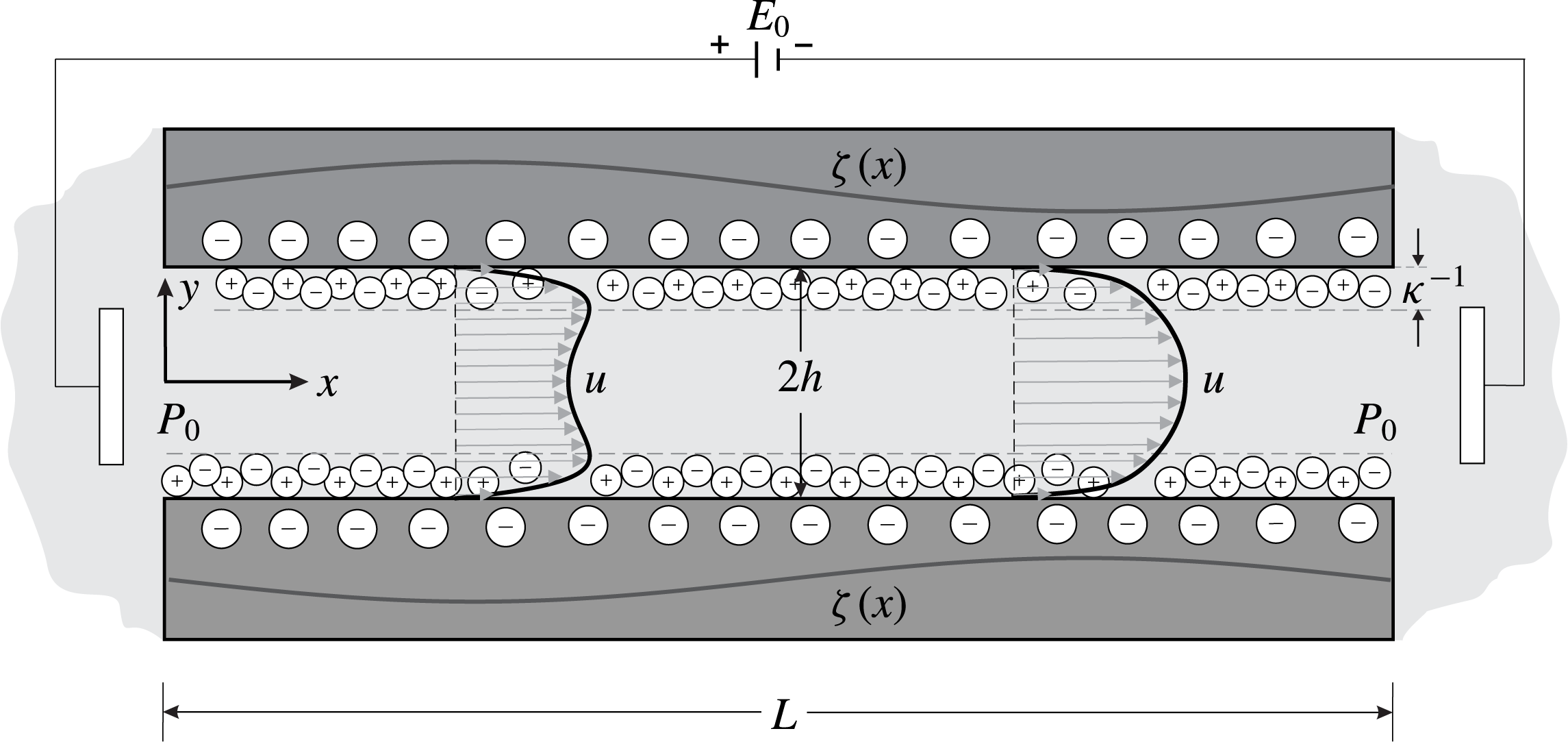
Schematic diagram of the studied physical model.

The remainder of this paper is organized as follows. In § 2, the physical problem and the main considerations are described. In § 3, the governing equations and the corresponding boundary conditions are presented. Next, in § 4, the governing equations are formulated in the dimensionless forms. An asymptotic solution to the dimensionless governing equations is provided in detail in § 5. Finally, the main results are discussed in § 6.
2 Formulation
2.1 Physical model
The sketch of the physical model studied in this work is shown in figure 1. The transport of a neutral solute through a narrow channel in an EOF of a viscoelastic fluid is considered. The half-thickness of the microchannel is
 $h$
and its length is denoted by
 $L$
, where
 $L\gg h$
. For convenience, the origin of the Cartesian coordinate system is placed at the left end and middle plane of the microchannel, with the
 $x$
-coordinate in the direction of motion and the
 $y$
-coordinate normal to the microchannel walls. We consider that the walls of the microchannel have sinusoidally modulated low
 $\unicode[STIX]{x1D701}$
potentials, which vary slowly in the
 $x$
direction. According to previous studies (Anderson & Idol Reference Anderson and Idol1985; Ghosal Reference Ghosal2002; Datta, Ghosal & Patankar Reference Datta, Ghosal and Patankar2006; Ng & Zhou Reference Ng and Zhou2012a
), the analysis is conducted by considering that the wall
 $\unicode[STIX]{x1D701}$
potential changes by the following relationship:
 $$\begin{eqnarray}\displaystyle & \displaystyle \unicode[STIX]{x1D701}(x)=\unicode[STIX]{x1D701}_{0}+\unicode[STIX]{x0394}\unicode[STIX]{x1D701}\unicode[STIX]{x1D70E}_{1}\sin \left(\frac{2\unicode[STIX]{x03C0}x}{L}+\unicode[STIX]{x1D70E}_{2}\right), & \displaystyle\end{eqnarray}$$
where
 $\unicode[STIX]{x1D701}_{0}$
is the value of a reference
 $\unicode[STIX]{x1D701}$
potential and
 $\unicode[STIX]{x0394}\unicode[STIX]{x1D701}$
, which is smaller than
 $\unicode[STIX]{x1D701}_{0}$
, is the amplitude of the fluctuations on
 $\unicode[STIX]{x1D701}(x)$
. The parameter
 $\unicode[STIX]{x1D70E}_{1}$
is the amplitude, and
 $\unicode[STIX]{x1D70E}_{2}$
represents a phase lag of the sine function in (2.1). In the analysis, the values of
 $(\unicode[STIX]{x1D70E}_{1},\unicode[STIX]{x1D70E}_{2})=(1,0)$
represent the sine function of the variation in
 $\unicode[STIX]{x1D701}(x)$
and provide a qualitative overview of how the electrokinetic flow might depend on the amplitude and length scale of any fluctuation in
 $x$
. To appreciably enhance the local dispersion coefficient, we have considered values for the amplitude and phase lag of
 $(\unicode[STIX]{x1D70E}_{1},\unicode[STIX]{x1D70E}_{2})=(\sqrt{2},\unicode[STIX]{x03C0}/4)$
in (2.1) (Goodwine Reference Goodwine2011).
The microchannel ends have the same pressure
 $p=P_{0}$
. The flow is driven by electro-osmotic forces, originating from the simultaneous effect of an external electric field of strength
 $E_{0}=\unicode[STIX]{x1D719}_{0}/L$
and the induced electric field in the EDL. Here,
 $\unicode[STIX]{x1D719}_{0}$
is the electric potential imposed at the inlet of the microchannel. In addition, the assumptions to be taken into account in the analysis are the following. (i) The flow is considered to be at steady state, laminar and incompressible. (ii) The parameter
 $\unicode[STIX]{x1D6FD}=h/L$
and the Reynolds number
 $Re$
, defined below, are typically very small relative to unity (Ghosal Reference Ghosal2002), i.e.
 $\unicode[STIX]{x1D6FD}\sim 10^{-3}$
and
 $Re\sim 10^{-3}{-}10^{-1}$
. (iii) The fluid is a symmetric electrolyte solution
 $(z:z)$
, where
 $z$
is the absolute value of the valency, and the potential distribution
 $\unicode[STIX]{x1D713}$
into the EDL is described by the Poisson–Boltzmann equation. (iv) The axial variation of the electric potential,
 $\unicode[STIX]{x1D719}_{0}/L$
, is considerably smaller than the transverse variation of the potential into the EDL,
 $\unicode[STIX]{x1D701}_{0}/\unicode[STIX]{x1D706}_{D}$
, where
 $\unicode[STIX]{x1D706}_{D}=(\unicode[STIX]{x1D716}k_{B}T/2z^{2}e^{2}n_{\infty })^{1/2}$
is the double layer thickness, also denoted by
 $\unicode[STIX]{x1D705}^{-1}$
. Here,
 $e$
represents the fundamental charge of an electron,
 $n_{\infty }$
is the ionic number in the concentration in the bulk solution,
 $k_{B}$
is the Boltzmann constant, and
 $T$
is the absolute temperature. (v) The Debye–Hückel approximation is assumed, which is valid for low
 $\unicode[STIX]{x1D701}$
potentials, i.e.
 $\unicode[STIX]{x1D701}_{0}<25$
mV (see Burgreen & Nakache Reference Burgreen and Nakache1964; Rice & Whitehead Reference Rice and Whitehead1965; Levine, Marriott & Neale Reference Levine, Marriott and Neale1975; Probstein Reference Probstein2003). (vi) The microchannel wall
 $\unicode[STIX]{x1D701}(x)$
potentials vary slowly and sinusoidally according to the relationship given in (2.1). (vii) Finally, due to the symmetry, the half-height of the microchannel is considered for the analysis.
2.2 Hydrodynamic dispersion coefficient
Let us consider the hydrodynamic dispersion that occurs due to the non-uniformity of the velocity due to the
 $\unicode[STIX]{x1D701}$
potential variation in a pure EOF through a straight microchannel. For a general type of flow, when diffusional and hydrodynamic dispersions are present, by following the analyses performed by Datta & Ghosal (Reference Datta and Ghosal2009), Ng & Chen (Reference Ng and Chen2013) and Zholkovskij, Masliyah & Yaroshchuk (Reference Zholkovskij, Masliyah and Yaroshchuk2013), the dispersion coefficient,
 $K_{eff}$
, describes the rate of the change of the statical variance
 $\unicode[STIX]{x1D70E}^{2}$
with time. It is defined as (Aris Reference Aris1956)
 $$\begin{eqnarray}\displaystyle & \displaystyle K_{eff}=\frac{1}{2}\frac{\text{d}\unicode[STIX]{x1D70E}^{2}(t)}{\text{d}t}. & \displaystyle\end{eqnarray}$$
The variance
 $\unicode[STIX]{x1D70E}^{2}$
characterizes the shape of the solute distribution band at a given instant. Another parameter, which describes changes in the variance
 $\unicode[STIX]{x1D70E}^{2}$
during the band displacement at the unit distance, is referred to as the plate height,
 $H$
,
 $$\begin{eqnarray}\displaystyle & \displaystyle H=\frac{\text{d}\unicode[STIX]{x1D70E}^{2}(x_{c})}{\text{d}x_{c}}. & \displaystyle\end{eqnarray}$$
Thus, (2.2) and (2.3) define the major parameters employed in the literature for describing the band broadening. In addition to a given bandwidth from the band variance
 $\unicode[STIX]{x1D70E}$
as a function of time
 $t$
and the band centre of mass
 $x_{c}$
, it is convenient to characterize the velocity of the centre of mass to assess the hydrodynamic dispersion coefficient
 $K_{eff}$
. In this case, for a band of a non-adsorbing solute flowing through a straight channel, the centre-of-mass velocity coincides with the cross-sectional mean velocity
 $\bar{u}$
:
 $$\begin{eqnarray}\displaystyle & \displaystyle \bar{u}=\frac{\text{d}x_{c}}{\text{d}t}. & \displaystyle\end{eqnarray}$$
By combining (2.2)–(2.4), we obtain
 $$\begin{eqnarray}\displaystyle & \displaystyle K_{eff}={\textstyle \frac{1}{2}}\bar{u}H, & \displaystyle\end{eqnarray}$$
where the cross-sectional mean velocity of the velocity flow
 $u(x,y)$
in the
 $x$
direction is defined as
 $$\begin{eqnarray}\displaystyle & \displaystyle \bar{u}=\frac{1}{h}\int _{0}^{h}u\left(x,y\right)\,\text{d}y, & \displaystyle\end{eqnarray}$$
and
 $H$
is the plate height, estimated from the classical Van Deemter (Deemter et al.
Reference Deemter, Zuiderweg and Klinkenberg1956) equation:
 $$\begin{eqnarray}\displaystyle & \displaystyle H=\frac{2D}{\bar{u}}+\frac{\bar{u}}{8D}H_{\ast }^{2}. & \displaystyle\end{eqnarray}$$
In the above equation,
 $D$
denotes the molecular coefficient and
 $H_{\ast }$
is the minimum plate height, which is evaluated from the following expression (Zholkovskij et al.
Reference Zholkovskij, Masliyah and Yaroshchuk2013):
 $$\begin{eqnarray}\displaystyle & \displaystyle H_{\ast }^{2}=\frac{16}{h}\int _{0}^{h}\left[\int _{0}^{y}\left(\frac{u}{\bar{u}}-1\right)\,\text{d}y\right]^{2}\,\text{d}y. & \displaystyle\end{eqnarray}$$
Finally, after combining (2.5) and (2.7), the hydrodynamic dispersion coefficient is obtained by (1.1). From another perspective (Ng & Chen Reference Ng and Chen2013; Hoshyargar, Ashrafizadeh & Sadeghi Reference Hoshyargar, Ashrafizadeh and Sadeghi2017), an equivalent expression to (2.5) for determining
 $K_{eff}$
can be obtained by applying the homogenization method to the convection–diffusion equation with no reaction (Mei & Vernescu Reference Mei and Vernescu2010; Mei, Auriault & Ng Reference Mei, Auriault and Ng1996). In the following section, we present the governing equations that allow us to determine the EOF field for a viscoelastic fluid in a microchannel with varying wall
 $\unicode[STIX]{x1D701}(x)$
potentials that are needed to determine the effective dispersion coefficient (2.5).
3 Governing equations
3.1 Flow field governing equations
The basic equations that will form the starting point for studying the steady-state two-dimensional pure EOF of a viscoelastic fluid are the continuity equation,
 $$\begin{eqnarray}\displaystyle & \displaystyle \unicode[STIX]{x1D735}\boldsymbol{\cdot }\boldsymbol{u}=0, & \displaystyle\end{eqnarray}$$
and the modified Cauchy equation of motion, which is given by
 $$\begin{eqnarray}\displaystyle & \displaystyle \unicode[STIX]{x1D70C}\left(\boldsymbol{u}\boldsymbol{\cdot }\unicode[STIX]{x1D735}\boldsymbol{u}\right)=-\unicode[STIX]{x1D735}p+\unicode[STIX]{x1D735}\boldsymbol{\cdot }\boldsymbol{\unicode[STIX]{x1D70F}}+\unicode[STIX]{x1D70C}_{e}\boldsymbol{E}. & \displaystyle\end{eqnarray}$$
Here,
 $\unicode[STIX]{x1D70C}$
is the mass density of the fluid,
 $p$
is the pressure and
 $\boldsymbol{\unicode[STIX]{x1D70F}}$
is the polymeric extra-stress contribution.
 $\unicode[STIX]{x1D70C}_{e}$
defines the electric charge density per unit volume in the EDL (Chang & Yeo Reference Chang and Yeo2010), and
 $\boldsymbol{E}=-\unicode[STIX]{x1D735}\unicode[STIX]{x1D6F7}$
is the electric field vector, where
 $\unicode[STIX]{x1D6F7}$
represents the total electric potential in the microchannel, which will be described in detail in § 3.2. Furthermore, the nabla operator is defined as
 $\unicode[STIX]{x1D735}\equiv (\unicode[STIX]{x2202}/\unicode[STIX]{x2202}x\quad \boldsymbol{i},\unicode[STIX]{x2202}/\unicode[STIX]{x2202}y\quad \boldsymbol{j})$
, where
 $\boldsymbol{i}$
and
 $\boldsymbol{j}$
are the standard unit vectors.
The hydrodynamic boundary conditions related to the impermeability and no-slip on the walls of the microchannel are given by
 $$\begin{eqnarray}\displaystyle & \displaystyle \boldsymbol{u}\boldsymbol{\cdot }\boldsymbol{n}=\mathbf{0} & \displaystyle\end{eqnarray}$$
and
 $$\begin{eqnarray}\displaystyle & \displaystyle \boldsymbol{u}-(\boldsymbol{u}\boldsymbol{\cdot }\boldsymbol{n})\boldsymbol{n}=\mathbf{0}, & \displaystyle\end{eqnarray}$$
respectively. Additionally, the symmetry boundary condition at the midplane of the microchannel requires that
 $\boldsymbol{\unicode[STIX]{x1D70F}}=\mathbf{0}$
, and we consider that the pressure is
 $P_{0}$
at
 $x=0$
and at
 $x=L$
. The unit normal vector at the plate surface is
 $\boldsymbol{n}=\{0,1\}$
.
3.1.1 sPTT constitutive fluid model
The sPTT model involved in the modified momentum (3.2) is given by (Thien & Tanner Reference Thien and Tanner1977)
 $$\begin{eqnarray}\displaystyle & \displaystyle \unicode[STIX]{x1D706}\frac{\unicode[STIX]{x1D63F}\boldsymbol{\unicode[STIX]{x1D70F}}}{\unicode[STIX]{x1D63F}t}+\unicode[STIX]{x1D64D}=\mathbf{0}. & \displaystyle\end{eqnarray}$$
In the above relationship,
 $t$
and
 $\unicode[STIX]{x1D706}$
are the time and relaxation time, respectively.
 $\unicode[STIX]{x1D63F}\boldsymbol{\unicode[STIX]{x1D70F}}/\unicode[STIX]{x1D63F}t$
is the upper convective derivative, defined as
 $$\begin{eqnarray}\displaystyle & \displaystyle \frac{\unicode[STIX]{x1D63F}\boldsymbol{\unicode[STIX]{x1D70F}}}{\unicode[STIX]{x1D63F}t}=\boldsymbol{u}\boldsymbol{\cdot }\unicode[STIX]{x1D735}\boldsymbol{\unicode[STIX]{x1D70F}}-\unicode[STIX]{x1D647}\boldsymbol{\unicode[STIX]{x1D70F}}-\boldsymbol{\unicode[STIX]{x1D70F}}\unicode[STIX]{x1D647}^{\text{T}}, & \displaystyle\end{eqnarray}$$
and
 $\unicode[STIX]{x1D64D}$
is given by
 $$\begin{eqnarray}\displaystyle & \displaystyle \unicode[STIX]{x1D64D}=\left\{1+\tilde{\unicode[STIX]{x1D716}}\frac{\unicode[STIX]{x1D706}}{\unicode[STIX]{x1D702}}\text{tr}(\boldsymbol{\unicode[STIX]{x1D70F}})\right\}\boldsymbol{\unicode[STIX]{x1D70F}}-2\unicode[STIX]{x1D702}\unicode[STIX]{x1D63F}. & \displaystyle\end{eqnarray}$$
Here,
 $\unicode[STIX]{x1D702}$
is a constant viscosity coefficient, and
 $\tilde{\unicode[STIX]{x1D716}}$
is a parameter that governs the extensional flow response;
 $\text{tr}(\boldsymbol{\unicode[STIX]{x1D70F}})$
is the trace of
 $\boldsymbol{\unicode[STIX]{x1D70F}}$
, and
 $\unicode[STIX]{x1D63F}$
is the rate-of-strain tensor, which is defined as
 $$\begin{eqnarray}\displaystyle & \displaystyle \unicode[STIX]{x1D63F}={\textstyle \frac{1}{2}}\left(\unicode[STIX]{x1D647}+\unicode[STIX]{x1D647}^{\text{T}}\right), & \displaystyle\end{eqnarray}$$
where
 $\unicode[STIX]{x1D647}=\unicode[STIX]{x2202}u_{i}/\unicode[STIX]{x2202}x_{j}$
is the tensor of the velocity gradient, and
 $u_{i}$
are the corresponding components of the velocity vector field
 $\boldsymbol{u}$
. The superscript
 $T$
denotes the transpose of
 $\unicode[STIX]{x1D647}$
.
3.2 Electric field
To define the interaction between the total electric potential
 $\unicode[STIX]{x1D6F7}$
and the ion concentration, at any position in the microchannel, we use the Poisson equation (Newman & Thomas-Alyea Reference Newman and Thomas-Alyea2004),
 $$\begin{eqnarray}\displaystyle & \displaystyle \unicode[STIX]{x1D6FB}^{2}\unicode[STIX]{x1D6F7}=-\frac{\unicode[STIX]{x1D70C}_{e}}{\unicode[STIX]{x1D716}}. & \displaystyle\end{eqnarray}$$
In accordance with assumption (iii) in § 2, the electric charge density follows the Boltzmann distribution (Masliyah & Bhattacharjee Reference Masliyah and Bhattacharjee2006), which is given by
 $$\begin{eqnarray}\displaystyle & \displaystyle \unicode[STIX]{x1D70C}_{e}=-2zen_{\infty }\sinh \left(\frac{ze\unicode[STIX]{x1D713}}{k_{B}T}\right). & \displaystyle\end{eqnarray}$$
It is reasonable to assume that the electric potential,
 $\unicode[STIX]{x1D6F7}$
, can be expressed by the linear superposition of the EDL potential and the externally applied potential,
 $\unicode[STIX]{x1D719}(x)$
, valid for long microchannels. By neglecting any end effects, one can write
 $\unicode[STIX]{x1D6F7}(x,y)=\unicode[STIX]{x1D713}(y)+\unicode[STIX]{x1D719}(x)$
. For a long microchannel,
 $L\gg h$
; therefore, the term
 $\unicode[STIX]{x2202}^{2}\unicode[STIX]{x1D6F7}/\unicode[STIX]{x2202}x^{2}$
in (3.9) may be neglected (Probstein Reference Probstein2003), leading to
 $$\begin{eqnarray}\displaystyle & \displaystyle \frac{\text{d}^{2}\unicode[STIX]{x1D713}}{\text{d}y^{2}}=\unicode[STIX]{x1D705}^{2}\unicode[STIX]{x1D713}. & \displaystyle\end{eqnarray}$$
From the above equation and the boundary conditions
 $\text{d}\unicode[STIX]{x1D713}/\text{d}y=0$
at
 $y=0$
and
 $\unicode[STIX]{x1D713}=\unicode[STIX]{x1D701}(x)$
at
 $y=h$
, the well-known solution for the distribution of the potential,
 $\unicode[STIX]{x1D713}$
, with a free charge density defined as
 $\unicode[STIX]{x1D70C}_{e}=-\unicode[STIX]{x1D716}\unicode[STIX]{x1D705}^{2}\unicode[STIX]{x1D713}$
is given by
 $\unicode[STIX]{x1D713}=\unicode[STIX]{x1D701}(x)\cosh \unicode[STIX]{x1D705}y/\cosh \unicode[STIX]{x1D705}h$
. The modulations in
 $\unicode[STIX]{x1D701}(x)$
obey the equations presented in (2.1).
4 Formulation of the dimensionless problem
We introduce the following dimensionless variables:
 $\tilde{x}=x/L$
,
 ${\tilde{y}}=y/h$
,
 $\tilde{u} =u/U_{HS}$
,
 $\tilde{v}=vL/U_{HS}h$
,
 $\tilde{p}=(p^{\prime }-P_{0})h^{2}/\unicode[STIX]{x1D702}U_{HS}L$
,
 $\tilde{\boldsymbol{\unicode[STIX]{x1D70F}}}=\boldsymbol{\unicode[STIX]{x1D70F}}h/\unicode[STIX]{x1D702}U_{HS}$
, and
 $\tilde{\unicode[STIX]{x1D713}}=\unicode[STIX]{x1D713}/\unicode[STIX]{x1D701}_{0}$
. Here,
 $U_{HS}=-\unicode[STIX]{x1D716}\unicode[STIX]{x1D701}_{0}E_{0}/\unicode[STIX]{x1D702}$
is the Helmholtz–Smoluchowski velocity, and the stress tensor has the components
 $\boldsymbol{\unicode[STIX]{x1D70F}}=\boldsymbol{\unicode[STIX]{x1D70F}}(\unicode[STIX]{x1D70F}_{xx},\unicode[STIX]{x1D70F}_{xy},\unicode[STIX]{x1D70F}_{yy})$
. When defining the dimensionless pressure
 $\tilde{p}$
, we have introduced the useful definition
 $p^{\prime }=p-\unicode[STIX]{x1D716}\unicode[STIX]{x1D705}^{2}\unicode[STIX]{x1D713}^{2}/2$
(Ajdari Reference Ajdari1995, Reference Ajdari1996). Next, we show the non-dimensional version of the governing equations presented in § 3.
4.1 Dispersion coefficient
Upon introducing the non-dimensional variables, the non-dimensional dispersion coefficient (2.5) becomes
 $$\begin{eqnarray}\displaystyle & \displaystyle \tilde{K}_{eff}=1+\left(\frac{Pe\,\tilde{\bar{u}}\tilde{H}_{\ast }}{4}\right)^{2}, & \displaystyle\end{eqnarray}$$
where
 $\tilde{K}_{eff}=K_{eff}/D$
,
 $Pe=U_{HS}h/D$
is the Péclet number,
 $\tilde{H}_{\ast }=H_{\ast }/h$
and
 $\tilde{\bar{u}}=\bar{u}/U_{HS}$
is the dimensionless cross-sectional mean velocity of the flow through the microchannel, which is evaluated by
 $$\begin{eqnarray}\displaystyle & \displaystyle \tilde{\bar{u}}=\int _{{\tilde{y}}=0}^{{\tilde{y}}=1}\tilde{u} \,\text{d}{\tilde{y}}. & \displaystyle\end{eqnarray}$$
The dimensionless minimum plate height,
 $\tilde{H}_{\ast }$
, can be written as
 $$\begin{eqnarray}\displaystyle & \displaystyle \tilde{H}_{\ast }^{2}=16\int _{0}^{1}\left[\int _{0}^{{\tilde{y}}}\left(\frac{\tilde{u} }{\tilde{\bar{u}}}-1\right)\,\text{d}{\tilde{y}}\right]^{2}\,\text{d}{\tilde{y}}. & \displaystyle\end{eqnarray}$$
Next, we present the non-dimensional problem that allows determination of the flow field.
4.2 Flow field
The dimensionless forms of governing equations (3.1) and (3.2) for a pure EOF are as follows:
 $$\begin{eqnarray}\displaystyle & \displaystyle \frac{\unicode[STIX]{x2202}\tilde{u} }{\unicode[STIX]{x2202}\tilde{x}}+\frac{\unicode[STIX]{x2202}\tilde{v}}{\unicode[STIX]{x2202}{\tilde{y}}}=0, & \displaystyle\end{eqnarray}$$
 $$\begin{eqnarray}\displaystyle & \displaystyle \unicode[STIX]{x1D6FD}Re\left(\tilde{u} \frac{\unicode[STIX]{x2202}\tilde{u} }{\unicode[STIX]{x2202}\tilde{x}}+\tilde{v}\frac{\unicode[STIX]{x2202}\tilde{u} }{\unicode[STIX]{x2202}{\tilde{y}}}\right)=-\frac{\unicode[STIX]{x2202}\tilde{P}}{\unicode[STIX]{x2202}\tilde{x}}+\unicode[STIX]{x1D6FD}\frac{\unicode[STIX]{x2202}\tilde{\unicode[STIX]{x1D70F}}_{xx}}{\unicode[STIX]{x2202}\tilde{x}}+\frac{\unicode[STIX]{x2202}\tilde{\unicode[STIX]{x1D70F}}_{yx}}{\unicode[STIX]{x2202}{\tilde{y}}}+\tilde{\unicode[STIX]{x1D705}}^{2}\tilde{\unicode[STIX]{x1D713}} & \displaystyle\end{eqnarray}$$
and
 $$\begin{eqnarray}\displaystyle & \displaystyle \unicode[STIX]{x1D6FD}^{3}Re\left(\tilde{u} \frac{\unicode[STIX]{x2202}\tilde{v}}{\unicode[STIX]{x2202}\tilde{x}}+\tilde{v}\frac{\unicode[STIX]{x2202}\tilde{v}}{\unicode[STIX]{x2202}{\tilde{y}}}\right)=-\frac{\unicode[STIX]{x2202}\tilde{P}}{\unicode[STIX]{x2202}{\tilde{y}}}+\unicode[STIX]{x1D6FD}^{2}\frac{\unicode[STIX]{x2202}\tilde{\unicode[STIX]{x1D70F}}_{xy}}{\unicode[STIX]{x2202}\tilde{x}}+\unicode[STIX]{x1D6FD}\frac{\unicode[STIX]{x2202}\tilde{\unicode[STIX]{x1D70F}}_{yy}}{\unicode[STIX]{x2202}{\tilde{y}}}. & \displaystyle\end{eqnarray}$$
where
 $Re=\unicode[STIX]{x1D70C}U_{HS}h/\unicode[STIX]{x1D702}$
is the Reynolds number and
 $\tilde{\unicode[STIX]{x1D705}}=\unicode[STIX]{x1D705}h$
.
In addition, the dimensionless components of (3.5) related to the sPTT fluid model are
 $$\begin{eqnarray}\displaystyle & \displaystyle \left[1+\frac{\tilde{\unicode[STIX]{x1D716}}De}{\tilde{\unicode[STIX]{x1D705}}}\left(\tilde{\unicode[STIX]{x1D70F}}_{xx}+\tilde{\unicode[STIX]{x1D70F}}_{yy}\right)\right]\tilde{\unicode[STIX]{x1D70F}}_{xx}+\frac{De\unicode[STIX]{x1D6FD}}{\tilde{\unicode[STIX]{x1D705}}}\left(\tilde{u} \frac{\unicode[STIX]{x2202}\tilde{\unicode[STIX]{x1D70F}}_{xx}}{\unicode[STIX]{x2202}\tilde{x}}+\tilde{v}\frac{\unicode[STIX]{x2202}\tilde{\unicode[STIX]{x1D70F}}_{xx}}{\unicode[STIX]{x2202}{\tilde{y}}}-2\frac{\unicode[STIX]{x2202}\tilde{u} }{\unicode[STIX]{x2202}\tilde{x}}\tilde{\unicode[STIX]{x1D70F}}_{xx}\right)-2\frac{De}{\tilde{\unicode[STIX]{x1D705}}}\frac{\unicode[STIX]{x2202}\tilde{u} }{\unicode[STIX]{x2202}{\tilde{y}}}\tilde{\unicode[STIX]{x1D70F}}_{xy}=2\unicode[STIX]{x1D6FD}\frac{\unicode[STIX]{x2202}\tilde{u} }{\unicode[STIX]{x2202}\tilde{x}}, & \displaystyle \nonumber\\ \displaystyle & & \displaystyle\end{eqnarray}$$
 $$\begin{eqnarray}\displaystyle & \displaystyle \left[1+\frac{\tilde{\unicode[STIX]{x1D716}}De}{\tilde{\unicode[STIX]{x1D705}}}\left(\tilde{\unicode[STIX]{x1D70F}}_{xx}+\tilde{\unicode[STIX]{x1D70F}}_{yy}\right)\right]\tilde{\unicode[STIX]{x1D70F}}_{yy}+\frac{De\unicode[STIX]{x1D6FD}}{\tilde{\unicode[STIX]{x1D705}}}\left(\tilde{u} \frac{\unicode[STIX]{x2202}\tilde{\unicode[STIX]{x1D70F}}_{yy}}{\unicode[STIX]{x2202}\tilde{x}}+\tilde{v}\frac{\unicode[STIX]{x2202}\tilde{\unicode[STIX]{x1D70F}}_{yy}}{\unicode[STIX]{x2202}{\tilde{y}}}-2\unicode[STIX]{x1D6FD}\frac{\unicode[STIX]{x2202}\tilde{v}}{\unicode[STIX]{x2202}\tilde{x}}\tilde{\unicode[STIX]{x1D70F}}_{xy}-2\frac{\unicode[STIX]{x2202}\tilde{v}}{\unicode[STIX]{x2202}{\tilde{y}}}\tilde{\unicode[STIX]{x1D70F}}_{yy}\right)=2\unicode[STIX]{x1D6FD}\frac{\unicode[STIX]{x2202}\tilde{v}}{\unicode[STIX]{x2202}{\tilde{y}}} & \displaystyle \nonumber\\ \displaystyle & & \displaystyle\end{eqnarray}$$
and
 $$\begin{eqnarray}\displaystyle & & \displaystyle \left[1+\frac{\tilde{\unicode[STIX]{x1D716}}De}{\tilde{\unicode[STIX]{x1D705}}}\left(\tilde{\unicode[STIX]{x1D70F}}_{xx}+\tilde{\unicode[STIX]{x1D70F}}_{yy}\right)\right]\tilde{\unicode[STIX]{x1D70F}}_{xy}+\frac{De\unicode[STIX]{x1D6FD}}{\tilde{\unicode[STIX]{x1D705}}}\left(\tilde{u} \frac{\unicode[STIX]{x2202}\tilde{\unicode[STIX]{x1D70F}}_{xy}}{\unicode[STIX]{x2202}\tilde{x}}+\tilde{v}\frac{\unicode[STIX]{x2202}\tilde{\unicode[STIX]{x1D70F}}_{xy}}{\unicode[STIX]{x2202}{\tilde{y}}}-\unicode[STIX]{x1D6FD}\frac{\unicode[STIX]{x2202}\tilde{v}}{\unicode[STIX]{x2202}\tilde{x}}\tilde{\unicode[STIX]{x1D70F}}_{xx}\right)\nonumber\\ \displaystyle & & \displaystyle -\,\frac{De}{\tilde{\unicode[STIX]{x1D705}}}\frac{\unicode[STIX]{x2202}\tilde{u} }{\unicode[STIX]{x2202}{\tilde{y}}}\tilde{\unicode[STIX]{x1D70F}}_{yy}=\frac{\unicode[STIX]{x2202}\tilde{u} }{\unicode[STIX]{x2202}{\tilde{y}}}+\unicode[STIX]{x1D6FD}^{2}\frac{\unicode[STIX]{x2202}\tilde{v}}{\unicode[STIX]{x2202}\tilde{x}}.\end{eqnarray}$$
In the above equations,
 $De=\unicode[STIX]{x1D706}\unicode[STIX]{x1D705}U_{HS}$
represents the Deborah number based on the Debye length. The dimensionless versions of the boundary conditions needed to solve the system of (4.4)–(4.6) are
 $$\begin{eqnarray}\displaystyle & \displaystyle \tilde{\unicode[STIX]{x1D70F}}_{xy}=0\quad \text{at}\quad {\tilde{y}}=0, & \displaystyle\end{eqnarray}$$
 $$\begin{eqnarray}\displaystyle & \displaystyle \tilde{\unicode[STIX]{x1D70F}}_{xx}=\tilde{\unicode[STIX]{x1D70F}}_{yy}=0\quad \text{at}\quad {\tilde{y}}=1, & \displaystyle\end{eqnarray}$$
 $$\begin{eqnarray}\displaystyle & \displaystyle \tilde{u} =\tilde{v}=0\quad \text{at}\quad {\tilde{y}}=\pm 1 & \displaystyle\end{eqnarray}$$
and
 $$\begin{eqnarray}\displaystyle \tilde{P}=0\quad \text{at}\quad \tilde{x}=0,1. & & \displaystyle\end{eqnarray}$$
In the boundary conditions defined previously, the normal stresses
 $\tilde{\unicode[STIX]{x1D70F}}_{xx}$
and
 $\tilde{\unicode[STIX]{x1D70F}}_{yy}$
are equal to zero, as shown in (4.7) and (4.8), when the no-slip and impermeability conditions are considered. With respect to the electric potential induced in the EDL, which was briefly discussed in § 3.2, the dimensionless form of that variable becomes
 $\tilde{\unicode[STIX]{x1D713}}=\tilde{\unicode[STIX]{x1D701}}(\tilde{x})\cosh \tilde{\unicode[STIX]{x1D705}}{\tilde{y}}/\cosh \tilde{\unicode[STIX]{x1D705}}$
, where
 $\tilde{\unicode[STIX]{x1D701}}(\tilde{x})=\unicode[STIX]{x1D701}(x)/\unicode[STIX]{x1D701}_{0}$
.
4.3 Lubrication approximation theory (LAT)
In typical applications of EOFs in microchannels, the parameter
 $\unicode[STIX]{x1D6FD}=h/L\ll 1$
; the Reynolds number is very small,
 $Re\sim 10^{-3}$
to
 $10^{-1}$
(Ghosal Reference Ghosal2002); and
 $Pe\sim O(1)$
. Under these conditions, the dimensionless governing equations formulated in § 4.2 can be simplified. Therefore, considering that the LAT involves neglecting the terms of
 $O(\unicode[STIX]{x1D6FD})$
,
 $O(\unicode[STIX]{x1D6FD}^{2})$
,
 $O(\unicode[STIX]{x1D6FD}Re)$
and
 $O(\unicode[STIX]{x1D6FD}Re^{3})$
in (4.5) and (4.6), inertial terms can be neglected (Leal Reference Leal2007). Similar arguments are used to simplify the sPTT fluid model, (4.7)–(4.9), where the terms of
 $O(\unicode[STIX]{x1D6FD})$
and
 $O(\unicode[STIX]{x1D6FD}^{2})$
are also neglected. Therefore, the non-dimensional problem is reduced to the following form:
 $$\begin{eqnarray}\displaystyle & \displaystyle -\frac{\text{d}\tilde{P}}{\text{d}\tilde{x}}+\frac{\unicode[STIX]{x2202}\tilde{\unicode[STIX]{x1D70F}}_{yx}}{\unicode[STIX]{x2202}{\tilde{y}}}+\tilde{\unicode[STIX]{x1D705}}^{2}\tilde{\unicode[STIX]{x1D701}}(\tilde{x})\frac{\cosh \tilde{\unicode[STIX]{x1D705}}{\tilde{y}}}{\cosh \tilde{\unicode[STIX]{x1D705}}}=0 & \displaystyle\end{eqnarray}$$
and
 $$\begin{eqnarray}\displaystyle & \displaystyle \frac{\unicode[STIX]{x2202}\tilde{P}}{\unicode[STIX]{x2202}{\tilde{y}}}=O\left(\unicode[STIX]{x1D6FD}^{3}Re\right). & \displaystyle\end{eqnarray}$$
The sPTT fluid model can be simplified in a similar way. Provided that
 $De/\tilde{\unicode[STIX]{x1D705}}\ll 1$
and neglecting the terms of
 $O(\unicode[STIX]{x1D6FD})$
in (4.7)–(4.9), it is evident that
 $\tilde{\unicode[STIX]{x1D70F}}_{yy}=0$
, and by combining (4.7)–(4.9), we obtain that
 $\tilde{\unicode[STIX]{x1D70F}}_{xx}=(2De/\tilde{\unicode[STIX]{x1D705}})\tilde{\unicode[STIX]{x1D70F}}_{xy}^{2}$
. Consequently, a relationship between the stress and the velocity gradient can be found, which is given by
 $$\begin{eqnarray}\displaystyle & \displaystyle \left(1+\frac{2\tilde{\unicode[STIX]{x1D716}}De}{\tilde{\unicode[STIX]{x1D705}}^{2}}\tilde{\unicode[STIX]{x1D70F}}_{xy}^{2}\right)\tilde{\unicode[STIX]{x1D70F}}_{xy}=\frac{\unicode[STIX]{x2202}\tilde{u} }{\unicode[STIX]{x2202}{\tilde{y}}}. & \displaystyle\end{eqnarray}$$
Equations (4.14)–(4.16) represent the leading order of the LAT of the governing equations (3.2) and (3.5). To obtain the equation that describes the flow field, the momentum (4.14) is integrated with respect to
 ${\tilde{y}}$
. Applying the symmetry boundary condition for the shear stress, (4.10), and combining the result with (4.16) leads to
 $$\begin{eqnarray}\displaystyle & & \displaystyle \frac{\text{d}\tilde{P}}{\text{d}\tilde{x}}{\tilde{y}}-\tilde{k}\tilde{\unicode[STIX]{x1D701}}\frac{\sinh \tilde{\unicode[STIX]{x1D705}}{\tilde{y}}}{\cosh \tilde{\unicode[STIX]{x1D705}}}+\frac{2\tilde{\unicode[STIX]{x1D716}}De^{2}}{\tilde{\unicode[STIX]{x1D705}}^{2}}\left[\left(\frac{\text{d}\tilde{P}}{\text{d}\tilde{x}}\right)^{3}{\tilde{y}}^{3}-3\tilde{\unicode[STIX]{x1D705}}\tilde{\unicode[STIX]{x1D701}}\left(\frac{\text{d}\tilde{P}}{\text{d}\tilde{x}}\right)^{2}{\tilde{y}}^{2}\frac{\sinh \tilde{\unicode[STIX]{x1D705}}{\tilde{y}}}{\cosh \tilde{\unicode[STIX]{x1D705}}}\right.\nonumber\\ \displaystyle & & \displaystyle \quad \quad \left.+\,3\tilde{\unicode[STIX]{x1D705}}^{2}\tilde{\unicode[STIX]{x1D701}}^{2}\frac{\text{d}\tilde{P}}{\text{d}\tilde{x}}{\tilde{y}}\frac{\sinh ^{2}\tilde{\unicode[STIX]{x1D705}}{\tilde{y}}}{\cosh ^{2}\tilde{\unicode[STIX]{x1D705}}}-\tilde{\unicode[STIX]{x1D705}}^{3}\tilde{\unicode[STIX]{x1D701}}^{3}\frac{\sinh ^{3}\tilde{\unicode[STIX]{x1D705}}{\tilde{y}}}{\cosh ^{3}\tilde{\unicode[STIX]{x1D705}}}\right]=\frac{\unicode[STIX]{x2202}\tilde{u}}{\unicode[STIX]{x2202}{\tilde{y}}}.\end{eqnarray}$$
This nonlinear partial differential equation with variable coefficients together with the mass conservation equation have to be solved to determine the flow field, which is useful in determining the minimum plate height and accordingly the dispersion coefficient from (4.1) and (4.3), respectively. As previously mentioned, the problem will be solved according to the assumed function of the form of the wall
 $\tilde{\unicode[STIX]{x1D701}}(\tilde{x})$
potentials (2.1), whose dimensionless form is
 $\tilde{\unicode[STIX]{x1D701}}(\tilde{x})=1+\unicode[STIX]{x1D700}\tilde{\unicode[STIX]{x1D701}}_{1}(\tilde{x}).$
Here, the parameter
 $\unicode[STIX]{x1D700}=\unicode[STIX]{x0394}\unicode[STIX]{x1D701}/\unicode[STIX]{x1D701}_{0}<1$
is the dimensionless amplitude of the fluctuations of the alternating modulation component of the wall
 $\tilde{\unicode[STIX]{x1D701}}$
potential.
 $\tilde{\unicode[STIX]{x1D701}}_{1}\left(\tilde{x}\right)$
takes the following form:
 $\tilde{\unicode[STIX]{x1D701}}_{1}(\tilde{x})=\unicode[STIX]{x1D70E}_{1}\sin \left(2\unicode[STIX]{x03C0}\tilde{x}+\unicode[STIX]{x1D70E}_{2}\right).$
The above sinusoidal function of the wall
 $\unicode[STIX]{x1D701}$
potentials has been applied for studying EOFs (see Ghosal Reference Ghosal2002; Datta et al.
Reference Datta, Ghosal and Patankar2006; Ng & Zhou Reference Ng and Zhou2012b
) and for analysing hydrodynamic dispersion in the EOF of Newtonian fluids (Ng & Zhou Reference Ng and Zhou2012a
). Note that EOFs have been analysed and solved when spatially varying
 $\unicode[STIX]{x1D701}$
potentials are assumed and Newtonian fluids are considered (Datta et al.
Reference Datta, Ghosal and Patankar2006). Although the EOF of a viscoelastic fluid over charge-modulated surfaces in narrow confinements was studied by (Ghosh & Chakraborty Reference Ghosh and Chakraborty2015), in their analysis they used the upper convected Maxwell constitutive model, obtaining an asymptotic solution by only considering the case where the Deborah number,
 $De$
, is small and the amplitude of the fluctuations of the wall
 $\unicode[STIX]{x1D701}$
potential is of
 $O(1)$
. In this context, there are no closed solutions for EOFs with viscoelastic fluids with varying
 $\unicode[STIX]{x1D701}$
potentials at the walls in studying micromixing. In the present study, we determined the dispersion coefficient that can act as a precursor towards this direction. In the next section, we determine an approximate solution of the flow field.
5 Approximate solution in the asymptotic limit
 $\unicode[STIX]{x1D700}\ll 1$

In this section, a regular perturbation technique (Bender & Orszag Reference Bender and Orszag1999) is used to solve the system of the governing equations formulated in the previous section § 4.3 for small values of the relative amplitude
 $\unicode[STIX]{x1D700}$
. The above consideration is motivated by the work of Datta et al. (Reference Datta, Ghosal and Patankar2006). Thus, we propose a regular expansion for each dependent variable (say,
 $X$
) in the form
 $$\begin{eqnarray}\displaystyle & \displaystyle X=X_{\left(0\right)}+\unicode[STIX]{x1D700}X_{\left(1\right)}+\unicode[STIX]{x1D700}^{2}X_{\left(2\right)}+O\left(\unicode[STIX]{x1D700}^{3}\right), & \displaystyle\end{eqnarray}$$
where
 $X=\tilde{u}$
,
 $\tilde{v}$
,
 $\tilde{\bar{u}}$
and
 $\tilde{P}$
. Substituting the expansions (5.1) into (4.4) and (4.17), as well as into the boundary conditions (4.10)–(4.13), and collecting terms of the same order, we obtain the following problems.
5.1 The leading-order solution
The leading-order solution for
 $\tilde{u} _{0}$
and
 $\tilde{\bar{u}}_{0}$
was reported by Bautista et al. (Reference Bautista, Sánchez, Arcos and Méndez2013) and Afonso et al. (Reference Afonso, Alves and Pinho2009). Note that at this order solution, the EOF is fully developed. Therefore, the velocity
 $\tilde{v}_{0}$
and
 $\tilde{P}_{0}$
are equal to zero, and the velocity
 $\tilde{u} _{0}$
is exclusively a function of the transversal coordinate
 ${\tilde{y}}$
. Then,
 $$\begin{eqnarray}\displaystyle & \displaystyle \tilde{u} _{0}=1-\frac{\cosh \tilde{\unicode[STIX]{x1D705}}{\tilde{y}}}{\cosh \tilde{\unicode[STIX]{x1D705}}}+\frac{\tilde{\unicode[STIX]{x1D716}}De^{2}}{6\cosh ^{3}\tilde{\unicode[STIX]{x1D705}}}(\cosh 3\tilde{\unicode[STIX]{x1D705}}-\cosh 3\tilde{\unicode[STIX]{x1D705}}{\tilde{y}}-9\cosh \tilde{\unicode[STIX]{x1D705}}+9\cosh \tilde{\unicode[STIX]{x1D705}}{\tilde{y}}). & \displaystyle\end{eqnarray}$$
Therefore, by using (4.2), the leading order of the dimensionless average velocity is obtained as follows:
 $$\begin{eqnarray}\displaystyle & \displaystyle \tilde{\bar{u}}_{0}=1-\frac{\tanh \tilde{\unicode[STIX]{x1D705}}}{\tilde{\unicode[STIX]{x1D705}}}+\frac{\tilde{\unicode[STIX]{x1D716}}De^{2}}{6\cosh ^{3}\tilde{\unicode[STIX]{x1D705}}}\left(\cosh 3\tilde{\unicode[STIX]{x1D705}}-\frac{\sinh 3\tilde{\unicode[STIX]{x1D705}}}{3\tilde{\unicode[STIX]{x1D705}}}-9\cosh \tilde{\unicode[STIX]{x1D705}}+\frac{9\sinh \tilde{\unicode[STIX]{x1D705}}}{\tilde{\unicode[STIX]{x1D705}}}\right). & \displaystyle\end{eqnarray}$$
5.2 The first-order solution
Solving (A 2) for
 $\tilde{u} _{1}$
with the boundary condition (A 3) leads to
 $$\begin{eqnarray}\displaystyle & & \displaystyle \tilde{u} _{1}=\frac{\text{d}\tilde{P}_{1}}{\text{d}\tilde{x}}\left\{\frac{1}{2}\left({\tilde{y}}^{2}-1\right)+\frac{6\tilde{\unicode[STIX]{x1D716}}De^{2}}{\cosh ^{2}\tilde{\unicode[STIX]{x1D705}}}\left[\frac{1}{4}\left(1-{\tilde{y}}^{2}\right)\right.\right.\nonumber\\ \displaystyle & & \displaystyle \left.\left.+\,\frac{\cosh 2\tilde{\unicode[STIX]{x1D705}}-\cosh 2\tilde{\unicode[STIX]{x1D705}}{\tilde{y}}}{8\tilde{\unicode[STIX]{x1D705}}^{2}}+\frac{{\tilde{y}}\sinh 2\tilde{\unicode[STIX]{x1D705}}{\tilde{y}}-\sinh 2\tilde{\unicode[STIX]{x1D705}}}{4\tilde{\unicode[STIX]{x1D705}}}\right]\right\}\nonumber\\ \displaystyle & & \displaystyle +\,\tilde{\unicode[STIX]{x1D701}}_{1}\left\{1-\frac{\cosh \tilde{\unicode[STIX]{x1D705}}{\tilde{y}}}{\cosh \tilde{\unicode[STIX]{x1D705}}}+\frac{6\tilde{\unicode[STIX]{x1D716}}De^{2}}{\cosh ^{3}\tilde{\unicode[STIX]{x1D705}}}\left[\frac{3\cosh \tilde{\unicode[STIX]{x1D705}}{\tilde{y}}-3\cosh \tilde{\unicode[STIX]{x1D705}}}{4}+\frac{\cosh 3\tilde{\unicode[STIX]{x1D705}}-\cosh 3\tilde{\unicode[STIX]{x1D705}}{\tilde{y}}}{12}\right]\right\}.\nonumber\\ \displaystyle & & \displaystyle\end{eqnarray}$$
Because the
 $\unicode[STIX]{x1D701}$
potential changes with the coordinate
 $\tilde{x}$
, a pressure field is induced along the microchannel, causing a transverse velocity component
 $\tilde{v}_{1}$
to exist. In this sense,
 $\tilde{v}_{1}$
is obtained by integrating the continuity (A 1) subject to the boundary condition (A 3), which is given by
 $$\begin{eqnarray}\displaystyle \tilde{v}_{1} & = & \displaystyle \frac{\text{d}^{2}\tilde{P}_{1}}{\text{d}\tilde{x}^{2}}\left\{\!-\frac{1}{3}-\frac{1}{2}\left(\frac{{\tilde{y}}^{3}}{3}-{\tilde{y}}\right)+\frac{6\tilde{\unicode[STIX]{x1D716}}De^{2}}{\cosh ^{2}\tilde{\unicode[STIX]{x1D705}}}\left[\frac{1}{6}-\frac{1}{4}\left({\tilde{y}}-\frac{{\tilde{y}}^{3}}{3}\right)\right.\right.\nonumber\\ \displaystyle & & \displaystyle +\,\frac{1}{8\tilde{\unicode[STIX]{x1D705}}^{2}}\left((1-{\tilde{y}})\cosh 2\tilde{\unicode[STIX]{x1D705}}+\frac{\sinh 2\tilde{\unicode[STIX]{x1D705}}{\tilde{y}}}{2\tilde{\unicode[STIX]{x1D705}}}-\frac{\sinh 2\tilde{\unicode[STIX]{x1D705}}}{2\tilde{\unicode[STIX]{x1D705}}}\right)\nonumber\\ \displaystyle & & \displaystyle \left.\left.+\,\frac{2\tilde{\unicode[STIX]{x1D705}}\cosh 2\tilde{\unicode[STIX]{x1D705}}-2\tilde{\unicode[STIX]{x1D705}}{\tilde{y}}\cosh 2\tilde{\unicode[STIX]{x1D705}}{\tilde{y}}+\sinh 2\tilde{\unicode[STIX]{x1D705}}{\tilde{y}}}{16\tilde{\unicode[STIX]{x1D705}}^{3}}+\frac{{\tilde{y}}\sinh 2\tilde{\unicode[STIX]{x1D705}}-\sinh 2\tilde{\unicode[STIX]{x1D705}}}{4\tilde{\unicode[STIX]{x1D705}}}\right]\right\}\nonumber\\ \displaystyle & & \displaystyle +\,\frac{\text{d}\tilde{\unicode[STIX]{x1D701}}_{1}}{\text{d}\tilde{x}}\left\{1-{\tilde{y}}+\frac{\sinh \tilde{\unicode[STIX]{x1D705}}{\tilde{y}}}{\tilde{\unicode[STIX]{x1D705}}\cosh \tilde{\unicode[STIX]{x1D705}}}-\frac{\tanh \tilde{\unicode[STIX]{x1D705}}}{\tilde{\unicode[STIX]{x1D705}}}-\frac{6\tilde{\unicode[STIX]{x1D716}}De^{2}}{\cosh ^{3}\tilde{\unicode[STIX]{x1D705}}}\left[\frac{3}{4}\left(\frac{\sinh \tilde{\unicode[STIX]{x1D705}}-\sinh \tilde{\unicode[STIX]{x1D705}}{\tilde{y}}}{\tilde{\unicode[STIX]{x1D705}}}\right)\right.\right.\nonumber\\ \displaystyle & & \displaystyle \left.\left.+\,\frac{3}{4}\Big({\tilde{y}}\cosh \tilde{\unicode[STIX]{x1D705}}-\cosh \tilde{\unicode[STIX]{x1D705}}\Big)+\frac{\sinh 3\tilde{\unicode[STIX]{x1D705}}{\tilde{y}}-\sinh 3\tilde{\unicode[STIX]{x1D705}}}{36\tilde{\unicode[STIX]{x1D705}}}+\frac{\cosh 3\tilde{\unicode[STIX]{x1D705}}-{\tilde{y}}\cosh 3\tilde{\unicode[STIX]{x1D705}}}{12}\right]\right\}.\nonumber\\ \displaystyle & & \displaystyle\end{eqnarray}$$
Note that since
 $\tilde{P}_{1}(\tilde{x})$
is unknown, the solutions given in (5.4) and (5.5) are given explicitly as functions of the dimensionless transversal coordinate
 ${\tilde{y}}$
and implicitly as functions of
 $\tilde{x}$
through
 $\text{d}\tilde{P}_{1}/\text{d}\tilde{x}$
. The dimensionless pressure gradient is obtained by requiring the continuity equation to be satisfied; applying the second boundary condition (A 3) to (5.5), the result is a second-order differential equation for the dimensionless pressure, as follows:
 $$\begin{eqnarray}\displaystyle & \displaystyle \frac{\text{d}^{2}\tilde{P}_{1}}{\text{d}\tilde{x}^{2}}=-\frac{B_{\tilde{\unicode[STIX]{x1D705}}}}{A_{\tilde{\unicode[STIX]{x1D705}}}}\frac{\text{d}\tilde{\unicode[STIX]{x1D701}}_{1}}{\text{d}\tilde{x}}. & \displaystyle\end{eqnarray}$$
To solve the above equation subject to the boundary conditions given in (A 4), we integrate it twice with respect to
 $\tilde{x}$
, obtaining the pressure gradient and the pressure distribution, as follows:
 $$\begin{eqnarray}\displaystyle & \displaystyle \frac{\text{d}\tilde{P}_{1}}{\text{d}\tilde{x}}=-\frac{B_{\tilde{\unicode[STIX]{x1D705}}}}{A_{\tilde{\unicode[STIX]{x1D705}}}}\tilde{\unicode[STIX]{x1D701}}_{1} & \displaystyle\end{eqnarray}$$
and
 $$\begin{eqnarray}\displaystyle & \displaystyle \tilde{P}_{1}=\frac{B_{\tilde{\unicode[STIX]{x1D705}}}}{A_{\tilde{\unicode[STIX]{x1D705}}}}\{(\cos 2\unicode[STIX]{x03C0}\tilde{x}-1)\cos \unicode[STIX]{x1D70E}_{2}-\sin \unicode[STIX]{x1D70E}_{2}\sin 2\unicode[STIX]{x03C0}\tilde{x}\}\frac{\unicode[STIX]{x1D70E}_{1}}{2\unicode[STIX]{x03C0}}, & \displaystyle\end{eqnarray}$$
where the parameters
 $A_{\tilde{\unicode[STIX]{x1D705}}}$
and
 $B_{\tilde{\unicode[STIX]{x1D705}}}$
are defined in appendix B. With the previous results, the correction of
 $O(\unicode[STIX]{x1D700})^{1}$
for
 $\tilde{\bar{u}}_{1}$
is obtained as follows:
 $$\begin{eqnarray}\displaystyle & & \displaystyle \tilde{\bar{u}}_{1}=\int _{0}^{1}\tilde{u}_{1}\,\text{d}{\tilde{y}}=\frac{\text{d}\tilde{P}_{1}}{\text{d}\tilde{x}}\left\{-\frac{1}{3}+\frac{6\tilde{\unicode[STIX]{x1D716}}De^{2}}{\cosh ^{2}\tilde{\unicode[STIX]{x1D705}}}\left[\frac{1}{6}+\frac{\cosh 2\tilde{\unicode[STIX]{x1D705}}}{8\tilde{\unicode[STIX]{x1D705}}^{2}}-\frac{\sinh \tilde{\unicode[STIX]{x1D705}}\cosh \tilde{\unicode[STIX]{x1D705}}}{8\tilde{\unicode[STIX]{x1D705}}^{3}}\right.\right.\nonumber\\ \displaystyle & & \displaystyle \quad \left.\left.+\,\frac{2\tilde{\unicode[STIX]{x1D705}}\cosh 2\tilde{\unicode[STIX]{x1D705}}-\sinh 2\tilde{\unicode[STIX]{x1D705}}}{16\tilde{\unicode[STIX]{x1D705}}^{3}}-\frac{\sinh 2\tilde{\unicode[STIX]{x1D705}}}{4\tilde{\unicode[STIX]{x1D705}}}\right]\right\}\nonumber\\ \displaystyle & & \displaystyle \quad +\,\tilde{\unicode[STIX]{x1D701}}_{1}\left\{1-\frac{\tanh \tilde{\unicode[STIX]{x1D705}}}{\tilde{\unicode[STIX]{x1D705}}}+\frac{6\tilde{\unicode[STIX]{x1D716}}De^{2}}{\cosh ^{3}\tilde{\unicode[STIX]{x1D705}}}\left[\frac{3\sinh \tilde{\unicode[STIX]{x1D705}}}{4\tilde{\unicode[STIX]{x1D705}}}-\frac{3\cosh \tilde{\unicode[STIX]{x1D705}}}{4}+\frac{\cosh 3\tilde{\unicode[STIX]{x1D705}}}{12}-\frac{\sinh 3\tilde{\unicode[STIX]{x1D705}}}{36\tilde{\unicode[STIX]{x1D705}}}\right]\right\}.\nonumber\\ \displaystyle & & \displaystyle\end{eqnarray}$$
5.3 The order
$O(\unicode[STIX]{x1D700}^{2})$

In a similar manner to the
 $O(\unicode[STIX]{x1D700})$
solution, solving (A 6) for
 $\tilde{u} _{2}$
with the boundary condition (A 7), the dimensionless velocity is given as follows:
 $$\begin{eqnarray}\displaystyle \tilde{u} _{2} & = & \displaystyle \frac{1}{2}\frac{\text{d}\tilde{P}_{2}}{\text{d}\tilde{x}}\left({\tilde{y}}^{2}-1\right)+\frac{6\tilde{\unicode[STIX]{x1D716}}De^{2}}{\tilde{\unicode[STIX]{x1D705}}^{2}}\left\{\left(\frac{\text{d}\tilde{P}_{1}}{\text{d}\tilde{x}}\right)^{2}\left[\frac{(\tilde{\unicode[STIX]{x1D705}}^{2}+2)\cosh \tilde{\unicode[STIX]{x1D705}}-2\tilde{\unicode[STIX]{x1D705}}\sinh \tilde{\unicode[STIX]{x1D705}}}{\tilde{\unicode[STIX]{x1D705}}^{2}\cosh \tilde{\unicode[STIX]{x1D705}}}\right.\right.\nonumber\\ \displaystyle & & \displaystyle \left.-\,\frac{(\tilde{\unicode[STIX]{x1D705}}^{2}{\tilde{y}}^{2}+2)\cosh \tilde{\unicode[STIX]{x1D705}}{\tilde{y}}-2\tilde{\unicode[STIX]{x1D705}}{\tilde{y}}\sinh \tilde{\unicode[STIX]{x1D705}}{\tilde{y}}}{\tilde{\unicode[STIX]{x1D705}}^{2}\cosh \tilde{\unicode[STIX]{x1D705}}}\right]+\left(\frac{\text{d}\tilde{P}_{2}}{\text{d}\tilde{x}}+2\tilde{\unicode[STIX]{x1D701}}_{1}\frac{\text{d}\tilde{P}_{1}}{\text{d}\tilde{x}}\right)\nonumber\\ \displaystyle & & \displaystyle \times \,\left[\frac{2\tilde{\unicode[STIX]{x1D705}}{\tilde{y}}(\sinh 2\tilde{\unicode[STIX]{x1D705}}{\tilde{y}}-\tilde{\unicode[STIX]{x1D705}}{\tilde{y}})-\cosh 2\tilde{\unicode[STIX]{x1D705}}{\tilde{y}}}{8\cosh ^{2}\tilde{\unicode[STIX]{x1D705}}}-\frac{2\tilde{\unicode[STIX]{x1D705}}(\sinh 2\tilde{\unicode[STIX]{x1D705}}-\tilde{\unicode[STIX]{x1D705}})-\cosh 2\tilde{\unicode[STIX]{x1D705}}}{8\cosh ^{2}\tilde{\unicode[STIX]{x1D705}}}\right]\nonumber\\ \displaystyle & & \displaystyle \left.+\,\tilde{\unicode[STIX]{x1D705}}^{2}\tilde{\unicode[STIX]{x1D701}}_{1}^{2}\left[\frac{\cosh 3\tilde{\unicode[STIX]{x1D705}}-9\cosh \tilde{\unicode[STIX]{x1D705}}-\cosh 3\tilde{\unicode[STIX]{x1D705}}{\tilde{y}}+9\cosh \tilde{\unicode[STIX]{x1D705}}{\tilde{y}}}{12\cosh ^{3}\tilde{\unicode[STIX]{x1D705}}}\right]\!\right\}.\end{eqnarray}$$
In this sense,
 $\tilde{v}_{2}$
is obtained by integrating the continuity (A 5) under the boundary condition (A 7), obtaining the following solution:
 $$\begin{eqnarray}\displaystyle \tilde{v}_{2} & = & \displaystyle \frac{1}{3}\frac{\text{d}\tilde{P}_{2}}{\text{d}\tilde{x}}\left(3{\tilde{y}}-{\tilde{y}}^{3}-2\right)-2\tilde{\unicode[STIX]{x1D716}}De^{2}\left\{6\frac{\text{d}\tilde{P}_{1}}{\text{d}\tilde{x}}\frac{\text{d}^{2}\tilde{P}_{1}}{\text{d}\tilde{x}^{2}}\left[\frac{\tilde{\unicode[STIX]{x1D705}}^{2}+2}{\tilde{\unicode[STIX]{x1D705}}^{4}}-\frac{2}{\tilde{\unicode[STIX]{x1D705}}^{3}}({\tilde{y}}-1)\tanh \tilde{\unicode[STIX]{x1D705}}\right.\right.\nonumber\\ \displaystyle & & \displaystyle \left.-\,\frac{(\tilde{\unicode[STIX]{x1D705}}^{2}{\tilde{y}}^{2}+4)\sinh \tilde{\unicode[STIX]{x1D705}}{\tilde{y}}}{\tilde{\unicode[STIX]{x1D705}}^{5}\cosh \tilde{\unicode[STIX]{x1D705}}}+\frac{(\tilde{\unicode[STIX]{x1D705}}^{2}+4)\tanh \tilde{\unicode[STIX]{x1D705}}}{\tilde{\unicode[STIX]{x1D705}}^{5}}\right.\nonumber\\ \displaystyle & & \displaystyle \left.+\,\frac{4({\tilde{y}}\cosh \tilde{\unicode[STIX]{x1D705}}{\tilde{y}}-\cosh \tilde{\unicode[STIX]{x1D705}})}{\tilde{\unicode[STIX]{x1D705}}^{4}\cosh \tilde{\unicode[STIX]{x1D705}}}-\frac{2}{\tilde{\unicode[STIX]{x1D705}}^{5}}\frac{(\sinh \tilde{\unicode[STIX]{x1D705}}{\tilde{y}}-\sinh \tilde{\unicode[STIX]{x1D705}})}{\cosh \tilde{\unicode[STIX]{x1D705}}}\right]\nonumber\\ \displaystyle & & \displaystyle +\,3\left(\frac{\text{d}^{2}\tilde{P}_{2}}{\text{d}\tilde{x}^{2}}+2\tilde{\unicode[STIX]{x1D701}}_{1}\frac{\text{d}^{2}\tilde{P}_{1}}{\text{d}\tilde{x}^{2}}+2\frac{\text{d}\tilde{P}_{1}}{\text{d}\tilde{x}}\frac{\tilde{\text{d}\unicode[STIX]{x1D701}}_{1}}{\text{d}\tilde{x}}\right)\left[\frac{{\tilde{y}}\cosh 2\tilde{\unicode[STIX]{x1D705}}{\tilde{y}}-\cosh 2\tilde{\unicode[STIX]{x1D705}}}{8\tilde{\unicode[STIX]{x1D705}}^{2}\cosh ^{2}\tilde{\unicode[STIX]{x1D705}}}\right.\nonumber\\ \displaystyle & & \displaystyle \left.+\,\frac{4\tilde{\unicode[STIX]{x1D705}}^{3}+3\sinh 2\tilde{\unicode[STIX]{x1D705}}-4\tilde{\unicode[STIX]{x1D705}}^{3}{\tilde{y}}^{3}-3\sinh 2\tilde{\unicode[STIX]{x1D705}}{\tilde{y}}}{48\tilde{\unicode[STIX]{x1D705}}^{3}\cosh ^{2}\tilde{\unicode[STIX]{x1D705}}}+(1-{\tilde{y}})\frac{2\tilde{\unicode[STIX]{x1D705}}(\sinh \tilde{\unicode[STIX]{x1D705}}-\tilde{\unicode[STIX]{x1D705}})-\cosh 2\tilde{\unicode[STIX]{x1D705}}}{8\tilde{\unicode[STIX]{x1D705}}^{2}\cosh ^{2}\tilde{\unicode[STIX]{x1D705}}}\right]\nonumber\\ \displaystyle & & \displaystyle +\,6\tilde{\unicode[STIX]{x1D701}}_{1}\frac{\text{d}\tilde{\unicode[STIX]{x1D701}}_{1}}{\text{d}\tilde{x}}\left[({\tilde{y}}-1)\frac{\cosh 3\tilde{\unicode[STIX]{x1D705}}-9\cosh \tilde{\unicode[STIX]{x1D705}}}{12\cosh ^{3}\tilde{\unicode[STIX]{x1D705}}}\right.\nonumber\\ \displaystyle & & \displaystyle \left.\left.-\,\frac{\sinh 3\tilde{\unicode[STIX]{x1D705}}{\tilde{y}}-\sinh 3\tilde{\unicode[STIX]{x1D705}}-27\sinh \tilde{\unicode[STIX]{x1D705}}{\tilde{y}}+27\sinh \tilde{\unicode[STIX]{x1D705}}}{36\tilde{\unicode[STIX]{x1D705}}\cosh ^{3}\tilde{\unicode[STIX]{x1D705}}}\right]\!\right\}.\end{eqnarray}$$
Applying the second boundary condition (A 7) to (5.11), we obtain the second-order differential equation for the dimensionless pressure given by
 $$\begin{eqnarray}\displaystyle \frac{\text{d}^{2}\tilde{P}_{2}}{\text{d}\tilde{x}^{2}}=\left(\frac{3}{3\unicode[STIX]{x1D6F6}_{2}-2}\right)\left[-\frac{\text{d}\tilde{P}_{1}}{\text{d}\tilde{x}}\frac{\text{d}^{2}\tilde{P}_{1}}{\text{d}\tilde{x}^{2}}\unicode[STIX]{x1D6F6}_{1}-2\left(\tilde{\unicode[STIX]{x1D701}}_{1}\frac{\text{d}^{2}\tilde{P}_{1}}{\text{d}\tilde{x}^{2}}+\frac{\text{d}\tilde{P}_{1}}{\text{d}\tilde{x}}\frac{\text{d}\tilde{\unicode[STIX]{x1D701}}_{1}}{\text{d}\tilde{x}}\right)\unicode[STIX]{x1D6F6}_{2}-\tilde{\unicode[STIX]{x1D701}}_{1}\frac{\text{d}\tilde{\unicode[STIX]{x1D701}}_{1}}{\text{d}\tilde{x}}\unicode[STIX]{x1D6F6}_{3}\right].\quad & & \displaystyle\end{eqnarray}$$
 $\unicode[STIX]{x1D6F6}_{1}$
,
 $\unicode[STIX]{x1D6F6}_{2}$
and
 $\unicode[STIX]{x1D6F6}_{3}$
are defined in appendix B. The solution of (5.12) is straightforward. By integrating it twice with respect to
 $\tilde{x}$
and applying boundary conditions (A 8), the dimensionless pressure gradients are determined as follows:
 $$\begin{eqnarray}\displaystyle & \displaystyle \frac{\text{d}\tilde{P}_{2}}{\text{d}\tilde{x}}=\frac{3\unicode[STIX]{x1D70E}_{1}^{2}}{4(3\unicode[STIX]{x1D6F6}_{2}-2)}\left(\frac{B_{\tilde{\unicode[STIX]{x1D705}}}^{2}}{A_{\tilde{\unicode[STIX]{x1D705}}}^{2}}\unicode[STIX]{x1D6F6}_{1}-4\frac{B_{\tilde{\unicode[STIX]{x1D705}}}}{A_{\tilde{\unicode[STIX]{x1D705}}}}\unicode[STIX]{x1D6F6}_{2}+\unicode[STIX]{x1D6F6}_{3}\right)\cos (4\unicode[STIX]{x03C0}\tilde{x}+2\unicode[STIX]{x1D70E}_{2}). & \displaystyle\end{eqnarray}$$
Accordingly, the dimensionless pressure is given by
 $$\begin{eqnarray}\displaystyle & \displaystyle \tilde{P}_{2}=\frac{3\unicode[STIX]{x1D70E}_{1}^{2}}{3\unicode[STIX]{x1D6F6}_{2}-2}\left(\frac{B_{\tilde{\unicode[STIX]{x1D705}}}^{2}}{A_{\tilde{\unicode[STIX]{x1D705}}}^{2}}\unicode[STIX]{x1D6F6}_{1}-4\frac{B_{\tilde{\unicode[STIX]{x1D705}}}}{A_{\tilde{\unicode[STIX]{x1D705}}}}\unicode[STIX]{x1D6F6}_{2}+\unicode[STIX]{x1D6F6}_{3}\right)\left[\frac{\sin (4\unicode[STIX]{x03C0}\tilde{x}+2\unicode[STIX]{x1D70E}_{2})-\sin 2\unicode[STIX]{x1D70E}_{2}}{16\unicode[STIX]{x03C0}}\right]. & \displaystyle\end{eqnarray}$$
The dimensionless average velocity
 $\tilde{\bar{u}}_{2}$
, after substituting
 $\tilde{u} _{2}$
into (4.2) and performing the integration, yields
 $$\begin{eqnarray}\displaystyle & & \displaystyle \tilde{\bar{u}}_{2}=-\frac{1}{3}\frac{\text{d}\tilde{P}_{2}}{\text{d}\tilde{x}}+\frac{6\tilde{\unicode[STIX]{x1D716}}De^{2}}{\tilde{\unicode[STIX]{x1D705}}^{2}}\left\{\!\left(\frac{\text{d}\tilde{P}_{1}}{\text{d}\tilde{x}}\right)^{2}\left[1-2\frac{\tanh \tilde{\unicode[STIX]{x1D705}}}{\tilde{\unicode[STIX]{x1D705}}}+\frac{6}{\tilde{\unicode[STIX]{x1D705}}^{2}}-\frac{\tilde{\unicode[STIX]{x1D705}}^{2}+6}{\tilde{\unicode[STIX]{x1D705}}^{3}}\tanh \tilde{\unicode[STIX]{x1D705}}\right]\right.\nonumber\\ \displaystyle & & \displaystyle +\,\left(\frac{\text{d}\tilde{P}_{2}}{\text{d}\tilde{x}}+2\tilde{\unicode[STIX]{x1D701}}_{1}\frac{\text{d}\tilde{P}_{1}}{\text{d}\tilde{x}}\right)\left[\frac{3\tilde{\unicode[STIX]{x1D705}}\cosh 2\tilde{\unicode[STIX]{x1D705}}-2\tilde{\unicode[STIX]{x1D705}}^{3}-3\sinh 2\tilde{\unicode[STIX]{x1D705}}}{24\tilde{\unicode[STIX]{x1D705}}\cosh ^{2}\tilde{\unicode[STIX]{x1D705}}}-\frac{2\tilde{\unicode[STIX]{x1D705}}(\sinh 2\tilde{\unicode[STIX]{x1D705}}-\tilde{\unicode[STIX]{x1D705}})-\cosh 2\tilde{\unicode[STIX]{x1D705}}}{8\cosh ^{2}\tilde{\unicode[STIX]{x1D705}}}\right]\nonumber\\ \displaystyle & & \displaystyle \left.+\,\tilde{\unicode[STIX]{x1D705}}^{2}\tilde{\unicode[STIX]{x1D701}}_{1}^{2}\left[\frac{\cosh 3\tilde{\unicode[STIX]{x1D705}}-9\cosh \tilde{\unicode[STIX]{x1D705}}}{12\cosh ^{3}\tilde{\unicode[STIX]{x1D705}}}-\frac{\cosh 2\tilde{\unicode[STIX]{x1D705}}-13}{18\tilde{\unicode[STIX]{x1D705}}\cosh ^{2}\tilde{\unicode[STIX]{x1D705}}}\tanh \tilde{\unicode[STIX]{x1D705}}\right]\!\right\}.\end{eqnarray}$$
Until now, the hydrodynamics has been determined asymptotically; therefore, the dimensionless effective dispersion coefficient of an sPTT fluid can be determined as shown in the following section.
5.3.1 Effective dispersion coefficient
The approximate solution for the dimensionless effective dispersion coefficient (4.1) is given by
 $$\begin{eqnarray}\displaystyle & \displaystyle \tilde{K}_{eff}=1+{\textstyle \frac{1}{16}}Pe^{2}(\tilde{\bar{u}}_{0}+\unicode[STIX]{x1D700}\tilde{\bar{u}}_{1}+\unicode[STIX]{x1D700}^{2}\tilde{\bar{u}}_{2}+\cdots \,)^{2}\tilde{H}_{\ast }^{2}, & \displaystyle\end{eqnarray}$$
where
 $\tilde{H}_{\ast }^{2}$
is determined according to (4.3). After some algebra, we obtain the following function:
 $$\begin{eqnarray}\displaystyle & & \displaystyle \tilde{H}_{\ast }^{2}\approx \frac{16}{\tilde{\bar{u}}^{2}}\left\{\frac{17}{315}\left(\frac{\text{d}\tilde{P}}{\text{d}\tilde{x}}\right)^{2}+\tilde{\unicode[STIX]{x1D701}}\frac{\text{d}\tilde{P}}{\text{d}\tilde{x}}\unicode[STIX]{x1D6F1}_{1}+\tilde{\unicode[STIX]{x1D701}}^{2}\unicode[STIX]{x1D6F1}_{2}+2\tilde{\unicode[STIX]{x1D716}}De^{2}\left[\left(\frac{\text{d}\tilde{P}}{\text{d}\tilde{x}}\right)^{4}\unicode[STIX]{x1D6F1}_{3}+\tilde{\unicode[STIX]{x1D701}}\left(\frac{\text{d}\tilde{P}}{\text{d}\tilde{x}}\right)^{3}\unicode[STIX]{x1D6F1}_{4}\right.\right.\nonumber\\ \displaystyle & & \displaystyle \left.+\,\tilde{\unicode[STIX]{x1D701}}^{2}\left(\frac{\text{d}\tilde{P}}{\text{d}\tilde{x}}\right)^{2}\unicode[STIX]{x1D6F1}_{5}+\tilde{\unicode[STIX]{x1D701}}^{3}\frac{\text{d}\tilde{P}}{\text{d}\tilde{x}}\unicode[STIX]{x1D6F1}_{6}+\tilde{\unicode[STIX]{x1D701}}\left(\frac{\text{d}\tilde{P}}{\text{d}\tilde{x}}\right)^{3}\unicode[STIX]{x1D6F1}_{7}+\tilde{\unicode[STIX]{x1D701}}^{2}\left(\frac{\text{d}\tilde{P}}{\text{d}\tilde{x}}\right)^{2}\unicode[STIX]{x1D6F1}_{8}+\tilde{\unicode[STIX]{x1D701}}^{3}\frac{\text{d}\tilde{P}}{\text{d}\tilde{x}}\unicode[STIX]{x1D6F1}_{9}+\tilde{\unicode[STIX]{x1D701}}^{4}\unicode[STIX]{x1D6F1}_{10}\right]\nonumber\\ \displaystyle & & \displaystyle +\,(\tilde{\unicode[STIX]{x1D716}}De^{2})^{2}\left[\left(\frac{\text{d}\tilde{P}}{\text{d}\tilde{x}}\right)^{6}\unicode[STIX]{x1D6F1}_{11}+\tilde{\unicode[STIX]{x1D701}}\left(\frac{\text{d}\tilde{P}}{\text{d}\tilde{x}}\right)^{5}\unicode[STIX]{x1D6F1}_{12}+\tilde{\unicode[STIX]{x1D701}}^{2}\left(\frac{\text{d}\tilde{P}}{\text{d}\tilde{x}}\right)^{4}\unicode[STIX]{x1D6F1}_{13}+\tilde{\unicode[STIX]{x1D701}}^{2}\left(\frac{\text{d}\tilde{P}}{\text{d}\tilde{x}}\right)^{4}\unicode[STIX]{x1D6F1}_{14}\right.\nonumber\\ \displaystyle & & \displaystyle \left.\left.+\,\tilde{\unicode[STIX]{x1D701}}^{3}\left(\frac{\text{d}\tilde{P}}{\text{d}\tilde{x}}\right)^{3}\left(\unicode[STIX]{x1D6F1}_{15}+\unicode[STIX]{x1D6F1}_{16}\right)+\tilde{\unicode[STIX]{x1D701}}^{4}\left(\frac{\text{d}\tilde{P}}{\text{d}\tilde{x}}\right)^{2}\left(\unicode[STIX]{x1D6F1}_{17}+\unicode[STIX]{x1D6F1}_{18}\right)+\tilde{\unicode[STIX]{x1D701}}^{5}\frac{\text{d}\tilde{P}}{\text{d}\tilde{x}}\unicode[STIX]{x1D6F1}_{19}+\tilde{\unicode[STIX]{x1D701}}^{6}\unicode[STIX]{x1D6F1}_{20}\right]\!\right\}\nonumber\\ \displaystyle & & \displaystyle -\,\frac{32}{\tilde{\bar{u}}}\left\{-\frac{2}{15}\frac{\text{d}\tilde{P}}{\text{d}\tilde{x}}+\tilde{\unicode[STIX]{x1D701}}\unicode[STIX]{x1D6F1}_{21}+\tilde{\unicode[STIX]{x1D716}}De^{2}\left[\left(\frac{\text{d}\tilde{P}}{\text{d}\tilde{x}}\right)^{3}\unicode[STIX]{x1D6F1}_{22}+\tilde{\unicode[STIX]{x1D701}}\left(\frac{\text{d}\tilde{P}}{\text{d}\tilde{x}}\right)^{2}\unicode[STIX]{x1D6F1}_{23}\right.\right.\nonumber\\ \displaystyle & & \displaystyle \left.\left.+\,\tilde{\unicode[STIX]{x1D701}}^{2}\frac{\text{d}\tilde{P}}{\text{d}\tilde{x}}\unicode[STIX]{x1D6F1}_{24}+\tilde{\unicode[STIX]{x1D701}}^{3}\unicode[STIX]{x1D6F1}_{25}\right]\right\}+\frac{16}{3},\end{eqnarray}$$
where
 $\tilde{\unicode[STIX]{x1D701}}$
,
 $\text{d}\tilde{P}/\text{d}\tilde{x}$
and
 $\tilde{\bar{u}}$
are the asymptotic expansions defined in (5.1). The parameters
 $\unicode[STIX]{x1D6F1}_{i}$
(
 $i=1,\ldots ,25$
) in (5.17) are shown in the supplementary material available at https://doi.org/10.1017/jfm.2018.11. Now, in the asymptotic limit when
 $\unicode[STIX]{x1D700}\rightarrow 0$
and considering that the solute and the solvent are assumed to be Newtonian fluids (i.e.
 $\tilde{\unicode[STIX]{x1D716}}De^{2}=0$
), a pure EOF is recovered; therefore, the dimensionless parameter
 $\tilde{H}_{\ast }^{2}$
in (5.17) is reduced to
 $\tilde{H}_{\ast }^{2}=16\unicode[STIX]{x1D6F1}_{2}/\tilde{\bar{u}}_{0}^{2}-32\unicode[STIX]{x1D6F1}_{21}/\tilde{\bar{u}}_{0}+16/3$
. After some algebraic manipulation, we reclaimed the expression for the dimensionless minimum plate height given by Griffiths & Nilson (Reference Griffiths and Nilson1999):
 $$\begin{eqnarray}\displaystyle & \displaystyle \tilde{H}_{\ast }^{2}=\frac{4}{3\tilde{\unicode[STIX]{x1D705}}^{2}}f(\tilde{\unicode[STIX]{x1D705}}), & \displaystyle\end{eqnarray}$$
where
 $$\begin{eqnarray}\displaystyle & \displaystyle f(\tilde{\unicode[STIX]{x1D705}})=\frac{4\left(6+\tilde{\unicode[STIX]{x1D705}}^{2}\right)\sinh ^{2}\tilde{\unicode[STIX]{x1D705}}-9\tilde{\unicode[STIX]{x1D705}}\sinh 2\tilde{\unicode[STIX]{x1D705}}-6\tilde{\unicode[STIX]{x1D705}}^{2}}{\left(\tilde{\unicode[STIX]{x1D705}}\cosh \tilde{\unicode[STIX]{x1D705}}-\sinh \tilde{\unicode[STIX]{x1D705}}\right)^{2}}. & \displaystyle\end{eqnarray}$$
By substituting (5.18) into (5.16), the dimensionless dispersion coefficient for a pure EOF can be determined as follows:
 $$\begin{eqnarray}\displaystyle & \displaystyle \tilde{K}_{eff}=1+\frac{1}{12\tilde{\unicode[STIX]{x1D705}}^{2}}Pe^{2}\left[1-\frac{\tanh \tilde{\unicode[STIX]{x1D705}}}{\tilde{\unicode[STIX]{x1D705}}}\right]^{2}f(\tilde{\unicode[STIX]{x1D705}}). & \displaystyle\end{eqnarray}$$
5.4 Stream function
With the purpose of understanding the effect of the varying wall
 $\tilde{\unicode[STIX]{x1D701}}$
potential on the flow structure for an sPTT fluid in a pure EOF, we determine its stream function, which in dimensionless form is defined as
 $\unicode[STIX]{x2202}\tilde{\unicode[STIX]{x1D711}}/\unicode[STIX]{x2202}{\tilde{y}}=-\tilde{u}$
and
 $\unicode[STIX]{x2202}\tilde{\unicode[STIX]{x1D711}}/\unicode[STIX]{x2202}\tilde{x}=\tilde{v}$
. We use
 $\tilde{\unicode[STIX]{x1D711}}=\unicode[STIX]{x1D711}/hU_{HS}$
as the dimensionless stream function. The above equation is solved with the boundary condition
 $\tilde{\unicode[STIX]{x1D711}}=0$
at
 ${\tilde{y}}=1$
. By applying a regular perturbation technique, the stream function is expanded as
 $\tilde{\unicode[STIX]{x1D711}}=\tilde{\unicode[STIX]{x1D711}}_{0}+\unicode[STIX]{x1D700}\tilde{\unicode[STIX]{x1D711}}_{1}+O(\unicode[STIX]{x1D700}^{2})$
. After substituting it into dimensionless stream functions and solving for
 $O(\unicode[STIX]{x1D700}^{0})$
and
 $O(\unicode[STIX]{x1D700}^{1})$
, the dimensionless stream functions
 $\tilde{\unicode[STIX]{x1D711}}_{0}$
and
 $\tilde{\unicode[STIX]{x1D711}}_{1}$
are
 $$\begin{eqnarray}\displaystyle \tilde{\unicode[STIX]{x1D711}}_{0} & = & \displaystyle {\tilde{y}}-1+\frac{\tanh \tilde{\unicode[STIX]{x1D705}}}{\tilde{\unicode[STIX]{x1D705}}}-\frac{\sinh \tilde{\unicode[STIX]{x1D705}}{\tilde{y}}}{\tilde{\unicode[STIX]{x1D705}}\cosh \tilde{\unicode[STIX]{x1D705}}}+\frac{\tilde{\unicode[STIX]{x1D716}}De^{2}}{6\cosh ^{3}\tilde{\unicode[STIX]{x1D705}}}\left[({\tilde{y}}-1)\cosh 3\tilde{\unicode[STIX]{x1D705}}+\frac{\sinh 3\tilde{\unicode[STIX]{x1D705}}-\sinh 3\tilde{\unicode[STIX]{x1D705}}{\tilde{y}}}{3\tilde{\unicode[STIX]{x1D705}}}\right.\nonumber\\ \displaystyle & & \displaystyle \left.+\,9(1-{\tilde{y}})\cosh \tilde{\unicode[STIX]{x1D705}}+\frac{9}{\tilde{\unicode[STIX]{x1D705}}}\Big(\sinh \tilde{\unicode[STIX]{x1D705}}{\tilde{y}}-\sinh \tilde{\unicode[STIX]{x1D705}}\Big)\right]\end{eqnarray}$$
 $$\begin{eqnarray}\displaystyle \tilde{\unicode[STIX]{x1D711}}_{1} & = & \displaystyle \frac{\text{d}\tilde{P}_{1}}{\text{d}\tilde{x}}\left\{\frac{1}{3}+\frac{1}{2}\left(\frac{{\tilde{y}}^{3}}{3}-{\tilde{y}}\right)+\frac{6\tilde{\unicode[STIX]{x1D716}}De^{2}}{\cosh ^{2}\tilde{\unicode[STIX]{x1D705}}}\left[\frac{1}{4}\left({\tilde{y}}-\frac{{\tilde{y}}^{3}}{3}\right)-\frac{1}{6}\right.\right.\nonumber\\ \displaystyle & & \displaystyle +\,\frac{({\tilde{y}}-1)\cosh 2\tilde{\unicode[STIX]{x1D705}}}{8\tilde{\unicode[STIX]{x1D705}}^{2}}+\frac{1}{16\tilde{\unicode[STIX]{x1D705}}^{3}}\Big(\sinh 2\tilde{\unicode[STIX]{x1D705}}-\sinh 2\tilde{\unicode[STIX]{x1D705}}{\tilde{y}}\Big)+\frac{(1-{\tilde{y}})\sinh 2\tilde{\unicode[STIX]{x1D705}}}{4\tilde{\unicode[STIX]{x1D705}}}\nonumber\\ \displaystyle & & \displaystyle \left.\left.+\,\frac{2\tilde{\unicode[STIX]{x1D705}}{\tilde{y}}\cosh 2\tilde{\unicode[STIX]{x1D705}}{\tilde{y}}-2\tilde{\unicode[STIX]{x1D705}}\cosh 2\tilde{\unicode[STIX]{x1D705}}+\sinh 2\tilde{\unicode[STIX]{x1D705}}-\sinh 2\tilde{\unicode[STIX]{x1D705}}{\tilde{y}}}{16\tilde{\unicode[STIX]{x1D705}}^{3}}\right]\right\}\nonumber\\ \displaystyle & & \displaystyle +\,\tilde{\unicode[STIX]{x1D701}}_{1}\left\{{\tilde{y}}-1+\frac{\tanh \tilde{\unicode[STIX]{x1D705}}}{\tilde{\unicode[STIX]{x1D705}}}-\frac{\sinh \tilde{\unicode[STIX]{x1D705}}{\tilde{y}}}{\tilde{\unicode[STIX]{x1D705}}\cosh \tilde{\unicode[STIX]{x1D705}}}+\frac{6\tilde{\unicode[STIX]{x1D716}}De^{2}}{\cosh ^{3}\tilde{\unicode[STIX]{x1D705}}}\left[\frac{3(1-{\tilde{y}})\cosh \tilde{\unicode[STIX]{x1D705}}}{4}\right.\right.\nonumber\\ \displaystyle & & \displaystyle \left.\left.+\,\frac{3(\sinh \tilde{\unicode[STIX]{x1D705}}{\tilde{y}}-\sinh \tilde{\unicode[STIX]{x1D705}})}{4\tilde{\unicode[STIX]{x1D705}}}+({\tilde{y}}-1)\frac{\cosh 3\tilde{\unicode[STIX]{x1D705}}}{12}+\frac{\sinh 3\tilde{\unicode[STIX]{x1D705}}-\sinh 3\tilde{\unicode[STIX]{x1D705}}{\tilde{y}}}{36\tilde{\unicode[STIX]{x1D705}}}\right]\right\}.\end{eqnarray}$$
The numerical solution, which will serve to compare the asymptotic solution discussed in the previous sections, is presented. To numerically solve (4.4) and (4.17) with the boundary conditions (4.12) and (4.13), we followed the same procedure as in the first-order solution to determine the implicit solutions for
 $\tilde{u}$
,
 $\tilde{v}$
and
 $\tilde{\bar{u}}$
as a function of the unknown dimensionless pressure gradient
 $\text{d}\tilde{P}/\text{d}\tilde{x}$
. The dimensionless minimum plate height
 $\tilde{H}_{\ast }$
defined in (4.3) was solved numerically using the trapezoid rule (Hoffman Reference Hoffman1992) and, according to (4.1), it is required to determine the non-dimensional dispersion coefficient
 $\tilde{K}_{eff}$
. It is evident that in the numerical solution for the hydrodynamics and for the Taylor dispersion coefficient, the induced dimensionless pressure gradient
 $\text{d}\tilde{P}/\text{d}\tilde{x}$
is unknown. With the aim of obtaining the differential equation to the dimensionless pressure gradient
 $\text{d}\tilde{P}/\text{d}\tilde{x}$
, we evaluate
 $\tilde{v}$
using the impermeability boundary condition of (4.12) and, after performing some algebra, we obtain
 $$\begin{eqnarray}\displaystyle \displaystyle 0 & = & \displaystyle -\frac{2}{3}\frac{\text{d}^{2}\tilde{P}}{\text{d}\tilde{x}^{2}}+2\frac{\text{d}\tilde{\unicode[STIX]{x1D701}}}{\text{d}\tilde{x}}\left(1-\frac{\tanh \tilde{\unicode[STIX]{x1D705}}}{\tilde{\unicode[STIX]{x1D705}}}\right)+\frac{2\tilde{\unicode[STIX]{x1D716}}De^{2}}{\tilde{\unicode[STIX]{x1D705}}^{2}}\left\{-\frac{6}{5}\left(\frac{\text{d}\tilde{P}}{\text{d}\tilde{x}}\right)^{2}\frac{\text{d}^{2}\tilde{P}}{\text{d}\tilde{x}^{2}}\right.\nonumber\\ \displaystyle & & \displaystyle +\,3\tilde{\unicode[STIX]{x1D705}}\left[2\tilde{\unicode[STIX]{x1D701}}\frac{\text{d}\tilde{P}}{\text{d}\tilde{x}}\frac{\text{d}^{2}\tilde{P}}{\text{d}\tilde{x}^{2}}+\left(\frac{\text{d}\tilde{P}}{\text{d}\tilde{x}}\right)^{2}\frac{\text{d}\tilde{\unicode[STIX]{x1D701}}}{\text{d}\tilde{x}}\right]\left[\frac{2\left(\tilde{\unicode[STIX]{x1D705}}^{2}-2\tilde{\unicode[STIX]{x1D705}}\tanh \tilde{\unicode[STIX]{x1D705}}+2\right)}{\tilde{\unicode[STIX]{x1D705}}^{3}}\right.\nonumber\\ \displaystyle & & \displaystyle \left.-\,\frac{2\left(\tilde{\unicode[STIX]{x1D705}}^{2}+6\right)\tanh \tilde{\unicode[STIX]{x1D705}}-8\tilde{\unicode[STIX]{x1D705}}}{\tilde{\unicode[STIX]{x1D705}}^{4}}\right]+3\tilde{\unicode[STIX]{x1D705}}^{2}\frac{\text{d}}{\text{d}\tilde{x}}\left[\tilde{\unicode[STIX]{x1D701}}^{2}\frac{\text{d}^{2}\tilde{P}}{\text{d}\tilde{x}^{2}}\right]\nonumber\\ \displaystyle & & \displaystyle \times \,\left[\frac{\left(-2\tilde{\unicode[STIX]{x1D705}}^{3}-3\sinh 2\tilde{\unicode[STIX]{x1D705}}+3\tilde{\unicode[STIX]{x1D705}}\cosh 2\tilde{\unicode[STIX]{x1D705}}\right)}{12\tilde{\unicode[STIX]{x1D705}}^{3}\cosh ^{2}\tilde{\unicode[STIX]{x1D705}}}-\frac{2\tilde{\unicode[STIX]{x1D705}}\left(\sinh \tilde{2\unicode[STIX]{x1D705}}-\tilde{\unicode[STIX]{x1D705}}\right)-\cosh 2\tilde{\unicode[STIX]{x1D705}}}{4\tilde{\unicode[STIX]{x1D705}}^{2}\cosh ^{2}\tilde{\unicode[STIX]{x1D705}}}\right]\nonumber\\ \displaystyle & & \displaystyle \left.+\,3\tilde{\unicode[STIX]{x1D705}}^{3}\tilde{\unicode[STIX]{x1D701}}^{2}\frac{\text{d}\tilde{\unicode[STIX]{x1D701}}}{\text{d}\tilde{x}}\left[\frac{\cosh 2\tilde{\unicode[STIX]{x1D705}}-5}{3\tilde{\unicode[STIX]{x1D705}}\cosh ^{2}\tilde{\unicode[STIX]{x1D705}}}-\frac{\tanh \tilde{\unicode[STIX]{x1D705}}\left(\cosh 2\tilde{\unicode[STIX]{x1D705}}-13\right)}{9\tilde{\unicode[STIX]{x1D705}}^{2}\cosh ^{2}\tilde{\unicode[STIX]{x1D705}}}\right]\right\}.\end{eqnarray}$$
The above nonlinear ordinary differential equation was solved using the nonlinear shooting scheme (Jaluria & Torrance Reference Jaluria and Torrance2003) to find the dimensionless pressure and pressure gradient with the boundary conditions given by (4.13).
6 Results and discussion
The values of the physical and geometric parameters used for estimating the dimensionless parameters in the numerical calculations were
 $D\sim 10^{-10}~\text{m}^{2}~\text{s}^{-1}$
,
 $E_{0}\sim 10^{3}~\text{V}~\text{m}^{-1}$
,
 $h\sim 50{-}200~\unicode[STIX]{x03BC}\text{m}$
,
 $L\sim 10^{-2}~\text{m}$
,
 $z=\pm 1$
,
 $\tilde{\unicode[STIX]{x1D716}}\sim 10^{-2}-10^{-1}$
,
 $\unicode[STIX]{x1D716}\sim 10^{-10}~\text{C}~\text{V}^{-1}~\text{m}$
,
 $\unicode[STIX]{x1D701}_{0}\sim 10^{-2}~\text{V}$
,
 $\unicode[STIX]{x1D702}\sim 10^{-3}~\text{kg}~\text{m}^{-1}~\text{s}^{-1}$
,
 $\unicode[STIX]{x1D706}_{D}\sim 1{-}10~\text{nm}$
,
 $\unicode[STIX]{x1D706}\sim 10^{-3}{-}10^{-1}~\text{s}$
,
 $\unicode[STIX]{x1D70C}\sim 10^{3}~\text{kg}~\text{m}^{-3}$
,
 $\unicode[STIX]{x0394}\unicode[STIX]{x1D701}\sim 10^{-3}~\text{V}$
. In the following, we first briefly discuss the hydrodynamic field. Then, the dispersion coefficient is analysed.
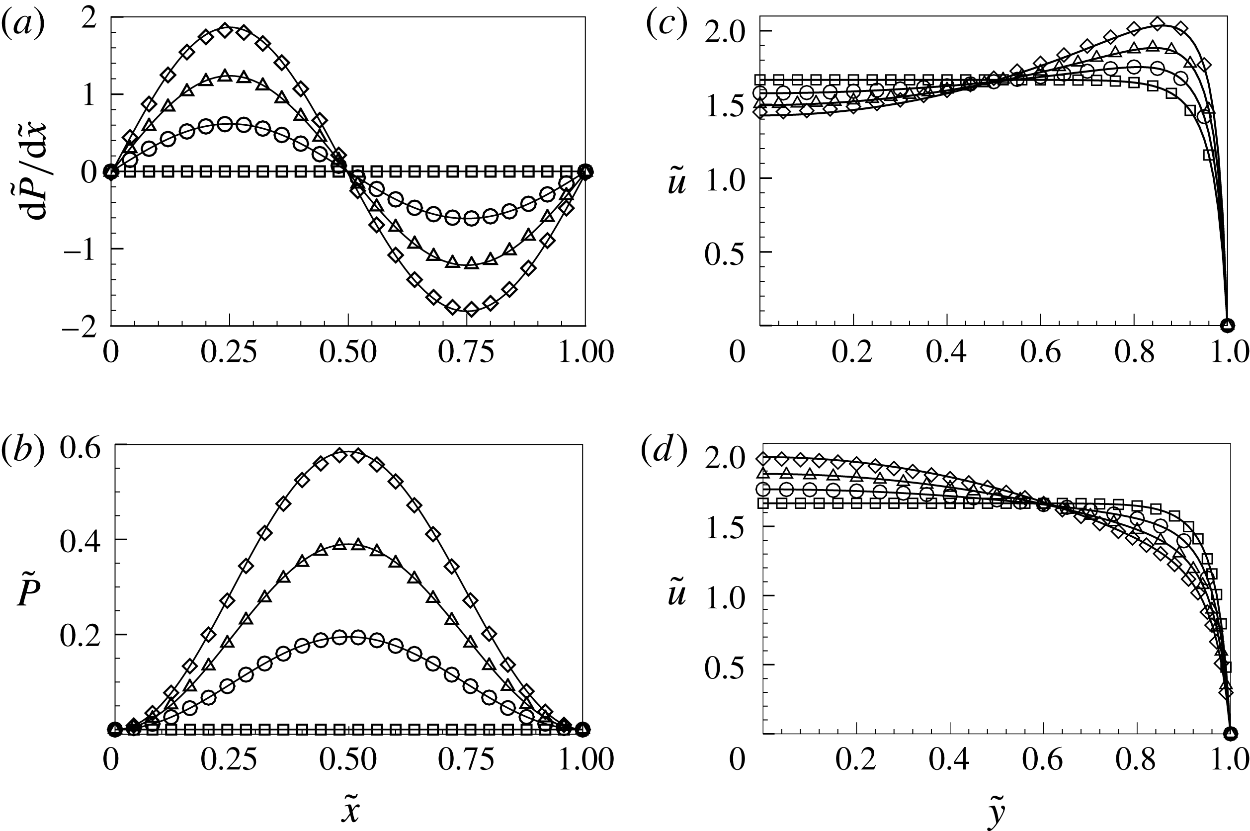
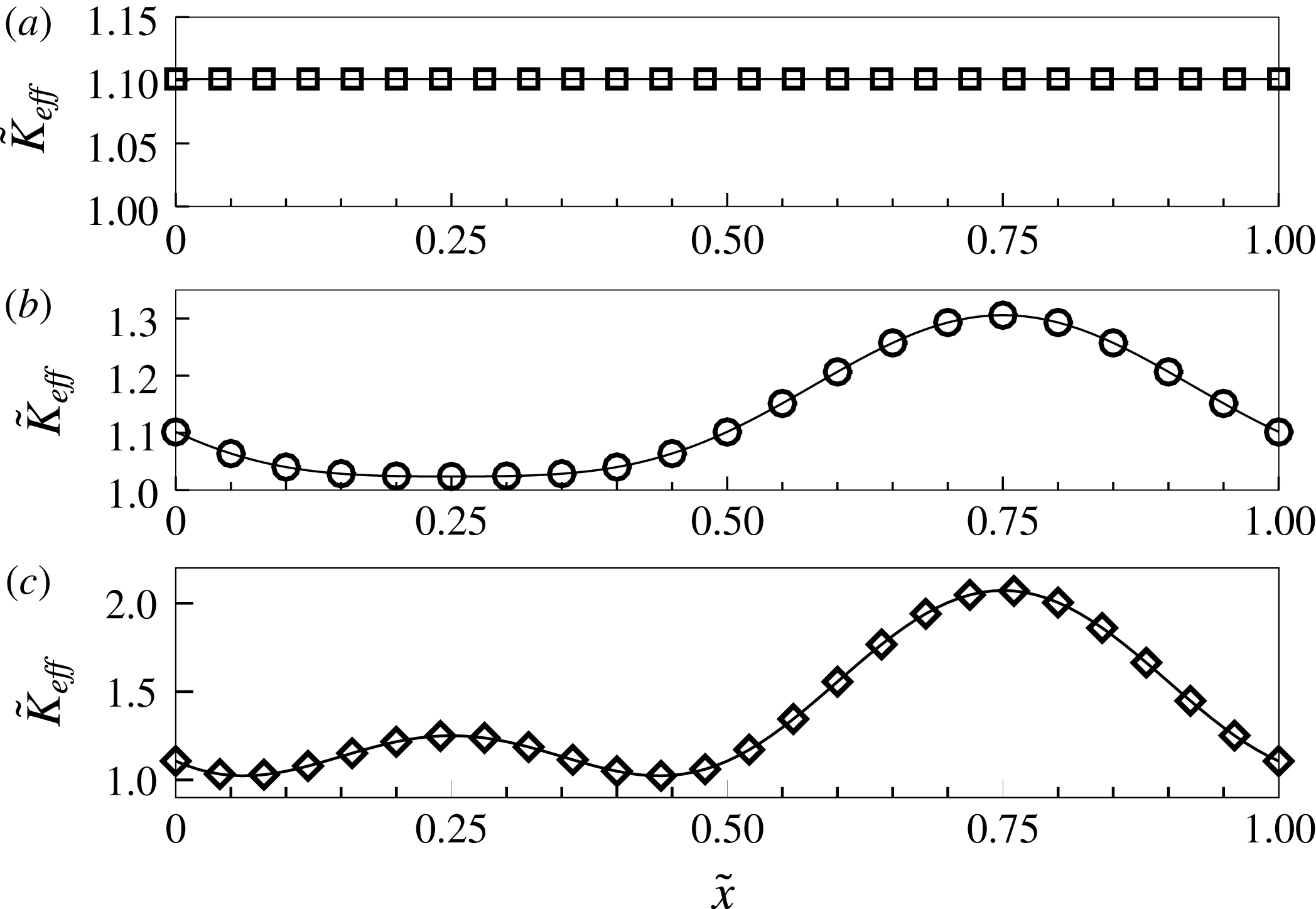
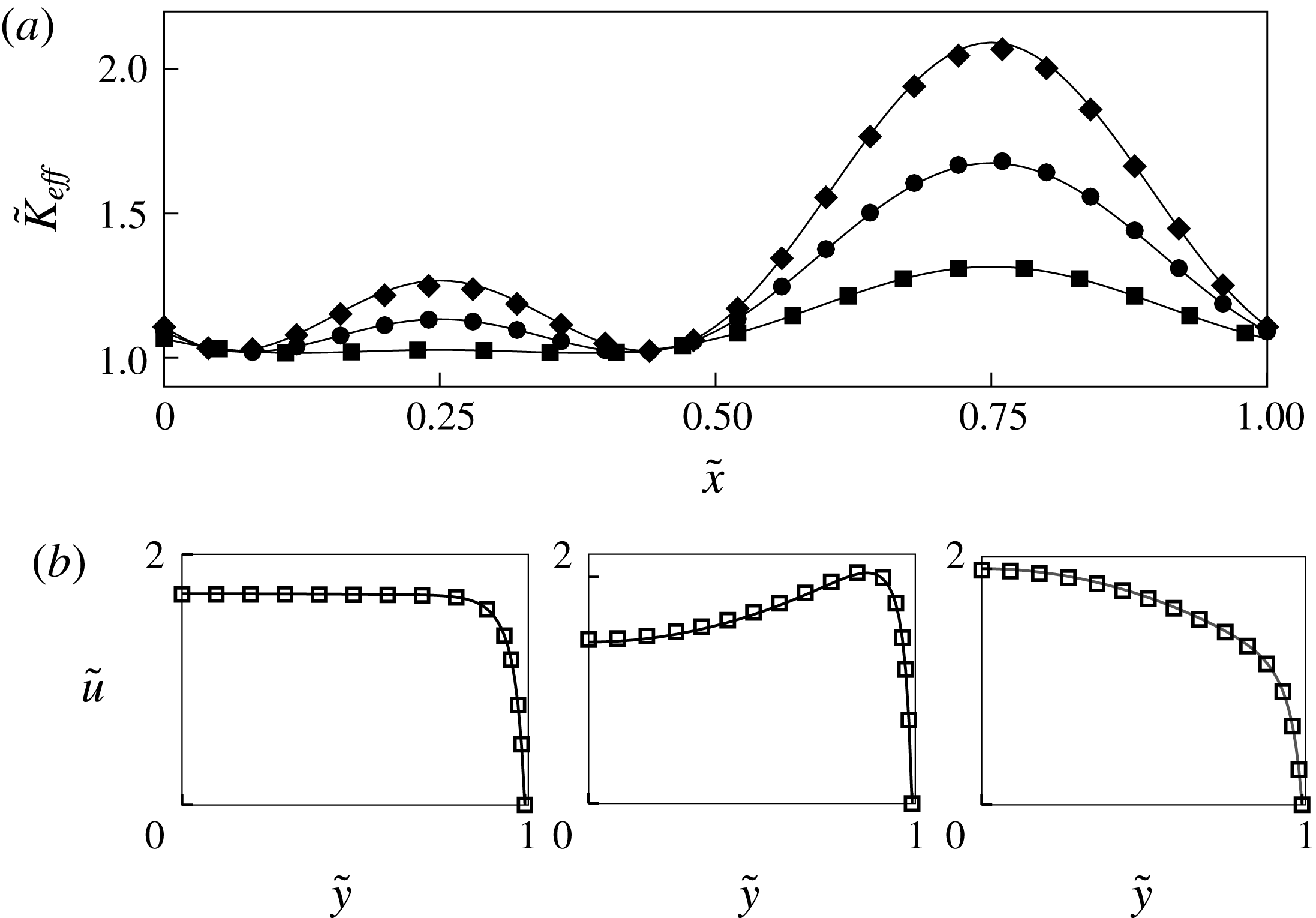
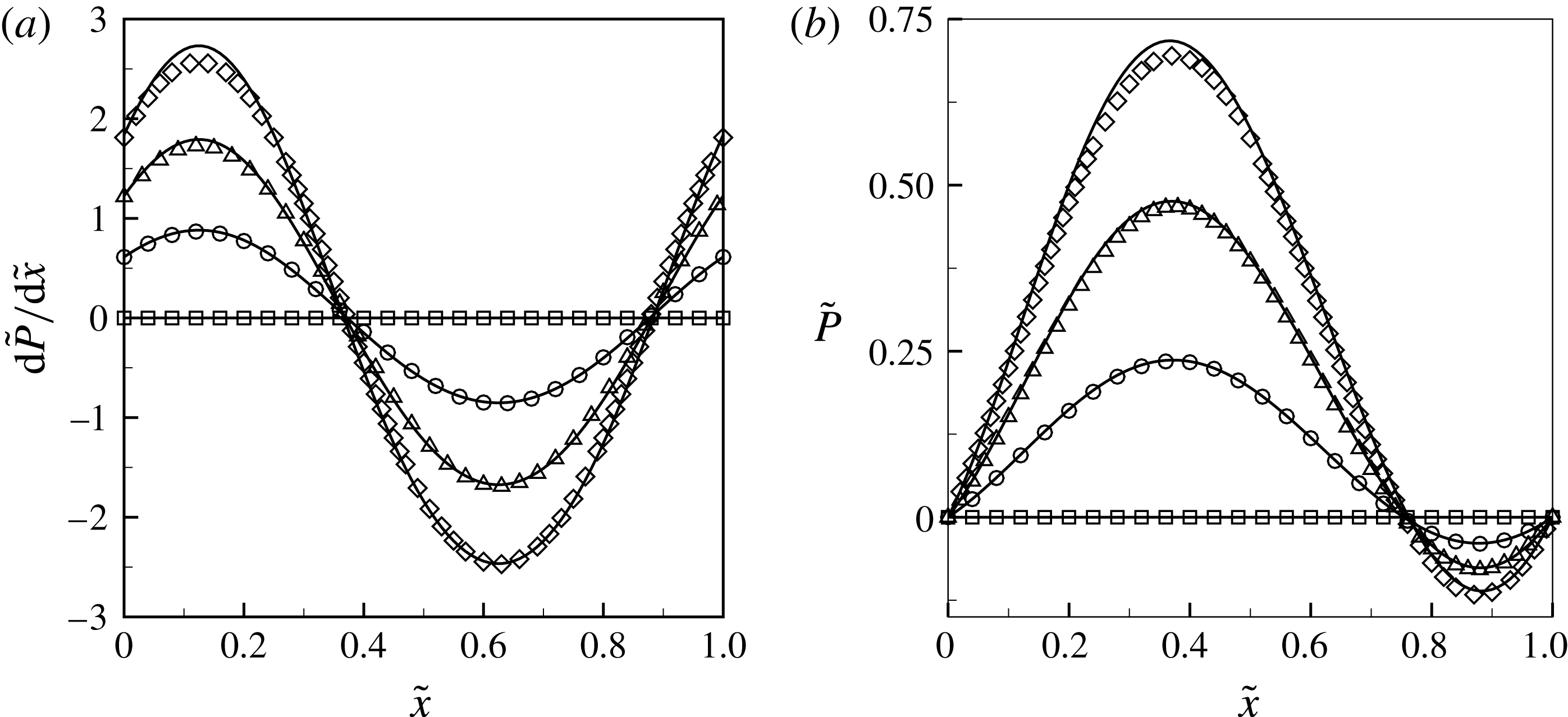
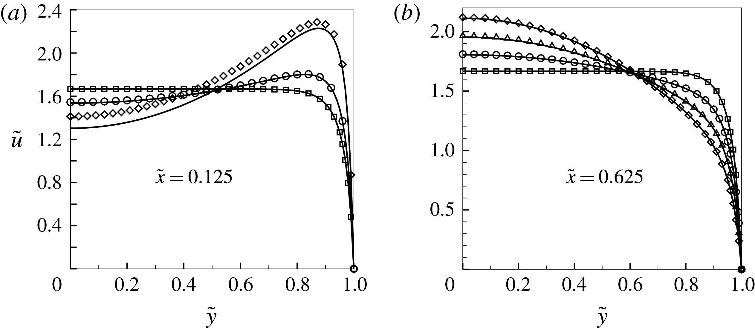
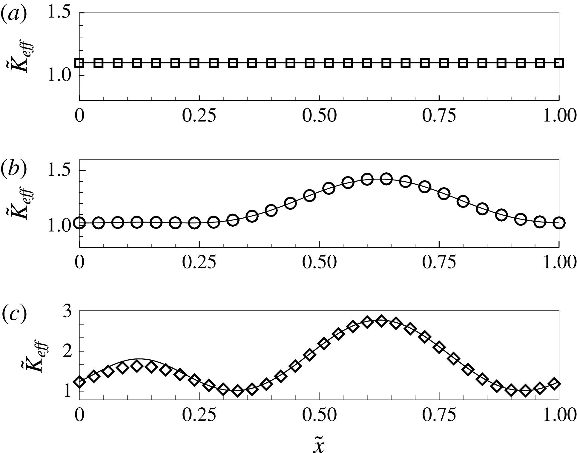
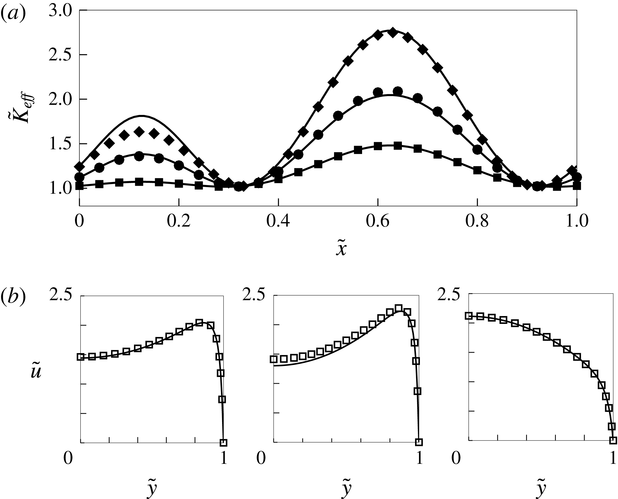
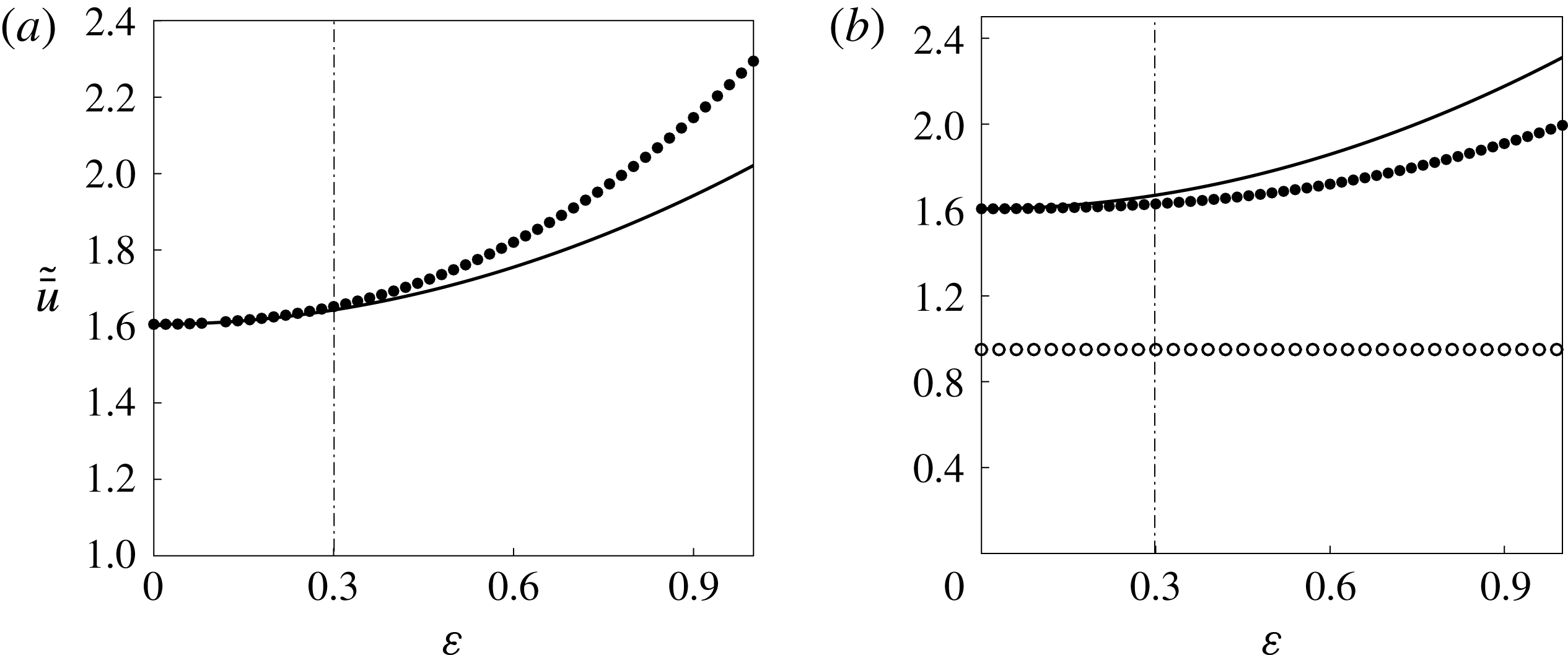
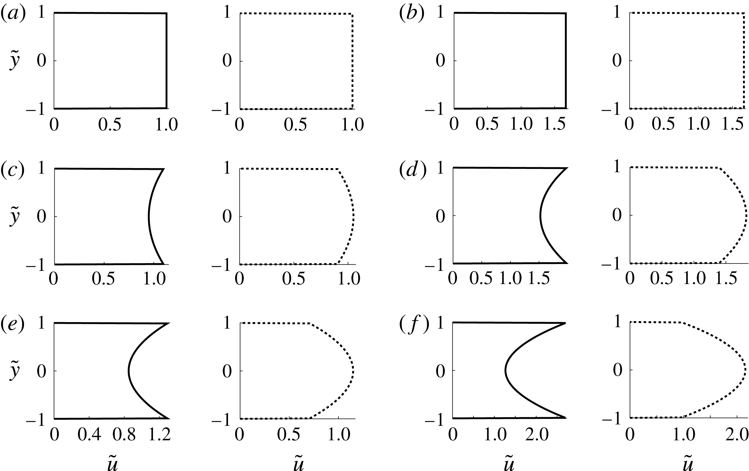
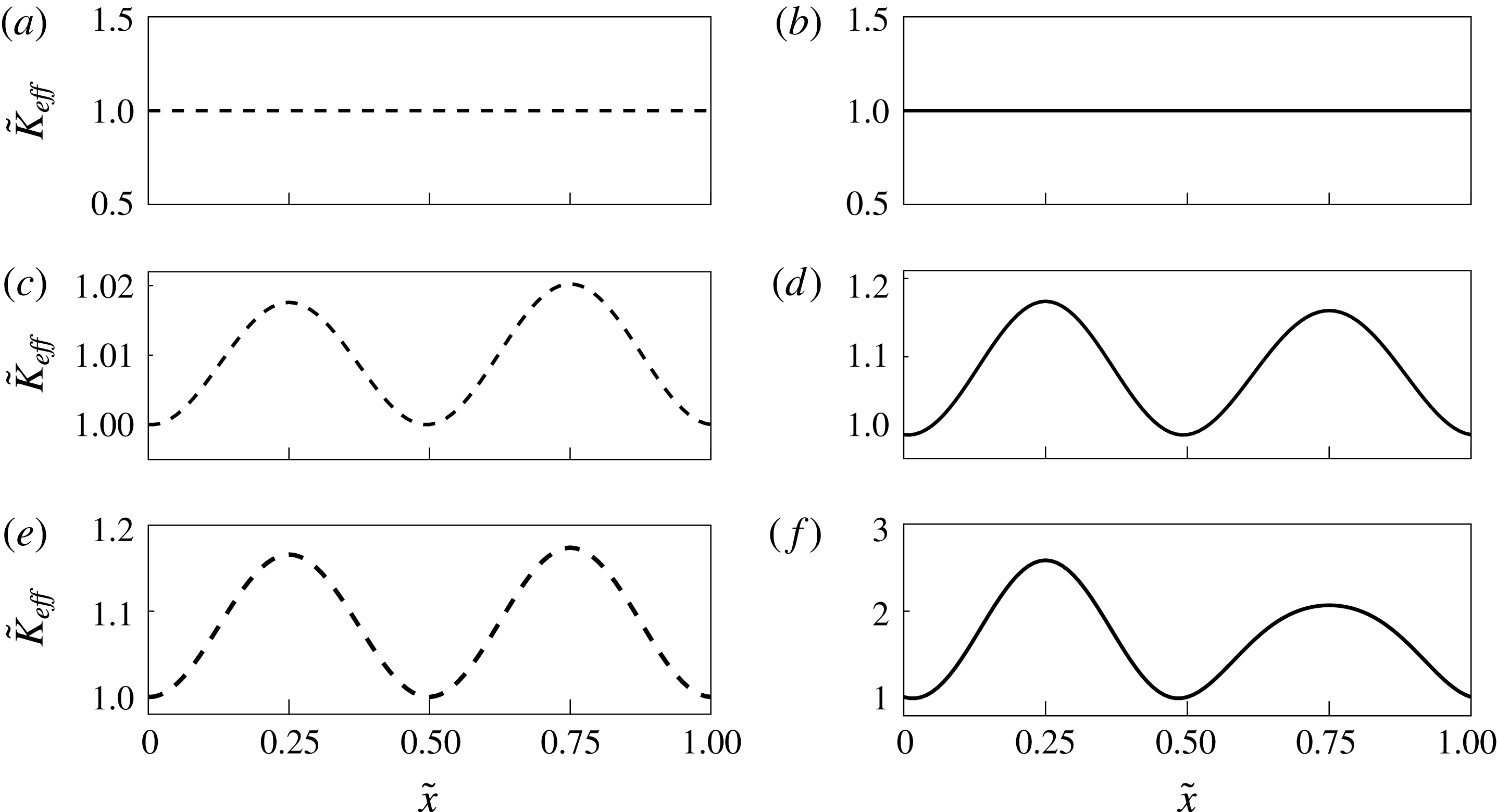
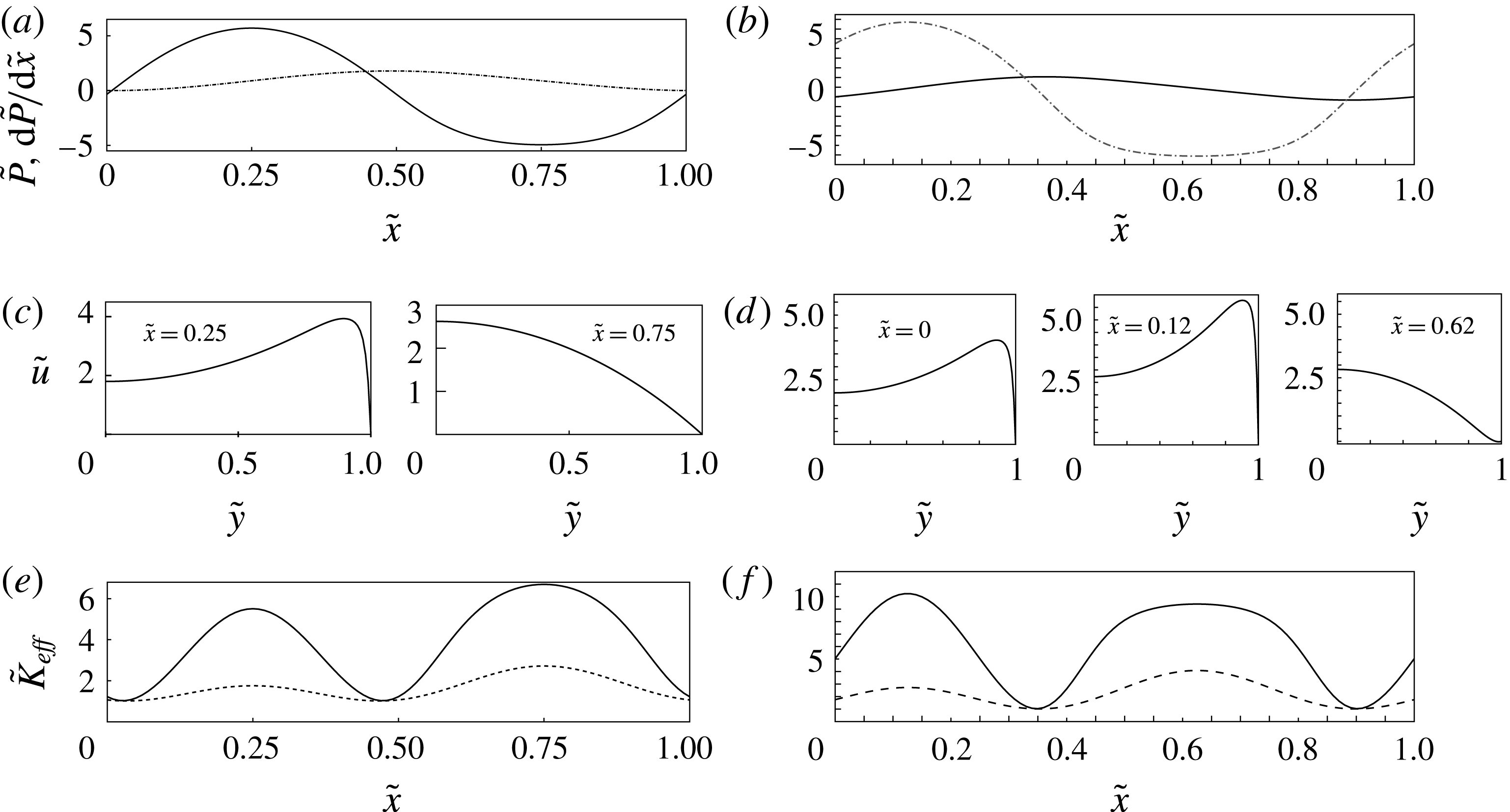
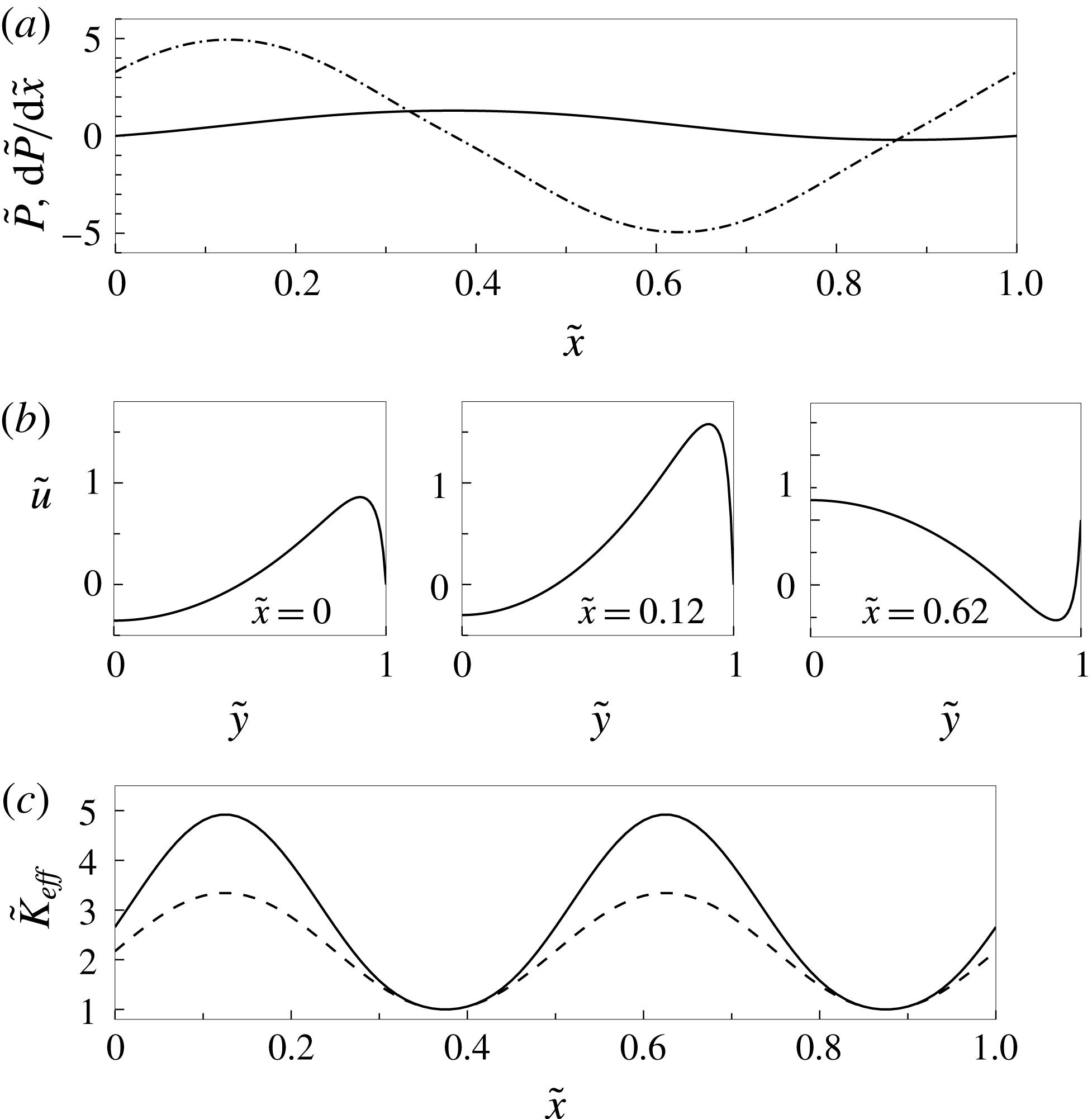
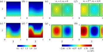
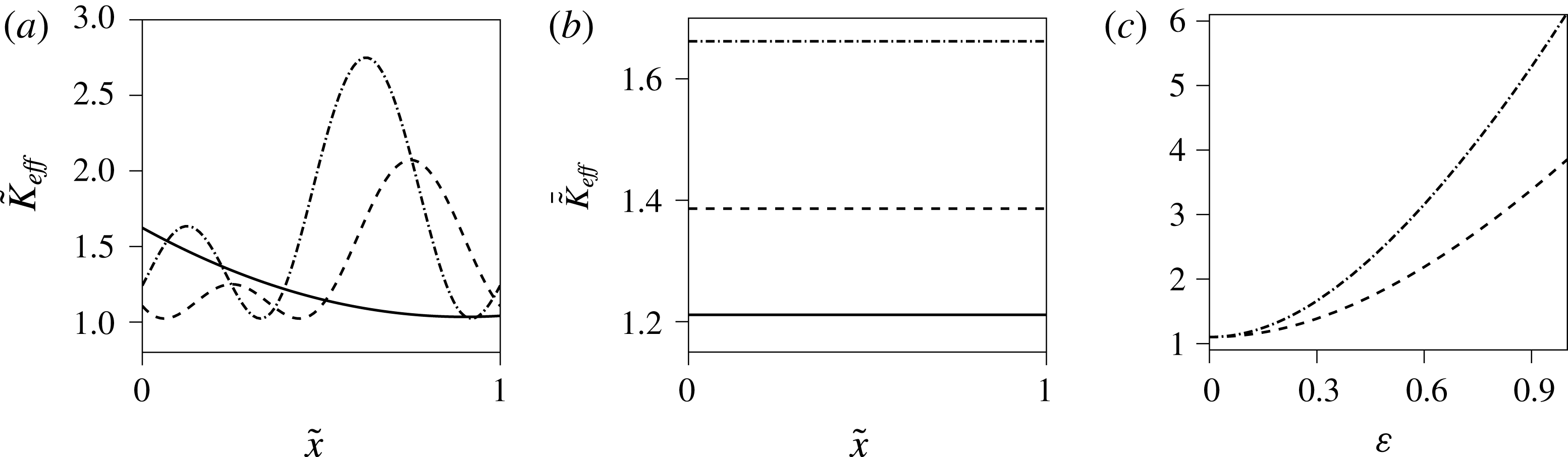
In figures 2–9, the solid lines represent the asymptotic solution determined in § 5, and the symbols refer to the numerical solution. As shown, the hydrodynamic field predicted by the approximate solution is in excellent agreement with the numerical solution when
 $0<\unicode[STIX]{x1D700}\leqslant 0.3$
.
Hydrodynamic behaviour under the influence of
 $\tilde{\unicode[STIX]{x1D701}}=1+\unicode[STIX]{x1D700}\tilde{\unicode[STIX]{x1D701}}_{1}$
with
 $\unicode[STIX]{x1D70E}_{1}=1$
and
 $\unicode[STIX]{x1D70E}_{2}=0$
. Here
 $\tilde{\unicode[STIX]{x1D716}}De^{2}=1$
and
 $\tilde{\unicode[STIX]{x1D705}}=20$
, for (▫)
 $\unicode[STIX]{x1D700}=0$
, (○)
 $\unicode[STIX]{x1D700}=0.1$
, (▵)
 $\unicode[STIX]{x1D700}=0.2$
, and (♢)
 $\unicode[STIX]{x1D700}=0.3$
. (a,b) Dimensionless pressure gradient
 $\text{d}\tilde{P}/\text{d}\tilde{x}$
and the dimensionless pressure
 $\tilde{P}$
plotted as functions of the dimensionless axial direction
 $\tilde{x}$
. (c,d) Dimensionless velocity profiles as functions of the transversal variable
 ${\tilde{y}}$
evaluated at arbitrary values of
 $\tilde{x}=0.25$
and
 $\tilde{x}=0.75$
, respectively.

Axial variation of
 $\tilde{K}_{eff}$
in the electro-osmotic flow caused by a slowly varying wall potential
 $\tilde{\unicode[STIX]{x1D701}}$
with
 $(\unicode[STIX]{x1D70E}_{1},\unicode[STIX]{x1D70E}_{2})=(1,0)$
. Here, we used
 $\tilde{\unicode[STIX]{x1D716}}De^{2}=1$
,
 $Pe=10$
and
 $\tilde{\unicode[STIX]{x1D705}}=20$
. (a)
 $\unicode[STIX]{x1D700}=0$
, (b)
 $\unicode[STIX]{x1D700}=0.1$
and (c)
 $\unicode[STIX]{x1D700}=0.3$
.

(a) Axial variation of
 $\tilde{K}_{eff}$
in the electro-osmotic flow caused by a slowly varying wall potential
 $\tilde{\unicode[STIX]{x1D701}}=1+\unicode[STIX]{x1D700}\tilde{\unicode[STIX]{x1D701}}_{1}$
with
 $(\unicode[STIX]{x1D70E}_{1},\unicode[STIX]{x1D70E}_{2})=(1,0)$
. Here,
 $Pe=10$
,
 $\tilde{\unicode[STIX]{x1D705}}=20$
and
 $\unicode[STIX]{x1D700}=0.3$
. Several values of the parameter
 $\tilde{\unicode[STIX]{x1D716}}De^{2}$
were selected: (▪)
 $\tilde{\unicode[STIX]{x1D716}}De^{2}=0$
, (●)
 $\tilde{\unicode[STIX]{x1D716}}De^{2}=0.5$
, and (♦)
 $\tilde{\unicode[STIX]{x1D716}}De^{2}=1$
. (b) Dimensionless velocity
 $\tilde{u}$
evaluated at different axial coordinates
 $\tilde{x}(=0,0.25,0.75)$
, from left to right, with
 $\tilde{\unicode[STIX]{x1D716}}De^{2}=1$
.

(a) Induced dimensionless pressure gradient and (b) dimensionless pressure as functions of the coordinate
 $\tilde{x}$
due to the non-uniform
 $\tilde{\unicode[STIX]{x1D701}}=1+\unicode[STIX]{x1D700}\tilde{\unicode[STIX]{x1D701}}_{1}$
for
 $(\unicode[STIX]{x1D70E}_{1},\unicode[STIX]{x1D70E}_{2})=(\sqrt{2},\unicode[STIX]{x03C0}/4)$
. Here,
 $\tilde{\unicode[STIX]{x1D716}}De^{2}=1$
,
 $Pe=10$
and
 $\tilde{\unicode[STIX]{x1D705}}=20$
, for (▫)
 $\unicode[STIX]{x1D700}=0$
, (○)
 $\unicode[STIX]{x1D700}=0.1$
, (▵)
 $\unicode[STIX]{x1D700}=0.2$
and (♢)
 $\unicode[STIX]{x1D700}=0.3$
.

(a,b) Dimensionless velocity
 $\tilde{u}$
as a function of the coordinate
 ${\tilde{y}}$
, evaluated at
 $\tilde{x}(=0.125,0.625)$
. Here,
 $(\unicode[STIX]{x1D70E}_{1},\unicode[STIX]{x1D70E}_{2})=(\sqrt{2},\unicode[STIX]{x03C0}/4)$
in the non-uniform
 $\tilde{\unicode[STIX]{x1D701}}=1+\unicode[STIX]{x1D700}\tilde{\unicode[STIX]{x1D701}}_{1}$
. Additionally,
 $\tilde{\unicode[STIX]{x1D716}}De^{2}=1$
and
 $\tilde{\unicode[STIX]{x1D705}}=20$
, for (▫)
 $\unicode[STIX]{x1D700}=0$
, (○)
 $\unicode[STIX]{x1D700}=0.1$
, (▵)
 $\unicode[STIX]{x1D700}=0.2$
and (♢)
 $\unicode[STIX]{x1D700}=0.3$
.

Axial variation of
 $\tilde{K}_{eff}$
in the electro-osmotic flow caused by a slowly varying wall potential
 $\tilde{\unicode[STIX]{x1D701}}=1+\unicode[STIX]{x1D700}\tilde{\unicode[STIX]{x1D701}}_{1}$
with
 $(\unicode[STIX]{x1D70E}_{1},\unicode[STIX]{x1D70E}_{2})=(\sqrt{2},\unicode[STIX]{x03C0}/4)$
. Here,
 $\tilde{\unicode[STIX]{x1D716}}De^{2}=1$
,
 $Pe=10$
and
 $\tilde{\unicode[STIX]{x1D705}}=20$
; (a)
 $\unicode[STIX]{x1D700}=0$
, (b)
 $\unicode[STIX]{x1D700}=0.1$
and (c)
 $\unicode[STIX]{x1D700}=0.3$
.

(a) Axial variation of
 $\tilde{K}_{eff}$
in the electro-osmotic flow caused by a slowly varying wall potential
 $\tilde{\unicode[STIX]{x1D701}}=1+\unicode[STIX]{x1D700}\tilde{\unicode[STIX]{x1D701}}_{1}$
with
 $(\unicode[STIX]{x1D70E}_{1},\unicode[STIX]{x1D70E}_{2})=(\sqrt{2},\unicode[STIX]{x03C0}/4)$
for
 $\unicode[STIX]{x1D700}=0.3$
,
 $Pe=10$
and
 $\tilde{\unicode[STIX]{x1D705}}=20$
. Here, (▪)
 $\tilde{\unicode[STIX]{x1D716}}De^{2}=0$
, (●)
 $\tilde{\unicode[STIX]{x1D716}}De^{2}=0.5$
and (♦)
 $\tilde{\unicode[STIX]{x1D716}}De^{2}=1$
. (b) Dimensionless velocity
 $\tilde{u}$
evaluated at
 $\tilde{x}(=0,0.125,0.625)$
, from left to right, for
 $\tilde{\unicode[STIX]{x1D716}}De^{2}=1$
.

Dimensionless average velocity,
 $\tilde{\bar{u}}$
, as a function of the parameter
 $\unicode[STIX]{x1D700}$
for
 $\tilde{\unicode[STIX]{x1D716}}De^{2}=1$
and
 $\tilde{\unicode[STIX]{x1D705}}=20$
under the effect of a wall potential
 $\tilde{\unicode[STIX]{x1D701}}=1+\unicode[STIX]{x1D700}\tilde{\unicode[STIX]{x1D701}}_{1}$
. The curves represented by (——) correspond to the asymptotic solutions, and symbol (●) indicates the numerical solution. (a)
 $\tilde{\unicode[STIX]{x1D701}}_{1}$
with
 $(\unicode[STIX]{x1D70E}_{1},\unicode[STIX]{x1D70E}_{2})=(1,0)$
. (b)
 $\tilde{\unicode[STIX]{x1D701}}_{1}$
with
 $(\unicode[STIX]{x1D70E}_{1},\unicode[STIX]{x1D70E}_{2})=(\sqrt{2},\unicode[STIX]{x03C0}/4)$
. The solution represented by (○) refers to the well-known solution of a pure electro-osmotic flow for a Newtonian fluid (
 $\tilde{\unicode[STIX]{x1D716}}De^{2}=0$
) and uniform wall
 $\unicode[STIX]{x1D701}$
potential (
 $\unicode[STIX]{x1D700}=0$
). The latter was reported by Masliyah & Bhattacharjee (Reference Masliyah and Bhattacharjee2006).

6.1 Finite EDL
A comparison between the asymptotic and numerical solutions of the hydrodynamic behaviour of the EOF analysed in this work is presented in figure 2. In figure 2, the hydrodynamic field of the EOF assuming uniform wall
 $\unicode[STIX]{x1D701}$
potentials along the microchannel is represented by the curves with (▫)
 $\unicode[STIX]{x1D700}=0$
(see Afonso et al.
Reference Afonso, Alves and Pinho2009; Bautista et al.
Reference Bautista, Sánchez, Arcos and Méndez2013). In this case, there is no induced pressure in the flow, and the velocity profiles at any axial position
 $\tilde{x}$
exhibit a plug-like behaviour. Conversely, the curves represented by (○)
 $\unicode[STIX]{x1D700}=0.1$
, (▵)
 $\unicode[STIX]{x1D700}=0.2$
and (♢)
 $\unicode[STIX]{x1D700}=0.3$
describe the behaviour of a pure EOF due to a slowly sinusoidally varying
 $\unicode[STIX]{x1D701}$
potential with
 $(\unicode[STIX]{x1D70E}_{1},\unicode[STIX]{x1D70E}_{2})=(1,0)$
. The strong influence of
 $\tilde{\unicode[STIX]{x1D701}}_{1}$
on the hydrodynamics of the flow is evident, as shown in figure 2(a). It is observed that, for
 $0\leqslant \tilde{x}\leqslant 0.5$
, an adverse pressure gradient is induced, and this gradient increases with
 $\unicode[STIX]{x1D700}$
. In contrast, a favourable pressure gradient is induced for
 $0.5<\tilde{x}\leqslant 1$
. Moreover, it is evident that the pressure gradient decreases with
 $\unicode[STIX]{x1D700}$
. In fact, at
 $\tilde{x}=0.25$
and
 $\tilde{x}=0.75$
, the function
 $\tilde{\unicode[STIX]{x1D701}}_{1}$
reaches maximum and minimum values in such a manner that, at these positions, the dimensionless induced pressure gradient is given by the following relationship:
 $$\begin{eqnarray}\displaystyle & \displaystyle \left.\frac{\text{d}\tilde{P}}{\text{d}\tilde{x}}\right|_{\tilde{x}=0.25,0.75}\approx \pm \frac{40\unicode[STIX]{x1D700}\left(57+118\tilde{\unicode[STIX]{x1D716}}De^{2}\right)}{800+351\tilde{\unicode[STIX]{x1D716}}De^{2}}+O(\unicode[STIX]{x1D700}^{2}), & \displaystyle\end{eqnarray}$$
which is obtained from (5.1) after the pressure and consequently the pressure gradient are obtained. The positive and negative signs in (6.1) correspond to the regions of adverse and favourable dimensionless induced pressure gradients, respectively. If
 $\tilde{\unicode[STIX]{x1D716}}De^{2}=1$
, then the relationship (6.1) is reduced to
 $\text{d}\tilde{P}/\text{d}\tilde{x}\approx \pm 700\unicode[STIX]{x1D700}/1151$
, obtaining the maximum and minimum values of
 $\text{d}\tilde{P}/\text{d}\tilde{x}$
, as shown in figure 2(a). In figure 2(b), the asymptotic and numerical solutions for the induced pressure
 $\tilde{P}$
as a function of axial variable
 $\tilde{x}$
and for various values of
 $\unicode[STIX]{x1D700}$
are shown. In the region where
 $\tilde{\unicode[STIX]{x1D701}}_{1}>0$
, the pressure increases, whereas it decreases when
 $\tilde{\unicode[STIX]{x1D701}}_{1}<0$
, acquiring the dimensionless pressure as a non-monotonic distribution. The above means that the axial pressure gradient is induced to meet the requirement of mass continuity. In this context, the asymptotic and numerical solutions are plotted in figure 2(c) for comparison. The velocity profiles
 $\tilde{u}$
are plotted at a selected coordinate of
 $\tilde{x}=0.25$
, which corresponds to the region of the adverse pressure gradient. As shown,
 $\tilde{u}$
is distorted, exhibiting a concave profile over the cross-section of the microchannel. When the wall
 $\unicode[STIX]{x1D701}$
potential is modulated and the parameter
 $\unicode[STIX]{x1D700}$
takes values from 0.1 to 0.3, the concave effect is more pronounced, and the flow appears to have a retarding effect at the centre of the microchannel. In this way, by considering the terms
 $\tilde{u} _{0}$
and
 $\tilde{u} _{1}$
from (5.1) evaluated at
 ${\tilde{y}}=0$
and using (6.1), we can estimate the dimensionless maximum velocity
 $\tilde{u} =\tilde{u} |_{max}$
, which is given by
 $$\begin{eqnarray}\displaystyle \left.\tilde{u} \right|_{max} & {\approx} & \displaystyle 1+\frac{2}{3}\tilde{\unicode[STIX]{x1D716}}De^{2}\pm \unicode[STIX]{x1D700}\left\{1-\frac{20\left(57+118\tilde{\unicode[STIX]{x1D716}}De^{2}\right)}{800+351\tilde{\unicode[STIX]{x1D716}}De^{2}}\right.\nonumber\\ \displaystyle & & \displaystyle \left.+\,\tilde{\unicode[STIX]{x1D716}}De^{2}\left[2-\frac{117}{20}\frac{\left(57+118\tilde{\unicode[STIX]{x1D716}}De^{2}\right)}{800+351\tilde{\unicode[STIX]{x1D716}}De^{2}}\right]\right\}+O(\unicode[STIX]{x1D700}^{2}).\end{eqnarray}$$
The signs
 $+$
and
 $-$
in the third term on the right-hand side of (6.2) correspond to the regions of adverse and favourable dimensionless pressure gradients, respectively. In (6.2), if
 $\unicode[STIX]{x1D700}=0$
, then
 $\left.\tilde{u} \right|_{max}\approx 1+\frac{2}{3}\tilde{\unicode[STIX]{x1D716}}De^{2}$
(see Afonso et al.
Reference Afonso, Alves and Pinho2009; Bautista et al.
Reference Bautista, Sánchez, Arcos and Méndez2013). For the adverse dimensionless pressure gradient and
 $\tilde{\unicode[STIX]{x1D716}}De^{2}=1$
, the relationship (6.2) is reduced to
 $\left.\tilde{u} \right|_{max}\approx (5/3)-(4283/4604)\unicode[STIX]{x1D700}+O(\unicode[STIX]{x1D700}^{2})$
at
 $\tilde{x}=0.25$
, and it provides the value of the velocity at the centre of the microchannel, being smaller than that near the wall, as shown in figure 2(c); therefore, the velocity profiles are distorted with a concave shape in the flow direction. Meanwhile, in the region of the favourable pressure gradient, the dimensionless velocity profiles
 $\tilde{u}$
as a function of the transversal variable
 ${\tilde{y}}$
evaluated at
 $\tilde{x}=0.75$
and for various values of
 $\unicode[STIX]{x1D700}$
are as plotted in figure 2(d). For
 $\tilde{\unicode[STIX]{x1D716}}De^{2}=1$
, the relationship (6.2) is reduced to
 $\left.\tilde{u} \right|_{max}\approx (5/3)+(4283/4604)\unicode[STIX]{x1D700}+O(\unicode[STIX]{x1D700}^{2})$
and reproduces the values of the dimensionless velocities at the centre being larger than that near the wall; then, the profiles of
 $\tilde{u}$
are distorted, exhibiting a slightly convex behaviour. When varying the parameter
 $\unicode[STIX]{x1D700}$
from 0.1 to 0.3 in the
 $\tilde{\unicode[STIX]{x1D701}}$
potential, the convex effect on the velocity profiles is increasingly more pronounced through the microchannel.
6.2 Dispersion coefficient,
$\tilde{K}_{eff}$

Figure 3 shows the axial variation of the dimensionless effective dispersion coefficient
 $\tilde{K}_{eff}$
of the EOF for an sPTT fluid model under the influence of a varying
 $\unicode[STIX]{x1D701}$
potential. In this figure, solid lines indicate the asymptotic solution given in (5.16), and symbols are the numerical solution given by (4.1) and (4.3). If we assume the condition of a uniform wall potential, i.e.
 $\tilde{\unicode[STIX]{x1D701}}=1$
, the curve given in panel (a) for
 $\unicode[STIX]{x1D700}=0$
represents the pure diffusional dispersion behaviour for an sPTT fluid model with uniform velocity profiles (see figure 2). In this limit, one recovers from (5.16) that
 $\tilde{K}_{eff}\approx 1.1009$
, i.e. the diffusional dispersion is increased approximately 10
 $\%$
, with
 $\tilde{\unicode[STIX]{x1D716}}De^{2}=1$
, in comparison with the case of a Newtonian fluid. When the wall
 $\unicode[STIX]{x1D701}$
potential is slowly modulated by means of the dimensionless amplitude
 $\unicode[STIX]{x1D700}(=0.1,0.3)$
, the flow has a non-uniform behaviour along the microchannel, causing adverse and favourable pressure gradients; consequently, the concave and convex shapes of the velocity profiles strongly distort the distribution of
 $\tilde{K}_{eff}$
along the microchannel, significantly contributing to the diffusional dispersion coefficient, as shown in figure 3. The pure diffusional dispersion is always recovered at the axial coordinates
 $\tilde{x}(=0,0.5,1)$
for any value of the parameter
 $\unicode[STIX]{x1D700}$
. In figure 3(b), for
 $\unicode[STIX]{x1D700}=0.1$
, we observe that due to a retarding effect in the electrokinetic flow at the region
 $0\leqslant \tilde{x}\leqslant 0.5$
, the local value of
 $\tilde{K}_{eff}$
decreases below that obtained when
 $\unicode[STIX]{x1D700}=0$
(panel a); by contrast, for
 $0.5\leqslant \tilde{x}\leqslant 1$
, an accelerated effect on the flow tends to increase the local value of the effective dispersion coefficient
 $\tilde{K}_{eff}$
, whose value is greater than that of pure diffusional dispersion of an sPTT fluid model. When the amplitude
 $\unicode[STIX]{x1D700}$
is increased, the maximum value of the adverse dimensionless pressure gradient is found at
 $\tilde{x}=0.25$
, which has an important influence on
 $\tilde{K}_{eff}$
, mostly in the vicinity of the aforementioned coordinate. This is a consequence arising from the velocity gradients because they become stronger due to the non-uniformity in the velocity flow, generating higher values in dispersion in comparison with pure diffusional dispersion, as shown for
 $\unicode[STIX]{x1D700}=0.3$
in figure 3(c). In contrast, for
 $0.5\leqslant \tilde{x}\leqslant 1$
, the electrokinetic flow has a convex velocity profile, which may produce significant variations in
 $\tilde{K}_{eff}$
precisely because the velocity gradient is sufficiently high due to the appearance of favourable induced pressure gradients, with a strong influence near the position
 $\tilde{x}=0.75$
.
To highlight the enhancement in dispersion due to viscoelastic effects, the effective dispersion coefficient is plotted as a function of the axial position for three values of the viscoelastic parameter
 $\tilde{\unicode[STIX]{x1D716}}De^{2}$
in figure 4(a). The curve using ▪ denotes
 $\tilde{\unicode[STIX]{x1D716}}De^{2}=0$
, corresponding to the Newtonian fluid. The curves with ● and ♦ correspond to
 $\tilde{\unicode[STIX]{x1D716}}De^{2}=0.5$
and
 $\tilde{\unicode[STIX]{x1D716}}De^{2}=1$
, respectively. As shown, the viscoelastic parameter significantly enhances the axial dimensionless effective dispersion because the velocity gradients increase with
 $\tilde{\unicode[STIX]{x1D716}}De^{2}$
due to increasing levels of shear thinning, both within the EDL layer and in the bulk zone (Afonso et al.
Reference Afonso, Alves and Pinho2009); this means that
 $\tilde{\unicode[STIX]{x1D716}}De^{2}$
has a stronger influence in the region
 $0.5\leqslant \tilde{x}\leqslant 1$
(favourable pressure gradient) than in the region of
 $0\leqslant \tilde{x}\leqslant 0.5$
(adverse pressure gradient region). Figure 4(b) shows velocity profiles evaluated at three different coordinates
 $\tilde{x}(=0,0.25,0.75)$
when a varying wall
 $\tilde{\unicode[STIX]{x1D701}}$
potential is imposed. Note that flat shapes in the velocity profiles are present at positions
 $\tilde{x}(=0,0.5,1)$
, and on the region of the adverse pressure gradient, a concave shape of the velocity is developed at
 $\tilde{x}=0.25$
. In the region of the favourable pressure gradient, the velocity has a convex shape at
 $\tilde{x}=0.75$
. As expected, the effect of a convex shape of the velocity profile contributes more effectively to the dispersion coefficients compared to that of the concave profile, as was discussed by Ng & Zhou (Reference Ng and Zhou2012a
).
The electrokinetic hydrodynamics under the influence of the slowly varying wall
 $\tilde{\unicode[STIX]{x1D701}}$
potential with
 $(\unicode[STIX]{x1D70E}_{1},\unicode[STIX]{x1D70E}_{2})=(\sqrt{2},\unicode[STIX]{x03C0}/4)$
is presented in figures 5 and 6. In this context, the axial distribution of the effective dispersion coefficient is plotted in figures 7 and 8. As shown, the pressure gradient must then have the same dependence on
 $\tilde{x}$
according to
 $\tilde{\unicode[STIX]{x1D701}}_{1}$
. In this case, two adverse pressure gradient regions appear: one of them for (
 $0\leqslant \tilde{x}\leqslant 0.375$
) and the other for (
 $0.875\leqslant \tilde{x}\leqslant 1$
). Additionally, a favourable pressure gradient region is located for (
 $0.375<\tilde{x}<0.875$
), as depicted in figure 5(a). The dimensionless pressure gradient has maximum and minimum values at
 $\tilde{x}(=0.125,0.625)$
, respectively, where the axial pressure distribution takes negative values in the region
 $0.75<\tilde{x}<1$
because it is needed to satisfy the boundary condition of pressure at the exit of the microchannel, as shown in figure 5(b). When the wall
 $\tilde{\unicode[STIX]{x1D701}}$
potential is modulated by increasing the amplitude
 $\unicode[STIX]{x1D700}$
from 0.1 to 0.3, the concave and convex shapes of the velocity profiles generated by adverse–favourable pressure gradients are greater than those obtained with
 $(\unicode[STIX]{x1D70E}_{1},\unicode[STIX]{x1D70E}_{2})=(1,0)$
for the same numerical values of
 $\tilde{\unicode[STIX]{x1D716}}De^{2}$
,
 $\tilde{\unicode[STIX]{x1D705}}$
and
 $\unicode[STIX]{x1D700}$
, as can be confirmed in figure 2.
Figure 7 presents the axial distribution of the dispersion coefficient
 $\tilde{K}_{eff}$
generated due to the aforementioned hydrodynamic behaviour shown in figures 5 and 6, where the maximum and minimum values of the wall
 $\tilde{\unicode[STIX]{x1D701}}$
potential are found at the coordinates
 $\tilde{x}(=0.125,0.625)$
, respectively. In this case, the local effective dispersion coefficient
 $\tilde{K}_{eff}$
is higher than the value obtained with the non-uniform flow generated by the
 $\tilde{\unicode[STIX]{x1D701}}$
potential with
 $(\unicode[STIX]{x1D70E}_{1},\unicode[STIX]{x1D70E}_{2})=(1,0)$
, in which the maximum and minimum values of
 $\tilde{\unicode[STIX]{x1D701}}$
were located at
 $\tilde{x}=0.25$
and
 $\tilde{x}=0.75$
, respectively. In general, with the combined effects of viscoelasticity
 $\tilde{\unicode[STIX]{x1D716}}De^{2}$
and when the modulation
 $\unicode[STIX]{x1D700}$
is increased from 0.1 to 0.3, the axial dispersion coefficient
 $\tilde{K}_{eff}$
is greater than that of the pure molecular diffusion (
 $\unicode[STIX]{x1D700}=0$
), shown in figure 7(a).
In figure 8(a), the axial variation of the dispersion coefficient
 $\tilde{K}_{eff}$
with a slowly varying wall
 $\tilde{\unicode[STIX]{x1D701}}$
potential with
 $(\unicode[STIX]{x1D70E}_{1},\unicode[STIX]{x1D70E}_{2})=(\sqrt{2},\unicode[STIX]{x03C0}/4)$
under the influence of the viscoelastic parameter
 $\tilde{\unicode[STIX]{x1D716}}De^{2}$
is plotted. As shown, the axial dispersion coefficient for the Newtonian case (▪) is always smaller than that of viscoelastic fluids. Moreover, the dispersion coefficient varies in a non-monotonic manner in the
 $\tilde{x}$
direction. In addition, greater values of
 $\tilde{K}_{eff}$
are achieved as the viscoelastic parameter is increased. At the coordinates
 $\tilde{x}(=0.125,0.625)$
, the local dispersion coefficient is notably increased provided that
 $\text{d}\tilde{P}/\text{d}\tilde{x}$
reaches its maximum and minimum values at these positions. Additionally, due to the form of
 $\tilde{\unicode[STIX]{x1D701}}_{1}$
, and in accordance with the appearance of two regions of adverse pressure gradients, as depicted in 5(a), concave shapes of the velocity profiles at
 $\tilde{x}(=0,0.125)$
are found and, at the latter position, the local maximum dispersion coefficient
 $\tilde{K}_{eff}$
is obtained. Conversely, in the region of the favourable pressure gradient (
 $\tilde{x}=0.625$
), the velocity profile is convex; consequently,
 $\tilde{K}_{eff}$
provides its global maximum value. Higher values in
 $\tilde{K}_{eff}$
are achieved when
 $(\unicode[STIX]{x1D70E}_{1},\unicode[STIX]{x1D70E}_{2})=(\sqrt{2},\unicode[STIX]{x03C0}/4)$
in comparison with that obtained with
 $(\unicode[STIX]{x1D70E}_{1},\unicode[STIX]{x1D70E}_{2})=(1,0)$
. When the viscoelastic parameter
 $\tilde{\unicode[STIX]{x1D716}}De^{2}$
is increased, as shown in figures 4(a) and 8(a), the aforementioned behaviour is primarily because plug-like velocity profiles are developed
 $(\unicode[STIX]{x1D70E}_{1},\unicode[STIX]{x1D70E}_{2})=(1,0)$
near the entrance and exit of the microchannel. In contrast, lower values are achieved when
 $(\unicode[STIX]{x1D70E}_{1},\unicode[STIX]{x1D70E}_{2})=(\sqrt{2},\unicode[STIX]{x03C0}/4)$
and convex profiles are present in these regions.
Figure 9 shows the dimensionless average velocity
 $\tilde{\bar{u}}$
as a function of the dimensionless amplitude of the fluctuations
 $\unicode[STIX]{x1D700}$
under the influence of the varying wall potential
 $\tilde{\unicode[STIX]{x1D701}}_{1}$
. For the asymptotic solution, when
 $\unicode[STIX]{x1D700}=0$
, the leading order
 $\tilde{\bar{u}}_{0}$
represents the well-known dimensionless average velocity for the pure EOF of a viscoelastic fluid with a constant wall
 $\tilde{\unicode[STIX]{x1D701}}$
potential reported previously (Afonso et al.
Reference Afonso, Alves and Pinho2009; Bautista et al.
Reference Bautista, Sánchez, Arcos and Méndez2013). In this case, the dimensionless average velocity reaches the value of
 $\tilde{\bar{u}}=1.6$
. The terms
 $O(\unicode[STIX]{x1D700}^{1})$
and
 $(\unicode[STIX]{x1D700}^{2})$
are corrections to the leading order (5.3), which take the contributions of the combined effects of
 $\tilde{\unicode[STIX]{x1D701}}_{1}$
and the viscoelastic parameter
 $\tilde{\unicode[STIX]{x1D716}}De^{2}$
on the dimensionless average velocity
 $\tilde{\bar{u}}$
into account, as shown in figure 9. For increasing values of
 $\unicode[STIX]{x1D700}>0$
, the dimensionless average velocity increases, irrespective of the form that the wall
 $\unicode[STIX]{x1D701}$
potential assumes. The dimensionless average velocity for the EOF of a Newtonian fluid with a uniform wall
 $\tilde{\unicode[STIX]{x1D701}}$
potential obtains a value of
 $\tilde{\bar{u}}\approx 0.95$
and is represented in figure 9(b) by ○. When
 $\unicode[STIX]{x1D700}\approx$
0.3, the dimensionless average velocity has a value of
 $\tilde{\bar{u}}\approx$
1.675, representing an increase of approximately 76
 $\%$
with respect to the Newtonian case. Additionally, figure 9 confirms the efficacy of the approximate solution, which can be judged by comparing the approximate (——) and numerical (●) solutions, revealing excellent agreement up to values of
 $\unicode[STIX]{x1D700}\approx 0.3$
. The above is because the solutions for each dependent variable defined in (5.1) are restricted to small values of
 $\unicode[STIX]{x1D700}$
. As was expected, in the limit of
 $\unicode[STIX]{x1D700}\rightarrow 0$
, the solution of the problem with a uniform
 $\unicode[STIX]{x1D701}$
potential was obtained, and, for small
 $\unicode[STIX]{x1D700}$
, any variable
 $X=\tilde{u}$
,
 $\tilde{v}$
,
 $\tilde{\bar{u}}$
and
 $\tilde{P}$
together with
 $\tilde{K}_{eff}$
depart from their limiting (uniform
 $\tilde{\unicode[STIX]{x1D701}}$
-potential) behaviour in a way that depends smoothly on
 $\unicode[STIX]{x1D700}$
. This is the nature of breakdown of the asymptotic approximation with the numerical results, as clearly shown in figure 9.
6.3 Thin EDL:
$\tilde{\unicode[STIX]{x1D705}}\gg 1$

We are also interested in highlighting the hydrodynamic dispersion for an EOF for the case of large
 $\tilde{\unicode[STIX]{x1D705}}$
(i.e. in the thin EDL limit). In this limit, the terms
 $\tilde{u} _{0}$
,
 $\tilde{u} _{1}$
and
 $\tilde{u} _{2}$
of the asymptotic solution for the velocity represented in (5.2), (5.4) and (5.10) are simplified and shown in appendix C through equations (C 1)–(C 3). Furthermore, the terms defined in the supplementary material by
 $\unicode[STIX]{x1D6F1}_{i}$
(
 $i=1,\ldots ,25$
) are reduced to
 $\unicode[STIX]{x1D6F1}_{1}=-4/15$
,
 $\unicode[STIX]{x1D6F1}_{2}=1/3$
,
 $\unicode[STIX]{x1D6F1}_{3}=\unicode[STIX]{x1D6F1}_{4}=0$
,
 $\unicode[STIX]{x1D6F1}_{5}=2/5\tilde{\unicode[STIX]{x1D705}}$
,
 $\unicode[STIX]{x1D6F1}_{6}=-4/45$
,
 $\unicode[STIX]{x1D6F1}_{7}=\unicode[STIX]{x1D6F1}_{8}=0$
,
 $\unicode[STIX]{x1D6F1}_{9}=-1/\tilde{\unicode[STIX]{x1D705}}$
,
 $\unicode[STIX]{x1D6F1}_{10}=2/9$
,
 $\unicode[STIX]{x1D6F1}_{i}=0(i=11,\ldots ,18)$
,
 $\unicode[STIX]{x1D6F1}_{19}=-4/3\tilde{\unicode[STIX]{x1D705}}$
,
 $\unicode[STIX]{x1D6F1}_{20}=4/27$
,
 $\unicode[STIX]{x1D6F1}_{21}=1/3$
,
 $\unicode[STIX]{x1D6F1}_{22}=\unicode[STIX]{x1D6F1}_{23}=0$
,
 $\unicode[STIX]{x1D6F1}_{24}=-1/\tilde{\unicode[STIX]{x1D705}}$
, and
 $\unicode[STIX]{x1D6F1}_{25}=2/9$
; hence, the effective dispersion coefficient given in (5.16) becomes
 $$\begin{eqnarray}\displaystyle \tilde{K}_{eff} & = & \displaystyle 1+Pe^{2}\left\{\frac{17}{315}\left(\frac{\text{d}\tilde{P}}{\text{d}\tilde{x}}\right)^{2}-\frac{4}{15}\tilde{\unicode[STIX]{x1D701}}\frac{\text{d}\tilde{P}}{\text{d}\tilde{x}}+\frac{1}{3}\tilde{\unicode[STIX]{x1D701}}^{2}+2\tilde{\unicode[STIX]{x1D716}}De^{2}\left[\frac{2}{5\tilde{\unicode[STIX]{x1D705}}}\tilde{\unicode[STIX]{x1D701}}^{2}\left(\frac{\text{d}\tilde{P}}{\text{d}\tilde{x}}\right)^{2}\right.\right.\nonumber\\ \displaystyle & & \displaystyle \left.\left.-\,\frac{4}{45}\tilde{\unicode[STIX]{x1D701}}^{3}\frac{\text{d}\tilde{P}}{\text{d}\tilde{x}}-\frac{1}{\tilde{\unicode[STIX]{x1D705}}}\tilde{\unicode[STIX]{x1D701}}^{3}\frac{\text{d}\tilde{P}}{\text{d}\tilde{x}}+\frac{2}{9}\tilde{\unicode[STIX]{x1D701}}^{4}\right]+(\tilde{\unicode[STIX]{x1D716}}De^{2})^{2}\left[-\frac{4}{3\tilde{\unicode[STIX]{x1D705}}}\tilde{\unicode[STIX]{x1D701}}^{5}\frac{\text{d}\tilde{P}}{\text{d}\tilde{x}}+\frac{4}{27}\tilde{\unicode[STIX]{x1D701}}^{6}\right]\right\}\nonumber\\ \displaystyle & & \displaystyle -\,2Pe^{2}\tilde{\bar{u}}\left\{-\frac{2}{15}\frac{\text{d}\tilde{P}}{\text{d}\tilde{x}}+\frac{1}{3}\tilde{\unicode[STIX]{x1D701}}+\tilde{\unicode[STIX]{x1D716}}De^{2}\left[-\frac{1}{\tilde{\unicode[STIX]{x1D705}}}\tilde{\unicode[STIX]{x1D701}}^{2}\frac{\text{d}\tilde{P}}{\text{d}\tilde{x}}+\frac{2}{9}\tilde{\unicode[STIX]{x1D701}}^{3}\right]\right\}+\frac{Pe^{2}\tilde{\bar{u}}^{2}}{3}.\end{eqnarray}$$
In this limit, for a viscoelastic fluid, the corresponding function
 $f(\tilde{\unicode[STIX]{x1D705}})$
from (5.18) takes the following form:
 $$\begin{eqnarray}\displaystyle f(\tilde{\unicode[STIX]{x1D705}},\tilde{\unicode[STIX]{x1D716}}De^{2},\unicode[STIX]{x1D700}) & = & \displaystyle \frac{12\tilde{\unicode[STIX]{x1D705}}^{2}}{\tilde{\bar{u}}^{2}}\left\{\frac{17}{315}\left(\frac{\text{d}\tilde{P}}{\text{d}\tilde{x}}\right)^{2}-\frac{4}{15}\tilde{\unicode[STIX]{x1D701}}\frac{\text{d}\tilde{P}}{\text{d}\tilde{x}}+\frac{1}{3}\tilde{\unicode[STIX]{x1D701}}^{2}+2\tilde{\unicode[STIX]{x1D716}}De^{2}\left[\frac{2}{5\tilde{\unicode[STIX]{x1D705}}}\tilde{\unicode[STIX]{x1D701}}^{2}\left(\frac{\text{d}\tilde{P}}{\text{d}\tilde{x}}\right)^{2}\right.\right.\nonumber\\ \displaystyle & & \displaystyle \left.\left.-\,\frac{4}{45}\tilde{\unicode[STIX]{x1D701}}^{3}\frac{\text{d}\tilde{P}}{\text{d}\tilde{x}}-\frac{1}{\tilde{\unicode[STIX]{x1D705}}}\tilde{\unicode[STIX]{x1D701}}^{3}\frac{\text{d}\tilde{P}}{\text{d}\tilde{x}}+\frac{2}{9}\tilde{\unicode[STIX]{x1D701}}^{4}\right]+(\tilde{\unicode[STIX]{x1D716}}De^{2})^{2}\left[-\frac{4}{3\tilde{\unicode[STIX]{x1D705}}}\tilde{\unicode[STIX]{x1D701}}^{5}\frac{\text{d}\tilde{P}}{\text{d}\tilde{x}}+\frac{4}{27}\tilde{\unicode[STIX]{x1D701}}^{6}\right]\right\}\nonumber\\ \displaystyle & & \displaystyle -\,\frac{24\tilde{\unicode[STIX]{x1D705}}^{2}}{\tilde{\bar{u}}}\left\{-\frac{2}{15}\frac{\text{d}\tilde{P}}{\text{d}\tilde{x}}+\frac{1}{3}\tilde{\unicode[STIX]{x1D701}}+\tilde{\unicode[STIX]{x1D716}}De^{2}\left[-\frac{1}{\tilde{\unicode[STIX]{x1D705}}}\tilde{\unicode[STIX]{x1D701}}^{2}\frac{\text{d}\tilde{P}}{\text{d}\tilde{x}}+\frac{2}{9}\tilde{\unicode[STIX]{x1D701}}^{3}\right]\right\}+4\tilde{\unicode[STIX]{x1D705}}^{2}.\end{eqnarray}$$
Moreover, the dimensionless average velocity
 $\tilde{\bar{u}}$
, up to terms of
 $O(\unicode[STIX]{x1D700}^{2})$
, is reduced to the following expression:
 $$\begin{eqnarray}\displaystyle & & \displaystyle \tilde{\bar{u}}=1-\frac{1}{\tilde{\unicode[STIX]{x1D705}}}+\frac{2}{3}\tilde{\unicode[STIX]{x1D716}}De^{2}\left(1-\frac{1}{3\tilde{\unicode[STIX]{x1D705}}}\right)\nonumber\\ \displaystyle & & \displaystyle +\,\unicode[STIX]{x1D700}\left\{-\frac{1}{3}\frac{\text{d}\tilde{P}_{1}}{\text{d}\tilde{x}}+\tilde{\unicode[STIX]{x1D701}}_{1}\left(1-\frac{1}{\tilde{\unicode[STIX]{x1D705}}}\right)+6\tilde{\unicode[STIX]{x1D716}}De^{2}\left[\tilde{\unicode[STIX]{x1D701}}_{1}\left(\frac{1}{3}-\frac{1}{9\tilde{\unicode[STIX]{x1D705}}}\right)-\frac{1}{2\tilde{\unicode[STIX]{x1D705}}}\frac{\text{d}\tilde{P}_{1}}{\text{d}\tilde{x}}\right]\!\right\}\nonumber\\ \displaystyle & & \displaystyle +\,\unicode[STIX]{x1D700}^{2}\left\{-\frac{1}{3}\frac{\text{d}\tilde{P}_{2}}{\text{d}\tilde{x}}+3\tilde{\unicode[STIX]{x1D716}}De^{2}\left[-\frac{2}{\tilde{\unicode[STIX]{x1D705}}}\left(\tilde{\unicode[STIX]{x1D701}}_{1}\frac{\text{d}\tilde{P}_{1}}{\text{d}\tilde{x}}+\frac{1}{2}\frac{\text{d}\tilde{P}_{2}}{\text{d}\tilde{x}}\right)+\frac{2}{3}\tilde{\unicode[STIX]{x1D701}}_{1}^{2}\left(1-\frac{1}{3\tilde{\unicode[STIX]{x1D705}}}\right)\right]\right\}+O(\unicode[STIX]{x1D700}^{3}).\nonumber\\ \displaystyle & & \displaystyle\end{eqnarray}$$
Evidently, for a Newtonian fluid and uniform wall
 $\tilde{\unicode[STIX]{x1D701}}$
potentials, i.e.
 $\tilde{\unicode[STIX]{x1D716}}De^{2}=0$
along with
 $\unicode[STIX]{x1D700}=0$
, the classical solution of the Helmholtz–Smoluchowski equation is recovered. Moreover, the parameters
 $A_{\tilde{\unicode[STIX]{x1D705}}}$
and
 $B_{\tilde{\unicode[STIX]{x1D705}}}$
that are present in the pressure gradient (5.7) can be expressed as
 $$\begin{eqnarray}\displaystyle & \displaystyle A_{\tilde{\unicode[STIX]{x1D705}}}=-\frac{2}{3}-\frac{6}{\tilde{\unicode[STIX]{x1D705}}}\tilde{\unicode[STIX]{x1D716}}De^{2}\quad \text{and}\quad B_{\tilde{\unicode[STIX]{x1D705}}}=2\left(1-\frac{1}{\tilde{\unicode[STIX]{x1D705}}}\right)+4\tilde{\unicode[STIX]{x1D716}}De^{2}\left(1-\frac{1}{3\tilde{\unicode[STIX]{x1D705}}}\right), & \displaystyle\end{eqnarray}$$
Asymptotic solution of the dimensionless axial velocity
 $\tilde{u}$
presented in appendix C as a function of the transversal coordinate
 ${\tilde{y}}$
evaluated at different axial coordinates:
 $\tilde{x}=0.25$
(——) and
 $\tilde{x}=0.75$
(- - - -). The plotted flow field corresponds to an electro-osmotic flow when the wall potential is described by
 $\tilde{\unicode[STIX]{x1D701}}=1+\unicode[STIX]{x1D700}\tilde{\unicode[STIX]{x1D701}}_{1}$
with
 $(\unicode[STIX]{x1D70E}_{1},\unicode[STIX]{x1D70E}_{2})=(1,0)$
and
 $\tilde{\unicode[STIX]{x1D705}}\rightarrow \infty$
; (a,b)
 $\unicode[STIX]{x1D700}=0$
, (c,d)
 $\unicode[STIX]{x1D700}=0.1$
and (e,f)
 $\unicode[STIX]{x1D700}=0.3$
. (a,c,e)
 $\tilde{\unicode[STIX]{x1D716}}De^{2}=0$
; (b,d,f)
 $\tilde{\unicode[STIX]{x1D716}}De^{2}=1$
.

and the terms
 $\unicode[STIX]{x1D6F6}_{1}$
,
 $\unicode[STIX]{x1D6F6}_{2}$
and
 $\unicode[STIX]{x1D6F6}_{3}$
from (B 3)–(B 5) become
 $$\begin{eqnarray}\displaystyle & \displaystyle \unicode[STIX]{x1D6F6}_{1}=0,\quad \unicode[STIX]{x1D6F6}_{2}=-\frac{6}{\tilde{\unicode[STIX]{x1D705}}}\tilde{\unicode[STIX]{x1D716}}De^{2}\quad \text{and}\quad \unicode[STIX]{x1D6F6}_{3}=8\tilde{\unicode[STIX]{x1D716}}De^{2}\left(1-\frac{1}{3\tilde{\unicode[STIX]{x1D705}}}\right). & \displaystyle\end{eqnarray}$$
With the above relationships, in the asymptotic limit of
 $\tilde{\unicode[STIX]{x1D705}}\gg 1$
, the influence of the hydrodynamic behaviour on the effective dispersion coefficient is shown in the following paragraphs. First, through panels (a–f) in figure 10, the asymptotic solution of the velocity
 $\tilde{u}$
presented in appendix C up to terms
 $O(\unicode[STIX]{x1D700}^{2})$
is shown. The velocity profiles are plotted as functions of the transversal coordinate
 ${\tilde{y}}$
at positions
 $\tilde{x}=0.25$
and
 $\tilde{x}=0.75$
. In these figures, we compare the flow field behaviour of a Newtonian fluid against a viscoelastic fluid for different values of the dimensionless amplitude
 $\unicode[STIX]{x1D700}$
of the fluctuations in
 $\tilde{\unicode[STIX]{x1D701}}_{1}$
. Additionally, the corresponding effective dispersion coefficient
 $\tilde{K}_{eff}$
is depicted in figure 11 through panels (a–f), which is evaluated from (6.3) as a function of the dimensionless axial variable
 $\tilde{x}$
with
 $Pe=10$
.
Asymptotic solution of the axial dimensionless effective dispersion coefficient
 $\tilde{K}_{eff}$
given in (6.3) caused by a slowly varying wall potential
 $\tilde{\unicode[STIX]{x1D701}}=1+\unicode[STIX]{x1D700}\tilde{\unicode[STIX]{x1D701}}_{1}$
, where
 $(\unicode[STIX]{x1D70E}_{1},\unicode[STIX]{x1D70E}_{2})=(1,0)$
, at selected values of
 $\unicode[STIX]{x1D700}$
: (a,c,e)
 $\tilde{\unicode[STIX]{x1D716}}De^{2}=0$
, (b,d,f)
 $\tilde{\unicode[STIX]{x1D716}}De^{2}=1$
, with
 $Pe=10$
and
 $\tilde{\unicode[STIX]{x1D705}}\rightarrow \infty$
; (a,b)
 $\unicode[STIX]{x1D700}=0$
, (c,d)
 $\unicode[STIX]{x1D700}=0.1$
, (e,f)
 $\unicode[STIX]{x1D700}=0.3$
.

When
 $\unicode[STIX]{x1D700}>0$
and
 $\tilde{\unicode[STIX]{x1D716}}De^{2}=1$
, the velocity profiles correspond to a non-uniform pure EOF with adverse (——) and favourable (- - - -) dimensionless pressure gradients, as shown in panels (d,f). Since the value of
 $\tilde{\unicode[STIX]{x1D705}}$
is very large (
 $\tilde{\unicode[STIX]{x1D705}}\rightarrow \infty$
), the size of the EDL or region of excess charge is relatively small (Afonso et al.
Reference Afonso, Alves and Pinho2009), on the order of 100 nm, compared with the typical channel dimension (
 ${\sim}10^{3}-10^{4}~\text{nm}$
) (Chang & Yeo Reference Chang and Yeo2010). In this case, the velocity profile is essentially non-uniform across the microchannel due to the modified Smoluchowski slip velocity that takes axial gradients in
 $\tilde{\unicode[STIX]{x1D701}}(\tilde{x})$
into account, as can be deduced from the asymptotic velocity solution provided in appendix C; thus, the value of the dimensionless velocity in the vicinity of the microchannel wall is reduced to
 $$\begin{eqnarray}\displaystyle & \displaystyle \tilde{u} =1.66662+\frac{5769}{2000}\unicode[STIX]{x1D700}\sin 2\unicode[STIX]{x03C0}\tilde{x}+\unicode[STIX]{x1D700}^{2}\left(\frac{1947}{1000}\sin ^{2}2\unicode[STIX]{x03C0}\tilde{x}+\frac{18\,733}{500\,000}\cos 4\unicode[STIX]{x03C0}\tilde{x}\right). & \displaystyle\end{eqnarray}$$
The above expression could be considered a modified Helmholtz–Smoluchowski velocity for a viscoelastic fluid under non-uniform wall
 $\tilde{\unicode[STIX]{x1D701}}$
potentials given for
 $(\unicode[STIX]{x1D70E}_{1},\unicode[STIX]{x1D70E}_{2})=(1,0)$
. The velocity at the midplane of the microchannel becomes
 $$\begin{eqnarray}\displaystyle & \displaystyle \tilde{u} =1.66662-\frac{14\,841}{10\,000}\unicode[STIX]{x1D700}\sin 2\unicode[STIX]{x03C0}\tilde{x}+\unicode[STIX]{x1D700}^{2}\left(\frac{1947}{1000}\sin ^{2}2\unicode[STIX]{x03C0}\tilde{x}+\frac{72\,771}{50\,000}\cos 4\unicode[STIX]{x03C0}\tilde{x}\right). & \displaystyle\end{eqnarray}$$
Let us provide an example to describe the dispersion coefficient. For instance, in figure 10(d), we can estimate from (6.8) and (6.9) that the dimensionless velocity gradients evaluated at
 $\tilde{x}=0.25$
and
 $\tilde{x}=0.75$
, which correspond to coordinates where adverse and favourable pressure gradients are found, take values of 0.451 and 0.422, respectively. This means that in the regions of adverse (
 $0\leqslant \tilde{x}\leqslant 0.5$
) and favourable (
 $0.5\leqslant \tilde{x}\leqslant 1$
) pressure gradients, the distribution of dispersion coefficients behaves as a quasisymmetric bimodal distribution, with the dispersion being slightly larger at
 $\tilde{x}=0.25$
than at
 $\tilde{x}=0.75$
, as shown in figure 11(d). In figure 11(d,f), it is observed that while the amplitude
 $\unicode[STIX]{x1D700}$
of the fluctuations is increased, the non-symmetric bimodal behaviour in the axial distribution of
 $\tilde{K}_{eff}$
is more pronounced due to the combined effects of
 $\unicode[STIX]{x1D700}$
and
 $\tilde{\unicode[STIX]{x1D716}}De^{2}$
. In the case of
 $\unicode[STIX]{x1D700}=0.3$
, the dimensionless velocity gradients across the microchannel at
 $\tilde{x}=0.25$
and
 $\tilde{x}=0.75$
are approximately 1.438 and 1.182, respectively. Accordingly, in the adverse region, there will be a considerably greater dispersion, as shown in figure 11(f).
6.3.1 Dispersion coefficient of a pure electro-osmotic flow of a Newtonian fluid with slowly varying wall
$\tilde{\unicode[STIX]{x1D701}}$
potential

If we consider that the solute and the solvent are assumed to be Newtonian fluids (
 $\tilde{\unicode[STIX]{x1D716}}De^{2}=0$
), as shown in (4.16), the velocity gradient is linearly proportional to the shear stress
 $\tilde{\unicode[STIX]{x1D70F}}_{xy}$
, and the asymptotic solution for the dimensionless velocity is obtained from the solution presented in appendix C. Thus, the dimensionless effective dispersion coefficient
 $\tilde{K}_{eff}$
under the influence of a slowly varying wall potential
 $\tilde{\unicode[STIX]{x1D701}}$
is simplified as follows:
 $$\begin{eqnarray}\displaystyle & \displaystyle \tilde{K}_{eff}=1+Pe^{2}\left\{\frac{17}{315}\left(\frac{\text{d}\tilde{P}}{\text{d}\tilde{x}}\right)^{2}-\frac{4}{15}\tilde{\unicode[STIX]{x1D701}}\frac{\text{d}\tilde{P}}{\text{d}\tilde{x}}+\frac{\tilde{\unicode[STIX]{x1D701}}^{2}}{3}-2\tilde{\bar{u}}\left(\frac{\tilde{\unicode[STIX]{x1D701}}}{3}-\frac{2}{15}\frac{\text{d}\tilde{P}}{\text{d}\tilde{x}}\right)+\frac{\tilde{\bar{u}}^{2}}{3}\right\}. & \displaystyle\end{eqnarray}$$
In (6.10), the expression for the dimensionless pressure gradient is reduced to
 $\text{d}\tilde{P}/\text{d}\tilde{x}=3\unicode[STIX]{x1D700}\tilde{\bar{u}}\tilde{\unicode[STIX]{x1D701}}_{1}$
, and the dimensionless average velocity rate is represented by
 $\tilde{\bar{u}}=1-1/\tilde{\unicode[STIX]{x1D705}}$
. It is evident that the
 $O(\unicode[STIX]{x1D700}^{2})$
algebraically disappears in
 $\text{d}\tilde{P}/\text{d}\tilde{x}$
, and only the leading order in
 $\tilde{\bar{u}}$
is retained. When
 $\unicode[STIX]{x1D700}>0$
, the velocity profiles presented in appendix C under the influence of a slowly varying wall
 $\tilde{\unicode[STIX]{x1D701}}$
potential with
 $(\unicode[STIX]{x1D70E}_{1},\unicode[STIX]{x1D70E}_{2})=(1,0)$
are plotted in figure 10(c,e,g). With the purpose of estimating the magnitude of the velocity gradients in the bulk zone, from the solution of
 $\tilde{u}$
in appendix C, the velocities in the vicinity of the wall and at the centre of the microchannel are respectively
 $$\begin{eqnarray}\displaystyle & \displaystyle \tilde{u} =1+\frac{9701}{10\,000}\unicode[STIX]{x1D700}\sin 2\unicode[STIX]{x03C0}\tilde{x}\quad \text{and}\quad \tilde{u} =1-\frac{997}{2000}\unicode[STIX]{x1D700}\sin 2\unicode[STIX]{x03C0}\tilde{x}. & \displaystyle\end{eqnarray}$$
In general, in figure 10(c,e,g), the velocity gradients in the bulk region are of
 $O(10^{-1})$
at both positions
 $\tilde{x}(=0.25,0.75)$
. This means that in the regions of adverse pressure gradient (
 $0\leqslant \tilde{x}\leqslant 0.5$
), the distribution of dispersion has a quasisymmetric bimodal distribution, with the dispersion at
 $\tilde{x}=0.75$
being slightly larger than that at
 $\tilde{x}=0.25$
, as shown in figure 11(c,e,g). Referring to figure 11, when we compare panels (c,d)
 $\unicode[STIX]{x1D700}=0.1$
, (e,f)
 $\unicode[STIX]{x1D700}=0.2$
, and (g,h)
 $\unicode[STIX]{x1D700}=0.3$
, we emphasize that in viscoelastic fluids, the effective dispersion coefficient gives rise to considerably larger values compared with Newtonian fluids.
6.3.2 Dispersion coefficient of a pure electro-osmotic flow of an sPTT fluid model, with uniform
$\tilde{\unicode[STIX]{x1D701}}$
potential

For the case of a pure EOF of an sPTT fluid model with a uniform wall
 $\tilde{\unicode[STIX]{x1D701}}$
potential (
 $\unicode[STIX]{x1D700}=0$
), there is no induced pressure; therefore,
 $\text{d}\tilde{P}/\text{d}\tilde{x}=0$
. Therefore, the dimensionless velocity profile (see appendix C) is only defined by the leading order. In this situation, the dimensionless effective dispersion coefficient
 $\tilde{K}_{eff}$
takes the form
 $$\begin{eqnarray}\displaystyle & \displaystyle \tilde{K}_{eff}=1+Pe^{2}\left[\left(\frac{1}{3}+\frac{4}{9}\tilde{\unicode[STIX]{x1D716}}De^{2}+\frac{4}{27}\left(\tilde{\unicode[STIX]{x1D716}}De^{2}\right)^{2}\right)-2\tilde{\bar{u}}\left(\frac{1}{3}+\frac{2}{9}\tilde{\unicode[STIX]{x1D716}}De^{2}\right)+\frac{\tilde{\bar{u}}^{2}}{3}\right], & \displaystyle\end{eqnarray}$$
where the dimensionless average velocity rate is
 $\tilde{\bar{u}}=1-1/\tilde{\unicode[STIX]{x1D705}}+(2/3)\tilde{\unicode[STIX]{x1D716}}De^{2}(1-1/3\tilde{\unicode[STIX]{x1D705}})$
. When
 $\tilde{\unicode[STIX]{x1D705}}\rightarrow \infty$
and
 $\tilde{\unicode[STIX]{x1D716}}De^{2}=1$
, the velocity profile is plotted in figure 10(b) at selected positions
 $\tilde{x}=0.25$
and
 $\tilde{x}=0.75$
. Because
 $\unicode[STIX]{x1D700}=0$
in (6.8) and (6.9), the velocity across the microchannel has a constant value of
 $\tilde{u} =1.66662$
, corresponding to a plug-like EOF of an sPTT. Meanwhile, from (6.4), the function
 $f(\tilde{\unicode[STIX]{x1D705}})$
in the limit of
 $\tilde{\unicode[STIX]{x1D705}}\rightarrow \infty$
clearly simplifies to
 $f(\tilde{\unicode[STIX]{x1D705}})\rightarrow 484/225$
. After substituting this value into (5.18), the dimensionless effective dispersion coefficient (5.16) must be
 $$\begin{eqnarray}\displaystyle & \displaystyle \tilde{K}_{eff}=1+\frac{121}{675\tilde{\unicode[STIX]{x1D705}}^{2}}Pe^{2}. & \displaystyle\end{eqnarray}$$
Note that when
 $\tilde{\unicode[STIX]{x1D705}}\rightarrow \infty$
, one recovers from (6.13) the dimensionless pure diffusional dispersion (
 $\tilde{K}_{eff}\approx 1$
) for a pure EOF of an sPTT fluid model; this asymptotic value is depicted in figure 11(b).
6.3.3 Dispersion coefficient of a pure electro-osmotic flow of a Newtonian fluid with uniform wall
$\tilde{\unicode[STIX]{x1D701}}$
potential

A plug-like velocity profile
 $\tilde{u} =1-\text{e}^{-\tilde{\unicode[STIX]{x1D705}}}(\text{e}^{-\tilde{\unicode[STIX]{x1D705}}{\tilde{y}}}+\text{e}^{\tilde{\unicode[STIX]{x1D705}}{\tilde{y}}}-\,\text{e}^{-\tilde{\unicode[STIX]{x1D705}}})$
was obtained (see appendix C). We observe that for
 $\tilde{u}$
in the limit of
 $\tilde{\unicode[STIX]{x1D705}}\rightarrow \infty$
, it reduces to the classical Helmholtz–Smoluchowski equation,
 $\tilde{u} =1$
(von Smoluchowski Reference von Smoluchowski1917), as shown in figure 10(a), and the expression for the function
 $f(\tilde{\unicode[STIX]{x1D705}})$
from (6.4) becomes
 $f(\tilde{\unicode[STIX]{x1D705}})\rightarrow 4$
. After substituting this value into (5.18), we recover the limit value of
 $16/3\tilde{\unicode[STIX]{x1D705}}^{2}$
for
 $\tilde{H}_{\ast }^{2}$
presented by Griffiths & Nilson (Reference Griffiths and Nilson1999) and by Masliyah & Bhattacharjee (Reference Masliyah and Bhattacharjee2006). By substituting the aforementioned limit value for
 $\tilde{H}_{\ast }^{2}$
into (5.16), we obtain the dimensionless dispersion coefficient as
 $\tilde{K}_{eff}=1+Pe^{2}/3\tilde{\unicode[STIX]{x1D705}}^{2}$
(Griffiths & Nilson Reference Griffiths and Nilson1999). In figure 11(a), we recover the dimensionless effective dispersion coefficient
 $\tilde{K}_{eff}=1$
, and we observe the case of the dimensionless diffusional dispersion coefficient. This means that in a plug-like EOF, pure molecular diffusion is present, as depicted in figure 10(a) (Dutta & Beskok Reference Dutta and Beskok2001). Additionally, we observe that when the viscoelastic effects are taken into account, the dimensionless average velocity
 $\tilde{\bar{u}}$
increases approximately 66.66
 $\%$
compared with the Newtonian case, as can be deduced from the plug-like velocity profiles in figures 10(a) and 10(b) (Bautista et al.
Reference Bautista, Sánchez, Arcos and Méndez2013; Afonso et al.
Reference Afonso, Alves and Pinho2009). Furthermore, in both figures, it is observed that there are no regions of adverse or favourable axial pressure gradients.
6.4 Numerical solution of the dimensionless dispersion coefficient
Because the asymptotic solution is restricted to small values of
 $\unicode[STIX]{x1D700}$
, we have numerically obtained the velocity field and the effective dispersion coefficient for greater values of
 $\unicode[STIX]{x1D700}$
. The numerical solution is plotted in figures 12–13, where we have assumed that
 $\unicode[STIX]{x1D700}$
and
 $\tilde{\unicode[STIX]{x1D716}}De^{2}$
are both of
 $O\left(1\right)$
. Additionally, the comparison between the effective dispersion coefficient of an sPTT fluid model and that of a Newtonian fluid is presented.
Influence of the varying wall potential
 $\tilde{\unicode[STIX]{x1D701}}=1+\unicode[STIX]{x1D700}\tilde{\unicode[STIX]{x1D701}}_{1}$
in (a,b) axial dimensionless pressure (——) and pressure gradient (— ⋅ —), (c,d) dimensionless velocity
 $\tilde{u}$
as a function of the transversal coordinate
 ${\tilde{y}}$
at selected values of
 $\tilde{x}$
. Here with
 $\unicode[STIX]{x1D700}=1$
,
 $Pe=10$
,
 $\tilde{\unicode[STIX]{x1D705}}=20$
and
 $\tilde{\unicode[STIX]{x1D716}}De^{2}=1$
. (e,f) The effective dispersion coefficient
 $\tilde{K}_{eff}$
with the axial position. The dashed line (- - - -) represents the case of
 $\tilde{\unicode[STIX]{x1D716}}De^{2}=0$
, and the solid line (——) refers to
 $\tilde{\unicode[STIX]{x1D716}}De^{2}=1$
; (a,c,e)
 $(\unicode[STIX]{x1D70E}_{1},\unicode[STIX]{x1D70E}_{2})=(1,0)$
, (b,d,f)
 $(\unicode[STIX]{x1D70E}_{1},\unicode[STIX]{x1D70E}_{2})=(\sqrt{2},\unicode[STIX]{x03C0}/4)$
.

Influence of the varying wall potential
 $\tilde{\unicode[STIX]{x1D701}}=\unicode[STIX]{x1D700}\tilde{\unicode[STIX]{x1D701}}_{1}$
with
 $(\unicode[STIX]{x1D70E}_{1},\unicode[STIX]{x1D70E}_{2})=(\sqrt{2},\unicode[STIX]{x03C0}/4)$
. (a) Numerical solution of the axial dimensionless pressure (——) and pressure gradient (— ⋅ —). (b) Dimensionless velocity
 $\tilde{u}$
as a function of the transversal coordinate
 ${\tilde{y}}$
at selected values of
 $\tilde{x}$
. (c) Effective dispersion coefficient
 $\tilde{K}_{eff}$
as a function of axial position. Here, (- - - -) represents
 $\tilde{\unicode[STIX]{x1D716}}De^{2}=0$
, and (——) refers to
 $\tilde{\unicode[STIX]{x1D716}}De^{2}=1$
, with
 $\unicode[STIX]{x1D700}=1$
,
 $Pe=10$
and
 $\tilde{\unicode[STIX]{x1D705}}=20$
.

The dimensionless pressure gradient and the corresponding velocity profiles evaluated at the coordinates
 $\tilde{x}=0.25$
and
 $\tilde{x}=0.75$
are shown in figure 12(a,c,e). As shown, the effective dispersion coefficient is maximum at the coordinate
 $\tilde{x}=0.75$
, which is located in the region of the favourable pressure gradient, resulting in a considerably stronger velocity gradient; consequently, a higher effective dispersion coefficient is obtained. When the solute and the solvent are assumed to be Newtonian fluids, i.e.
 $\tilde{\unicode[STIX]{x1D700}}De^{2}=0$
, the influence of the non-fluctuations in the
 $\tilde{\unicode[STIX]{x1D701}}$
potential may give rise to reductions of approximately 70 % and 60 % in
 $\tilde{K}_{eff}$
at positions
 $\tilde{x}=0.25$
and
 $\tilde{x}=0.75$
, respectively, as represented by the dashed line in figure 12(e).
Figure 12(b,d,f) shows the hydrodynamic field and the effective dispersion coefficient when the oscillatory part of the
 $\tilde{\unicode[STIX]{x1D701}}$
potential assumes values of
 $(\unicode[STIX]{x1D70E}_{1},\unicode[STIX]{x1D70E}_{2})=(\sqrt{2},\unicode[STIX]{x03C0}/4)$
. In this situation, the pressure gradient behaves as the wall
 $\tilde{\unicode[STIX]{x1D701}}$
potential, as shown in figure 12(b). Here, there is a peculiarity in that near
 $\tilde{x}=0.62$
, corresponding to a coordinate in the region where the pressure gradient remains almost uniform and thus the velocity gradient is weaker, the effective dispersion coefficient reaches a low value compared with that obtained at
 $\tilde{x}=0.12$
, where the adverse pressure gradient generates a considerably stronger velocity gradient, resulting in a substantially larger dispersion coefficient, as shown in figure 12(f). When
 $\tilde{\unicode[STIX]{x1D716}}De^{2}=0$
, reductions of approximately 70 % and 57 % at positions
 $\tilde{x}=0.12$
and
 $\tilde{x}=0.62$
in
 $\tilde{K}_{eff}$
are obtained, as denoted by the dashed line in figure 12(f).
Figure 13 shows the hydrodynamics behaviour for an sPTT fluid model, where when the wall
 $\unicode[STIX]{x1D701}$
potential varies according to
 $\tilde{\unicode[STIX]{x1D701}}=\unicode[STIX]{x1D700}\tilde{\unicode[STIX]{x1D701}_{1}}$
, the axial effective dispersion coefficient acquires a symmetric bimodal distribution. The distribution of the induced pressure gradient is strongly influenced by the shape of
 $\tilde{\unicode[STIX]{x1D701}}_{1}$
, and the velocity profile at
 $\tilde{x}=0.12$
(where the
 $\tilde{\unicode[STIX]{x1D701}}$
potential has its maximum positive value) has a concave shape, i.e. the velocity profile has its maximum value near the wall, and it becomes negative in the midplane of the microchannel. Conversely, the opposite behaviour occurs at
 $\tilde{x}=0.62$
(where the
 $\tilde{\unicode[STIX]{x1D701}}$
potential has its maximum negative value), as shown in figure 13(b). In this sense, there is zero net flow, and the flow is a pure recirculatory flow, which gives rise to a decrease in the effective dispersion coefficient of approximately 50 % compared with that obtained when the uniform component of the
 $\tilde{\unicode[STIX]{x1D701}}$
potential is not zero (see figure 12). Figure 13(c) shows how the viscoelastic parameter
 $\tilde{\unicode[STIX]{x1D716}}De^{2}$
amplifies the magnitude of the effective dispersion coefficient at some coordinates. For instance, at
 $\tilde{x}(=0.12,0.62)$
, the dispersion was increased by 32 % when
 $\tilde{\unicode[STIX]{x1D716}}De^{2}$
= 1 compared with that obtained for a Newtonian fluid (dashed line).
Streamlines in the structure under the influence of
 $\tilde{\unicode[STIX]{x1D701}}$
with
 $\tilde{\unicode[STIX]{x1D716}}De^{2}=1$
,
 $\tilde{\unicode[STIX]{x1D705}}=20$
. (a–d) Using
 $\tilde{\unicode[STIX]{x1D701}}=1+\unicode[STIX]{x1D700}\tilde{\unicode[STIX]{x1D701}}_{1}$
with
 $(\unicode[STIX]{x1D70E}_{1},\unicode[STIX]{x1D70E}_{2})=(\sqrt{2},\unicode[STIX]{x03C0}/4)$
. Analytic solution with (a)
 $\unicode[STIX]{x1D700}=0$
and (b)
 $\unicode[STIX]{x1D700}=0.3$
; numerical solution with (c)
 $\unicode[STIX]{x1D700}=1$
and (d)
 $\unicode[STIX]{x1D700}=2$
. (e–h) Using
 $\tilde{\unicode[STIX]{x1D701}}=\unicode[STIX]{x1D700}\tilde{\unicode[STIX]{x1D701}}_{1}$
for (e,g)
 $(\unicode[STIX]{x1D70E}_{1},\unicode[STIX]{x1D70E}_{2})=(1,0)$
and (f,h)
 $(\unicode[STIX]{x1D70E}_{1},\unicode[STIX]{x1D70E}_{2})=(\sqrt{2},\unicode[STIX]{x03C0}/4)$
, with (e,f)
 $\unicode[STIX]{x1D700}=0.3$
and (g,h)
 $\unicode[STIX]{x1D700}=1$
.

The structure of the flow caused by a
 $\unicode[STIX]{x1D701}$
potential
 $\tilde{\unicode[STIX]{x1D701}}=1+\unicode[STIX]{x1D700}\tilde{\unicode[STIX]{x1D701}}_{1}$
with
 $(\unicode[STIX]{x1D70E}_{1},\unicode[STIX]{x1D70E}_{2})=(\sqrt{2},\unicode[STIX]{x03C0}/4)$
in an sPTT fluid model is presented by the streamlines shown in figure 14. The curvature of the streamlines in figure 14(b) is consistent with the sinusoidal variation of the
 $\tilde{\unicode[STIX]{x1D701}}$
potential for small values of
 $\unicode[STIX]{x1D700}$
; however, when
 $\unicode[STIX]{x1D700}$
increases, complex forms in the curvature on the streamlines are generated, as depicted in figures 14(c) and 14(d). Higher-dispersion coefficients are obtained with the flow structure with
 $(\unicode[STIX]{x1D70E}_{1},\unicode[STIX]{x1D70E}_{2})=(\sqrt{2},\unicode[STIX]{x03C0}/4)$
than those achieved when
 $(\unicode[STIX]{x1D70E}_{1},\unicode[STIX]{x1D70E}_{2})=(1,0)$
are considered in the
 $\tilde{\unicode[STIX]{x1D701}}$
potential (see figure 12). The presence of alternating positive and negative
 $\unicode[STIX]{x1D701}$
potentials given by
 $\tilde{\unicode[STIX]{x1D701}}=\unicode[STIX]{x1D700}\tilde{\unicode[STIX]{x1D701}}_{1}$
makes the flow become purely circulatory with zero net flow, as shown in figure 14(e–h). The flow is circulatory clockwise in the region
 $0\ll \tilde{x}\ll 0.5$
, and it is anticlockwise in the region
 $0.5\ll \tilde{x}\ll 1$
, as shown in figures 14(e) and 14(g), which correspond for values of
 $\unicode[STIX]{x1D700}=0.3$
and
 $\unicode[STIX]{x1D700}=1$
, respectively, with
 $(\unicode[STIX]{x1D70E}_{1},\unicode[STIX]{x1D70E}_{2})=(1,0)$
in
 $\tilde{\unicode[STIX]{x1D701}}_{1}$
. Analogously, when
 $(\unicode[STIX]{x1D70E}_{1},\unicode[STIX]{x1D70E}_{2})=(\sqrt{2},\unicode[STIX]{x03C0}/4)$
are used in
 $\tilde{\unicode[STIX]{x1D701}}_{1}$
, three circulatory regions appear, as depicted in figures 14(f) and 14(h) for
 $\unicode[STIX]{x1D700}=0.3$
and
 $\unicode[STIX]{x1D700}=1$
, respectively. First, the flow path is clockwise in the region
 $0\leqslant \tilde{x}\leqslant 0.375$
, anticlockwise for
 $0.375<\tilde{x}<0.875$
, and again clockwise for
 $0.875\leqslant \tilde{x}\leqslant 1$
. This behaviour is due to the adverse–favourable–adverse pressure gradients induced in the axial direction, as shown in figure 13(a). We conclude that the presence of alternating positive and negative
 $\tilde{\unicode[STIX]{x1D701}}$
potentials causes a purely circulatory flow structure; consequently, the axial dimensionless dispersion coefficient has a symmetric bimodal behaviour along the microchannel, as is evident from figure 13(c).
The dimensionless dispersion coefficient affected by a variable
 $\unicode[STIX]{x1D701}$
potential that varies uniformly along the channel according to
 $\tilde{\unicode[STIX]{x1D701}}=1+\unicode[STIX]{x1D700}\tilde{x}$
and by
 $\tilde{\unicode[STIX]{x1D701}}(\tilde{x})=1+\unicode[STIX]{x1D700}\tilde{\unicode[STIX]{x1D701}}_{1}(\tilde{x})$
, where
 $\tilde{\unicode[STIX]{x1D701}}_{1}(\tilde{x})=\unicode[STIX]{x1D70E}_{1}\sin \left(2\unicode[STIX]{x03C0}\tilde{x}+\unicode[STIX]{x1D70E}_{2}\right)$
, with
 $(\unicode[STIX]{x1D70E}_{1},\unicode[STIX]{x1D70E}_{2})=(1,0)$
and
 $(\unicode[STIX]{x1D70E}_{1},\unicode[STIX]{x1D70E}_{2})=(\sqrt{2},\unicode[STIX]{x03C0}/4)$
, is shown in figure 15. From figure 15(a), it is noted that the
 $\unicode[STIX]{x1D701}$
potential perturbed harmonically, generates higher values of
 $\tilde{K}_{eff}$
in comparison with that obtained with a
 $\unicode[STIX]{x1D701}$
potential that varies uniformly everywhere. The aforementioned behaviour can be observed in figure 15(b), where we see that the value of the dimensionless averaged dispersion coefficient
 $\bar{\tilde{K}}_{eff}$
under the influence of a variable
 $\unicode[STIX]{x1D701}$
potential varying in a sinusoidal manner with
 $(\unicode[STIX]{x1D70E}_{1},\unicode[STIX]{x1D70E}_{2})=(\sqrt{2},\unicode[STIX]{x03C0}/4)$
is 1.375 bigger than the case when a variable
 $\unicode[STIX]{x1D701}$
potential varies uniformly.
Influence of the variable
 $\tilde{\unicode[STIX]{x1D701}}$
potential on the dimensionless axial (
 $\tilde{K}_{eff}$
) and averaged (
 $\bar{\tilde{K}}_{eff}$
) dispersion coefficients. In all the curves (— ⋅ —)
 $(\unicode[STIX]{x1D70E}_{1},\unicode[STIX]{x1D70E}_{2})=(\sqrt{2},\unicode[STIX]{x03C0}/4)$
and (- - - -)
 $(\unicode[STIX]{x1D70E}_{1},\unicode[STIX]{x1D70E}_{2})=(1,0)$
where
 $\tilde{\unicode[STIX]{x1D701}}=1+\unicode[STIX]{x1D700}\unicode[STIX]{x1D70E}_{1}\sin (2\unicode[STIX]{x03C0}\tilde{x}+\unicode[STIX]{x1D70E}_{2})$
. The solid line (——) corresponds to
 $\tilde{\unicode[STIX]{x1D701}}=1+\unicode[STIX]{x1D700}\tilde{x}$
. Here
 $\unicode[STIX]{x1D700}$
is the amplitude and
 $\tilde{\unicode[STIX]{x1D716}}De^{2}=1$
,
 $Pe=10$
and
 $\tilde{\unicode[STIX]{x1D705}}=20$
. In panels (a) and (b)
 $\unicode[STIX]{x1D700}=0.3$
.

The dispersion coefficient
 $\tilde{K}$
can serve as a measure of the rate at which the solute will spread out axially in the microchannel, as is shown in figures 3 and 7. In this work, the dispersion coefficient
 $\tilde{K}_{eff}$
results from an interaction between transverse diffusion and velocity shear for a viscoelastic fluid. The latter refers to the flow structure in which concave and convex velocity profiles are developed along the microchannel due to non-uniformity in the
 $\unicode[STIX]{x1D701}$
potential. In this context, to elucidate the rate at which the solute will spread out with the dimensionless amplitude of the fluctuations of the harmonic modulation component of the wall
 $\unicode[STIX]{x1D701}$
potential, in figure 15, the dimensionless average dispersion coefficient
 $\bar{\tilde{K}}_{eff}$
is plotted as a function of
 $\unicode[STIX]{x1D700}$
. The average dispersion was determined by
 $$\begin{eqnarray}\displaystyle & \displaystyle \bar{\tilde{K}}_{eff}=\int _{0}^{1}\tilde{K}_{eff}(\unicode[STIX]{x1D700},De,\tilde{x})\,\text{d}\tilde{x}. & \displaystyle\end{eqnarray}$$
The rate at which the solute will spread out has a nonlinear growth with the amplitude
 $\unicode[STIX]{x1D700}$
is shown in figure 15(c). As was expected, when the amplitude
 $\unicode[STIX]{x1D70E}_{1}$
and the phase lag
 $\unicode[STIX]{x1D70E}_{2}$
of the sine function in (2.1) are
 $(\unicode[STIX]{x1D70E}_{1},\unicode[STIX]{x1D70E}_{2})=(\sqrt{2},\unicode[STIX]{x03C0}/4)$
, high values in the average dispersion coefficient
 $\tilde{K}_{eff}$
are obtained in comparison to the case when
 $(\unicode[STIX]{x1D70E}_{1},\unicode[STIX]{x1D70E}_{2})=(1,0)$
.
7 Conclusions
The dimensionless dispersion coefficient of a neutral non-reacting solute in a steady pure EOF in a two-dimensional slit microchannel was theoretically analysed while taking into account the combined effect of the viscoelasticity of the fluid and axial modulations on the wall
 $\tilde{\unicode[STIX]{x1D701}}$
potential. With the assumption that the solute and solvent obey the sPTT fluid model, the associated governing equations for the fluid were simplified in the limit of LAT and solved in the limit of
 $\unicode[STIX]{x1D700}\ll 1$
by using the regular perturbation technique. The amplitude
 $\unicode[STIX]{x1D700}$
of the harmonic part of the
 $\tilde{\unicode[STIX]{x1D701}}$
potential was used as the perturbation parameter. The numerical solution of the simplified governing equations was also obtained for
 $\unicode[STIX]{x1D700}=O(1)$
and compared with the approximate solution, showing excellent agreement for
 $0\leqslant \unicode[STIX]{x1D700}\leqslant 0.3$
. Considering that the wall
 $\tilde{\unicode[STIX]{x1D701}}$
potential varies slowly and periodically in the axial direction, the Poisson–Boltzmann equation was solved by considering non-overlapping EDLs under the Debye–Hückel approximation. Once the hydrodynamics was determined, the axial distribution of the dispersion coefficient was obtained as a function of the main parameters involved,
 $\tilde{\unicode[STIX]{x1D716}}De^{2}$
and
 $\unicode[STIX]{x1D700}$
. With the results presented in this paper and after having discussed them in detail, the following conclusions have been reached. First, when the EDL is on the order of unity (thick EDL):
-
(i) The slowly varying
$\tilde{\unicode[STIX]{x1D701}}$
potential induces a dimensionless pressure gradient that varies periodically in the axial direction. The axial distribution of the pressure gradient in the adverse and favourable regions is notably influenced as the dimensionless amplitude of the fluctuations
$\unicode[STIX]{x1D700}$
increases. -
(ii) The velocity profiles across the channel become concave in regions where
$\tilde{\unicode[STIX]{x1D701}}>1$
and convex in regions where
$\tilde{\unicode[STIX]{x1D701}}<1$
. The velocity gradients in both regions are then controlled by the dimensionless amplitude of the fluctuations
$\unicode[STIX]{x1D700}$
, which might then induce a stronger non-bimodal dispersion in the axial direction when
$\unicode[STIX]{x1D700}$
increases. -
(iii) The local and global maximum values of the dispersion coefficient
$\tilde{K}_{eff}$
are located where
$\text{d}\tilde{\unicode[STIX]{x1D701}}/\text{d}\tilde{x}=0$
. Then, concave and convex velocity profiles arise at these positions, and the latter causes a global maximum value of
$\tilde{K}_{eff}$
. -
(iv) The uniform distribution of the pure diffusional dispersion coefficient (
$\tilde{K}_{eff}=1$
) is significantly improved and transformed in a non-symmetric bimodal distribution along the microchannel by the combined effect of the viscoelasticity of the fluid
$\tilde{\unicode[STIX]{x1D716}}De^{2}$
and the varying wall
$\tilde{\unicode[STIX]{x1D701}}$
potential. For
$\tilde{\unicode[STIX]{x1D716}}De^{2}=1$
and
$\unicode[STIX]{x1D700}=0.3$
, and considering
$(\unicode[STIX]{x1D70E}_{1},\unicode[STIX]{x1D70E}_{2})=(1,0)$
and
$(\unicode[STIX]{x1D70E}_{1},\unicode[STIX]{x1D70E}_{2})=(\sqrt{2},\unicode[STIX]{x03C0}/4)$
in
$\tilde{\unicode[STIX]{x1D701}}$
, there are increases of approximately 158 % and 187 % in the local value of
$\tilde{K}_{eff}$
compared with that obtained when the solute and the solvent are assumed to be Newtonian fluids (
$\tilde{\unicode[STIX]{x1D716}}De^{2}=0$
). Therefore, viscoelastic effects under the analysed condition in this work may be well considered for improving micromixing (Nguyen Reference Nguyen2012). -
(v) The dimensionless average velocity rate
$\tilde{\bar{u}}$
for the EOF of a Newtonian fluid with a uniform
$\tilde{\unicode[STIX]{x1D701}}$
potential was increased approximately 76 % when
$\unicode[STIX]{x1D700}\approx 0.3$
and
$\tilde{\unicode[STIX]{x1D716}}De^{2}=1$
were considered.





In the case of thin EDLs (
 $\tilde{\unicode[STIX]{x1D705}}\rightarrow \infty$
), the following conclusions are drawn:
-
(i) The axial distribution of
$\tilde{K}_{eff}$
has a quasisymmetric bimodal behaviour when the walls of the microchannel are subject to a slowly varying wall
$\tilde{\unicode[STIX]{x1D701}}$
potential and the solute and the solvent are assumed to be Newtonian fluids (
$\tilde{\unicode[STIX]{x1D716}}De^{2}=0$
). Conversely, when the viscoelasticity of the fluid
$\tilde{\unicode[STIX]{x1D716}}De^{2}$
is considered, larger values of the dispersion coefficient are obtained, and the dispersion coefficient
$\tilde{K}_{eff}$
has a non-symmetric bimodal distribution along the microchannel. -
(ii) In a viscoelastic liquid, in contrast to the case for finite values of
$\tilde{\unicode[STIX]{x1D705}}$
, where the maximum value of
$\tilde{K}_{eff}$
is due to a convex distribution of the velocity, in the limit of
$\tilde{\unicode[STIX]{x1D705}}\rightarrow \infty$
, the maximum value of
$\tilde{K}_{eff}$
is due to a concave distribution profile of the velocity. -
(iii) It is evident that in both situations of the EOFs of an sPTT fluid model and Newtonian fluid with a uniform
$\tilde{\unicode[STIX]{x1D701}}$
potential, the dimensionless dispersion coefficient is
$\tilde{K}_{eff}\sim 1+Pe^{2}/\tilde{\unicode[STIX]{x1D705}}^{2}$
, and in the limit of
$\tilde{\unicode[STIX]{x1D705}}\rightarrow \infty$
, the dispersion coefficient is
$\tilde{K}_{eff}\sim$
1, corresponding to the pure dimensionless diffusional dispersion coefficient.





Future work may include the nonlinear version of the Poisson–Boltzmann equation, as well as asymmetric charge modulation and undulation of the microchannel walls, which may become good candidates to improve the dispersion phenomenon in microfluidics.
Acknowledgements
This work has been supported by the Fondo Sectorial de Investigación para la Educación, research grant 169849 SEP-CONACYT, and 20171626 SIP-IPN. J.C.A. thanks the sabbatical research programme sponsored by the Instituto Politécnico Nacional and by the CONACYT of Mexico. Additionally, J.C.A. acknowledges the support of the Universidad Nacional Autónoma de México for making the sabbatical year.
Supplementary material
Supplementary material is available at https://doi.org/10.1017/jfm.2018.11.
Appendix A
The set of equations for
 $O(\unicode[STIX]{x1D700}^{1})$
to be solved are the following:
 $$\begin{eqnarray}\displaystyle & \displaystyle \frac{\unicode[STIX]{x2202}\tilde{u}_{1}}{\unicode[STIX]{x2202}\tilde{x}}+\frac{\unicode[STIX]{x2202}\tilde{v}_{1}}{\unicode[STIX]{x2202}{\tilde{y}}}=0, & \displaystyle\end{eqnarray}$$
and
 $$\begin{eqnarray}\displaystyle & \displaystyle \frac{\unicode[STIX]{x2202}\tilde{u} _{1}}{\unicode[STIX]{x2202}{\tilde{y}}}=\frac{\text{d}\tilde{P}_{1}}{\text{d}\tilde{x}}{\tilde{y}}-\tilde{\unicode[STIX]{x1D705}}\tilde{\unicode[STIX]{x1D701}}_{1}\frac{\sinh \tilde{\unicode[STIX]{x1D705}}{\tilde{y}}}{\cosh \tilde{\unicode[STIX]{x1D705}}}+6\tilde{\unicode[STIX]{x1D716}}De^{2}\left[\frac{\text{d}\tilde{P}_{1}}{\text{d}\tilde{x}}{\tilde{y}}\frac{\sinh ^{2}\tilde{\unicode[STIX]{x1D705}}{\tilde{y}}}{\cosh ^{2}\tilde{\unicode[STIX]{x1D705}}}-\tilde{\unicode[STIX]{x1D705}}\tilde{\unicode[STIX]{x1D701}}_{1}\frac{\sinh ^{3}\tilde{\unicode[STIX]{x1D705}}{\tilde{y}}}{\cosh ^{3}\tilde{\unicode[STIX]{x1D705}}}\right], & \displaystyle\end{eqnarray}$$
subject to the boundary conditions
 $$\begin{eqnarray}\displaystyle & \displaystyle \tilde{u} _{1}=\tilde{v}_{1}=0\quad \text{on}\quad {\tilde{y}}=\pm 1, & \displaystyle\end{eqnarray}$$
 $$\begin{eqnarray}\displaystyle & \displaystyle \tilde{P}_{1}=0\quad \text{on}\quad \tilde{x}=0,1. & \displaystyle\end{eqnarray}$$
Finally,
 $O(\unicode[STIX]{x1D700}^{2})$
satisfies the following set of equations:
 $$\begin{eqnarray}\displaystyle & & \displaystyle \displaystyle \frac{\unicode[STIX]{x2202}\tilde{u}_{2}}{\unicode[STIX]{x2202}\tilde{x}}+\frac{\unicode[STIX]{x2202}\tilde{v}_{2}}{\unicode[STIX]{x2202}{\tilde{y}}}=0,\end{eqnarray}$$
 $$\begin{eqnarray}\displaystyle \displaystyle \frac{\unicode[STIX]{x2202}\tilde{u} _{2}}{\unicode[STIX]{x2202}{\tilde{y}}} & = & \displaystyle \frac{\text{d}\tilde{P}_{2}}{\text{d}\tilde{x}}{\tilde{y}}+6\tilde{\unicode[STIX]{x1D716}}De^{2}\left[-{\tilde{y}}^{2}\frac{\sinh \tilde{\unicode[STIX]{x1D705}}{\tilde{y}}}{\tilde{\unicode[STIX]{x1D705}}\cosh \tilde{\unicode[STIX]{x1D705}}}\left(\frac{\text{d}\tilde{P}_{1}}{\text{d}\tilde{x}}\right)^{2}\right.\nonumber\\ \displaystyle & & \displaystyle \left.+\,{\tilde{y}}\frac{\sinh ^{2}\tilde{\unicode[STIX]{x1D705}}{\tilde{y}}}{\cosh ^{2}\tilde{\unicode[STIX]{x1D705}}}\left(\frac{\text{d}\tilde{P}_{2}}{\text{d}\tilde{x}}+2\tilde{\unicode[STIX]{x1D701}}_{1}^{2}\frac{\text{d}\tilde{P}_{1}}{\text{d}\tilde{x}}\right)-\tilde{\unicode[STIX]{x1D701}}_{1}\frac{\tilde{\unicode[STIX]{x1D705}}\sinh ^{3}\tilde{\unicode[STIX]{x1D705}}{\tilde{y}}}{\cosh ^{3}\tilde{\unicode[STIX]{x1D705}}}\right],\end{eqnarray}$$
with the boundary conditions
 $$\begin{eqnarray}\displaystyle & \displaystyle \tilde{u} _{2}=\tilde{v}_{2}=0\quad \text{on}\quad {\tilde{y}}=\pm 1, & \displaystyle\end{eqnarray}$$
 $$\begin{eqnarray}\displaystyle & \displaystyle \tilde{P}_{2}=0\quad \text{on}\quad \tilde{x}=0,1. & \displaystyle\end{eqnarray}$$
Appendix B
The parameters
 $A_{\tilde{\unicode[STIX]{x1D705}}}$
and
 $B_{\tilde{\unicode[STIX]{x1D705}}}$
in (5.6)–(5.8) and (5.13), (5.14) take the following form:
 $$\begin{eqnarray}\displaystyle & \displaystyle A_{\tilde{\unicode[STIX]{x1D705}}}=-\frac{2}{3}+\frac{6\tilde{\unicode[STIX]{x1D716}}De^{2}}{\cosh ^{2}\tilde{\unicode[STIX]{x1D705}}}\left[\frac{1}{3}+\frac{\cosh 2\tilde{\unicode[STIX]{x1D705}}}{8\tilde{\unicode[STIX]{x1D705}}^{2}}+\frac{\tilde{\unicode[STIX]{x1D705}}\cosh 2\tilde{\unicode[STIX]{x1D705}}-\sinh 2\tilde{\unicode[STIX]{x1D705}}}{4\tilde{\unicode[STIX]{x1D705}}^{3}}-\frac{\sinh 2\tilde{\unicode[STIX]{x1D705}}}{2\tilde{\unicode[STIX]{x1D705}}}\right] & \displaystyle\end{eqnarray}$$
and
 $$\begin{eqnarray}\displaystyle & \displaystyle B_{\tilde{\unicode[STIX]{x1D705}}}=2\left(1-\frac{\tanh \tilde{\unicode[STIX]{x1D705}}}{\tilde{\unicode[STIX]{x1D705}}}\right)+\frac{6\tilde{\unicode[STIX]{x1D716}}De^{2}}{\cosh ^{3}\tilde{\unicode[STIX]{x1D705}}}\left[\frac{3\sinh \tilde{\unicode[STIX]{x1D705}}}{2\tilde{\unicode[STIX]{x1D705}}^{2}}-\frac{\cosh \tilde{\unicode[STIX]{x1D705}}}{2\tilde{\unicode[STIX]{x1D705}}}+\frac{\cosh 3\tilde{\unicode[STIX]{x1D705}}}{6\tilde{\unicode[STIX]{x1D705}}}-\frac{\sinh 3\tilde{\unicode[STIX]{x1D705}}}{18\tilde{\unicode[STIX]{x1D705}}}\right]. & \displaystyle\end{eqnarray}$$
In § 5.3, the parameters
 $\unicode[STIX]{x1D6F6}_{1}$
,
 $\unicode[STIX]{x1D6F6}_{2}$
and
 $\unicode[STIX]{x1D6F6}_{3}$
that appear in (5.12)–(5.14) are defined as follows:
 $$\begin{eqnarray}\displaystyle & \displaystyle \unicode[STIX]{x1D6F6}_{1}=\frac{24\tilde{\unicode[STIX]{x1D716}}De^{2}}{\tilde{\unicode[STIX]{x1D705}}^{2}}\left[\frac{(\tilde{\unicode[STIX]{x1D705}}^{2}+2)\cosh \tilde{\unicode[STIX]{x1D705}}-2\tilde{\unicode[STIX]{x1D705}}\sinh \tilde{\unicode[STIX]{x1D705}}}{\tilde{\unicode[STIX]{x1D705}}^{2}\cosh \tilde{\unicode[STIX]{x1D705}}}-\frac{(\tilde{\unicode[STIX]{x1D705}}^{2}+6)\tanh \tilde{\unicode[STIX]{x1D705}}-4\tilde{\unicode[STIX]{x1D705}}}{\tilde{\unicode[STIX]{x1D705}}^{3}}\right], & \displaystyle\end{eqnarray}$$
 $$\begin{eqnarray}\displaystyle & \displaystyle \unicode[STIX]{x1D6F6}_{2}=\frac{6\tilde{\unicode[STIX]{x1D716}}De^{2}}{\tilde{\unicode[STIX]{x1D705}}^{2}}\left[\frac{-2\tilde{\unicode[STIX]{x1D705}}^{3}-3\sinh 2\tilde{\unicode[STIX]{x1D705}}+3\tilde{\unicode[STIX]{x1D705}}\cosh 2\tilde{\unicode[STIX]{x1D705}}}{12\tilde{\unicode[STIX]{x1D705}}\cosh ^{2}\tilde{\unicode[STIX]{x1D705}}}-\frac{2\tilde{\unicode[STIX]{x1D705}}(\sinh 2\tilde{\unicode[STIX]{x1D705}}-\tilde{\unicode[STIX]{x1D705}})-\cosh 2\tilde{\unicode[STIX]{x1D705}}}{4\cosh ^{2}\tilde{\unicode[STIX]{x1D705}}}\right] & \displaystyle\end{eqnarray}$$
and
 $$\begin{eqnarray}\displaystyle & \displaystyle \unicode[STIX]{x1D6F6}_{3}=12\tilde{\unicode[STIX]{x1D716}}De^{2}\left[\frac{\cosh 3\tilde{\unicode[STIX]{x1D705}}-9\cosh \tilde{\unicode[STIX]{x1D705}}}{6\cosh ^{3}\tilde{\unicode[STIX]{x1D705}}}-\frac{(\cosh 2\tilde{\unicode[STIX]{x1D705}}-13)\tanh \tilde{\unicode[STIX]{x1D705}}}{9\tilde{\unicode[STIX]{x1D705}}\cosh ^{2}\tilde{\unicode[STIX]{x1D705}}}\right]. & \displaystyle\end{eqnarray}$$
Appendix C
In this appendix, we show the dimensionless velocity
 $\tilde{u}$
due to a steady pure EOF of a viscoelastic fluid for a thin EDL (
 $\tilde{\unicode[STIX]{x1D705}}\gg 1$
) under the influence of a slowly varying wall potential given by
 $\tilde{\unicode[STIX]{x1D701}}_{1}=\sin 2\unicode[STIX]{x03C0}\tilde{x}$
. The velocities
 $\tilde{u} _{0}$
,
 $\tilde{u} _{1}$
and
 $\tilde{u} _{2}$
represented in (5.2), (5.4) and (5.10), respectively, in the EDL limit are reduced to the following forms.
 $O(\unicode[STIX]{x1D700}^{0})$
:
 $$\begin{eqnarray}\displaystyle \tilde{u} _{0} & = & \displaystyle 1-\hspace{2.22198pt}\text{e}^{-\tilde{\unicode[STIX]{x1D705}}}\left(\text{e}^{-\tilde{\unicode[STIX]{x1D705}}{\tilde{y}}}+\text{e}^{\tilde{\unicode[STIX]{x1D705}}{\tilde{y}}}-\text{e}^{-\tilde{\unicode[STIX]{x1D705}}}\right)\nonumber\\ \displaystyle & & \displaystyle +\,\frac{2}{3}\tilde{\unicode[STIX]{x1D716}}De^{2}\left[1+\text{e}^{-6\tilde{\unicode[STIX]{x1D705}}}-\text{e}^{-3\tilde{\unicode[STIX]{x1D705}}(1+{\tilde{y}})}-\text{e}^{-3\tilde{\unicode[STIX]{x1D705}}(1-{\tilde{y}})}\right.\nonumber\\ \displaystyle & & \displaystyle \left.+\,9\left(\text{e}^{-3\tilde{\unicode[STIX]{x1D705}}(3+{\tilde{y}})}+\hspace{2.22198pt}\text{e}^{-\tilde{\unicode[STIX]{x1D705}}(3-{\tilde{y}})}-\hspace{2.22198pt}\text{e}^{-4\tilde{\unicode[STIX]{x1D705}}}-\text{e}^{-2\tilde{\unicode[STIX]{x1D705}}}\right)\right]\end{eqnarray}$$
 $O(\unicode[STIX]{x1D700}^{1})$
:
 $$\begin{eqnarray}\displaystyle \tilde{u} _{1} & = & \displaystyle \frac{1}{2}\frac{\text{d}\tilde{P}_{1}}{\text{d}\tilde{x}}\left({\tilde{y}}^{2}-1\right)+\tilde{\unicode[STIX]{x1D701}}_{1}\left(1-\text{e}^{-\tilde{\unicode[STIX]{x1D705}}(1+{\tilde{y}})}-\text{e}^{-\tilde{\unicode[STIX]{x1D705}}(1-{\tilde{y}})}\right)\nonumber\\ \displaystyle & & \displaystyle +\,\tilde{\unicode[STIX]{x1D716}}De^{2}\left\{6\frac{\text{d}\tilde{P}_{1}}{\text{d}\tilde{x}}\left[(1-{\tilde{y}}^{2})\hspace{2.22198pt}\text{e}^{-2\tilde{\unicode[STIX]{x1D705}}}+\frac{1}{4\tilde{\unicode[STIX]{x1D705}}^{2}}\left(1+\hspace{2.22198pt}\text{e}^{-4\tilde{\unicode[STIX]{x1D705}}}-\hspace{2.22198pt}\text{e}^{-2\tilde{\unicode[STIX]{x1D705}}(1-{\tilde{y}})}\right)\right.\right.\nonumber\\ \displaystyle & & \displaystyle \left.+\,\frac{1}{2\tilde{\unicode[STIX]{x1D705}}}\left(\text{e}^{-4\tilde{\unicode[STIX]{x1D705}}}+{\tilde{y}}\hspace{2.22198pt}\text{e}^{-2\tilde{\unicode[STIX]{x1D705}}(1-{\tilde{y}})}-{\tilde{y}}\hspace{2.22198pt}\text{e}^{-2\tilde{\unicode[STIX]{x1D705}}(1+{\tilde{y}})}-1\right)-\frac{1}{4}\hspace{2.22198pt}\text{e}^{-2\tilde{\unicode[STIX]{x1D705}}(1+{\tilde{y}})}\right]\nonumber\\ \displaystyle & & \displaystyle +\,2\tilde{\unicode[STIX]{x1D701}}_{1}\left[1+\hspace{2.22198pt}\text{e}^{-6\tilde{\unicode[STIX]{x1D705}}}+9\left(\text{e}^{-\tilde{\unicode[STIX]{x1D705}}(3+{\tilde{y}})}+\text{e}^{\tilde{\unicode[STIX]{x1D705}}({\tilde{y}}-3)}-\hspace{2.22198pt}\text{e}^{-4\tilde{\unicode[STIX]{x1D705}}}-\hspace{2.22198pt}\text{e}^{-2\tilde{\unicode[STIX]{x1D705}}}\right)\right.\nonumber\\ \displaystyle & & \displaystyle \left.\left.-\,\text{e}^{3\tilde{\unicode[STIX]{x1D705}}({\tilde{y}}-1)}-\hspace{2.22198pt}\text{e}^{-3\tilde{\unicode[STIX]{x1D705}}({\tilde{y}}+1)}\right]\right\}\end{eqnarray}$$
 $O(\unicode[STIX]{x1D700}^{2})$
:
 $$\begin{eqnarray}\displaystyle \tilde{u} _{2} & = & \displaystyle \frac{1}{2}\frac{\text{d}\tilde{P}_{2}}{\text{d}\tilde{x}}\left({\tilde{y}}^{2}-1\right)+\tilde{\unicode[STIX]{x1D716}}De^{2}\left\{\left(\frac{\text{d}\tilde{P}_{1}}{\text{d}\tilde{x}}\right)^{2}\left[\frac{6}{\tilde{\unicode[STIX]{x1D705}}^{2}}-\frac{12}{\tilde{\unicode[STIX]{x1D705}}^{3}}+\frac{12}{\tilde{\unicode[STIX]{x1D705}}^{4}}-12\hspace{2.22198pt}\text{e}^{-\tilde{\unicode[STIX]{x1D705}}(1-{\tilde{y}})}\right.\right.\nonumber\\ \displaystyle & & \displaystyle \left.-\,\frac{6{\tilde{y}}^{2}}{\tilde{\unicode[STIX]{x1D705}}^{2}}\left(\text{e}^{-\tilde{\unicode[STIX]{x1D705}}(1+{\tilde{y}})}+\hspace{2.22198pt}\text{e}^{-\tilde{\unicode[STIX]{x1D705}}(1-{\tilde{y}})}\right)+\frac{12{\tilde{y}}}{\tilde{\unicode[STIX]{x1D705}}^{3}}\left(\text{e}^{-\tilde{\unicode[STIX]{x1D705}}(1-{\tilde{y}})}-\hspace{2.22198pt}\text{e}^{-\tilde{\unicode[STIX]{x1D705}}(1+{\tilde{y}})}\right)-\frac{12\hspace{2.22198pt}\text{e}^{-\tilde{\unicode[STIX]{x1D705}}(1+{\tilde{y}})}}{\tilde{\unicode[STIX]{x1D705}}^{4}}\right]\nonumber\\ \displaystyle & & \displaystyle +\,\left(\frac{\hspace{2.22198pt}\text{d}\tilde{P}_{2}}{\text{d}\tilde{x}}+2\tilde{\unicode[STIX]{x1D701}}_{1}\frac{\hspace{2.22198pt}\text{d}\tilde{P}_{1}}{\text{d}\tilde{x}}\right)\left[\frac{3}{2\tilde{\unicode[STIX]{x1D705}}^{2}}-\frac{3}{\tilde{\unicode[STIX]{x1D705}}}-6{\tilde{y}}^{2}\hspace{2.22198pt}\text{e}^{-2\tilde{\unicode[STIX]{x1D705}}}+\frac{3{\tilde{y}}}{\tilde{\unicode[STIX]{x1D705}}}\left(\text{e}^{-2\tilde{\unicode[STIX]{x1D705}}(1-{\tilde{y}})}\right.\right.\nonumber\\ \displaystyle & & \displaystyle \left.\left.-\,\text{e}^{-2\tilde{\unicode[STIX]{x1D705}}(1+{\tilde{y}})}\right)-\frac{3}{\tilde{\unicode[STIX]{x1D705}}^{2}}\left(\text{e}^{-2\tilde{\unicode[STIX]{x1D705}}(1+{\tilde{y}})}+\hspace{2.22198pt}\text{e}^{-2\tilde{\unicode[STIX]{x1D705}}(1-{\tilde{y}})}\right)\right]\nonumber\\ \displaystyle & & \displaystyle \left.+\,\tilde{\unicode[STIX]{x1D701}}_{1}^{2}\left[2\left(1-\hspace{2.22198pt}\text{e}^{-3\tilde{\unicode[STIX]{x1D705}}(1+{\tilde{y}})}-\hspace{2.22198pt}\text{e}^{-3\tilde{\unicode[STIX]{x1D705}}(1-{\tilde{y}})}\right)+18\left(\text{e}^{-\tilde{\unicode[STIX]{x1D705}}(3+{\tilde{y}})}+\hspace{2.22198pt}\text{e}^{-\tilde{\unicode[STIX]{x1D705}}(3-{\tilde{y}})}\right)\right]\right\}\end{eqnarray}$$