The forecasting model presented here is a revised version of a model developed prior to the 1996 election (Holbrook 1996) and is essentially a referendum model. The original model regressed the incumbent party percent of the two-party vote on presidential popularity, an aggregate measure of satisfaction with personal finances,1
Aggregate personal finances was chosen not because people are “pocketbook” voters, but because in aggregate people tend to report positive changes in their personal finances during good economic times and negative changes in their personal finances during bad economic times. In addition, this variable is one of the few perception-based measures that is available as far back as 1948.
and a dummy variable coded “1” for years in which the incumbent party had held the White House for at least two consecutive terms and “0” for all other years. The first two variables are intended to capture the political and economic performance of the incumbent administration, while the latter variable (borrowed from Abramowitz 1988) is based on the idea that it may be easier to convince voters that it is “time for a change” if the incumbent party has held the White House for at least two consecutive terms. This model provided a fairly accurate forecast of the 1996 election and also had close out-of-sample post-dictions of elections from 1952–1992. However, the 2000 election represented a significant bump in the road, and the model over-predicted Gore's percent of the vote by approximately 10 percentage points.
The impact of the 2000 election on the performance of the model is evident in Table 1. Here we see that prior to the 2000 election the model fit the data points quite well, but that the fit takes a real hit with the inclusion of the 2000 election. Based on the values of presidential approval (58%), aggregated personal finances (138), and tenure (1), the model predicted a Gore victory with 60.3% of the two-party vote. In addition to the poorer fit, the post-2000 results leave us with the highly implausible conclusion that presidential approval has no statistically significant impact on election outcomes. Clearly, this called for some rethinking. However, to avoid falling into the trap of completely revamping the model in response to each new data point, I tried instead to preserve the essence of the model while, at the same time, accounting for the errant prediction of the 2000 election.
I have explained in considerable detail “what went wrong” in my post-2000 evaluation of the model's performance (Holbrook 2001), so I will just touch on a couple of points very briefl y before presenting the revised model. In a nutshell, Gore did not receive the kind of credit for the economy that had been given to previous incumbent party candidates. The reasons for this were two-fold. First, Gore himself appeared desperate to distance himself from President Clinton and, hence, did not run on the Clinton economic record. Given the strength of that record (unemployment was at about 4% and second quarter gross domestic product grew at an annual rate of 6.4%), Gore was putting himself at a significant disadvantage, especially considering that candidate statements about the economy hold substantial sway over the contours of public opinion during the campaign (Shah, Watts, Domke, Fan, and Fibison 1999). In addition to Gore's reluctance to run on the record of a popular president during relatively strong economic times, voters were exposed to mixed signals regarding the direction of the economy. While overall economic indicators remained relatively robust during the summer and fall of 2000, there were a few highly visible signs of economic distress that may have infl uenced the economic information to which voters were being exposed. Specifically, rising gasoline prices and a declining stock market represented sources of dissonant economic news, despite the broader, generally favorable economic picture.
We can get a sense of the tone of economic information during the campaign by utilizing data from the Surveys of Consumers, a national public opinion survey conducted on a monthly basis by the Survey Research Center at the University of Michigan. Each month, respondents are asked: “During the last few months, have you heard of any favorable or unfavorable changes in business conditions?” and “What have you heard?” Responses to these questions are used to create an index (100 + (percent favorable news - percent unfavorable news)) that summarizes the overall tone of economic news respondents reported hearing. Normally, one would expect that the tone of economic news would have been relatively positive for a year like 2000, when the general economic indicators were strong. However, the value of that indicator in the fall of 2000 was 79, which means that the number of people who reported hearing negative economic news was 21 percentage points higher than the number who reported hearing positive news. This is roughly the same as in1960 (71) despite the overall stronger economic picture in 2000.2
Real GDP grew at an annualized of 6.4% in the second quarter of 2000 (the time when the economic news data were measured), compared to an annualized rate of -2.0% in the second quarter of 1960.
What is particularly important for the forecasting model is that this measure has generally tracked very closely with the personal finances variable that represents the economic component of the model. Generally, that is, until 2000. From 1956 to 1996 the correlation between May personal finances and fall economic news3
Prior to 1980, the fall statistic is from November, except for 1964 when the questions were not asked after May. From 1980 to 2000, the fall statistic is from the October surveys. Unfortunately, data for this question are only available as far back as 1956.
was .88; with the inclusion of data from 2000 that correlation drops to .56. The 2000 numbers defy historical expectations: one would historically expect that record high (for presidential election years) levels of satisfaction with personal finances in May would be met with reports of relatively positive economic news in the fall, but the economic news people were hearing in the fall of 2000 was decidedly negative. Whether the explanation for this lies in Gore's reluctance to trumpet the Clinton-Gore economic record, or in the infl uence of specific indicators, such as gasoline prices and the stock market, is well beyond the scope of this paper. But what is significant is that there was a clear disconnect between economic performance and the information context of the fall campaign. I have argued previously (Holbrook 2001) that this made it more difficult for voters to translate their still-positive economic attitudes into support for the incumbent party.
Revised Forecasting Model(s)
The revised forecasting model incorporates information about economic news by weighting the aggregated personal finances measure by the tone of economic news. The weighting scheme used here is: (economic news/100)*aggregate personal finances. The tone of economic news is divided by 100 so that years in which there was more negative than positive economic news reported will have a score less than one, and years in which there was more positive than negative economic news will have a score greater than one. Therefore, for any given level of satisfaction with personal finances, relatively positive economic news will generate a more positive reaction and negative economic news will generate a more negative reaction to the incumbent party candidate than would otherwise be expected. Consider the following example. In May of 2000 the personal finance measure stood at 138 and the economic news measure at 79. So, the weighted personal finance variable would have a value of 109.2 (.79*138) for 2000, compared to the unweighted value of 138. What this means is that the public could be expected to reward the incumbent administration as if the personal finance measure stood at a very tepid 109.2 rather than at a very robust 138.
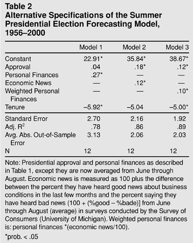
Table 2 presents the revised forecasting model along with a model that uses just the economic news measure and the original forecasting model. The estimates in Table 2 differ from those in the original model in two additional ways: due to limited availability of the economic news variable, the estimates in Table 2 are based on data from 1956 to 2000 instead of 1948 2000, and in an effort to further improve accuracy, all variables are averaged over the summer months (June, July, and August) rather than in the spring.4
The summer measures of the economic variables are based on values for August prior to 1980, and June, July, and August from 1980 to 2000. The one exception to this is 1964 when the data were only available for May.
Table 2 contains several interesting findings. First, of the three models, the unweighted personal finances model (Model 1) has the poorest fit and largest out-of-sample error. Second, the unweighted personal finances model still suggests no significant infl uence from presidential approval. Again, this seems implausible. Third, the economic news (Model 2) and weighted personal finances (Model 3) models are very similar in overall fit, although a slight edge goes to the weighted personal finances model. Another thing that bears mentioning is that both the economic news and weighted personal finances models assign more weight to presidential approval and less weight to the “time for a change” variable than does the unweighted personal finances model.
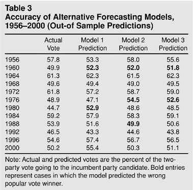
Table 3 presents a summary of the out-of-sample errors from all three models for 1956–2000. Here we see that although Model 1 does as well as Model 3, and better than Model 2, in terms of calling the correct popular vote “winner,” the estimates for Models 2 and 3 are appreciably more on the mark, as was indicated by the mean absolute error in Table 1. The largest error for Model 1 is the 1984 election, which it missed by 8.2 points, while Models 2 and 3 both had their largest error in the 1976 election, missing that outcome by 5.6 and 3.7 points, respectively. Also, focusing on the 2000 outcome, Models 2 and 3 provide very accurate estimates, while the prediction from Model 1 is off by about five percentage points.
A Preliminary 2004 Prediction
Given that the data used to generate the parameters in Table 2 are averaged across June, July, and August, it is not possible to provide a final prediction for the 2004 election at this time (early August). However, assuming that August will not bring a dramatic shift in either presidential approval, economic news, or perceived personal finances, a preliminary estimate based on data from June and July should suffice. Given the June and July values of the predictor variables from the weighed personal finances model (approval=48, weighted personal finances=113.6, tenure=0), the predicted outcome of the 2004 election gives an advantage to President Bush:
Bush % of two-party vote=38.67+(.12*48)+(.10*113.6)−(5.0*0)=55.8
As it happens, the unweighted personal finances model and the economic news model give very similar predictions, 55.5% and 56.6%, respectively, for Bush.
Conclusion
The revised model predicts a victory for George W. Bush. However, this model and its prediction are based on a couple of important assumptions. First, it is assumed that both candidates run effective campaigns that focus on the assets (Bush campaign) and liabilities (Kerry campaign) of the incumbent administration. In other words, voters need to be reminded that the election is about presidential performance. This is how campaigns are normally conducted and there is no reason to expect anything different this year. Second, the model assumes that the values of the key independent variables do not change very much between the time of forecast (early September, once the August data are in) and Election Day. While it is unusual to see wide swings in presidential approval or economic assessments over a two-month period, the 2004 season could hold surprises. Certainly, the volatility of the situation in Iraq could lead to significant changes in the president's approval ratings. And it is also possible that the recent volatility in gasoline prices could swing in one direction or the other and result in a concomitant swing in economic news. Absent these sort of fl uctuations, or other important changes in the context of the election, however, there is no reason to expect the outcome to deviate much from what is predicted.