1. Introduction
Since the advent of high-strength fibres, fibre spinning from polymer melt or concentrated solution at very high extension rates has become increasingly important. In the melt spinning process, the molten polymer extrudate is drawn in to a fibre with exposure to air. The drawn fibre is then quenched in a water bath before being wound on to a rotating spool at the fibre take-up point. The extensional flow field in the air-gap region plays a major role in orienting the polymeric chains along the fibre axis before crystallization or solidification, thus ensuring enhanced mechanical strength of the product fibre. The thinning of the fibre is governed by an extensional flow parameter known as the draw ratio,
 $\mathit{DR}$
, which is the ratio of the velocity at the take-up point (controlled by the speed of the rotating spool) to the velocity of the extrudate at the die-exit point. Thinner, and hence high-strength, fibres are produced by increasing the draw ratio, which in turn implies a higher imposed rate of extension. At a high draw ratio, the extensional flow is known to undergo a hydrodynamic instability which is manifested in the form of sustained periodic oscillations in the fibre cross-section area (Christenen Reference Christenen1962). This instability is widely known as draw resonance, which occurs when the draw ratio exceeds a certain critical value,
 $\mathit{DR}_{c}$
. Following the first reported observation by Christenen (Reference Christenen1962), there have been numerous studies both experimental and theoretical on draw resonance. A very good review of the earlier studies, especially experimental observations, is presented by Petrie & Denn (Reference Petrie and Denn1976).
Theoretical analyses for prediction of the onset of draw resonance are based on stability theory. For isothermal spinning of Newtonian fluids, the onset of draw resonance occurs at a critical draw ratio of 20.218 (Matovich & Pearson Reference Matovich and Pearson1969; Pearson & Matovich Reference Pearson and Matovich1969; Fisher & Denn Reference Fisher and Denn1975a
, Reference Fisher and Denn1976). Hyun (Reference Hyun1978a
) attributed this phenomenon to progression of a kinematic wave, referred to as the throughput wave, along the spinline. By comparing the time required for one complete cycle of a throughput wave to travel the fibre length with the flow residence time, Hyun (Reference Hyun1978a
) predicted the critical value of the draw ratio for a Newtonian fluid to be 19.744, very close to the accurate
 $\mathit{DR}_{c}$
value of 20.218. Under creeping flow and isothermal conditions ignoring gravitational force, this value of
 $\mathit{DR}_{c}$
is independent of the length of the spinning flow (the air gap), the extrudate velocity and the viscosity of the Newtonian fluid.
For polymeric fluids, it is well known that the extensional viscosity, due to its dependence on the deformation rate, plays a significant role in the onset or suppression of draw resonance. For simple power-law fluids, the critical draw ratio is found to depend on the power-law exponent
 $n$
(Hyun Reference Hyun1978b
). For deformation rate thinning fluids (
 $n<1$
),
 $\mathit{DR}_{c}$
drops below 20.2, and it is greater than 20.2 for rate thickening fluids (
 $n>1$
). Real polymeric fluids exhibit complex rheology associated with the state of polymeric chains under deformation. For high-molecular-weight polymers, both rate thinning and rate hardening effects are realized depending upon the flow time scale in comparison to the characteristic relaxation time for polymer chains. Therefore, the viscoelastic model that best describes the rheology of fluid under spinning conditions needs to be analysed for the stability behaviour.
Using a simple viscoelastic model, the Maxwell model, Jung & Hyun (Reference Jung and Hyun1999) found that the critical draw ratio depends on the viscoelasticity characterized by the flow Deborah number, defined as
 $\mathit{De}={\it\lambda}v_{0}/L$
. Here,
 ${\it\lambda}$
is the characteristic relaxation time of the polymer,
 $v_{0}$
is the extrudate velocity through the die exit and
 $L$
is the length of the air gap for the spinning flow. Similar analyses have been carried out for strain-rate-dependent Maxwell fluids (Hyun Reference Hyun1999) and for Phan-Thien-Tanner (PTT) fluids (Lee et al.
Reference Lee, Jung, Hyun and Scriven2005). In these analyses, increase of
 $\mathit{DR}_{c}$
beyond the Newtonian value of 20.2 has been reported due to a rise in extensional viscosity under elongational flow. However, the Maxwell model is not an appropriate description of entangled polymers, the focus of the present study. Moreover, since the Maxwell model is not suitable for extensional flow due to the divergence of the extensional viscosity at a certain Deborah number, the range of
 $\mathit{De}$
covered in previous studies was very limited, and offers insufficient insight for high-strength fibre spinning. One therefore needs to employ a constitutive model which captures the nonlinear extensional rheology of high-molecular-weight polymers. Recently, van der Walt et al. (Reference van der Walt, Hulsen, Bogaerds, Meijer and Bulters2012) employed the eXtended Pom-Pom (XPP) model (Verbeeten, Peters & Baaijens Reference Verbeeten, Peters and Baaijens2001), a variant of the tube model for the dynamics of entangled polymers. The authors studied the linear stability behaviour of spinning under the pull-out condition. Pull-out means that the fibre detaches from within the die (capillary), which occurs when the spinning force is very high. In the present study, we also use the XPP model to examine the finite-amplitude stability behaviour of spinning flow.
For practical applications, it is important to understand the conditions for the onset of draw resonance instability and also the factors that tend to suppress the instability. Since draw resonance originates from the constraints on the fluid velocity at the take-up keeping the air gap fixed, relaxing the constraint helps in suppressing the instability, as found by Renardy (Reference Renardy2007). For the case of polymer melt, the solidification of fibre in the air gap reduces the effective length of the air gap, which tends to stabilize the draw resonance. However, for the case of concentrated polymer solution, significant quenching takes place only in the water bath at the take-up roller, and hence stabilization by non-isothermal spinning may not be realized.
In the present study, we perform a weakly nonlinear stability analysis to predict the dynamical nature of the system under draw resonance conditions. We restrict the analysis to axisymmetric disturbances leading to varicose mode of instability. The disturbance amplitude is finite but small in magnitude, such that the nonlinearities can be expanded in the amplitude series. In the linearly unstable region, the growth of disturbance amplitude is described using the Landau equation
 $\text{d}A/\text{d}t=sA+lA^{3}+\cdots \,$
, where
 $s$
is the linear growth rate and
 $l$
, referred to as the Landau constant, represents the higher-amplitude correction to the linear growth rate (Drazin & Reid Reference Drazin and Reid2004). The formulation of the weakly nonlinear analysis has been developed based on the pioneering work of Stuart (Reference Stuart1956, Reference Stuart1958) and Reynolds & Potter (Reference Reynolds and Potter1967). A similar formulation expanding the perturbation quantities in amplitude series as well as higher harmonics of the fundamental wave has been used to study the nonlinear dynamics in various other problems (Chokshi & Kumaran Reference Chokshi and Kumaran2008a
,Reference Chokshi and Kumaran
b
; Shukla & Alam Reference Shukla and Alam2011). Beyond the transition point, when draw resonance sets in, the finite-amplitude analysis reveals the nature of the bifurcation of the amplitude branch emanating from the transition point. As we increase the draw ratio beyond its critical value,
 $\mathit{DR}_{c}$
, the transition of flow from stable (laminar) to unstable (oscillatory) flow can be either a smooth (supercritical bifurcation) or a sudden (subcritical bifurcation) growth of the disturbance amplitude (Drazin & Reid Reference Drazin and Reid2004). For Newtonian fluids, Fisher & Denn (Reference Fisher and Denn1975b
) found that the bifurcation is supercritical Hopf bifurcation, and the limit cycle behaviour was reported. Numerical simulation of fibre spinning of Newtonian fluid has been performed by Cao (Reference Cao1993), who established a clear mechanism of propagation of a cycle of draw resonance (Cao Reference Cao1991) by capturing spinline profiles at various time instants. For viscoelastic fluids, Yun et al. (Reference Yun, Shin, Lee, Jung and Hyun2008) performed dynamic transient simulations by using the PTT model to understand the supercritical behaviour by resolving the bifurcation diagram. By full numerical simulations, the authors constructed the limit cycles in the linearly unstable region.
The rest of the paper is organized as follows. Section 2 provides the mathematical formulation of the problem that is studied. This section also outlines the theoretical treatment of linear and weakly nonlinear stability analyses. The results of the weakly nonlinear analysis for Newtonian fluid are discussed first in § 3. The findings of the weakly nonlinear analysis are also supported by performing full numerical calculations for Newtonian fluid. Section 4 presents the results of both linear and weakly nonlinear stability analysis for polymeric fluid described by the XPP model. The stability behaviour of the spinning flow is correlated with the nonlinear rheology of the fluid, focusing on the role played by the strain hardening effect. Finally, the important findings are summarized and concluded on in § 5. The governing equations for the sequence of problems studied in the weakly nonlinear analysis are provided in the online supplementary data available at http://dx.doi.org/10.1017/jfm.2015.284.
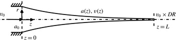
Schematic of the air-gap flow in the fibre spinning process showing the one-dimensional coordinate system. The flow begins at the extrusion point and terminates at the take-up end. The ratio of take-up to extrusion speed is the draw ratio,
 $\mathit{DR}$
.

2. Mathematical model
In the polymer fibre spinning process, a polymer melt or a highly concentrated polymer solution is forced through a spinneret from which a thread is drawn. The threadline undergoes significant thinning aimed at orienting the polymeric chains in the flow direction so as to obtain a fibre with enhanced mechanical strength. The thinning of the fibre takes place in the air gap, as shown in figure 1, at the end of which the fibre is quenched in a water bath and wound onto a take-up roller for further drawing under solid state. The focus of the present study is the flow of polymeric fluid through the air gap. Here, the polymer chains are subjected to uniaxial extensional flow to get a thin fibre with nearly perfectly aligned polymeric chains. For the case of solution spinning, the air-gap flow also promotes evaporation of solvent. We consider the air-gap flow from the die exit (
 $z=0$
) to the take-up point (
 $z=L$
). For polymeric flow, the viscoelastic stresses are dominant, and other forces like inertia, gravity and surface tension are negligible and are hence ignored. For simplicity, isothermal conditions are assumed. The formulation is further simplified by using the slender-body approximation, justifying the one-dimensional model. Hence, all variables, like fibre area, velocity and stresses, are functions of the position along the spinline. The fibre area,
 $a$
, is non-dimensionalized using
 $a_{0}$
, the fibre cross-section area at
 $z=0$
, the velocity,
 $v$
, is non-dimensionalized using
 $v_{0}$
, the velocity at the die exit. The mass and momentum conservation equations are
 $$\begin{eqnarray}\displaystyle & \displaystyle \frac{\partial a}{\partial t}+\frac{\partial (a\boldsymbol{v})}{\partial z}=0, & \displaystyle\end{eqnarray}$$
 $$\begin{eqnarray}\displaystyle & \displaystyle \frac{\partial (aT_{zz})}{\partial z}=0. & \displaystyle\end{eqnarray}$$
 $T_{zz}$
is the total normal stress in the
 $z$
direction, which is given by the first normal stress difference
 $({\it\tau}_{zz}-{\it\tau}_{rr})$
. The momentum conservation equation (2.2) implies that the spinning force given by
 $F=aT_{zz}$
is constant along the spinline.
For closure, the above governing equations need to be supplemented with a constitutive equation relating the stresses in the fluid to the rate of deformation. The emphasis of the present analysis is on the spinning process for high-strength polymer fibre. For this case, the polymeric chains are of very high molecular weight, leading to entanglement of chains. It is well known that the dynamics of entangled long chains is very different from that for unentangled short chains. Hence, the simplest Maxwell-type constitutive equations are not appropriate to capture the restricted motion, known as reptation, of the entangled polymers. The rheology of the entangled polymers is best described by a tube model (Doi & Edwards Reference Doi and Edwards1978), wherein the polymeric chains are assumed to be confined in a tube-like region formed by the presence of topological constraints by the neighbouring chains. Many variants of the classical tube model have been developed to describe the nonlinear rheology of polymeric melt. In the present study, we adopt one such variant of the classical tube model, the XPP model (Verbeeten et al. Reference Verbeeten, Peters and Baaijens2001). The XPP model considers a polymeric chain to be composed of two parts, a backbone chain and free dangling arms present at each end of the backbone. To reptate, a chain must retract the branches to the retraction point (local branch point). This model is selected as it best describes the rheology of polymeric fluid under a strong rate of deformation. Most importantly, the XPP model exhibits the strain hardening effect in polymers, which is an essential property of fluids for fibre spinning applications. The constitutive equation for the XPP model in dimensionless form is given as
 $$\begin{eqnarray}\displaystyle & \displaystyle \frac{\partial {\it\tau}}{\partial t}+\boldsymbol{v}\boldsymbol{\cdot }\boldsymbol{{\rm\nabla}}{\it\tau}-{\it\tau}\boldsymbol{\cdot }(\boldsymbol{{\rm\nabla}}\boldsymbol{v})-(\boldsymbol{{\rm\nabla}}\boldsymbol{v})^{\text{T}}\boldsymbol{\cdot }{\it\tau}=[(\boldsymbol{{\rm\nabla}}\boldsymbol{v})+(\boldsymbol{{\rm\nabla}}\boldsymbol{v})^{\text{T}}]-\frac{[F{\it\tau}+(F-1)\boldsymbol{I}]}{\mathit{De}}, & \displaystyle\end{eqnarray}$$
 $$\begin{eqnarray}\displaystyle & \displaystyle F=2r\left(1-\frac{1}{{\it\Lambda}}\right)\exp \left[\frac{2}{q}({\it\Lambda}-1)\right]+\frac{1}{{\it\Lambda}^{2}}, & \displaystyle\end{eqnarray}$$
 $$\begin{eqnarray}\displaystyle & \displaystyle {\it\Lambda}^{2}=1+{\textstyle \frac{1}{3}}\text{tr}({\it\tau}). & \displaystyle\end{eqnarray}$$
 ${\it\tau}$
is made dimensionless using the shear modulus of the fluid,
 $G$
. The superscript T denotes transpose. The term
 ${\it\Lambda}$
is a measure of the extent of chain stretch, and it is defined as the ratio of polymer chain size under flow to that under equilibrium. The terms
 $r$
and
 $q$
are parameters of the XPP model,
 $r$
representing the ratio of relaxation times for backbone orientation to backbone stretch, and
 $q$
denoting the number of free arms branching at each end of the backbone chain. The term
 $\mathit{De}$
is the Deborah number, defined as
 $\mathit{De}={\it\lambda}v_{0}/L$
, where
 ${\it\lambda}$
is the longest relaxation time of the XPP molecule (i.e. the orientation relaxation time for the backbone chain). The Deborah number is the measure of fluid elasticity, such that for
 $\mathit{De}\ll 1$
, the polymer chains are neither stretched nor oriented, and hence the fluid behaves like a Newtonian fluid.
Due to the inherent characteristics of the XPP model, the idealized molecule first experiences a stretch, followed by orientation as the strain rate increases; hence, a complex behaviour is expected as
 $\mathit{De}$
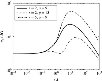
increases. The extensional behaviour of the XPP model is shown in figure 2, in which the steady-state extensional viscosity (non-dimensionalized by the shear viscosity) is plotted against the extension rate (non-dimensionalized using the relaxation time,
 ${\it\lambda}$
) for a uniaxial extensional flow. At low extension rates, the extensional viscosity is equal to 3, which is the Trouton’s ratio for Newtonian fluids. As the extension rate increases, stretching of the backbone chain is caused by the branch point, leading to strain hardening. At an even higher extension rate, the arms retract to the branch point, thus releasing the backbone stretch, indicated by a drop in the extensional viscosity. In figure 2 there are two peaks, separated by the relaxation time factor,
 $r$
. For extension rates between these two peaks, there is a small drop in
 ${\it\eta}_{e}$
due to the orientation of the chains in the flow direction. Typically, the first peak occurs at a strain rate of approximately
 ${\it\lambda}^{-1}$
, whereas the second peak occurs at a strain rate of approximately
 $r{\it\lambda}^{-1}$
. For small values of
 $r$
, the peaks are close and are indistinguishable.
Non-dimensionalized extensional viscosity plotted against dimensionless extension rate for the XPP model using the parameters
 $r=2$
and different values of
 $q$
. Beginning with the Trouton’s ratio for Newtonian fluids (
 $T_{r}=3$
), the viscosity undergoes strain rate hardening followed by softening at high extension.

The governing equations (2.1)–(2.3) are supplemented with the boundary conditions
 $$\begin{eqnarray}\displaystyle \text{at}\quad z=0: & & \displaystyle \;a=1,~v=1,~{\it\tau}_{rr}=0,\end{eqnarray}$$
 $$\begin{eqnarray}\displaystyle \text{at}\quad z=1: & & \displaystyle \;v=\mathit{DR}.\end{eqnarray}$$
2.1. Linear stability analysis
The steady-state solution for the fibre profile,
 $\bar{a}(z)$
and
 $\bar{v}(z)$
, is analysed for stability to infinitesimal amplitude disturbances. In linear stability analysis, the base-state solution is superimposed with one-dimensional axisymmetric perturbations of the following form:
 $$\begin{eqnarray}{\it\phi}(z,t)=\bar{{\it\phi}}(z)+A\,\tilde{{\it\phi}}(z)\,\text{e}^{st},\end{eqnarray}$$
where a general variable
 ${\it\phi}$
represents the variable for the fibre,
 ${\it\phi}=[a,v,{\it\tau}_{zz},{\it\tau}_{rr}]^{\text{T}}$
. Here,
 $\bar{{\it\phi}}(z)$
represents the steady-state variable and
 $A$
indicates the amplitude of the infinitesimally small amplitude disturbance;
 $\tilde{{\it\phi}}(z)$
is the axial profile of the axisymmetric disturbance variable
 ${\it\phi}$
. Here,
 $s$
is the complex-valued growth rate for the disturbance, given by
 $s=s_{r}+\text{i}s_{i}$
. The real part,
 $s_{r}$
, represents the growth or decay of the disturbance amplitude and the imaginary part,
 $s_{i}$
, provides the frequency part of the travelling wave disturbance. For draw ratios below the critical value,
 $\mathit{DR}_{c}$
, the disturbance growth rate
 $s_{r}$
is negative, and it is positive for
 $\mathit{DR}>\mathit{DR}_{c}$
. Thus, by setting the condition for neutral stability,
 $s_{r}=0$
, one can estimate the critical value of the draw ratio,
 $\mathit{DR}_{c}$
. The abovementioned form for the one-dimensional axisymmetric disturbance has been employed earlier for both Newtonian fluids (Pearson & Matovich Reference Pearson and Matovich1969) and Maxwell-type viscoelastic fluids (Jung & Hyun Reference Jung and Hyun1999).
In linear stability analysis, the superposition (2.8) is substituted in the flow governing equations and the resultant equations are linearized by retaining the terms of the order of
 $O(A)$
, leading to the governing equations for the disturbance as follows:
 $$\begin{eqnarray}\displaystyle & \displaystyle s\tilde{a}+\bar{a}\frac{\text{d}\tilde{v}}{\text{d}z}+\tilde{a}\frac{\text{d}\bar{v}}{\text{d}z}+\bar{v}\frac{\text{d}\tilde{a}}{\text{d}z}+\tilde{v}\frac{\text{d}\bar{a}}{\text{d}z}=0, & \displaystyle\end{eqnarray}$$
 $$\begin{eqnarray}\displaystyle & \displaystyle (\tilde{{\it\tau}}_{zz}-\tilde{{\it\tau}}_{rr})\frac{\text{d}\bar{a}}{\text{d}z}+\bar{a}\frac{\text{d}}{\text{d}z}(\tilde{{\it\tau}}_{zz}-\tilde{{\it\tau}}_{rr})+(\bar{{\it\tau}}_{zz}-\bar{{\it\tau}}_{rr})\frac{\text{d}\tilde{a}}{\text{d}z}+\tilde{a}\frac{\text{d}}{\text{d}z}(\bar{{\it\tau}}_{zz}-\bar{{\it\tau}}_{rr})=0, & \displaystyle\end{eqnarray}$$
 $$\begin{eqnarray}\displaystyle & \displaystyle s\tilde{{\it\tau}}_{zz}+\bar{v}\frac{\text{d}\tilde{{\it\tau}}_{zz}}{\text{d}z}+\tilde{v}\frac{\bar{{\it\tau}}_{zz}}{\text{d}z}-2(\bar{{\it\tau}}_{zz}+1)\frac{\text{d}\tilde{v}}{\text{d}z}-2\tilde{{\it\tau}}_{zz}\frac{\text{d}\bar{v}}{\text{d}z}+\frac{\bar{F}\tilde{{\it\tau}}_{zz}+\tilde{F}(\bar{{\it\tau}}_{zz}+1)}{\mathit{De}}=0, & \displaystyle\end{eqnarray}$$
 $$\begin{eqnarray}\displaystyle & \displaystyle s\tilde{{\it\tau}}_{rr}+\bar{v}\frac{\text{d}\tilde{{\it\tau}}_{rr}}{\text{d}z}+\tilde{v}\frac{\bar{{\it\tau}}_{rr}}{\text{d}z}+(\bar{{\it\tau}}_{rr}+1)\frac{\text{d}\tilde{v}}{\text{d}z}+\tilde{{\it\tau}}_{rr}\frac{\text{d}\bar{v}}{\text{d}z}+\frac{\bar{F}\tilde{{\it\tau}}_{rr}+\tilde{F}(\bar{{\it\tau}}_{rr}+1)}{\mathit{De}}=0, & \displaystyle\end{eqnarray}$$
 $$\begin{eqnarray}\displaystyle & \displaystyle \tilde{F}=\tilde{{\it\Lambda}}^{2}\left[-\frac{1}{\bar{{\it\Lambda}}^{4}}+\left(\frac{1}{2\,\bar{{\it\Lambda}}^{3}}-\frac{1}{q\,\bar{{\it\Lambda}}^{2}}+\frac{1}{q\,\bar{{\it\Lambda}}}\right)\,2\,r\,\text{exp}\left(\frac{2(\bar{{\it\Lambda}}-1)}{q}\right)\right], & \displaystyle\end{eqnarray}$$
 $$\begin{eqnarray}\displaystyle & \displaystyle \tilde{{\it\Lambda}}=\frac{\tilde{{\it\tau}}_{zz}+2\,\tilde{{\it\tau}}_{rr}}{6\,\bar{{\it\Lambda}}}. & \displaystyle\end{eqnarray}$$
 $$\begin{eqnarray}\displaystyle & & \displaystyle \text{at}\quad z=0:\quad \tilde{a}=0,~\tilde{v}=0,~\tilde{{\it\tau}}_{rr}=0,\end{eqnarray}$$
 $$\begin{eqnarray}\displaystyle & & \displaystyle \text{at}\quad z=1:\quad \tilde{v}=0.\end{eqnarray}$$
 $s$
, as the eigenvalue of the disturbance problem. By setting
 $s_{r}=0$
, the critical draw ratio
 $\mathit{DR}_{c}$
is calculated for a given value of the Deborah number. The linear stability behaviour of the fibre spinning problem is presented in the form of a neutral stability diagram in the
 $\mathit{DR}_{c}$
–
 $\mathit{De}$
plane.
2.2. Weakly nonlinear stability analysis
The linear stability analysis provides the critical point for the flow transition,
 $\mathit{DR}_{c}$
, beyond which the draw resonance sets in. In the unstable regime,
 $\mathit{DR}>\mathit{DR}_{c}$
, any disturbance, even if infinitesimally small at the beginning, grows exponentially with time. However, as the amplitude of the disturbance becomes finite, the nonlinear terms ignored in the linear stability analysis become significant and the exponential linear growth rate is modified by the nonlinearities in the governing equations. For practical applications, in addition to the knowledge of the flow transition point, it is essential to know the amplitude of the oscillations in the fibre cross-section area in the regime beyond the transition point. The estimation of the amplitude is beyond the scope of linear stability theory and one needs to carry out finite-amplitude stability analysis. In this section, we briefly discuss the weakly nonlinear stability analysis.
The steady-state profile is superimposed with a transient disturbance as follows:
 $$\begin{eqnarray}{\it\phi}(z,t)=\bar{{\it\phi}}(z)+{\it\phi}^{\prime }(z,t).\end{eqnarray}$$
In finite-amplitude analysis, the perturbation field
 ${\it\phi}^{\prime }(z,t)$
is expanded in power series of amplitude
 $A_{0}(t)$
as well as in higher-order harmonics of the fundamental disturbance wave (Reynolds & Potter Reference Reynolds and Potter1967). The fundamental mode is, in fact, the solution of the linear stability problem,
 $\tilde{{\it\phi}}(z)$
. The dynamical equation for the complex-valued amplitude
 $A_{0}(t)$
assumes the form of a Landau equation:
 $$\begin{eqnarray}\frac{\text{d}A_{0}}{\text{d}t}=s\,A_{0}+m\,A_{0}^{2}+l\,A_{0}^{3}+\cdots \,.\end{eqnarray}$$
Here,
 $s$
is the growth rate from linear stability theory and the coefficients
 $m$
and
 $l$
are higher-order corrections to the linear growth rate and are termed as Landau constants. As will be discussed later, the coefficients of the terms containing even powers of
 $A_{0}$
vanish. Hence, in the truncated Landau equation (2.18), the coefficient
 $m$
turns out to be identically zero, and the Landau constant
 $l$
, a complex-valued quantity, represents an
 $O(A_{0}^{2})$
correction to the linear growth rate. Here, the amplitude
 $A_{0}(t)$
is a complex-valued quantity, containing the transients of both the magnitude and the phase of the disturbance amplitude. Thus, we may write
 $A_{0}(t)=A_{1}(t)\,\text{e}^{\text{i}{\it\omega}t}$
, where
 $A_{1}=|A_{0}|$
, the magnitude of the perturbation amplitude, a real-valued quantity. It can be easily shown that the governing equations for the absolute magnitude and frequency of disturbance are given by
 $$\begin{eqnarray}\displaystyle & \displaystyle \frac{1}{A_{1}}\frac{\text{d}A_{1}}{\text{d}t}=s_{r}+l_{r}\,A_{1}^{2}+\cdots \,, & \displaystyle\end{eqnarray}$$
 $$\begin{eqnarray}\displaystyle & {\it\omega}=s_{i}+l_{i}\,A_{1}^{2}+\cdots \,. & \displaystyle\end{eqnarray}$$
 $s=s_{r}+\text{i}s_{i}$
and the Landau constant
 $l=l_{r}+\text{i}l_{i}$
. The above expressions hold for weakly nonlinear problem, such that the amplitude is finite but small in magnitude,
 $A_{1}\ll 1$
. We take
 $A_{1}(t)={\it\epsilon}A(t)$
, where
 ${\it\epsilon}$
represents the order of magnitude of the amplitude, the small parameter in the expansion, and
 $A(t)\sim O(1)$
. It should be noted that
 $A(t)$
is a real quantity.
The expansion of the disturbance variable
 $\tilde{{\it\phi}}$
in (2.17) is as follows:
 $$\begin{eqnarray}{\it\phi}^{\prime }(z,t)=\mathop{\sum }_{k=0}^{\infty }\mathop{\sum }_{\begin{array}{@{}c@{}}n=k\\ n\neq 0\end{array}}^{\infty }({\it\epsilon}A(t))^{n}\,[\text{e}^{kst}\tilde{{\it\phi}}^{(k,n)}(z)+\text{e}^{-kst}\tilde{{\it\phi}^{\dagger }}^{(k,n)}(z)].\end{eqnarray}$$
Here,
 $\tilde{{\it\phi}}^{(k,n)}$
is the disturbance eigenfunction with harmonic index
 $k$
and amplitude power
 $n$
. The superscript
 $\dagger$
denotes complex conjugate. The framework of the weakly nonlinear analysis is valid only in the vicinity of the transition point, so that
 $|\mathit{DR}-\mathit{DR}_{c}|\ll 1$
. In the neighbourhood of
 $\mathit{DR}_{c}$
, the linear growth rate takes the form
 $$\begin{eqnarray}s=\frac{\text{d}s}{\text{d}\mathit{DR}}\,(\mathit{DR}-\mathit{DR}_{c}),\end{eqnarray}$$
with real part
 $$\begin{eqnarray}s_{r}=\frac{\text{d}s_{r}}{\text{d}\mathit{DR}}\,(\mathit{DR}-\mathit{DR}_{c}).\end{eqnarray}$$
In order to establish a balance between the two terms on the right-hand side of the Landau equation (2.19), the order of magnitude of the linear growth rate
 $s_{r}$
should be
 $O({\it\epsilon}^{2})$
, since
 $A_{1}\sim O({\it\epsilon})$
and assuming the Landau constant
 $l\sim O(1)$
. Thus, from (2.23), the order of magnitude of
 $(\mathit{DR}-\mathit{DR}_{c})$
should be
 $O({\it\epsilon}^{2})$
, as
 $(\text{d}s_{r}/\text{d}\mathit{DR})\sim O(1)$
. For definiteness, we denote
 $(\mathit{DR}-\mathit{DR}_{c})=\mathit{DR}_{2}{\it\epsilon}^{2}$
, where
 $\mathit{DR}_{2}\sim O(1)$
. Now, the balance between the right- and left-hand sides of the amplitude (2.19) is achieved by taking
 $(1/A_{1})(\text{d}A_{1}/\text{d}t)$
to be of the order of
 $O(eps^{2})$
. Therefore, we introduce a slow time scale
 ${\it\tau}$
such that the time derivative
 $\text{d}/\text{d}t$
is expanded as
 $\text{d}/\text{d}t+{\it\epsilon}^{2}\,\text{d}/\text{d}{\it\tau}$
, with the first term being
 $O(1)$
and the second term
 $O({\it\epsilon}^{2})$
(Chokshi & Kumaran Reference Chokshi and Kumaran2008a
). Henceforth, the time
 $t$
indicates the fast time scale, corresponding to the inverse of the frequency of oscillations, and the time
 ${\it\tau}$
denotes the slow time scale, corresponding to the rate of growth or decay of the disturbance amplitude. This leads to the definition of the disturbance amplitude as
 $A({\it\tau})$
. Thus, the dynamical equation for the amplitude (2.19) scaled at order
 $O({\it\epsilon}^{2})$
becomes
 $$\begin{eqnarray}\frac{1}{A({\it\tau})}\frac{\text{d}A}{\text{d}{\it\tau}}=\frac{\text{d}s_{r}}{\text{d}\mathit{DR}}\mathit{DR}_{2}+l_{r}\,A({\it\tau})^{2}+\cdots \,.\end{eqnarray}$$
Here,
 $A({\it\tau})$
represents the variation of the disturbance amplitude with the slow time scale
 ${\it\tau}$
. The higher-order correction to the frequency of the fundamental disturbance wave due to nonlinear interactions as in (2.20) becomes
 $$\begin{eqnarray}{\it\omega}=s_{i}+\frac{\text{d}s_{i}}{\text{d}\mathit{DR}}\mathit{DR}_{2}+l_{i}\,A({\it\tau})^{2}+\cdots \,.\end{eqnarray}$$
In weakly nonlinear analysis, we calculate the Landau constant
 $l=l_{r}+\text{i}l_{i}$
. The sign of the real part of the Landau constant reveals the nature of the bifurcation at the transition point. For
 $l_{r}<0$
, the nonlinearities tend to stabilize the amplitude growth. In this case, above the transition point (
 $\mathit{DR}>\mathit{DR}_{c}$
) the exponential growth of the disturbance amplitude is stabilized by nonlinear self-interaction of the fundamental mode, and the amplitude saturates to an equilibrium value
 $A_{e}$
, which is obtained as the fixed point of the dynamical equation (2.24). Thus, for
 $l_{r}<0$
, the flow is said to undergo a supercritical bifurcation at the transition point. On the contrary, for
 $l_{r}>0$
, the nonlinearities tend to destabilize the flow and it can become unstable even below the transition point (
 $\mathit{DR}<\mathit{DR}_{c}$
) provided that the imposed disturbance amplitude is greater than a certain threshold value
 $A_{th}$
. Therefore, the finite-amplitude manifold is of subcritical nature in the vicinity of the transition point.
The fixed point of the amplitude (2.24) gives an equilibrium amplitude from which the finite-amplitude branch can be constructed. By setting the rate of change of the amplitude to zero, the equilibrium or threshold amplitude is given as
 $$\begin{eqnarray}A=\sqrt{-\frac{s_{r}}{l_{r}}}.\end{eqnarray}$$
This relation should be the same for both the equilibrium (for the supercritical branch) as well as the threshold amplitude (for the subcritical branch), since
 $s_{r}$
and
 $l_{r}$
are always of opposite signs in the region of interest. The methodology to calculate the Landau constant and the disturbance equations at various amplitude orders is outlined in the supplementary material.
3. Validation for Newtonian fluids
It is well known that for Newtonian fluids, the critical value of the draw ratio for the onset of instability is
 $\mathit{DR}_{c}=20.218$
, which is independent of the fluid viscosity, the flow rate and the air gap (Pearson & Matovich Reference Pearson and Matovich1969). In the vicinity of the transition point, the spinning flow is known to exhibit a supercritical amplitude branch (Fisher & Denn Reference Fisher and Denn1975b
; Schultz et al.
Reference Schultz, Zebib, Davis and Lee1984). With the objective of validating our methodology outlined in § 2.2, we calculate the Landau constant in the neighbourhood of the critical point. The fundamental wave is the solution of the linear stability problem and is denoted as
 $\tilde{{\it\phi}}^{(1,1)}$
, with harmonic index
 $k=1$
and amplitude order
 $n=1$
. It is important to note that in order to obtain the eigenfunction for the (1,1) problem, we have to provide an additional normalization condition. Throughout the paper, we employ a normalization condition
 $\tilde{a}^{(1,1)}|_{z=0}=1$
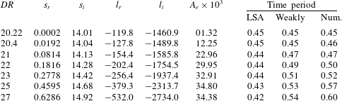
. Table 1 tabulates the calculated values of the Landau constant,
 $l$
, for
 $\mathit{DR}>\mathit{DR}_{c}$
. As is seen, the real part of the Landau constant,
 $l_{r}$
, is negative. Thus, the finite-amplitude branch exhibits a supercritical bifurcation at the transition point,
 $\mathit{DR}=\mathit{DR}_{c}$
. By setting
 $\text{d}A/\text{d}{\it\tau}=0$
in the Landau equation (2.26), we calculate the amplitude of the stationary state post-transition as tabulated in table 1.
The Landau constant,
 $l$
, for the Newtonian fluid, calculated for
 $\mathit{DR}>\mathit{DR}_{c}$
. The equilibrium amplitude,
 $A_{e}$
, and the time period of the unstable disturbance are also tabulated. The time period is calculated using linear stability analysis (LSA), weakly nonlinear stability analysis (Weakly) and full numerical simulation (Num.).

In addition to the higher-order correction to the linear growth rate, the weakly nonlinear analysis also provides the higher-order correction to the frequency of the disturbance wave, calculated using (2.25). The time period for disturbance, made non-dimensional using the flow time scale
 $L/v_{0}$
, is given by
 $2{\rm\pi}/{\it\omega}$
. In table 1, the time periods are tabulated using three approaches. Here, LSA stands for the time period obtained from linear stability analysis (
 $2{\rm\pi}/s_{i}$
). This is corrected by weakly nonlinear analysis. Finally, we also obtain the time period from the full numerical solution. In the vicinity of the critical point, the time periods calculated by the three methods are the same. For
 $\mathit{DR}>\mathit{DR}_{c}$
, the linear analysis predicts that the time period decreases as the draw ratio increases. However, the experiments by Demay & Agassant (Reference Demay and Agassant1985) find that the time period, in fact, increases with increasing draw ratio. The weakly nonlinear analysis correctly predicts this trend, and the value is similar to that obtained from full numerical calculations.
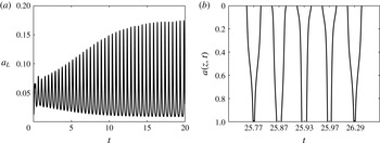
In the full numerical solution, we numerically integrate the governing equations (2.1) and (2.2) in time, and the transient of the imposed disturbance is studied. We employ the orthogonal collocation technique for discretization in space and the Crank–Nicolson method for integration in time. The steady-state fibre area profile is perturbed by introducing a small-amplitude periodic disturbance. Under the unstable spinning conditions at
 $\mathit{DR}=22$
, figure 3(a) shows that the disturbance in the take-up area initially grows exponentially and then saturates to an equilibrium amplitude while undergoing periodic oscillations. In the periodic steady state, the deviation in the take-up area from its steady-state value may be measured in terms of
 $a_{max}^{\prime }=a_{L}-\bar{a}|_{z=1}$
or
 $a_{min}^{\prime }=\bar{a}|_{z=1}-a_{L}$
, the perturbations to maximum and minimum area respectively. Here, the steady-state value
 $\bar{a}_{z=1}=1/\mathit{DR}$
. Figure 3(b) shows snapshots of the fibre cross-section area at different times after the steady oscillatory state is reached. The figure clearly shows a throughput wave propagating through the fibre, a state known as draw resonance. Since the supercritically stable state is a periodic solution, the supercritical manifold shows a limit cycle behaviour (Fisher & Denn Reference Fisher and Denn1975b
; Schultz et al.
Reference Schultz, Zebib, Davis and Lee1984).
Transient take-up area obtained from full numerical calculations for
 $\mathit{DR}=22>\mathit{DR}_{c}$
. (a) The steady-state profile is perturbed by a small-amplitude sinusoidal wave. After initial exponential growth, the amplitude saturates to an equilibrium state due to nonlinear interactions. (b) Snapshots of the fibre cross-section area at different times. The transient evolution of the spinline profile clearly shows a travelling wave propagating through the fibre.

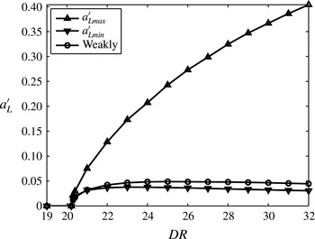
Figure 4 plots the numerically obtained
 $a_{max}^{\prime }$
and
 $a_{min}^{\prime }$
corresponding to the equilibrium state as a function of
 $\mathit{DR}$
. Using the equilibrium amplitude
 $A_{e}$
from weakly nonlinear analysis, we plot the same quantity,
 $a^{\prime }$
. The area amplitude branch from the weakly nonlinear analysis is found to be quantitatively comparable to the minimum area deviation branch from the full numerical simulation.
Maximum and minimum take-up area deviations from the steady-state value plotted as a function of draw ratio. For comparison, the equilibrium amplitude for the take-up area disturbance as obtained from the weakly nonlinear stability analysis is also plotted.

4. Results and discussion – polymeric fluid
4.1. Linear stability analysis
Viscoelastic fluid, described using the XPP model, introduces three additional parameters, namely the flow Deborah number, a measure of the fluid elasticity,
 $q$
, the number of arms at each branch point in an idealized XPP molecule (a measure of the extent of the strain hardening effect), and
 $r$
, the ratio of the backbone orientation to the stretch relaxation times. The magnitude of the parameter
 $r$
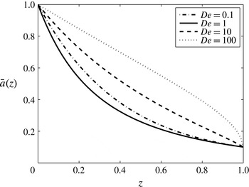
governs the separation of time scales for two different modes of stress relaxation in polymeric chains. The steady-state solution of the governing equations (2.1)–(2.3) is obtained numerically. The steady-state profile of the fibre cross-section area,
 $\bar{a}(z)$
, which forms the base state for the stability analysis, is shown in figure 5.
The steady-state profile of the fibre cross-section area,
 $\bar{a}(z)$
, for
 $\mathit{DR}=10$
and different values of the Deborah number. The XPP parameters are
 $r=2,q=9$
.

Next, the linear stability analysis is carried out following the procedure outlined in § 2.1, and the critical value of the draw ratio,
 $\mathit{DR}_{c}$
, is obtained by setting the real part of the growth rate
 $s_{r}=0$
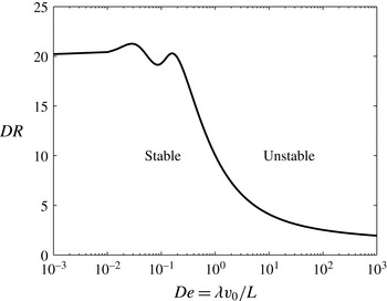
. Figure 6 plots the neutral stability diagram and shows the effect of the Deborah number on
 $\mathit{DR}_{c}$
for
 $r=2$
and
 $q=9$
. In the limit
 $\mathit{DR}\rightarrow 0$
, the value of
 $\mathit{DR}_{c}=20.218$
for Newtonian fluid is recovered. The region below the neutral stability diagram indicates stable spinning, whereas that above the curve represents draw resonance of the fibre, i.e. spinning with periodic oscillation in the fibre cross-section area. The variation of
 $\mathit{DR}_{c}$
with
 $\mathit{De}$
shows two peaks corresponding to two relaxation times associated with the polymer chain. The ratio of Deborah numbers corresponding to the two peaks is related to the parameter
 $r$
. Around the range of Deborah numbers for the two peaks, the backbone chain undergoes stretching caused by the extensional flow, and stretch relaxation is prevented by the branch points. This leads to enhancement in the extensional viscosity of the fluid (refer to figure 2), leading to a stabilizing effect, indicated by an increasing trend in
 $\mathit{DR}_{c}$
. For Deborah number values beyond the second peak, the arms at the branch points have retracted to the branch points, and the chains orient in the flow direction, resulting in decrease in the extensional viscosity, as shown in figure 2. This strain softening leads to destabilization, indicated by decrease in
 $\mathit{DR}_{c}$
with Deborah number, in the regime of fast flows with
 $\mathit{De}\gg 1$
. A similar stability diagram has recently been constructed by van der Walt et al. (Reference van der Walt, Hulsen, Bogaerds, Meijer and Bulters2012).
Variation in the critical draw ratio with the flow Deborah number
 $\mathit{De}$
using
 $r=2$
and
 $q=9$
. The region below the neutral stability curve indicates stable flow and that above the curve represents linearly unstable flow.

The polymeric systems for practical application of spinning to produce high-strength fibres exhibit extensive strain hardening effects for a range of strain rates. In the XPP model, increase of the value of the parameter
 $q$
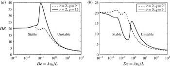
(which means a greater number of arms to retract before reptation) gives the desired strain hardening effect. The role of the strain hardening parameter is depicted in figure 7(a). It is seen that increase of
 $q$
tends to enhance the peak value of
 $\mathit{DR}_{c}$
to well above the Newtonian value of 20.218, confirming the stabilizing effect of strain hardening in extensional flow. Interestingly, there exists a strong correlation between the nonlinear extensional rheology and the stability behaviour. Similarly, increase of the parameter
 $r$
would mean increased separation between the two peaks in the stability map. The role of the parameter
 $r$
in the stability diagram is shown in figure 7(b). Here, due to the separation of the relaxation time scales, the two peaks in
 $\mathit{DR}_{c}$
separate further.
Variation in the critical draw ratio with the flow Deborah number
 $\mathit{De}$
. (a) The effect of the strain hardening parameter,
 $q$
, is shown for the parameter
 $r=2$
. A greater number of free arms increases the peak
 $\mathit{DR}_{c}$
due to enhancement in extensional viscosity. (b) The effect of the relaxation time ratio,
 $r$
, for
 $q=9$
. Two peaks are distinguishable due to the separation in time scales for stretch and orientation relaxation.

It is important to note that for rheologically different polymers, the model parameters need to be fitted from both linear and nonlinear rheology measurements. The measurements include the oscillatory frequency sweep to determine the plateau modulus,
 $G$
, and the longest relaxation time,
 ${\it\lambda}$
, and transient uniaxial extension rheometry to obtain the parameters characterizing the extent of strain hardening,
 $r$
and
 $q$
. For example, from a certain data set available from rheological experimentation on a sample of high-molecular-weight polyethylene (
 $M_{w}\approx 10^{5}~\text{g}~\text{mol}^{-1}$
) by Auhl et al. (Reference Auhl, Hoyle, Hassell, Lord and Harlen2011), we fit the data using the tool REPTATE (Likhtman & Ramirez Reference Likhtman and Ramirez2009) and find typical values for the model parameters as tabulated in table 2.
Typical values of the XPP model parameters for high-molecular-weight polymers.

4.2. Weakly nonlinear analysis
The linear stability theory predicts the transition point depicted as a stability diagram in the
 $\mathit{DR}_{c}$
–
 $\mathit{De}$
plane, as shown in figure 6. In the unstable region of the diagram (above the neutral stability curve), the theory predicts draw resonance which is manifested in the form of periodic oscillations in the fibre cross-section area. However, the severity of draw resonance, quantified in terms of the amplitude of area variations, cannot be predicted from the linear theory. In § 3, we have found that, for a Newtonian fluid, the finite-amplitude bifurcation at the transition point is supercritical in nature, and corresponding equilibrium amplitude of the draw resonance is also estimated. For viscoelastic fluids, we perform a weakly nonlinear stability analysis to address the following pertinent questions. Does the bifurcation remain supercritical for viscoelastic fluids? What is the role of fluid elasticity in the severity of draw resonance?
The finite-amplitude analysis is carried out in the vicinity of the neutral stability diagram in figure 6, and the Landau constant is calculated for different values of the flow Deborah number. For small values of
 $\mathit{De}$
, the real part of the Landau constant,
 $l_{r}$
, remains negative, indicating a supercritical bifurcation for
 $\mathit{De}\ll 1$
. In this regime, we calculate the equilibrium amplitude and construct a finite-amplitude manifold emerging from
 $\mathit{DR}=\mathit{DR}_{c}$
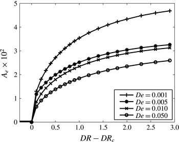
, as shown in figure 8. In order to compare
 $A_{e}$
for different values of the Deborah number for which the values of
 $\mathit{DR}_{c}$
are different, we plot
 $A_{e}$
against
 $\mathit{DR}-\mathit{DR}_{c}$
, so that amplitude curves for different values of
 $\mathit{De}$
originate from a single point. Upon increasing the Deborah number, the magnitude of
 $l_{r}$
increases, with the sign remaining negative, indicating an increasingly stabilizing role of nonlinearities. Therefore, the equilibrium amplitude,
 $A_{e}$
, is found to decrease with increasing elasticity, meaning that the amplitude of the temporal oscillations is less pronounced in the regime
 $\mathit{De}\ll 1$
. This happens due to globular polymeric chains being stretched by elongational flow, offering a resistance to increasing strain rate. This stabilizing role of elasticity due to nonlinear interactions is in line with the linear stability finding, where
 $\mathit{DR}_{c}$
is found to attain a distinguishable peak for moderate values of the Deborah number.
Equilibrium amplitude as a function of draw ratio (
 $\mathit{DR}-\mathit{DR}_{c}$
) in the low-Deborah-number range. The amplitude curves drop from the Newtonian curve. The draw resonance behaviour is less pronounced for viscoelastic fluids, indicating increasing stability. The XPP parameters are
 $r=2$
and
 $q=9$
.

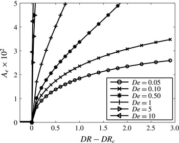
On further increasing the fluid elasticity, the trend reverses. The magnitude of
 $l_{r}$
decreases, with the sign remaining negative. Thus, the equilibrium amplitude is found to increase with increase in
 $\mathit{De}$
, as shown in figure 9. In this regime, the draw resonance becomes more intense as the stabilizing contribution of the nonlinear self-interaction of the fundamental wave diminishes. Interestingly, for this range of Deborah number (
 $\mathit{De}>0.1$
), the reduction in extensional viscosity due to chain orientation has been shown to decrease
 $\mathit{DR}_{c}$
(refer to figure 6). Hence, the destabilizing role of strain softening is observed for both infinitesimally-small-amplitude and finite-amplitude disturbances.
Equilibrium amplitude as a function of draw ratio (
 $\mathit{DR}-\mathit{DR}_{c}$
) in the moderate-Deborah-number range. The amplitude curves rise rapidly, indicating the destabilizing role of fluid elasticity. The XPP parameters are
 $r=2$
,
 $q=9$
.

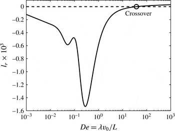
Variation in the real part of the Landau constant,
 $l_{r}$
, calculated at
 $\mathit{DR}=\mathit{DR}_{c}$
, with the flow Deborah number. The system displays maximum supercriticality at the lowest point
 $\mathit{De}\approx 0.3$
. At higher
 $\mathit{De}$
the Landau constant approaches zero. At this point,
 $\mathit{De}\approx 40$
, the bifurcation at the flow transition point crosses over from supercritical to subcritical nature. The XPP parameters are
 $r=2$
and
 $q=9$
.

Interestingly, the value of the real part of the Landau constant along the amplitude manifold for any value of
 $\mathit{De}$
decreases and approaches zero as
 $\mathit{DR}$
increases beyond
 $\mathit{DR}_{c}$
. At some high value of
 $\mathit{DR}$
,
 $l_{r}$
becomes zero, at which point the amplitude branch turns back and the supercritical region ends. Therefore, for a certain high value of
 $\mathit{DR}-\mathit{DR}_{c}$
, the stable oscillatory state ceases to exist, and the flow becomes unstable, linearly and weakly nonlinearly, which indicates breakage of the fibre when drawn at a very high draw ratio. As
 $\mathit{De}$
increases, this turning of the branch, meaning departure from supercritical behaviour, is observed at
 $\mathit{DR}$
values closer to
 $\mathit{DR}_{c}$
, that is in the proximity of the transition point.
At a certain high Deborah number,
 $\mathit{De}\approx 40$
, the real part of the Landau constant,
 $l_{r}$
, calculated in the vicinity of the transition point, changes sign from negative to positive, as shown in figure 10. Thus, the nature of the finite-amplitude bifurcation at the transition point crosses over from supercritical to subcritical. For
 $\mathit{De}>40$
, the real part of the Landau constant is found to be positive for
 $\mathit{DR}<\mathit{DR}_{c}$
. Since the linear growth rate is negative for
 $\mathit{DR}<\mathit{DR}_{c}$
and the nonlinear correction is positive,
 $l_{r}>0$
, we construct a subcritical manifold by calculating the threshold amplitude by setting
 $\text{d}A/\text{d}{\it\tau}$
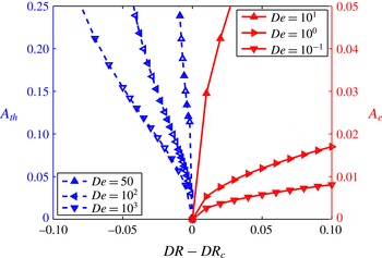
equal to zero in expression (2.26). Figure 11 plots the amplitude at the fixed point of the Landau equation, that is the equilibrium amplitude for
 $\mathit{De}<40$
(supercritical bifurcation) and the threshold amplitude for
 $\mathit{De}>40$
(subcritical bifurcation). In the latter regime, the threshold amplitude, which represents the amplitude of a disturbance that drives an instability even below the transition point, tends to decrease with further increase in the fluid elasticity. Thus, for highly elastic fluids, the spinning flow is highly susceptible to even a small-amplitude disturbance, which amplifies by nonlinear self-interaction and drives an instability.
The finite-amplitude manifold in the vicinity of the transition point. The role of the fluid elasticity is shown to be of dual nature. A supercritically stable branch is observed for
 $\mathit{De}<40$
and a subcritically unstable branch for
 $\mathit{De}>40$
. The XPP parameters are
 $r=2$
and
 $q=9$
.

To summarize the findings of the weakly nonlinear analysis, we show different regimes in the
 $\mathit{DR}$
–
 $\mathit{De}$
plane in figure 12. Here, the full line plots
 $\mathit{DR}_{c}$
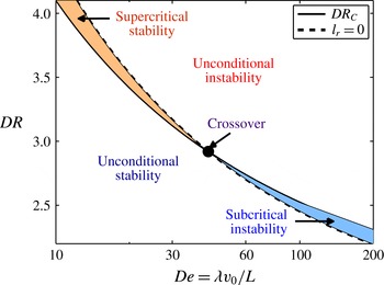
from the linear stability analysis. The region between the full line and the broken line on either side of the crossover point (
 $\mathit{De}\approx 40$
) indicates the supercritically stable and subcritically unstable regions. This broken line is, in fact, the locus of
 $l_{r}=0$
points at different Deborah numbers. For Deborah numbers below the crossover point (
 $\mathit{De}<40$
), the supercritical region indicates that the flow attains an oscillatory stationary state with sustained periodic oscillations along the fibre. For drawing with a draw ratio above the broken line, the flow becomes nonlinearly unstable, with high-amplitude oscillations, which may lead to breakage of the fibre when the cross-section area becomes very small. On the other side of the crossover point (
 $\mathit{De}>40$
), the spinning becomes unstable even for
 $\mathit{DR}<\mathit{DR}_{c}$
, provided that the disturbance amplitude is above a threshold value. As seen in figure 11, the subcritical branch tends to turn upward, which means that there exists a value of the draw ratio below which the flow remains stable irrespective of the disturbance amplitude. This value of
 $\mathit{DR}$
is indicated by the broken line in figure 12.
Neutral stability diagram in the
 $\mathit{DR}_{c}$
–
 $\mathit{De}$
plane indicating the regions of supercritically stable and subcritically unstable flow. Along the full line, the real part of the linear growth rate,
 $s_{r}$
, is zero. On the broken line, the real part of the Landau constant,
 $l_{r}$
, is zero. The two lines meet at the crossover point. The enclosed areas between the two lines before and after the crossover are the supercritical and subcritical Hopf bifurcation regions respectively. The XPP parameters are
 $r=2$
and
 $q=9$
.

Next, we examine the role of strain hardening in the finite-amplitude stability. In linear stability analysis, with an increase in the strain hardening parameter
 $q$
, the value of the critical draw ratio
 $\mathit{DR}_{c}$
shoots up significantly around
 $\mathit{De}\approx 0.1$
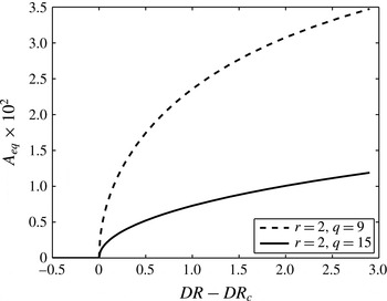
, as shown in figure 7(a). Thus, the stabilizing role of strain hardening in linear analysis has been established. Using weakly nonlinear analysis, we calculate the equilibrium amplitude
 $A_{e}$
for
 $\mathit{De}=0.11$
for two values of the parameter
 $q$
, as shown in figure 13. At this Deborah number, the bifurcation is supercritical and the equilibrium amplitude is found to decrease with increase in the strain hardening parameter
 $q$
. Thus, the stabilizing role of strain hardening is not only limited to linear analysis, but is also reflected in finite-amplitude analysis. Thus, the use of polymeric fluids with greater strain hardening effect leads to significant reduction in the extent of the draw resonance amplitude.
Variation in the equilibrium amplitude with the draw ratio (
 $\mathit{DR}-\mathit{DR}_{c}$
) for two values of the strain hardening parameter
 $q$
for
 $\mathit{De}=0.11$
. Increasing
 $q$
stabilizes the system and hence lowers the branch for
 $q=15$
as compared with
 $q=9$
, meaning a less pronounced draw resonance effect. The XPP parameter is
 $r=2$
.

While the linear stability analysis constructs a stability map in the
 $\mathit{DR}_{c}$
–
 $\mathit{De}$
plane, the weakly nonlinear analysis allows one to construct a curve for the variation in the equilibrium amplitude
 $A_{e}$
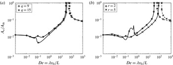
with the Deborah number. Figure 14 plots these curves for variation of the parameters in the XPP model. Here, the amplitude is calculated by using (2.26) in the vicinity of the critical point,
 $|\mathit{DR}-\mathit{DR}_{c}|/\mathit{DR}_{c}=1\,\%$
, where
 $\mathit{DR}_{c}$
is obtained from the neutral stability curves shown earlier in figure 7. The full line indicates a supercritical bifurcation and the broken line indicates a subcritical bifurcation. At the crossover point, the equilibrium amplitude diverges as the real part of the Landau constant,
 $l_{r}$
, goes through zero. The effect of the strain hardening parameter,
 $q$
, is shown in figure 14(a), where the equilibrium amplitude, indicative of the severity of the draw resonance in the supercritical region, is seen to be lower for a higher value of the parameter
 $q$
. The stabilizing role of strain hardening is also observed in the subcritical region, where the threshold amplitude for draw resonance onset is found to be higher for higher
 $q$
. In addition to reduction in
 $A_{e}$
in the supercritical regime, the enhancement in strain hardening also delays the crossover Deborah number for transition from supercritical stability to subcritical instability. We found that the crossover Deborah number shifts from
 $\mathit{De}\approx 40$
for
 $q=9$
to
 $\mathit{De}\approx 50$
for
 $q=15$
.
Variation of the equilibrium/threshold amplitude with
 $\mathit{De}$
. The draw ratio is fixed at 1 % deviation from the
 $\mathit{DR}_{c}$
value. The full line indicates the supercritically stable branch and the broken line represents the subcritically unstable branch. The divergence in amplitude occurs at the point of crossover from supercritical to subcritical bifurcation. (a) Effect of the strain hardening parameter,
 $q$
, for
 $r=2$
. (b) Effect of the ratio of relaxation times,
 $r$
, for
 $q=9$
.

The effect of another parameter in the XPP model,
 $r$
, the ratio of backbone orientation to stretch relaxation times, is depicted in figure 14(b). For
 $\mathit{De}>1$
, the stabilizing role of increasing
 $r$
, as indicated by a lower value of the equilibrium amplitude, is consistent with the similar stabilizing effect observed in linear stability analysis (refer to figure 7
b). Moreover, the crossover from supercritical to subcritical bifurcation is delayed from
 $\mathit{De}\approx 40$
for
 $r=2$
to
 $\mathit{De}\approx 105$
for
 $r=5$
. For
 $0.1<\mathit{De}<1$
, the equilibrium amplitude is significantly higher for higher values of
 $r$
, indicating intensified draw resonance due to strain softening caused by the orientation of the backbone chains.
5. Conclusion
We analyse the stability behaviour of the extensional flow of viscoelastic fluid that prevails during the isothermal fibre spinning process. The elongational flow in the air gap helps to orient polymeric chains along the flow direction, thus playing a major role in producing very thin fibres with high mechanical strength. The flow parameter in the process is termed the draw ratio,
 $\mathit{DR}$
, which governs the strength of the extension rate and is defined as the ratio of take-up to extrudate velocities. When the draw ratio exceeds a certain critical value,
 $\mathit{DR}_{c}$
, the profile of the fibre undergoes sustained periodic oscillations in the fibre cross-section area, a hydrodynamic instability known, in the literature, as draw resonance. With the objective of understanding the finite-amplitude stability behaviour of the spinning flow post-transition point, we first carry out a linear stability analysis. We restrict the analysis to only axisymmetric disturbances to the fibre cross-section area. The rheological description of the fluid, which consists of a melt of entangled polymers, is provided by the XPP model. The XPP model captures the extreme strain hardening effect under fast extensional flow observed in fibre spinning. For infinitesimal-amplitude disturbances, we estimate the critical draw ratio
 $\mathit{DR}_{c}$
as a function of the flow Deborah number.
It should be noted that the present analysis assumes the spinning flow to be isothermal. In practice, the hot spinline undergoes cooling by convection to the surrounding air as well as evaporative cooling (for solution spinning). Since the material rheology plays an important role in the stability behaviour, the enhancement in extensional viscosity due to the cooling effect would render stability to the spinning flow. However, for small-air-gap flow, the isothermal assumption would hold and the stabilizing role of non-isothermal effects might be negligible.
By using the theory of weakly nonlinear stability analysis, we study the role of finite-amplitude axisymmetric disturbances through nonlinearities present in the governing equations. In the neighbourhood of the transition point, the dynamics of the disturbance amplitude is governed by the Landau equation, which contains the higher-order correction to the linear growth rate, the Landau constant. For small values of the Deborah number (
 $\mathit{De}\lesssim 0.1$
), the real part of the Landau constant is found to be negative. Thus, the stabilizing effect of nonlinearities means that the initial small-amplitude disturbance grows to an equilibrium value, meaning that the bifurcation is supercritical. The equilibrium amplitude provides the amplitude of oscillations in the fibre cross-section area in the unstable region. As the fluid elasticity is increased, the equilibrium amplitude decreases until it reaches the lowest value at a Deborah number corresponding to the maximum strain hardening effect. Upon further increasing the Deborah number, the equilibrium amplitude increases, indicating the destabilizing role of nonlinearities. This behaviour is related to the strain softening effect in extensional viscosity for fast extensional flows.
At a certain Deborah number (
 $\mathit{De}\approx 40$
), the finite-amplitude branch shows a crossover from supercritical to subcritical bifurcation. In the subcritical case, the amplitude equation provides the threshold amplitude of disturbance to cause an instability in the linearly stable region. The area of subcritical instability increases with increasing extension rate, suggesting that the system continually grows susceptible to instability for even very-small-amplitude perturbations. Hence, practical operations are seldom feasible at such high extension rates.
Upon continuing the finite-amplitude branch in either the supercritical or subcritical regime, we also find a sign of upturn of the manifold. This allows us to predict the range of the draw ratio, around the critical value
 $\mathit{DR}_{c}$
, in which supercritically stable and subcritically unstable states can be realized. However, due to the validity of the weakly nonlinear analysis only in the proximity of the transition point, further higher-order effects, like turning of a manifold, should be confirmed from the full numerical simulation of spinning of viscoelastic fluid. The finite-amplitude stability behaviour of polymer fibre spinning presented here helps in tuning of the polymer rheology in order to either completely suppress or weaken the severity of draw resonance during the spinning process. The findings can also be viewed in the broader context of the stability behaviour of extensional flows of polymeric fluids.
Acknowledgements
One of the authors (P.C.) is deeply grateful to M. Bulters and R. Stepanyan at the Materials Sciences Center, DSM, The Netherlands for many prolonged and insightful discussions on polymer fibre spinning. The authors are grateful to the Department of Science and Technology, Government of India for financial support.
Supplementary data
Supplementary data is available at http://dx.doi.org/10.1017/jfm.2015.284.