2 Nonnegative solutions for realistic initial conditions

Model (1.1) is well-posed in the sense that every solution starting from a realistic (positive) initial condition remains nonnegative. In what follows we see (1.1) as a vector field defined on the set $\Omega :=\{(q,m,s)\in \mathbb {R}^3|\,\,q\geq 0, m\geq 0, s>0\}$ , and use the following standard notation [Reference Arnold2, Reference Dumortier, Llibre and Artés11] for its components:

$$ \begin{align*} X(q,m,s)=X_1(q,m,s)\dfrac{\partial}{\partial q}+X_2(q,m,s)\dfrac{\partial}{\partial m}+X_3(q,m,s)\dfrac{\partial}{\partial s}\,. \end{align*} $$

Let us study the behaviour of X in $\partial \Omega $ to show that $\Omega $ is invariant. Let us subdivide $\partial \Omega $ into the coordinate planes $\partial \Omega =\omega _{qm}\cup \omega _{qs}\cup \omega _{ms}$ , where $\omega _{qm}=\{(q,m,s)\in \mathbb {R}^3|\,\,q\kern1.4pt{\geq}\kern1.4pt 0, m\kern1.4pt{\geq}\kern1.4pt 0, s\kern1.4pt{=}\kern1.4pt0\}$ , $\omega _{qs}\kern1.4pt{=}\kern1.4pt\{(q,m,s)\kern1.4pt{\in}\kern1.4pt \mathbb {R}^3|\,\,q\kern1.4pt{\geq}\kern1.4pt 0, m\kern1.4pt{=}\kern1.4pt0, s\kern1.4pt{>}\kern1.4pt0\}$ , and $\omega _{ms}\kern1.4pt{=}\kern1.4pt\{(q,m,s)\kern1.4pt{\in} \mathbb {R}^3|\,\,q=0, m\geq 0, s>0\}$ .

The restriction of (1.1) to the plane $\omega _{qs}$ is

$$ \begin{align*} X(q,0,s)=(rs-\mu_1 q)\dfrac{\partial}{\partial q}+\alpha\dfrac{\partial}{\partial m}+{(\epsilon\alpha+\mu_3 s)\dfrac{\partial}{\partial s}}\,. \end{align*} $$

Since $\alpha>0$ , the vector field (1.1) on $\omega _{qs}$ points towards the interior of $\Omega $ . Similarly, the restriction of (1.1) to the plane $\omega _{ms}$ is

$$ \begin{align*} X(0,m,s)=r(m+s)\dfrac{\partial}{\partial q}+(\alpha-\mu_2 m)\dfrac{\partial}{\partial m}{+(\epsilon\alpha+\mu_3 s)\dfrac{\partial}{\partial s}}\,. \end{align*} $$

Since $r>0$ , it follows that the vector field X in $\omega _{ms}$ points towards the interior of $\Omega $ .

On the other hand, system (1.1) is not defined on the plane $\omega _{qm}$ . In order to analyse the behaviour of (1.1) near $\omega _{qm}$ , let us consider the time scaling $t\mapsto st$ . In this way, (1.1) becomes

(2.1) $$ \begin{align} X_0:\left\{\begin{aligned} \dot q &= r(m+s)s-\mu_1qs,\\ \dot m & = \dfrac{k_1qm^2}{1+\gamma m^2}+\alpha s-\mu_2ms, \\ \dot s & = k_2qm^2s+\epsilon\alpha s-\mu_3s^2. \end{aligned}\right. \end{align} $$

System (2.1) is topologically equivalent to (1.1) in $\Omega $ . Moreover, (2.1) is well defined for $s=0$ and, hence, it can be continually extended to the boundary plane $\omega _{qm}\subset \partial \Omega $ . The restriction of (2.1) to the plane $\omega _{qm}$ is

$$ \begin{align*} X_0(q,m,0)=\dfrac{k_1qm^2}{1+\gamma m^2}\dfrac{\partial}{\partial m}. \end{align*} $$

It follows that the (unique) solution of (2.1) with initial condition $(q(0),m(0), s(0))=(q_0,m_0,0)\in \omega _{qm}$ is given by

(2.2) $$ \begin{align} \left\{\begin{aligned} q(t) &= q_0,\\ m(t) & = \dfrac{-1+k_1q_0m_0t+\gamma m_0^2+\sqrt{4\gamma m_0^2+(k_1tq_0m_0+\gamma m_0^2-1)^2}}{2\gamma m_0},\\ s(t) & = 0. \end{aligned}\right. \end{align} $$

As a consequence, the set $\omega _{qm}$ is an invariant plane of (2.1) which consists of a continuum of straight lines parallel to the m-axis parameterized by (2.2). Moreover, both axes $q=0$ and $m=0$ consist of a continuum of equilibria.

Let us now study the behaviour of orbits of (2.1) near the invariant plane $\omega _{qm}$ . Let us search for the solution of (2.1) with initial condition $(q(0),m(0),s(0))=(q_0,m_0,\delta )\in \text {int}(\Omega )$ , with $0<\delta \ll 1$ sufficiently small. Specifically, consider a solution of the form:

(2.3) $$ \begin{align} \left\{\begin{aligned} q(t) &= q_0(t)+\delta q_1(t)+O(\delta^2),\\ m(t) & = m_0(t)+\delta m_1(t)+O(\delta^2),\\ s(t) & = s_0(t)+\delta s_1(t)+O(\delta^2), \end{aligned}\right. \end{align} $$

where $(q_0(t),m_0(t),s_0(t))$ is the solution of (2.1) in the limit as $\delta \rightarrow 0$ and, hence, it is given by (2.2). In this way, (2.3) is expressed as

(2.4) $$ \begin{align} \left\{\begin{aligned} q(t) &= q_0+\delta q_1(t)+O(\delta^2),\\ m(t) & = m_0(t)+\delta m_1(t)+O(\delta^2),\\ s(t) & = \delta s_1(t)+O(\delta^2), \end{aligned}\right. \end{align} $$

with

$$ \begin{align*}m_0(t)= \dfrac{-1+k_1q_0m_0t+\gamma m_0^2+\sqrt{4\gamma m_0^2+(k_1tq_0m_0+\gamma m_0^2-1)^2}}{2\gamma m_0}.\end{align*} $$

It follows that the higher-order terms of (2.4) must satisfy the initial conditions $(q_1(0),m_1(0),s_1(0))=(0,0,1)$ for $n=1$ , and $(q_n(0),m_n(0),s_n(0))=(0,0,0)$ for $n\geq 2$ . Substitution of (2.4) into (2.1) leads to the following differential equations for the $O(\delta $ ) terms of $q(t)$ :

$$ \begin{align*} \delta\dot{q}_1(t) = &\; r(m_0(t)+\delta m_1(t)+\cdots+\delta s_1(t)+\cdots)(\delta s_1(t)+\cdots)\\ &-\mu_1(q_0+\delta q_1(t)+\cdots)(\delta s_1(t)+\cdots) =\delta rm_0(t)s_1(t)-\delta\mu_1 q_0s_1(t)+O(\delta^2). \end{align*} $$

Hence,

(2.5a) $$ \begin{align} \dot{q}_1(t)=rm_0(t)s_1(t)-\delta\mu_1 q_0s_1(t), \hspace{5mm} q_1(0)=0. \end{align} $$

Similarly,

$$ \begin{align*}\dot m(t)=\dot{m}_0(t)+\delta\dot{m}_1(t) +O(\delta^2) = \dfrac{k_1q(t)m^2(t)}{1+\gamma m^2(t)}+\alpha s(t)-\mu_2 m(t)s(t).\end{align*} $$

For $0<\delta \ll 1$ sufficiently small we have

$$ \begin{align*} \dot{m}_0(t)+\delta\dot{m}_1(t) +O(\delta^2) =& \;\dfrac{k_1q_0m_0^2(t)}{1+\gamma m_0^2(t)} \nonumber \\ &+\delta\left( \dfrac{k_1q_1(t)m_0^2(t)}{1+\gamma m_0^2(t)}- \dfrac{2\gamma k_1q_0m_0^3(t)m_1(t)}{(1+\gamma m_0^2(t))^2}+ \dfrac{2k_1q_0m_0^2(t)m_1(t)}{1+\gamma m_0^2(t)}\right) \nonumber\\ & + \delta\alpha s_1(t)-\delta\mu_2 m_0(t)s_1(t)+O(\delta^2).\nonumber \end{align*} $$

Thus,

(2.5b) $$ \begin{align} \dot{m}_1(t)&=\dfrac{k_1q_1(t)m_0^2(t)}{1+\gamma m_0^2(t)}- \dfrac{2\gamma k_1q_0m_0^3(t)m_1(t)}{(1+\gamma m_0^2(t))^2}+ \dfrac{2k_1q_0m_0^2(t)m_1(t)}{1+\gamma m_0^2(t)}+ \alpha s_1(t)-\mu_2 m_0(t)s_1(t), \, \nonumber\\ m_1(0)&=0. \end{align} $$

Likewise,

$$ \begin{align*} \delta\dot{s}_1(t) =& \;k_2(q_0+\delta q_1(t)+\cdots)(m_0(t)+\delta m_1(t)+\cdots)^2(\delta s_1(t)+\cdots)+\epsilon\alpha(\delta s_1(t)+\cdots)\\ & - \mu_3(\delta s_1(t)+\cdots)^2 = \delta k_2 q_0m_0^2(t)s_1(t)+\delta\epsilon\alpha s_1(t)+O(\delta^2).\nonumber \end{align*} $$

Hence,

(2.5c) $$ \begin{align} \dot{s}_1(t)=(k_2 q_0m_0^2(t)+\epsilon\alpha)s_1(t), \quad s_1(0)=1. \end{align} $$

The initial value problem (2.5) defines any solution of (2.1) starting at a distance $0<\delta \ll 1$ from the invariant plane $\omega _{qm}$ with accuracy $O(1/\delta )$ . In particular, since $k_2 q_0m_0^2(t)+\epsilon \alpha>0$ , it follows from (2.5c) that $s_1(t)$ is an increasing function for every $t>0$ . Hence, the component $s(t)$ in (2.1) is increasing near the plane $s=0$ . Therefore, no trajectory of (2.1) with initial condition in $\text {int}(\Omega )$ can reach the boundary plane $\omega _{qm}$ in (finite or infinite) positive time.

Since (2.1) is topologically equivalent to (1.1) in $\Omega $ , we conclude from the analysis in this section that every trajectory of the original system (1.1) starting in $\Omega $ remains nonnegative.

3 Constant autoinducer concentration

To shed light on the understanding of QS we now analyse the bacteria interaction dynamics under the assumption of a constant autoinducer concentration $q_0> 0$ . In so doing, we have $\eta _1 = k_1q_0$ and $\eta _2 = k_2q_0$ as the motile and static bacteria response rates, respectively. From (1.1), upon substituting the rescaled variables for the bacteria population $u= (\eta _2/\eta _1)m$ and $ v= (\mu _3\eta _2/\eta _1^2)s$ as well as $\tau = \mu _3 t$ for time, and the new parameters

(3.1) $$ \begin{align} K = \gamma \bigg(\dfrac{\eta_1}{\eta_2}\bigg)^2\,, \quad b = \dfrac{\mu_2}{\mu_3}\,, \quad a= \dfrac{\eta_2 \alpha}{\eta_1 \mu_3}\,, \quad e = \dfrac{\mu_3 \varepsilon}{\eta_1},\, \end{align} $$

we obtain the following two-dimensional constant autoinducer system:

(3.2) $$ \begin{align} \begin{cases} \dot u =f(u,v), & f(u,v)=\dfrac{u^2}{v(1+Ku^2)}+a-bu, \\ \dot v = g(u,v), & g(u,v)=u^2+ae-v. \end{cases} \end{align} $$

Notice that key parameters arise so that:

1. (i) K plays a saturation role;

2. (ii) b characterizes the bacteria decay rate; and

3. (iii) a and e capture bacteria production-related roles as well as inversely and directly proportional dependence of the constant autoinducer concentration and decay rate variations, respectively. The latter shows that parameter product $ae$ only depends on the bacteria response to autoinducer capacities and production of static subpopulation.

3.1 Number of steady states

As the understanding of interactions between motile and static bacteria is the backbone of the communication mechanism via autoinducers, we examine the circumstances affecting the way subpopulations coexist or go extinct. Hence, we first look for positive steady states. Suppose that nullclines of (3.2) satisfy

(3.3a) $$ \begin{align} v &= \dfrac{u^2}{(1+Ku^2)(bu-a)}, \end{align} $$

(3.3b) $$ \begin{align} v &= u^2 +ae ,\qquad\ \qquad \end{align} $$

for $u,v>0$ . Notice that (3.3b) defines a convex parabola with vertex at $(0,ae)$ , and (3.3a) has an asymptote at $u = a /b $ . For values of $u< a/b$ , the corresponding v-values are negative, which is not biologically meaningful. Now, we find that the nullcline (3.3a) can be recast as a smooth function of u, which is positive and possesses critical points for $u>a/b$ as $v^\prime (u)=0$ is held. In so doing, we get that ${-2a+b(u-Ku^3)=0}$ must be satisfied. This yields, as a consequence of Descartes’ rule of signs, the existence of two positive roots such that $a/b<u_1^\star <u_2^\star $ as $a,b,K>0$ , where the lower value corresponds to a local minimum and the higher one to a local maximum. Thus, from both expressions in (3.3), we get that there are at most three positive steady states. This is schematically illustrated in Figure 1 for a system defined later in (3.5) which is equivalent to (3.2) in the interior of the first quadrant and is well defined along the axis $v=0$ . These sketches provide sensitive evidence that two saddle-node bifurcations may occur as two steady states are created by varying appropriate parameters (see panels (a) and (c), where the nullclines are tangent).

Figure 1

Nullcline sketches for key parameter values of e, where $b>K>a$ . Panels (a) and (c) show three steady states, two of which are positive (within first quadrant) and the third is the origin; in (b) three positive steady states are depicted; and (d) shows only one positive steady state. Panels (a) and (c) correspond to scenarios approximately at two saddle-node bifurcations. Here $\tilde {f}(u,v)=0$ and $\tilde {g}(u,v)=0$ stand for $\dot {u}=0$ and $\dot {v}=0$ in (3.5), respectively.

3.2 Local stability of positive steady states

We now pay attention to the local stability of positive steady states $(u_*,v_*)$ in (3.2). The Jacobian matrix of (3.2) at $(u_*,v_*)$ is

(3.4) $$ \begin{align} \mathbf{J} = \left(\begin{array}{@{}cc@{}} \dfrac{2u_*}{v_*(1+Ku_*^2)^2}-b & -\dfrac{u_*^2}{(1+Ku_*^2)v_*^2} \\[2ex] 2u_* & -1 \end{array} \right)\!, \end{align} $$

where, by setting $\mathcal {J}:=2u_*/[v_*(1+Ku_*^2)^2]$ , the trace is given by $\text {tra}(\mathbf {J}) = \mathcal {J}-b-1$ , and the determinant by $\text {det}(\mathbf {J}) = b-(1-u_*^2/[v_*(1+Ku_*^2)])\mathcal {J}$ . Notice that the entries $J_{12}$ , and $J_{22}$ of (3.4) are negative, while $J_{21}$ is positive. Hence, local stability features depend on whether the first entry $J_{11}= \mathcal {J}-b$ is greater or less than $1$ as follows from the Hartman–Grobman theorem [Reference Guckenheimer and Holmes17]. This is summarized as follows.

Proposition 3.1. Let $\mathcal {J}:=2u_*/[v_*(1+Ku_*^2)^2]$ . Then the local stability of a positive steady state $(u_*,v_*)$ of (3.2) is as follows.

1. (1) It is locally asymptotically stable if $\mathcal {J}< b+1$ and $b>(1-u_*^2/[v_*(1+Ku_*^2)])\mathcal {J}$ .

2. (2) It is a repeller if $\mathcal {J}> b+1$ and $b>(1-u_*^2/[v_*(1+Ku_*^2)])\mathcal {J}$ .

3. (3) It is a saddle point if $b<(1-u_*^2/[v_*(1+Ku_*^2)])\mathcal {J}$ .

We now analyse the dynamical behaviour in the neighbourhood of the origin.

3.3 Dynamics near the origin

Despite vector field (3.2) being defined on ${{\mathcal {D} = \{(u,v)\in \mathbb {R}^2 | \ u \geq 0, \, v>0 \}}}$ , a solution with $v=0$ corresponds to absence of static bacteria, which is a feasible biological scenario. In consequence, similarly to (2.1), we consider a map $t\mapsto t / v$ to get

(3.5) $$ \begin{align} Y_0:=\begin{cases} \dot{u} = \tilde{f}(u,v)\,, & \tilde{f}(u,v)=\dfrac{u^2}{1+Ku^2}+av-buv,\\ \dot{v} = \tilde{g}(u,v)\,, & \tilde{g}(u,v)=u^2v+aev-v^2, \end{cases} \end{align} $$

which is topologically equivalent to (3.2) and can be continually extended to the boundary axis $v=0$ .

Proposition 3.2. The origin of (3.5) is a repeller.

Proof. Since the eigenvalues of the Jacobian matrix at the origin are $\lambda _1=0$ and $\lambda _2=ae>0$ , with associated eigenvectors $v_1=(1,0)^t$ and $v_2=(1/e,1)^t$ , respectively, it follows that there exists a centre manifold

$$ \begin{align*}W^c=\{(u,v)\mid v=h(u):=a_2u^2+O(u^3),\ |u|<\delta\},\end{align*} $$

for $\delta>0$ sufficiently small [Reference Guckenheimer and Holmes17]. Since $W^c$ is invariant one must have

$$ \begin{align*}\tilde{g}(u,h(u))\equiv h'(u)\tilde{f}(u,h(u)),\end{align*} $$

for every $(u,v)\in W^c$ . It follows from this identity that $a_2=0$ and $h(u)=O(u^3)$ . Hence, the dynamics of (3.5) restricted to $W^c$ is equivalent to $\dot x=x^2+O(x^3).$ Therefore, the origin of (3.5) is a repeller.

4 Bifurcation analysis in the two-dimensional system

We now perform a numerical exploration with MatCont [Reference Govaerts, Kuznetsov, De Witte, Dhooge, Meijer, Mestrom, Riet and Sautois16] in order to identify the most relevant bifurcations when parameters e or b are varied slowly. Upon varying b, different bacteria decay rate scenarios are explored; meanwhile, variations of e reveal the impact of having several response rates as well as different production rates. We focus our analysis on the way bacteria decay rates coordinate the emergence of oscillations.

Figure 2 depicts bifurcation diagrams of system (3.2) for parameters e and b. In Figure 2(a), two saddle-node (SN) points are identified at $e_1$ and $e_2$ , where the system possesses only one unstable or stable steady state for $e<e_1$ and $e>e_2$ , respectively, and three coexisting equilibrium points for $e_1<e<e_2$ . Note that the case $e=e_1$ corresponds to the nullcline arrangement in Figure 1(a); the scenario with $e_1<e<e_2$ relates to Figure 1(b); the case $e=e_2$ corresponds to Figure 1(c); and $e>e_2$ is associated with Figure 1(d). On the other hand, in Figure 2(b), after setting $e=3$ , two SN points are shown at $b_1$ and $b_2$ in addition to a Hopf point (denoted by H, for simplicity) at $b_3$ . In both panels of Figure 2, the black curves represent asymptotically stable equilibria, the discontinuous branch between the two SN points is a saddle point, and the upper dashed curve is a repeller. This Hopf bifurcation is supercritical as the first numerically computed Lyapunov coefficient is negative. Hence, for $b_3<b<b_4$ a stable limit cycle arises and coexists with the stable equilibrium at the lower branch. This paves the way for the emergence of synchronizing dynamics under suitable initial conditions, as a result of the limit-cycle branch that originates from the H point and terminates at the lightly dashed saddle branch at $b_4$ , suggesting the potential occurrence of homoclinic orbits.

Figure 2

Bifurcation diagrams for bifurcation parameters e and b. Dashed and solid curves correspond to unstable and stable steady states, respectively, where heavily dashed branches gather repeller steady states while saddle steady states are collected by lightly dashed branches, and the solid grey branch consists of stable limit cycles. (a) With $b=1.4$ and $a=0.042$ fixed, we identify two saddle-node (SN) points located at $e_1\approx 1.948551$ and $e_2\approx 3.497398$ . (b) Upon fixing $e=3$ and $a=0.042$ , we find two SN points at $b_1\approx 1.128239$ and $b_2\approx 1.512641$ as well as a Hopf (H) point at $b_3\approx 1.168852$ which terminates at $b_4\approx 1.239672$ . Parameter value for $K=0.043$ .

A two-parameter continuation is conducted following Figure 2 to investigate how the bifurcations evolve with the simultaneous variation of both parameters. As parameters e and a are slowly varied from the SN points in Figure 2(a), a cusp point (CP) and a Bogdanov–Takens point (BT) are observed; see Figure 3. Additionally, the two-parameter continuation with respect to both b and e, starting from the H point, reveals a Bogdanov–Takens bifurcation as the organizing centre of the dynamics, as shown in Figure 4. Upon taking Proposition 3.2 into account, the parameter space of interest for b and e can be divided into the following regions:

Figure 3

Two-parameter continuation. The solid curve corresponds to the SN locus. A CP point is located at $(e,a)\approx (1.723644,0.123118)$ and a BT point at $(e,a)\approx (2.490826,0.066303)$ . Other parameter values: $b=1.4$ and $K=0.043$ .

Figure 4

Two-parameter continuation for parameters b and e. Four possible scenarios are categorized as follows. I: Stable steady state, where the population converges to a positive population density. IIa: Oscillation dynamics, where the bacteria approach a periodic solution. IIb: Oscillation dynamics and stable steady state (bistability), exhibiting oscillation dynamics and a stable node. The bold dashed curve captures homoclinic nonlinear transitions (hom). III: Stable steady state, where no periodic solutions arise as orbits asymptotically converge to a steady state. IV: Two stable steady states (bistability), where there are two stable steady states, a node and a focus, which are separated by a saddle point. The remaining parameters are set to $a=0.042$ and $K=0.043$ .

1. (I) Stable steady state. This region, though disconnected, exhibits a stable steady state, while the origin remains unstable. For values of b close to zero, the positive steady state is a stable node. As b increases slightly, this state transitions into a stable focus, driven by a shift from negative real eigenvalues to complex eigenvalues with negative real parts.

2. (II) Oscillation dynamics. The emergence of positive, stable periodic solutions plays a critical role in shaping the synchronized dynamical behaviour of bacterial populations. This phenomenon may stem from strong inter-bacterial communication. Notably, the lower SN dashed curve divides this region into two distinct subregions: in subregion (IIa), self-sustained oscillations dominate, whereas in subregion (IIb) (bistability), a stable steady state coexists with a limit cycle.

3. (III) Stable steady state. No limit cycle is observed on the right-hand bold dashed curve associated with the homoclinic bifurcation originating from the BT point.

4. (IV) Two stable steady states (bistability). This region contains three steady states: a stable node and a stable focus, separated by a saddle point. Consequently, the population converges to one of these two stable states depending on the initial conditions.

Notice that Figure 4 also shows that the larger the value of e, the smaller the range of values of b that can sustain oscillations. In other words, as e exceeds a certain value no synchronizing dynamics are possible, no matter the value of b. Parameter e plays a bacteria production role in the model. It is directly proportional to the rate of static bacteria production and inversely proportional to the constant autoinducer concentration. This could indicate that the oscillatory dynamics of the population is dependent on the interaction between the decay and production rates of the bacteria or the decay rates and the autoinducer concentration. The latter scenario will be explored in Section 5.

4.1 Hysteresis and synchronization

Now, as we have found such key dynamical events, which are characterized by parameters b and e, related to autoinducers concentration and bacterial decay rates, as can be seen in (3.1), we illustrate these transitions by considering a time-dependent variable $b=b(t)$ .

4.1.1 Linearly varying ${b}$

The model shows hysteresis as b is varied linearly back and forth. For instance, in Figure 5(a) we fix $e=1.0$ and continuously vary linearly from $b=1.0$ to $b=3.0$ . As can be seen, the solution decays in oscillatory fashion for values of b small enough (region I); then, as b crosses a corresponding Hopf bifurcation value, the solution amplitude starts increasing approaching a stable limit cycle (region II); then it finally approaches a stable steady state after the homoclinic bifurcation (regions III and I). In Figure 5(b), parameter b is traversed backwards, which yields a solution that remains in a stable node steady state throughout the first two regions it crosses (regions I and III). As it reaches the oscillation dynamics region, the solution spikes and approaches a limit cycle (subregions IIa, b). Finally, the solution begins to show a decaying amplitude oscillatory behaviour (region I).

Figure 5

A solution sample for time-dependent parameter b: (a) a solution with b linearly ranging from $b=1$ to $b=3$ with $e=1$ fixed; (b) a solution with parameter b going backwards from $b=3$ to $b=1$ with $e=1$ fixed; (c) parameter b linearly increases from $b=1.0$ to $b=1.5$ with $e=1.5$ fixed. Initial conditions are set to $(u,v)=(0.5,0.5)$ . Other parameter values: $a=0.042$ and $K=0.043$ .

Notice that in Figure 5(b), the solution’s behaviour is rather dissimilar to that when b increases (see Figure 5(a)), which indicates the existence of hysteretic-like features in the system as b is varied back and forth. In other words, the solutions depart from and return to the same initial state, exploring different dynamical regimes depending on the parameter pathways. These solutions exhibit both oscillatory and nonoscillatory behaviours with distinct characteristics, suggesting a robust feature of the system’s interaction. This resilience may be interpreted biologically as the bacteria population’s ability to preserve functionality despite external and internal perturbations, as highlighted in, for example, [Reference Kitano21]. Varying b from $b=1.0$ to $b=3.0$ and back illustrates how the dynamics of the solution changes for different bacteria decay rates for a constant value of e. When b values are close to $1$ , the decay rates of constant and static bacteria are similar. As b grows, the difference between the decay rates of the bacteria increases.

On the other hand, observe that in Figure 5(c), parameter $e=1.5$ is kept fixed and b varies from $b=1.0$ up to $b=1.5$ and remains at this value as the solution converges to a periodic solution (regions I and IIa). This periodic behaviour shows that the concentration of motile bacteria slightly rises before the static bacteria concentration and that its exponential decay is faster than that of the static population.

Figure 6

A sample solution for $e=1.0$ and b varying between $1$ and $3$ at different frequencies. Parameter $b(t)$ is depicted by the dotted curve for $A= 2$ , $B=1$ and $\varphi =3\pi /2$ . The solution is shown for three different frequency values as is shown in each panel. Other parameter values: $a=0.042$ and $K=0.043$ .

4.1.2 Periodically varying ${b}$

The bifurcation diagram in Figure 4 highlights the critical role of parameter b in the emergence of oscillatory behaviour, reflecting the impact of time-dependent variations in bacterial decay rates. We therefore proceed to illustrate crucial consequences as b varies periodically back and forth between $b=1.0$ and $b=3.0$ in a given period of time for a fixed e value. In doing so, we will gain insight into the effect of bacteria decay rates that vary in time. We consider an interval given by $t \, \in \, [0,2000]$ and a periodic decay rate parameter given by $b(t)=A+B\sin (\omega t + \varphi )$ , where A and B determine parameter bounds and $\omega $ and $\varphi $ are the frequency and phase at which b varies. Figure 6 shows three scenarios for b varying at different frequencies. These simulations suggest that, in order to observe meaningful dynamics, the value of $\omega $ must be small. For small $\omega $ , the solution will indeed show oscillations with a significantly small amplitude, but as the value of $\omega $ increases, the solution will behave as a constant state intermittently disrupted by spikes over time. In Figure 6 the solutions for $\omega = 0.010,\, 0.027$ and $0.044$ are depicted. For $\omega = 0.010$ , we see that as b starts to increase, the solution oscillates regularly. As $b(t)$ varies periodically the solutions alternate between periodic behaviour, oscillatory decay, and constant. That is, as b increases and the solution enters the oscillation region in Figure 4, the amplitude of the oscillations increases to remain constant. Notice that, as b starts to decrease, the solution becomes constant until it re-enters the oscillation region, when it spikes. This is characterized by the valley-like windows; see the upper panel. When $\omega =0.027$ and $0.044$ we see that, as parameter b takes decreasing values, the solution spikes as b enters the oscillation region. However, as $\omega $ increases, the stable spiral behaviour lasts less time, until it is no longer present in the solution. These sudden spikes in the solution indicate excitatory dynamics in the system. The previous results convey that the dynamics of the two-dimensional system (3.5) is sensitive to fast varying parameter b, which suggests that the time scale at which the bacteria decay rates change has a rather direct impact on the possible emergence of synchronization dynamics.

4.2 Andronov–Hopf bifurcation in the two-dimensional system

We now proceed to compute the normal forms for the Hopf bifurcation as is crucial for the dynamical shaping for the distinguished parameter values of Table 1.

Table 1

Parameter values used in Section 4.

Let $(U,V)\in \mathbb {R}^2_+$ be the positive coordinates of an equilibrium of (3.2) in the first quadrant. Then the set of equations $f(U,V)=0$ and $g(U,V)=0$ define implicitly a locally invertible transformation given by $\Psi :\Lambda \longrightarrow \mathbb {R}^4_+$ ,

(4.1) $$ \begin{align} (U,V,b,K)\mapsto(a,e,b,K):=&\left(\dfrac{U (b (1 + K U^2) V-U)}{V + K U^2 V}, \dfrac{(V-U^2) (V + K U^2 V)}{U (b (1 + K U^2) V-U)}, b,K\right), \end{align} $$

in $\Lambda :=\{(U,V,b,K)\in \mathbb {R}^4_+\, \mid b (1 + K U^2) V-U>0,\, V-U^2>0\}.$ Then the vector field (3.2) in parameter space $\Lambda $ has the form

(4.2) $$ \begin{align} \left\{ \begin{aligned} x' &= \dfrac{x^2}{y + K x^2 y} + \dfrac{U (b (1 + K U^2) V-U)}{V + K U^2 V} - b x \,, \\ y' &= x^2 + V -U^2 - y\,, \end{aligned} \right. \end{align} $$

where, for convenience, we use the notation $(x,y)$ to designate the state variables, and we denote $x'=dx/dt$ , $y'=dx/dt$ . System (4.2) is $C^{\infty }$ -equivalent to (3.2) in parameter space $\Lambda $ . Moreover, the (positive) equilibrium coordinates appear now as the explicit parameters $(U,V)$ . In what follows in this section, we will give conditions such that (4.2) undergoes a generic Hopf bifurcation at $(U,V)$ (see [Reference Guckenheimer and Holmes17, Reference Kuznetsov23] for more details).

The Jacobian matrix of (4.2) at $(U,V)$ is

(4.3) $$ \begin{align}J(U,V)=\begin{pmatrix} -b+\dfrac{2 U}{(1 + K U^2)^2 V} & \dfrac{-U^2}{(1 + K U^2) V^2} \\[2ex] 2U & -1 \end{pmatrix}. \end{align} $$

The trace T and determinant D of $J(U,V)$ are given by

$$ \begin{align*} T&=T(U,V,b,K)=-1 -b+\dfrac{2 U}{(1 + K U^2)^2 V},\quad D=\det[J(U,V)]= (V + K U^2 V)^{-2} \hat{D} \end{align*} $$

where

$$ \begin{align*} \hat{D}=\hat{D}(U,V,b,K)=2 U^3 + 2 K U^5 - 2 UV + b V^2 + 2 b K U^2 V^2 + b K^2 U^4 V^2. \end{align*} $$

Whenever $T=0$ and $D>0$ , the eigenvalues of $J(U,V)$ are purely imaginary and nontrivial. Moreover, since we have partial derivative $T_b(U,V,b,K)=-1<0,$ the Hopf bifurcation in (4.2) is generically unfolded by parameter b. In particular, it follows from there that the equation $T(U,V,b,K)=0$ implicitly defines the function

$$ \begin{align*} b(U,V,K)=-1 +\dfrac{2 U}{(1 + K U^2)^2 V}.\end{align*} $$

We now calculate the first Lyapunov quantity [Reference Guckenheimer and Holmes17, Reference Kuznetsov23] in order to determine genericity conditions. We follow the derivation in [Reference Guckenheimer and Holmes17] and move the equilibrium $(U,V)$ of the system (4.2) to the origin via the translation $x\mapsto x+U$ , $y\mapsto y+V$ to obtain the equivalent system

(4.4) $$ \begin{align} \left\{ \begin{aligned} x' &= U \left(\dfrac{b - U}{V + K U^2 V}\right) - b (U + x) + \dfrac{(U + x)^2}{V + y + K (U + x)^2 (V + y)}, \\ y' &= 2 U x + x^2 - y\,. \end{aligned} \right. \end{align} $$

In particular, the Jacobian matrix of (4.4) at the equilibrium $(0,0)$ coincides with $J(U,V)$ in (4.3). Upon substituting the function $b(U,V,K)$ into $J(U,V)$ , we get

$$ \begin{align*}J_H(U,V)=\begin{pmatrix} 1 & \dfrac{-U^2}{(1 + K U^2) V^2} \\[2ex] 2U & -1 \end{pmatrix}, \end{align*} $$

with $T_H\kern1.5pt{:=}\kern1.5pt\textrm {tra}\,[J_H(U,V)]\equiv 0$ and $\det [J_H(U,V)]\kern1.5pt{=}\kern1.5pt D_H\kern1.5pt{:=}\kern1.5pt D|_{T=0}\kern1.5pt{=}\kern1.5pt (2 U^3 - V^2 - K U^2 V^2)/ {(1 + K U^2) V^2}.$

If $D_H>0$ , then $\mathbf {v}_1=({1}/{2U},1)^t$ and $\mathbf {v}_2=(-{w}/{2U}, 0)^t$ are the generalized eigenvectors of $J_H(U,V)$ , where $w=\sqrt {D_H}$ . The change of coordinates $(x,y)^t\mapsto [\mathbf {v}_{1} \, \mathbf {v}_{2}] (x, y)^t $ , where t stands for transpose, allows us to express system (4.4) with $T_H=0$ in the form

(4.5) $$ \begin{align} \left(\begin{array}{@{}c@{}} x'\\ y' \end{array} \right)=\left( \begin{array}{@{}cc@{}} 0 & -w\\ w & 0 \end{array} \right)\left(\begin{array}{@{}c@{}} x \\ y \end{array} \right)+\left(\begin{array}{@{}c@{}} P(x,y) \\ Q(x,y) \end{array} \right), \end{align} $$

where

(4.6a) $$ \begin{align} P(x,y)=\dfrac{1}{4 U^2}x^2 - \dfrac{w }{2 U^2} x y+ \dfrac{w^2 }{4 U^2}y^2 \end{align} $$

and

$$ \begin{align*} &Q(x,y)\\&\quad= \dfrac{-16 K U^7 - 8 K^2 U^9 - 2 U V^2 + V^3 + 3 K U^2 V^3 + 3 K^2 U^4 V^3}{4 U^2 (V + K U^2 V)^3 w}x^2\nonumber\\ &\qquad + \dfrac{ K^3 U^6 V^3 + 8 U^5 (-1 + K V) + 2 U^3 V (4 + 3 K V)}{4 U^2 (V + K U^2 V)^3 w}x^2\nonumber\\ &\qquad +\dfrac{-4 K U^5 + 2 U V - V^2 - 3 K U^2 V^2 - 3 K^2 U^4 V^2 - K^3 U^6 V^2 - U^3 (4 + 6 K V)}{2 U^2 (1 + K U^2)^3 V^2}xy\nonumber\\ &\qquad +\dfrac{(-2 U + 6 K U^3 + V + 3 K U^2 V + 3 K^2 U^4 V + K^3 U^6 V) w}{4 U^2 (1 + K U^2)^3 V}y^2\nonumber\\ &\qquad + \dfrac{ 12 K^2 U^8 + 4 K^3 U^{10} - 4 K U^6 (-3 + K V) + V^2 (1 + 2 K V)}{2U (V + K U^2 V)^4 w}x^3\nonumber\\ &\qquad + \dfrac{U^4 (4 - 8 K V - 3 K^2 V^2) - 2 U^2 V (2 + K V + K^2 V^2)}{2U (V + K U^2 V)^4 w}x^3\nonumber\\ &\qquad + \dfrac{4 K^2 U^6 - 2 V (1 + 3 K V) + 2 K U^4 (4 + 3 K V) + U^2 (4 + 4 K V + 6 K^2 V^2)}{2U (1 + K U^2)^4 V^3}x^2y\nonumber\\ &\qquad +\dfrac{(1 - 2 K (U^2 - 3 V) - 3 K^2 (U^4 + 2 U^2 V)) w}{2U (1 + K U^2)^4 V^2}xy^2+\dfrac{ K (-1 + K U^2) w^2}{U (1 + K U^2)^4 V}y^3\\ &\qquad +O(||(x,y)||^4),\nonumber \end{align*} $$

in a Taylor expansion near $(x,y)=(0,0).$

System (4.5), equations (4.6) and $w=\sqrt {D_H}$ allow us to use the derivation in [Reference Guckenheimer and Holmes17] for the direct calculation of the first Lyapunov quantity $L_1$ . In so doing, we obtain the expression

$$ \begin{align*}L_1=\dfrac{ 1}{64 w^2 (1 + K U^2)^6 U^4V^5 }\,l_1,\end{align*} $$

where

$$ \begin{align*} l_{1}&=-32 K^3 U^{14} + 16 K^4 U^{13} V^2 w^2 + 2 U^2 V^3 (2 + 3 K V^2 (w-1) w) (1 + w^2) \\ &\quad- 2 U V^4 (1 + w^2)^2 + V^5 w ( -1+w - w^2 + w^3) \\ & \quad- 4 U^3 V^3 (-1 + (1 + 6 K V) w^2 + 6 K V w^4)+ 4 K^3 U^{11} V^2 (16 w^2 + K (V + 7 V w^2)) \\ &\quad+ U^4 V^2 (-24 K V (1 + w^2) - 8 (3 + w^2) + 15 K^2 V^3 w (-1 + w - w^2 + w^3)) \\ &\quad+ 4 U^6 V (12 + 9 K^2 V^2 (1 + w^2) + 4 K V (3 + w^2) + 5 K^3 V^4 w (-1 + w - w^2 + w^3)) \\ &\quad+ K^2 U^{12} (-96 - 48 K V + K^4 V^5 w (-1 + w - w^2 + w^3))\\ & \quad+ 6 K U^{10} (-16 - 8 K V + K^4 V^5 w (-1 + w - w^2 + w^3))\\ &\quad + U^8 (-32 + 48 K V + 24 K^2 V^2 (3 + w^2)+ 15 K^4 V^5 w (-1 + w - w^2 + w^3)) \\ & \quad - 4 U^5 V^2 (-4 w^2 - 4 K V (1 + w^2) + 3 K^2 V^2 (-1 + w^4)) \\ & \quad+ 2 K^2 U^9 V^2 (48 w^2 + 8 K (V + 5 V w^2) + 3 K^2 V^2 (1 + 6 w^2 + 5 w^4))\\ & \quad + 8 K U^7 V^2 (8 w^2 + 3 K (V + 3 V w^2) + K^2 V^2 (2 + 7 w^2 + 5 w^4)). \end{align*} $$

Thus, we have obtained the following result.

Theorem 4.1. Let $(U,V,b,K)\in \Lambda $ be such that $T_H=0$ , $D_H>0$ and $l_1\neq 0$ . Then (4.2) undergoes a codimension- $1$ Hopf bifurcation at the equilibrium $(U,V)$ . In particular, if $l_1<0$ (respectively, $l_1>0$ ), the Hopf bifurcation is supercritical (respectively, subcritical), and a stable (respectively, unstable) limit cycle bifurcates from $(U,V)$ under suitable parameter variation.

Whenever condition $l_1\neq 0$ in Theorem 4.1 does not hold, the Hopf bifurcation of (4.2) at $(U,V)$ is degenerate. The actual codimension of this singularity—and the stability of further limit cycles that bifurcate—is determined by the sign of the so-called second Lyapunov quantity $L_2$ (see, for instance, [Reference Kuznetsov23]). However, since the transformation (4.1) is invertible in the parameter set $\Lambda $ , numerical evidence suggests that $l_1<0$ for representative parameter values in Table 1 and, hence, the bifurcating limit cycle is stable. Furthermore, bifurcation theory ensures that the existence and stability of this stable periodic orbit persist for an open set of parameter values in the region $T(U,V,b,K)>0$ , that is, when the focus at $(U,V)$ is unstable [Reference Guckenheimer and Holmes17, Reference Kuznetsov23].

4.3 Bogdanov–Takens bifurcation in the two-dimensional system

We now give conditions such that our model undergoes a Bogdanov–Takens bifurcation under suitable parameter variation at a positive equilibrium. We prove the existence of a germ of a BT bifurcation and show that our system (under certain conditions) is locally topologically equivalent to a normal form of the BT bifurcation. We refer to [Reference Kuznetsov23] and the references therein for the derivation of the genericity and transversality conditions that need to be verified during this proof.

For the sake of clarity, it is convenient to state the dependence of the vector field (3.2) on parameters b and K explicitly. Hence, throughout this section we denote ${X: \mathbb {R}^4_+\longrightarrow \mathbb {R}^2_+}$ ,

$$ \begin{align*} X(x,y;b,K) = \left( \dfrac{x^2}{(1 + K x^2)y} + \alpha - b x, x^2 + \alpha\epsilon - y \right), \end{align*} $$

where we use notation $(x,y)$ for the state variables. Also, let us denote the Jacobian matrix of X with respect to the variables $(x,y)$ by

$$ \begin{align*}\dfrac{\partial X}{\partial(x,y)}(x,y;b,K)=\left( \begin{array}{@{}cc@{}} -\dfrac{-2 x + b y + 2 b K x^2 y + b K^2 x^4 y}{(1 + K x^2)^2 y} & -\dfrac{x^2}{(1 + K x^2) y^2} \\[2ex] 2x & -1 \\ \end{array} \right).\end{align*} $$

Step 1. We verify that the system may exhibit a singularity with a double zero eigenvalue and geometric multiplicity $1$ .

Lemma 4.2. Consider the set

$$ \begin{align*} \Omega_{BT}&=\{(x,y)\in\mathbb{R}^2_+\, | \, -2 x^5 + y^3>0, 2 x^3 - y^2>0, \ -2 x^5 + y^3- x^3 y >0, \\ &\qquad (x^2 - y)(2 x^5 + x^3 y - y^3)>0, \ 4 x^5 - x^3 y - 6 x^2 y^2 + 4 y^3\neq0\}. \end{align*} $$

Then there is a positive equilibrium $(U,V)\in \Omega _{BT}$ of (3.2) and there are positive parameter values

$$ \begin{align*}(b^*,K^*)=\bigg(\dfrac{-2 U^5 + V^3}{2 U^5},\dfrac{2 U^3 - V^2}{U^2 V^2}\bigg)\in\mathbb{R}^2_+ \quad \text{such that}\ \dfrac{\partial X}{\partial(x,y)}\bigg|_{(U,V;b^*,K^*)}\end{align*} $$

is nilpotent.

Proof. In order to prove this lemma, we look for solutions $(x,y,b,K)$ of the algebraic system

(4.7a) $$ \begin{align} \dfrac{x^2}{(1 + K x^2)y} + \alpha - b x&=0 ,\ \end{align} $$

(4.7b) $$ \begin{align} \qquad\quad\kern1.3pt x^2 + \alpha\varepsilon - y &=0, \end{align} $$

(4.7c) $$ \begin{align} \textrm{tra}\,\bigg[\dfrac{\partial X}{\partial(x,y)}(x,y;b,K)\bigg]&=0,\quad \end{align} $$

(4.7d) $$ \begin{align} \det \bigg[\dfrac{\partial X}{\partial(x,y)}(x,y;b,K)\bigg]&=0,\quad \end{align} $$

with $(x,y)\in \Omega _{BT}$ , $b>0$ and $K>0$ . Solving for b and K in (4.7c)–(4.7d) leads to

$$ \begin{align*}b=\dfrac{-2 x^5 + y^3}{2 x^5}>0\quad \text{and} \quad K=\dfrac{2 x^3 - y^2}{x^2 y^2}>0.\end{align*} $$

Substitution of $(b,K)$ in (4.7a)–(4.7b) and solving for $(\alpha ,\varepsilon )$ leads to

(4.8) $$ \begin{align} \alpha=\dfrac{-2 x^5 + y^3- x^3 y }{2 x^4} \quad \text{and} \quad \varepsilon =\dfrac{2 x^4 (x^2 - y)}{2 x^5 + x^3 y - y^3}\,. \end{align} $$

In particular, notice that $\alpha>0$ and $\varepsilon>0$ , since $(x,y)\in \Omega _{BT}.$ The map $(x,y)\mapsto (\alpha ,\varepsilon )$ defined by (4.8) has a Jacobian matrix given by

$$ \begin{align*} \dfrac{\partial(\alpha,\varepsilon)}{\partial(x,y)}=\left( \begin{array}{@{}cc@{}} -1 + \dfrac{y}{2 x^2} - \dfrac{2 y^3}{x^5} & -\dfrac{x^3 - 3 y^2}{2 x^4} \\[2ex] \dfrac{2 x^3 (2 x^7 + 5 x^5 y - x^3 y^2 - 6 x^2 y^3 + 4 y^4)}{(2 x^5 + x^3 y - y^3)^2} & \dfrac{-6 x^9 + 6 x^6 y^2 - 4 x^4 y^3}{(2 x^5 + x^3 y - y^3)^2} \end{array} \right)\,, \end{align*} $$

which has the determinant

$$ \begin{align*}\det \bigg[\dfrac{\partial(\alpha,\varepsilon)}{\partial(x,y)}\bigg]=\dfrac{4 x^5 - x^3 y - 6 x^2 y^2 + 4 y^3}{x(2 x^5 + x^3 y - y^3)}.\end{align*} $$

Therefore, since $\det [ {\partial (\alpha ,\varepsilon )}/{\partial (x,y)}]\neq 0$ , the inverse function theorem ensures that system (4.8) is locally invertible. Then the solution of (4.7) is given by $(x,y,b,K)=(U,V,b^*,K^*)\in \mathbb {R}^4_+$ , where $(U,V)$ is locally defined by the inverse map of (4.8), and

$$ \begin{align*}b^*=\dfrac{-2 U^5 + V^3}{2 U^5}, \quad K^*=\dfrac{2 U^3 - V^2}{U^2 V^2}.\end{align*} $$

Hence, at $(b,K)=(b^*,K^*)$ the equilibrium $(U,V)$ of the system (3.2) has a Jacobian matrix given by

(4.9) $$ \begin{align} \dfrac{\partial {X}}{\partial(x,y)}(U,V;b^*,K^*)=\left( \begin{array}{@{}cc@{}} 1 & -\dfrac{1}{2U} \\[2ex] 2U & -1 \\ \end{array} \right) \end{align} $$

with a double zero eigenvalue. In particular, note that (4.9) is not the null matrix. The corresponding generalized eigenvectors of (4.9) are given by

(4.10) $$ \begin{align} \mathbf{v}_1=\bigg(\dfrac{1}{2U},1\bigg)^t \quad \text{and} \quad \mathbf{v}_2=(1,-1 + 2 U)^t\,. \end{align} $$

It follows that (4.9) is nilpotent and that the double zero eigenvalue has geometric multiplicity $1$ . This completes the proof.

Step 2. We now state the following transversality condition of a Bogdanov–Takens bifurcation.

Lemma 4.3. Let $(U,V,b^*,K^*)$ be as in Lemma 4.2 and consider the map $ {\Psi :\mathbb {R}^4\rightarrow \mathbb {R}^4}$ ,

$$ \begin{align*} (x,y,b,K)\mapsto\left(\dfrac{x^2}{(1 + K x^2)y} + \alpha - b x, x^2 + \alpha\epsilon - y ,T,D\right), \end{align*} $$

where T and D are the trace and determinant of the matrix $({\partial X})/({\partial (x,y)})(x,y;b,K),$ respectively. Then the map $\Psi $ is regular at $(x,y,b,K)=(U,V,b^{\ast },K^{\ast })$ .

Proof. The $4\times 4$ Jacobian matrix $D\Psi =D\Psi (x,y;b,K)$ of the map $\Psi $ is

$$ \begin{align*} D\Psi= \left( \begin{array}{@{}ccrc@{}} -b - \dfrac{2 K x^3}{(1 + K x^2)^2 y} + \dfrac{2 x}{(1 + K x^2) y} & \dfrac{-x^2}{(1 + K x^2) y^2} & -x & \dfrac{-x^4}{(1 + K x^2)^2 y^2} \\[2ex] 2x & -1 & 0& 0\\[2ex] \dfrac{2 - 6 K x^2}{(1 + K x^2)^3 y} & \dfrac{-2 x}{(y + K x^2 y)^2} & -1 & \dfrac{-4 x^3}{(1 + K x^2)^3 y} \\[2ex] \dfrac{8 K x^4 + 2 K^2 x^6 - 2 y + 6 x^2 (1 + K y)}{(1 + K x^2)^3 y^2} & \dfrac{-4 x^3 - 4 K x^5 + 2 x y}{(1 + K x^2)^2 y^3} & 1 & \dfrac{-2 (x^5 + K x^7 - 2 x^3 y)}{(1 + K x^2)^3 y^2} \end{array} \right). \end{align*} $$

After some calculations, we have

$$ \begin{align*}\det [D\Psi(x,y,b,K)]=\dfrac{2x^5}{(y + K x^2 y)^4}F(x,y,b,K)\end{align*} $$

 with

$$ \begin{align*} F(x,y,b,K)=-2 K x^5 - 9 x y + b y^2 + 2 b K x^2 y^2 + b K^2 x^4 y^2 + x^3 (10 + K y). \end{align*} $$

In particular, straightforward substitution and algebraic simplification leads to

$$ \begin{align*} F(U,V,b^{\ast},K^{\ast})=-\dfrac{2U}{V^2}(4 U^5 - U^3 V - 6 U^2 V^2 + 4 V^3)\neq0\,, \end{align*} $$

since $(U,V)\in \Omega _{BT}$ . It follows that $ \det [D\Psi (U,V,b^{\ast },K^{\ast })]\neq 0, $ which ensures that the map $\Psi $ is regular at $(x,y,C,Q)=(U,V,b^{\ast },K^{\ast })$ .

Step 3. We now construct a change of coordinates to transform $X(x,y;b,K)$ into a normal form of the Bogdanov–Takens bifurcation; we refer to [Reference Kuznetsov23] once again.

Lemma 4.4. Let $(U,V,b^*,K^*)$ be as in Lemma 4.2 and consider the following auxiliary expressions:

$$ \begin{align*} G_1=8 U^{10} - 2 U^8 V - 4 U^5 V^3 - 3 U^3 V^4 + 2 V^6\,, \quad G_2=2 U^5 + 3 U^3 V - 2 V^3\,. \end{align*} $$

If $G_1\neq 0$ and $G_2\neq 0$ , then there exists a smooth, invertible transformation of coordinates, an orientation-preserving time rescaling, and a reparametrization such that, in a sufficiently small neighbourhood of $(x,y,b,K)=(U,V,b^{\ast },K^{\ast })$ , system (3.2) is topologically equivalent to a normal form of the codimension- $2$ Bogdanov–Takens bifurcation.

Proof. Let us set up the equilibrium $(U,V)\in \Omega _{BT}$ of (3.2) to the origin via the translation $x\mapsto x+U$ , $y\mapsto y+V$ to obtain the equivalent system

(4.11) $$ \begin{align} Y:\left\{ \begin{aligned} x' &= \alpha + (x + U)\left( -b+\dfrac{(x + U)}{(1 + K (x + U)^2) (y + U)}\right), \\ y' &= \alpha\varepsilon + (x + U)^2 - y - V\,. \end{aligned} \right. \end{align} $$

In particular, the Jacobian matrix of (4.11) at the equilibrium $(0,0)$ at the bifurcation point $(b^*,K^*)$ coincides with $({\partial {X}})/({\partial (x,y)})(U,V;b^*,K^*)$ in (4.9).

Let $\mathbf {P}=[\mathbf {v}_1, \mathbf {v}_2]$ be the matrix whose columns are $\mathbf {v}_1$ and $\mathbf {v}_2$ ; see (4.10). Next, consider the following change of coordinates:

$$ \begin{align*} \left( \begin{array}{@{}c@{}} u\\ v \\ \end{array} \right) = \mathbf{P}^{-1}\left( \begin{array}{@{}c@{}} x\\ y \\ \end{array} \right). \end{align*} $$

Then the vector field given by

$$ \begin{align*} \mathbf{J}=\mathbf{P}^{-1}\circ Y\circ\mathbf{P} \end{align*} $$

is $\mathcal {C}^{\infty }$ -conjugated to Y in (4.11).

Taking a Taylor expansion of $\mathbf {J}(u,v;b,K)$ with respect to $(u,v)$ around $(u,v)=(0,0)$ and evaluating at $(b,K)=(b^{\ast },K^{\ast })$ , we obtain

$$ \begin{align*} \left( \begin{array}{@{}c@{}} \dot{u}\\ \dot{v} \\ \end{array} \right) = \left( \begin{array}{@{}cc@{}} 0 & 1 \\ 0 & 0 \\ \end{array} \right) \left( \begin{array}{@{}c@{}} u\\ v \\ \end{array} \right)+ \dfrac{1}{2} \left( \begin{array}{@{}c@{}} a_{20}u^2+2\,a_{11}uv+a_{02}v^2+O(||(u,v)||^3)\\ b_{20}u^2+2\,b_{11}uv+b_{02}v^2+O(||(u,v)||^3)\\ \end{array} \right), \end{align*} $$

where we have

$$ \begin{align*} a_{20}&=\dfrac{1}{4U^{10} V}( 8 U^{10} - 16 U^{11} + 4 U^9 V - 4 U^5 V^3 + 8 U^6 V^3- 3 U^3 V^4 + 6 U^4 V^4 .\\ &+ 2 V^6 - 4 U V^6),\\ b_{20}&=\dfrac{1}{4 U^{10} V}(8 U^{10} - 2 U^8 V - 4 U^5 V^3 - 3 U^3 V^4 + 2 V^6),\\ b_{11}&= \dfrac{1}{2 U^9 V}(-4 U^9 + 8 U^{10} - 2 U^8 V + U^4 V^3) - \dfrac{1}{2 U^9 V}(4 U^5 V^3 + 3 U^3 V^4 - 2 V^6). \end{align*} $$

If $b_{20}\neq 0$ and $a_{20}+b_{11}\neq 0$ , then the theory of normal forms for bifurcations [Reference Kuznetsov23] ensures that our system fulfils the necessary genericity conditions to undergo a codimension- $2$ Bogdanov–Takens bifurcation. In particular, condition $G_1\neq 0$ ensures that $b_{20}\neq 0$ . Furthermore, after some algebraic manipulation one obtains $ a_{20}+b_{11}= -V^2G_2/4U^{10}$ .

In summary, Lemmas 4.2 and 4.3, and inequality $G_1G_2\neq 0$ ensure that the genericity and transversality conditions of a codimension- $2$ Bogdanov–Takens normal form are satisfied. Hence there exist a smooth, invertible transformation of coordinates, an orientation-preserving time rescaling, and a reparameterization such that, in a sufficiently small neighbourhood of $(x,y,\alpha ,k)=(U,V,b^{\ast },K^{\ast })$ , system (3.2) is topologically equivalent to one of the following normal forms of a Bogdanov–Takens bifurcation (see, for instance, [Reference Kuznetsov23]):

(4.12) $$ \begin{align} \left\{ \begin{aligned} \dot{\xi}_1 & = \xi_2\,, \\ \dot{\xi}_2 & = \beta_1+\beta_2 \xi_2 +\xi_2^2\pm \xi_1\xi_2\,,\\ \end{aligned} \right. \end{align} $$

where the sign of the term $\xi _1\xi _2$ in (4.12) is determined by the sign of $(a_{20}+b_{11})b_{20}$ .

The next theorem is a straightforward consequence from the findings in Lemmas 4.2, 4.3 and 4.4, as can be seen in [Reference Guckenheimer and Holmes17, Reference Kuznetsov23], and it summarizes the main result in this section.

Theorem 4.5. Let $(U,V,b^*,K^*)$ be as in Lemma 4.2 and consider the quantities $G_1$ and $G_2$ defined in Lemma 4.4. Then if $(b,K)=(b^*,K^*)$ , system (3.2) undergoes a codimension- $2$ Bogdanov–Takens bifurcation at $(x,y)=(U,V).$

5 Bifurcation and chaos in the three-dimensional system

As seen from the rescaled parameters in (3.1), parameters e, b and a capture the bacterial population’s response to autoinducers at constant concentration, as well as the decay rates of both bacterial subpopulations. Based on this, we analyse the effects of slowly varying the static bacteria’s response to autoinducer presence and motile bacteria’s saturation parameter, while the autoinducer concentration changes according to its dynamic production. Thus, to understand the emerging global behaviour, we perform a bifurcation analysis of system (2.1) using Auto [Reference Doedel, Champneys, Dercole, Fairgrieve, Kuznetsov, Oldeman, Paffenroth, Sandstede, Wang and Zhang9], allowing both parameters $k_2$ and $\gamma $ to vary slowly. The other parameters remain fixed in their typical values as in Table 2, except for $\mu _1=0.2$ and $\mu _2=0.7$ . Figure 7 shows the bifurcation diagram in the $(k_2,\gamma )$ plane. There curves of saddle-node (LP) and supercritical Hopf (labelled HB in this section) bifurcation meet at a BT point. Also, a curve of Shilnikov homoclinic bifurcation (hom) emerges from the point BT. A codimension- $2$ Belyakov point ( $B_c$ ) on the curve hom marks the onset of chaotic dynamics. To the right of $B_c$ , the homoclinic bifurcation is simple; and to the left of $B_c$ , the homoclinic bifurcation is chaotic. More concretely, one can find horseshoe dynamics in return maps defined in a neighbourhood of the homoclinic orbit. The suspension of the Smale horseshoes forms a hyperbolic invariant chaotic set which contains countably many periodic orbits of saddle type. The horseshoe dynamics is robust under small parameter perturbations; hence, the chaotic dynamics persist if the homoclinic connection is broken (see [Reference Guckenheimer and Holmes17, Reference Kuznetsov23]). A second codimension- $2$ point $B_+$ and also called a Belyakov point, lies on curve hom for smaller values of both $k_2$ and $\gamma $ . At the point $B_+$ , the steady state associated with the homoclinic orbit has repeated stable eigenvalues. On the segment of hom to the right of $B_+$ , the homoclinic orbit converges to a saddle focus (that is, it has a complex pair of stable eigenvalues); and on the segment to the left of $B_+$ , the same equilibrium is a real saddle (that is, the stable eigenvalues are real).

The bifurcation picture in Figure 7 is just a partial representation of the full complexity one may encounter in this region of parameter space. Indeed, the saddle periodic orbits may also undergo further bifurcations such as period-doubling and torus bifurcations [Reference Guckenheimer and Holmes17, Reference Kuznetsov23]. Moreover, the presence of the chaotic Shilnikov homoclinic bifurcation and of the Belyakov points $B_c$ and $B_+$ implies a very complicated structure (not shown) of infinitely many saddle-node and period-doubling bifurcations of periodic orbits as well as of subsidiary n-homoclinic orbits [Reference Aguirre, Krauskopf and Osinga1, Reference Belyakov3, Reference Belyakov4, Reference Gonchenko, Turaev, Gaspard and Nicolis15, Reference Wieczorek and Krauskopf39]. Moreover, for each of these subsidiary n-homoclinic orbits, the system exhibits countably many horseshoes as in the original homoclinic scenario.

Table 2

Parameter values used in Section 5.

Figure 7

Bifurcation diagram of (2.1) in the $(k_2,\gamma )$ plane. Shilnikov homoclinic chaos can be found near the homoclinic bifurcation (dashed) curve hom along the left-hand segment from the Belyakov point $B_c$ ; curves in grey and black correspond to loci of LP and HB points, respectively.

The Belyakov points $B_c$ and $B_+$ in Figure 7 divide the curve hom in three segments. We now fix parameters $(k_2,\gamma )$ at selected points on each of these segments (labelled  $\diamond $ , $\bigtriangleup $ and $\circ $ , respectively) and allow parameters $\mu _1$ and $\mu _2$ to vary. The resulting picture is shown in Figure 8 in the top row, while suitable enlargements are presented in the bottom row. While the resulting bifurcation scenarios shown in Figure 8 are slightly different from one another, the main ingredients organizing complicated dynamics (such as Belyakov points and homoclinic chaos) remain a common feature in each case. In particular, in the three cases, the bifurcation curves corresponding to the scenario of Figure 7 are those occurring for lower values of $\mu _2$ in Figure 8. The second curve LP (which is present for larger values of $\mu _2$ ) and associated bifurcation phenomena are not present in Figure 7. The Hopf bifurcation curve hom in Figure 8 is now separated into two segments by a degenerate Hopf point GH from which a saddle-node curve of periodic orbits (LPC) emerges. The curve of homoclinic bifurcation hom now contains further codimension- $2$ resonant (R) and Belyakov ( $B_-$ ) points. While a single stable cycle bifurcates from $B_-$ (and no extra bifurcations occur), the full picture near the points R includes period-doubling bifurcations and a curve of 2-homoclinic bifurcation (not shown) emanating from the codimension- $2$ points. Of particular interest is the case in panels (c) where the curve hom terminates at a BT point located on the second curve LP. Also, from this BT point a subcritical Hopf bifurcation emerges. In particular, this HB curve is very close to the saddle-node curve; these two curves meet at a zero-Hopf bifurcation point (ZH); see, for instance, [Reference Kuznetsov23]. The exact dynamical features which appear in phase space for parameter values near a ZH point depend on higher-order terms in a normal-form approach, which is beyond the scope of this work. It suffices to say that this codimension- $2$ point is often related to the emergence of invariant tori and chaotic invariant sets [Reference Guckenheimer and Holmes17, Reference Kuznetsov23]. For higher values of $\mu _2$ and lower values of $\mu _1$ , another (non chaotic) homoclinic bifurcation curve makes a sharp turn near the point ZH.

Figure 8

Bifurcation diagram of (2.1) in the $(\mu _1,\mu _2)$ plane. Bottom row images are enlargements of selected regions in the top figures. Parameter values $k_2$ and $\gamma $ correspond to those at the points $\diamond $ , $\bigtriangleup $ and $\circ $ along the homoclinic bifurcation curve hom in Figure 7. The other parameter values remain fixed as in Figure 7.

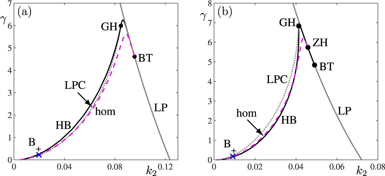
Finally, Figure 9 shows bifurcation diagrams in the $(k_2,\gamma )$ plane with values of $\mu _2=1$ (in panel (a)), and $\mu _2=1.4$ (in panel (b)). The resulting bifurcation diagrams are similar to that in Figure 7, but with higher values of $\mu _2$ . In Figure 9 the HB curve has a degenerate Hopf point GH, from which a saddle-node curve of cycles LPC emerges. All in all, upon comparing Figures 7 and 9, an increase in parameter $\mu _2$ produces extra bifurcations that favour chaotic behaviour. Indeed, the hom curve in Figure 7 is now chaotic along its entire length. Also, in Figure 9(b), an increase of $\mu _2$ favours the emergence of a ZH point. However, the bifurcation sets are “pushed” towards lower values of $k_2$ and larger values of $\gamma $ as $\mu _2$ is increased; compare the scale of the variables in Figures 7 and 9.

Figure 9

Bifurcation diagrams of (2.1) in the $(k_2,\gamma )$ plane. Parameter values are as in Figure 7, except $\mu _2=1$ in (a), and $\mu _2=1.4$ in (b).

Sample solutions for autoinducer concentration and bacterial population, along with their corresponding phase orbits, are presented in Figure 10 for representative $k_2$ and $\gamma $ parameter values from Figure 7. The stable focus shown in column (a) undergoes a bifurcation into a limit cycle in column (b) as the parameter $\gamma $ crosses the HB curve. The oscillation period further increases as $\gamma $ approaches the hom curve, as illustrated in column (c).

Figure 10

Samples of time solutions (upper panels) and corresponding phase orbits (lower panels) of system (2.1). (a) Damped oscillatory solution with a stable focus for $\gamma =2.5$ ; (b) oscillatory periodic solution with a stable limit cycle for $\gamma =2$ ; (c) spike-like periodic solution near a homoclinic orbit for $\gamma = 1.8$ . Initial conditions are chosen close to the saddle point. Parameter values: $k_2 = 0.1535$ , $\mu _1 = 0.2$ , $\mu _2 = 0.7$ , with remaining parameters as listed in Table 2.

This transition is evident in the time solutions displayed in the upper panels, where the crests and valleys of the autoinducer concentration correspond to the peaks and troughs of the bacterial population over time. In column (a), the amplitudes of both q and $m+s$ decay over time, eventually stabilizing at a steady state. In contrast, columns (b) and (c) demonstrate a progression in oscillatory behaviour, with the period lengthening and culminating in a spike-like periodic pattern right until the formation of the homoclinic orbit.

The bifurcation diagrams in Figures 8 and 9 reveal that the dynamical richness and complexity of the system are not exclusively determined by the parameters $k_2$ and $\gamma $ . Decay rate parameters also play a pivotal role in shaping the system’s behaviour. Specifically, chaotic regions and their intricate features are not restricted to the $(k_2,\gamma )$ plane but can also emerge through the gradual variation of other system parameters, highlighting the multidimensional nature of the dynamics. In particular, whenever parameters approach sufficiently close to the hom curve in its chaotic regime, one might expect the stable periodic motion to undergo multiple saddle-node and period-doubling phenomena (not shown in the bifurcation diagrams) and, ultimately, encounter regions in phase space where chaos exists. However, the chaotic solutions cannot be directly accessed through standard time integration from initial conditions due to the saddle-like nature of the hyperbolic set, which prevents it from acting as an attractor. A chaotic trajectory may be reached from the stable manifold of the saddle invariant set. A nearby orbit spends a long time “visiting” the chaotic invariant set until it manages to escape and converge to an attracting object. Furthermore, these chaotic regions in phase space are typically confined to a small neighbourhood surrounding the homoclinic curve, making the identification and characterization of transient chaos particularly challenging. The detailed exploration of these chaotic sets lies beyond the scope of the present work. For an in-depth theoretical and numerical analysis and further insights into the dynamics of these regions, the reader is referred to [Reference Aguirre, Krauskopf and Osinga1].

6 Discussion

Analysing the effect of autoinducers on bacterial populations is crucial due to their key role in the QS mechanism. We presented a model that demonstrates the interaction between autoinducers and two subtypes of bacteria. A thorough analysis of this model revealed parameter sets that lead to oscillation dynamics in both the constant autoinducer submodel and the full three-component model. The study was performed with a combination of both rigorous normal-form analysis and numerical continuation methods. Upon analysing the full system, we were able to understand how autoinducer concentrations interact with bacterial populations and influence bacterial communication triggered by these interactions.

The constant autoinducer system (3.5) shows that parameter e is inversely proportional to the autoinducer concentration $q_0$ , indicating that changes in e can impact response rates and production rates on the population. Exploring additional parameters revealed that parameter b, related to bacteria decay rates, leads to a family of limit cycles via Hopf bifurcation. By conducting two-parameter numerical continuation on parameters b and e, the $(b,e)$ plane was divided into four regions based on their dynamical events. It was observed that no synchronizing behaviour occurs for high values of e, suggesting that oscillatory behaviour may not occur below certain critical shallow threshold autoinducer concentration; this discovery agrees with QS features already recognized in some previous work [Reference Kaur, Capalash and Sharma20, Reference Li, Fu, Zhang and Wang24, Reference Taylor, Tinsley, Wang and Huang35].

Furthermore, as can be seen from Proposition 3.1, when

$$ \begin{align*} \mathcal{J}=b/(1- u_*^2/[v_*(1+Ku_*^2)]), \end{align*} $$

notice that $\text {tra}(\mathbf {J})=[(b+1)u_*^2 - v_*(1+Ku_*^2)]/[v_*(1+Ku_*^2)-u_*^2]$ and $\text {det}(\mathbf {J})=0$ , which suggest that other nonlinear events may trigger synchronizing behaviour on the bacterial population not only by means of a Hopf bifurcation. To fully understand such an implication and, in consequence, the impact of autoinducer dynamics on the population, we analysed the three-dimensional system and identified $k_2$ and $\gamma $ as key parameters for synchronizing dynamics. Through Hopf bifurcations, self-sustained oscillations were observed to emerge. A two-parameter continuation analysis revealed that these parameters play a role in the emergence of additional oscillatory behaviour and robust synchronization properties in the population. From Section 5, the identification and mapping of homoclinic bifurcations in the model are crucial for understanding the dynamic behaviour of autoinducer concentration and bacterial population interactions. The sample solutions presented in Figure 10 illustrate how the system transitions from a stable focus to oscillatory behaviour through a Hopf bifurcation as the parameter $\gamma $ crosses the HB curve. As $\gamma $ approaches the homoclinic bifurcation, the increasing oscillation period signifies a critical shift in system dynamics, leading to complex behaviours such as spike-like periodic patterns. This progression highlights the importance of recognizing homoclinic bifurcations, as they serve as pivotal points that can influence different types of oscillatory behaviour.

Moreover, it was observed that a Shilnikov homoclinic bifurcation branch originates from a Bogdanov–Takens point, leading to a Belyakov point $B_c$ that separates simple and chaotic behaviour along the homoclinic curve. Another Belyakov point $B_+$ marks the boundary between real saddle and saddle-focus steady states. By conducting a two-parameter continuation along three pivotal points on the homoclinic curve, varying parameters $\mu _1$ and $\mu _2$ (equivalent to parameter b in the constant autoinducer system), intricate dynamics were revealed resulting in resonant and additional Belyakov points. Additionally, a zero-Hopf point appears in a Hopf curve intersecting a nearby saddle-node curve. These findings support chaotic dynamics as infinitely many saddle-node, period-doubling orbits and n-homoclinic orbits—accompanied by countably many horseshoes for all $n\in \mathbb {N}$ —come to birth as well as invariant tori and invariant chaotic sets. In spite of all this rich dynamics, accessing chaotic solutions is hindered by the saddle-like nature of the hyperbolic set. Moreover, these chaotic regions are confined to a small neighbourhood around the homoclinic curve. All this prevents direct access to chaotic orbits through standard simulations.

The QS model examined in this study depicts synchronized oscillatory dynamics in bacterial populations, potentially exhibiting synchronizing characteristics. This behaviour is not only influenced by the presence of an autoinducer concentration threshold, but also underscores how elevated autoinducer levels drive pronounced peaks in bacterial population dynamics. Understanding these transitions not only enhances our comprehension of the underlying biological processes but also aids in predicting system behaviour under varying conditions, ultimately contributing to more effective modelling and control strategies in microbial systems. However, to fully understand the global picture of the QS mechanism, migration dynamics and time delays should also be considered. The inclusion of a time delay is crucial as it influences the dynamics of autoinducer reception and emission, indicating that bacteria do not react instantaneously to autoinducers (for example, see [Reference Mukherjee and Bassler29]). These aspects will be addressed in future research.