


1. Introduction
The flow past an arrangement of cylinders has been intensively studied owing to the great variety of industrial applications where this geometry appears, such as heat exchangers (Jang & Chen Reference Jang and Chen1997), electronic cooling (Alfieri et al. Reference Alfieri, Tiwari, Renfer, Brunschwiler, Michel and Poulikakos2013) and nuclear energy (Loganathan & Ganesan Reference Loganathan and Ganesan2006). The focus of these studies has been primarily on understanding the fundamental aspects of the fluid dynamics and heat transfer. The fluid's rheological characteristics and interaction with the blockage bodies have been studied less, which motivated us to perform this work.
From a geometrical point of view, the blockage ratio ( $\beta =D/H$) of the enclosure is an important parameter that modifies the flow dynamics. Indeed, three physical mechanisms must be considered to understand how the blockage ratio perturbs the flow (Rao, Sahu & Chhabra Reference Rao, Sahu and Chhabra2011). First, the walls increase the velocity gradients in the flow by increasing the blockage ratio. Second, the flow velocity increases as the blockage ratio increases owing to the decrease in the gap between the cylinder and enclosure walls. Finally, depending on the blockage ratio and interaction between the walls, vortex shedding can be promoted in the flow. Concerning these features, walls can stabilize or destabilize the flow depending on their configuration (Anagnostopoulos, Iliadis & Richardson Reference Anagnostopoulos, Iliadis and Richardson1996; Sahin & Owens Reference Sahin and Owens2004). Sahin & Owens (Reference Sahin and Owens2004) defined the stability curve of Newtonian flow past a confined cylinder for a wide range of blockage ratios,
 $0.1<\beta <0.9$. Moreover, it was demonstrated that the walls provide stability to the flow in the blockage ratio range
 $0.1<\beta <0.5$, whereas the walls tend to destabilize the flow dynamics for
 $0.5<\beta <0.9$, presenting a variety of flow behaviours depending on the blockage ratio and Reynolds number considered.
Three-dimensional flows past cylinders have also been addressed in several studies. Barkley & Henderson (Reference Barkley and Henderson1996) report a critical Reynolds number from which the flow becomes unstable to three-dimensional perturbations of  $Re=188.5$. Pralits, Giannetti & Brandt (Reference Pralits, Giannetti and Brandt2013) extend the instability analysis of non-rotating cylinders to rotating cylinders, showing that the critical Reynolds numbers decrease for this case. Recently, in Ooi et al. (Reference Ooi, Chan, Aljubaili, Mamon, Leontini, Skvortsov, Mathupriya and Hasini2020), the flow of Newtonian fluids was studied using two- and three-dimensional direct numerical simulations for
 $0.1<\beta <0.9$ and
 $120< Re<500$.
The number of cylinders, their configuration and the distance between their centres are other geometrical parameters that influence the flow dynamics (Zdravkovich Reference Zdravkovich1987; Mizushima & Suehiro Reference Mizushima and Suehiro2005; Mahír & Altaç Reference Mahír and Altaç2008; Mittal, Kottaram & Kumar Reference Mittal, Kottaram and Kumar2008; Yen, San & Chuang Reference Yen, San and Chuang2008; Carmo, Meneghini & Sherwin Reference Carmo, Meneghini and Sherwin2010; Igarashi Reference Igarashi2011; Choi, Jang & Yang Reference Choi, Jang and Yang2012). In Zdravkovich (Reference Zdravkovich1987), the flow past two circular cylinders in tandem was studied. In this work, the authors mentioned three different flow regimes related to the distance between the centres of the cylinders ( $L_{x}/D$), where
 $L_{x}$ is the distance between the centres of the cylinders, and
 $D$ is the characteristic length of the cylinders. Thus, they defined three ranges: the range
 $1< L_{x}/D<2$, where the second cylinder entirely suppresses the von Kármán street; a reattached regime for
 $2< L_{x}/D<5$, where the detached vortices from the first cylinder impact the frontal face of the second cylinder; and a co-shedding regime for
 $L_{x}/D>5$, where the vortex detachment is independent for both cylinders. Choi et al. (Reference Choi, Jang and Yang2012) found the secondary instability of the flow past two square cylinders in tandem. Here, the critical Reynolds number from the flow that moves from two-dimensional to three-dimensional was detected. In Yen et al. (Reference Yen, San and Chuang2008), the Newtonian flow of two cylinders with square shapes was studied. In that work, the authors categorized the flow as single mode, reattached mode and binary mode depending on the Reynolds number and spacing ratio between the cylinders.
The shape of the cylinders is an important parameter that modifies the flow dynamics. In this context, a square shape provides larger wake size regions and drag coefficients than circular and elliptical shapes, under a fixed Reynolds number (Sen, Mittal & Biswas Reference Sen, Mittal and Biswas2011). Thus, the blunt shape of the square cylinder favours the appearance of instabilities in the flow. Therefore, several studies of the flow past a cylinder problem have analysed the influence of a square shape on flow patterns. In Saha, Muralidhar & Biswas (Reference Saha, Muralidhar and Biswas2000), the flow transition and route to chaos for a Newtonian flow past a cylinder with a square shape was studied numerically. In that work, it can be observed that, as the Reynolds number increases, there is a flow transition from a time-dependent laminar structure to a chaotic structure through a quasi-periodic route to chaos. Patil & Tiwari (Reference Patil and Tiwari2008) determined the stability curve of the flow past a confined cylinder with a square shape, concluding that the flow past a square cylinder demonstrates a lower critical Reynolds number than flow past a circular cylinder (Choi et al. Reference Choi, Jang and Yang2012) for blockage ratios in the range  $0.1\leq \beta \leq 0.5$.
Geometric parameters are not the only ones that modify the flow dynamics. Fluid rheology also has an essential role. In this context, non-Newtonian fluids have been widely studied because they are found in numerous scientific fields, including polymers (Metzner Reference Metzner1985), the food industry (Tabilo-Munizaga & Barbosa-Cánovas Reference Tabilo-Munizaga and Barbosa-Cánovas2005) and haemodynamics (Hron, Málek & Turek Reference Hron, Málek and Turek2000). Concerning the intrinsic nonlinear behaviour of this kind of fluid, advantageous properties in heat transfer and in the development of chaotic flows for relatively low Reynolds numbers have been studied (Bharti, Chhabra & Eswaran Reference Bharti, Chhabra and Eswaran2007a,Reference Bharti, Chhabra and Eswaranb; Sahu, Chhabra & Eswaran Reference Sahu, Chhabra and Eswaran2009). In Ruz et al. (Reference Ruz, Castillo, Cruchaga and Aguirre2021), the Hopf bifurcation of non-Newtonian isothermal fluids past one and two cylinders in tandem under different blockage ratios is determined. In that work, the authors found that the critical Reynolds number decreases as the power-law index decreases. Furthermore, they determined that the critical Reynolds number could increase or decrease as the blockage ratio increases, depending on the power-law index and cylinder configuration.
In Lashgari et al. (Reference Lashgari, Pralits, Giannetti and Brandt2012), a detailed study of the flow characteristics of isothermal Carreau fluids is carried out. In that work, the authors look for the Hopf bifurcation for different power-law indices and material time constants. The authors found that the shear-thinning fluids tend to destabilize the flow in contrast to the shear-thickening flows. In Dhiman, Chhabra & Eswaran (Reference Dhiman, Chhabra and Eswaran2008), the non-Newtonian flow past a confined cylinder with a square shape was studied in detail. The authors found that the recirculation length was larger for shear-thinning fluids. In Bharti et al. (Reference Bharti, Chhabra and Eswaran2007b), the effect of the blockage ratio on the heat transfer characteristics of non-Newtonian fluids past a cylinder was studied numerically. In that work, the authors found that the average Nusselt number increases by increasing the Reynolds number, blockage ratio and Prandtl number, or by decreasing the power-law index. In Sahu, Chhabra & Eswaran (Reference Sahu, Chhabra and Eswaran2010), the forced convection of non-Newtonian flows past a confined cylinder with a square shape was studied. In that work, the influence of the Reynolds number, Prandtl number, blockage ratio and power-law index on the Nusselt number was addressed, determining that the Nusselt number increases by increasing the Reynolds number and the blockage ratio, and by decreasing the power-law index.
The non-Newtonian flows past an arrangement of cylinders have also been addressed. In Nejat, Abdollahi & Vahidkhah (Reference Nejat, Abdollahi and Vahidkhah2011), the isothermal flow of power-law fluids past two confined cylinders with a circular shape was studied for several distances between the cylinders. In that work, it was determined that the downstream cylinder does not influence the upstream cylinder for a distance between centres of  $L_{x}/D\geq 3D$. Conversely, the downstream cylinder is entirely influenced by the upstream cylinder as the Reynolds number increases for a fixed distance between the centres and power-law index. Bouaziz, Kessentini & Turki (Reference Bouaziz, Kessentini and Turki2010) studied the mixed convection of non-Newtonian flows past a cylinder with a square shape for
 $\beta =1/8$. In that work, it was determined that the critical Reynolds number from the flow moves from stationary to time-dependent depending on the Reynolds number, Richardson number and power-law index. In Nikfarjam & Sohankar (Reference Nikfarjam and Sohankar2013), the non-Newtonian flow past an arrangement of two cylinders with a square shape in tandem was performed for a fixed distance between centres of
 $L_{x}/D=4D$ and Prandtl number of
 $Pr=0.7$. In that work, the authors observed that the Nusselt number increases by decreasing the power-law index and decreases by increasing the power-law index.
A literature review indicates that non-isothermal flows over tandem arrangements of cylinders, circular or square, have not been addressed deeply for shear-thinning fluids, and, in the same way, the effect of the blockage ratio for this type of fluid has not been developed in detail for moderate and high values either. Hence, the novelty of this work is to perform an exhaustive numerical analysis that considers the shear-thinning characteristics of different power-law fluids and the effect of the blockage ratio on the heat transfer and fluid dynamics. Numerical simulations are performed using an in-house code based on the finite element method, which has proven to be robust and accurate in Newtonian and non-Newtonian problems (Castillo & Codina Reference Castillo and Codina2019; Abugattas et al. Reference Abugattas, Aguirre, Castillo and Cruchaga2020; González, Castillo & Cruchaga Reference González, Castillo and Cruchaga2020; Ruz et al. Reference Ruz, Castillo, Cruchaga and Aguirre2021).
This work is organized as follows. In § 2, the governing equations and power-law model are presented. In § 3, the set-up of the analysed problem is defined; a brief description of the numerical method used to solve the problem is presented in § 4.1. In §§ 4.3 and 5, the principal results of this work are presented, including a numerical validation of the code and method used. The results include a wide range of power-law indices and blockage ratios. Finally, the main conclusions are summarized in § 7.
2. Governing equations
In this work, the forced convection flow of shear-thinning fluids is studied. The problem is governed by the momentum, continuity and energy equations, which are stated as follows:
 $$\begin{gather} \rho\frac{\partial\boldsymbol{u}}{\partial t} +\rho\boldsymbol{u} \boldsymbol{\cdot} \boldsymbol{\nabla}\boldsymbol{u} -\boldsymbol{\nabla}\boldsymbol{\cdot} (2\eta\boldsymbol{\nabla}^{s}\boldsymbol{u} )+\boldsymbol{\nabla} p=\boldsymbol{f}, \end{gather}$$
 $$\begin{gather}\boldsymbol{\nabla}\boldsymbol{\cdot}\boldsymbol{u}=0, \end{gather}$$
 $$\begin{gather}\rho c_{p}\frac{\partial T}{\partial t}+\rho c_{p}\boldsymbol{u} \boldsymbol{\cdot}\boldsymbol{\nabla} T-k\Delta T=Q, \end{gather}$$
where  $\boldsymbol {u}$ is the velocity,
 $p$ is the pressure and
 $T$ is the temperature field. The fluid properties
 $\eta$,
 $\rho$,
 $k$ and
 $c_{p}$ represent the apparent viscosity, density, thermal conductivity and heat capacity of the fluid, respectively. The terms
 $\boldsymbol {f}$ and
 $Q$ on the right-hand side represent the external body force and a heat source, respectively, which are equal to zero for this work. The above equations are solved sequentially with appropriate initial and boundary conditions, that is, (2.1) and (2.2) are solved in the first step using a monolithic approach to obtaining
 $\boldsymbol {u}$ and
 $p$, and then, in a second step, (2.3) is calculated to define the temperature field.
With respect to the rheological behaviour of the fluid, the power-law constitutive model is used, which is defined as follows:
 \begin{equation} \eta=m\dot{\boldsymbol{\gamma}}^{n-1}, \end{equation}
where  $\dot {\gamma }=\sqrt {(\boldsymbol {\dot {\gamma }:\dot {\gamma }})/2}$ represents the magnitude of the rate-of-deformation tensor
 $\boldsymbol {\dot {\gamma }} = \boldsymbol {\nabla }\boldsymbol {u} +(\boldsymbol {\nabla }\boldsymbol {u})^{\textrm {T}}$,
 $m$ represents the consistency index and
 $n$ is the power-law index of the fluid. The reason to use this model is to get trends that can be useful to understand more complex models, like Carreau or Herschel–Buckley, which is a combination of the Bingham model and the power-law one. The inherent problem of the power-law model is the prediction of zero viscosity values as
 $\dot {\gamma }\rightarrow 0$, when
 $n<1$. In this work, a cutoff parameter is used to prevent the apparent viscosity from being less than
 ${m}/{10\,000}$.
The Poiseuille profile of power-law fluids, which reads as
 \begin{equation} U(y,n)=\left(\frac{2n+1}{n+1}\right)U_{avg}\left\{ 1-\left|\frac{2y}{H}\right|^{({n+1})/{n}}\right\}, \end{equation}
is used as boundary velocity condition, where  $y$ represents the vertical axis (see figure 1),
 $H$ is the height of the enclosure and
 $U_{avg}$ represents the average velocity. Note that this profile allows us to compare the different fluids in a developed flow condition for a fixed Reynolds-number value, ensuring that the results are not perturbed by numerical effects.
Schematic representation of the flow phenomenon under study.

The dimensionless numbers for power-law fluids must be redefined in terms of the constitutive model parameters. The Reynolds number ( $Re$) and Prandtl number (
 $Pr$) for power-law fluids are defined as follows:
 \begin{equation} Re=\frac{\rho U_{avg}^{2-n}D^{n}}{m} , \quad Pr=\frac{mC_{p}}{k}\left(\frac{U_{avg}}{D}\right)^{n-1}. \end{equation}
To determine the rate of heat transfer of the square cylinders, the Nusselt number is computed. The local and average Nusselt numbers are calculated as follows:
 \begin{equation} Nu(s)={-}\frac{\partial T}{\partial n_{s}} , \quad \overline{Nu}=\frac{1}{L}\int_{L}Nu(s)\,\textrm{d}s, \end{equation}
where  $n_{s}$ is the unit vector normal to the surface of the cylinder.
3. Problem statement
In this work, the forced convection of power-law flows past two confined square cylinders in tandem is performed numerically. The problem is solved for the two- and three-dimensional cases. In figure 1, a problem sketch along with its boundary conditions is presented for the two-dimensional case. The three-dimensional problem is a direct extension of the plane problem with a width equal to the height (square section). It is necessary to define the blockage ratio  $\beta =D/H$, where
 $D$ is the length of the cylinder, taken as unitary (
 $D=1$), and
 $H$ is the height of the enclosure. To define the total length of the pipe, we require the upstream distance (
 $L_{u}=12D$) and downstream distance (
 $L_{d}=15D$). The values used in this work ensure that the boundary conditions do not perturb the fluid dynamics (Dhiman et al. Reference Dhiman, Chhabra and Eswaran2008; Ruz et al. Reference Ruz, Castillo, Cruchaga and Aguirre2021). Because different blockage ratios are used, the height of the pipe (and width in the three-dimensional case) are defined as
 $H=D/\beta$. Concerning the gap between the cylinders, a value of
 $S=3D$ is used. The chosen gap is not arbitrary; it has been derived from several articles that have postulated a strong fluid dynamics interaction for cylinder arrangements with distances between centres of
 $2\leq S \leq 4$ (Zdravkovich Reference Zdravkovich1987; Carmo et al. Reference Carmo, Meneghini and Sherwin2010; Nejat et al. Reference Nejat, Abdollahi and Vahidkhah2011). From the physical point of view, there is a vortex detachment of the fluid in the first cylinder that impacts the front surface of the second cylinder, generating complex fluid dynamics in the gap between the cylinders. In the present work, this geometrical configuration is studied for power-law fluids, including forced convection.
For the velocity boundary conditions, the power-law Poiseuille profile is defined at the inlet ( $x=0$), no-slip conditions are defined at the enclosure walls or cylinder surfaces, and an open flow condition is set at the outlet (
 $x=32D$). For temperature conditions, a constant temperature of
 $T_{\infty }=0$ is set at the inlet, an adiabatic condition is imposed at the enclosure walls, and a constant temperature of
 $T_{W}=1$ is applied at the cylinder surfaces.
4. Numerical parameters and validation
4.1. Numerical method
The governing equations were solved using a recently proposed stabilized variational multiscale (VMS) finite element formulation (Castillo & Codina Reference Castillo and Codina2019), which allows the approximation of convective dominant cases and even turbulent flows without the inclusion of an additional turbulent model González et al. (Reference González, Castillo and Cruchaga2020). This formulation modifies the standard discrete Galerkin formulation by adding terms designed to enhance the stability without upsetting the accuracy and ensuring that the convergence rates of the method are optimal for velocity and pressure. The method can be understood as an implicit large-eddy simulation that is derived from the VMS framework and has an optimal dissipative structure (Castillo & Codina Reference Castillo and Codina2019). For P1 elements, the rates of convergence of velocity and pressure are two and one, respectively (González et al. Reference González, Castillo and Cruchaga2020). The method used consists of splitting the velocity subscale into two terms, unlike traditional VMS methods, having a non-residual term-by-term structure that is obtained by neglecting all cross local inner product terms that do not provide stability. The details of the dissipative structure of this method, including its mathematical structure, numerical verifications and the numerical treatment of the nonlinearities, are provided in Castillo & Codina (Reference Castillo and Codina2019) and González et al. (Reference González, Castillo and Cruchaga2020).
The time derivative is discretized using the second-order backward scheme, for both the momentum and the energy equations, as follows:
 \begin{equation} \frac{\partial
\varphi_h^{\,j+1}}{\partial t}
=\frac{3\varphi_h^{\,j+1}-4\varphi_h^{j}+\varphi_h^{\,j-1}}{2
\delta t} +{O}(\delta t^2),
\end{equation}
where  $\delta t$ corresponds to the size of a uniform partition of the time interval where the problem is solved, while
 ${O}(\cdot )$ represents the order of integration of the scheme. The index
 $j$ indicates the time step where the function
 $\varphi$ is being approximated.
4.2. Numerical parameters
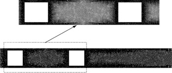
An adequate mesh choice is essential for reproducing any problem. The grid should be capable of capturing velocity gradients to ensure a correct approximation of the viscosity, as well as to accurately define the complex unsteady behaviour developed by the flow. In this work, a non-structured mesh composed of linear triangular (P1) elements was used. The mesh was refined near the walls and over the square cylinders, as can be seen in figure 2. To ensure that numerical results are independent of the used mesh, a convergence study based on the calculation of the drag coefficient and Nusselt numbers of both cylinders was performed for  $Pr=10$, considering the most blocked case (
 $\beta =0.8$) and the lowest power-law index,
 $n=0.25$, which represents the most demanding case of our study from the physical and computational points of view.
Mesh representation at  $\beta =0.8$.

Three meshes, referred to as  $G_{i}$,
 $i=1,\ldots,3$, with the details reported in table 1, were tested for this case. In table 1,
 $G_{1}$ represents the most refined mesh and
 $G_{3}$ represents the coarser mesh. From the results, it can be observed that the difference in the results between grids
 $G_{1}$ and
 $G_{2}$ is small. For this reason, subsequent simulations were performed using grid
 $G_{2}$, which provides accuracy and moderate computational requirements. As the domain depends on the blockage ratio, grid
 $G_{2}$ is only used as a base to define the other blockage cases (
 $\beta =0.5$ and 0.66). The number of elements used for each case is reported in table 2, where details of the elements used in the regions far from and close to the cylinders are included.
Mesh convergence test evaluating the drag and Nusselt number.

Mesh details based on blockage ratios.

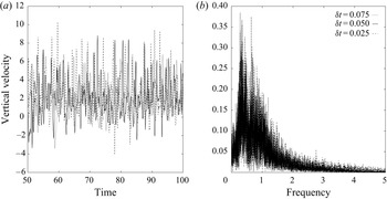
Because dynamic solutions are analysed, the effect of the time-step value ( $\delta t$) is also evaluated. For this reason, the influence of three different time-step sizes
 $\delta t_{1}=0.025$,
 $\delta t_{2}=0.05$ and
 $\delta t_{3}=0.075$ on the velocity evolution and its corresponding fast Fourier transform (FFT) were tested for the most critical case of
 $\beta = 0.8$ and
 $n=0.25$, which are reported in figure 3. In addition, table 3 shows the values of the first three dominant frequencies obtained using the three time-step values. From these values, we can see that the differences of using
 $\delta t_{1}$ instead of
 $\delta t_{2}$ is less than
 $5\,\%$. From the quality of the results and the computational resources,
 $\delta t_{2}$ was selected.
(a) Vertical velocity and (b) FFT convergence at  $\beta = 0.8$ and
 $n=0.25$ evaluated in
 $Z_{2}$.

First three dominant frequencies for each time step

4.3. Numerical validation
The VMS method used in this work has demonstrated robustness and accuracy in different numerical scenarios (Castillo & Codina Reference Castillo and Codina2019; González et al. Reference González, Castillo and Cruchaga2020; Ruz et al. Reference Ruz, Castillo, Cruchaga and Aguirre2021). In our case, it is used to solve a new problem that involves the forced convection of power-law fluids.
Through numerical validation, the flow over a square cylinder with aiding buoyancy is solved in this subsection by comparing the results obtained in the work with those reported in Sharma, Dhiman & Kumar (Reference Sharma, Dhiman and Kumar2013). The results of the average drag coefficients and average Nusselt numbers are presented in table 4 for a wide range of power-law indices at  $Re=30$,
 $Pr=50$,
 $Ri=1.0$ and
 $\beta =0.25$. From the results, it can be observed that the errors were less than
 $3.1\,\%$ in the drag coefficient value and less than
 $2\,\%$ in the Nusselt-number value. These results confirm the correct implementation of the power-law model and the accuracy of the VMS method.
Validation of drag and Nusselt numbers for different power-law indices at  $\beta =0.25$,
 $Re=30$,
 $Ri=1.0$ and
 $Pr=50$.

The relative errors reported in the above tables were calculated based on  $| ({\text {value} _{{article}}-\text {value} _{reference}})/{\text {value}_{article}} |\,\%$.
5. Numerical results
In this section, the confined flow over two square cylinders in tandem is studied for power-law fluids. Three blockage ratios of  $\beta =0.50$,
 $0.66$ and
 $0.80$ are used to solve shear-thinning fluids characterized by a power-law index in the range
 $0.25\leq n \leq 1.0$. The non-dimensional numbers for all cases are
 $Re=100$ and
 $Pr=10$. The chosen Prandtl number can describe water-based solutions of non-Newtonian fluids, which are widely used in the context of electronic refrigeration and microchannel devices (Parvin, Alim & Hossain Reference Parvin, Alim and Hossain2012; Akbari et al. Reference Akbari, Toghraie, Karimipour, Marzban and Ahmadi2017; Sajadifar, Karimipour & Toghraie Reference Sajadifar, Karimipour and Toghraie2017).
Since all cases in the study are nonlinear, each problem is solved interactively for each time step to achieve a convergence error smaller than  $10^{-6}$ in the discrete
 $L^{2}$ norm of the unknowns. In general, no more than 10 iterations are needed to ensure this convergence.
5.1. Fluid dynamics
Based on several studies (Bharti et al. Reference Bharti, Chhabra and Eswaran2007a,Reference Bharti, Chhabra and Eswaranb; Ruz et al. Reference Ruz, Castillo, Cruchaga and Aguirre2021), the flow patterns in confined flow over bodies depend on the blockage ratio and power-law index, and there is a strong relationship between these parameters. To further illustrate this fact, the streamlines and viscosity fields for representative cases are presented in this section.
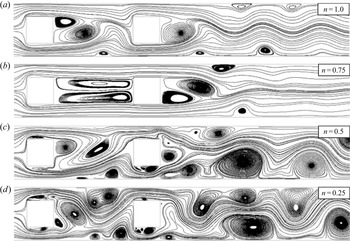
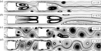
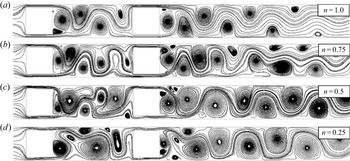
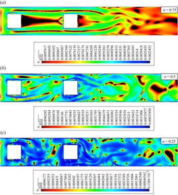
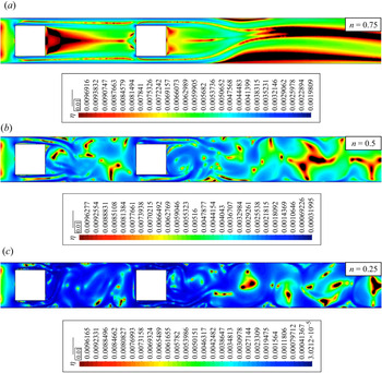
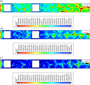
The effects of the blockage ratios and power-law indices on the fluid dynamics of the problem are illustrated in figures 4, 5 and 6, for  $\beta =0.5$,
 $0.66$ and
 $0.80$, respectively. Figure 4 indicates that, for a fixed blockage ratio, the shear-thinning behaviour drastically changes the fluid dynamics. For all the cases presented in the figure, a clear time dependence of the flow can be observed, with a more complex behaviour as the power-law index decreases. The same tendency is maintained for the other two blockage ratios. Comparing
 $\beta =0.5$ and
 $\beta =0.80$, it can be observed that the recirculation zone behind the cylinder is shorter in the most blocked case, with a von Kármán street much more defined in the case of
 $\beta =0.8$. This is due to the proximity of the walls, which prevents the flow from moving in the cross direction. In addition, an increase in the horizontal velocity occurs because of the decrease in the section through which the fluid flows.
Instantaneous streamlines at arbitrary instants  $t$ after the transient initial flow at
 $\beta =0.5$.

Instantaneous streamlines at arbitrary instants  $t$ after the transient initial flow at
 $\beta =0.66$.

Instantaneous streamlines at arbitrary instants  $t$ after the transient initial flow at
 $\beta =0.8$.

The fluid behaviour, given principally by the power-law index value, also changes the flow patterns. From figures 4, 5 and 6, it can be observed that the flow dynamics is increased by decreasing the power-law index, even for a fixed  $\beta$ value. However, for
 $\beta =0.5$ and
 $0.66$, and for
 $n=0.75$, the opposite tendency was found. In the case of
 $\beta = 0.66$ with
 $n = 0.75$, the appearance of an asymmetric stationary solution is evident, which is framed in the context of the pitchfork bifurcation. Although this phenomenon is interesting, its analysis is beyond the scope of the present work. Despite these particular cases, an increase in the fluid dynamics as the power-law index decreases is clear. This is because the walls increase the shear stresses, with the corresponding increase in the shear-thinning behaviour of the fluids, which is greater as the power-law index decreases.
The streamlines displayed in figures 4–6 help to visualize how dynamic the flow is for the different cases studied. Conversely, the mean velocity profiles displayed in figure 7 are useful for understanding the effect of the power-law index on the mean flow dynamics. The mean velocity profiles are computed at the two control sections ( $Z_{1}$ and
 $Z_{2}$) indicated in figure 1, considering all power-law indices and
 $\beta =0.5$ and
 $0.8$. The time-averaged velocity profiles indicate that the maximum velocities increase by decreasing the power-law index, regardless of the location and blockage ratio considered. Moreover, the velocity profiles indicate negative values near the enclosure walls for
 $n=0.5$ and
 $0.25$, which is related to the existence of recirculation regions and vortex shedding zones. Finally, both figures 1 and 7 indicate greater velocity gradients near the enclosure walls, and become more pronounced as the power-law index decreases.
Averaged velocity profile at control sections: (a) in the middle of the gap between the cylinders,  $Z_{1}$, and (b) at
 $1.5D$ from the centre of the downstream cylinder,
 $Z_{2}$.

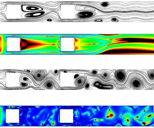
Figures 8, 9 and 10 display the viscosity fields for representative instants of the non-Newtonian flows evaluated in this subsection. The coloured regions indicate the fluid regions that have suffered a decrease in the value of apparent viscosity with respect to the viscosity at  $\dot {\gamma }=1$; the black zones represent the regions that have suffered an increase in
 $\eta$ with respect to the viscosity at
 $\dot {\gamma }=1$. From these results, it can be observed that the fluid thinning is greater near the enclosure and cylinder walls. Moreover, in the majority of cases, the fluid thinning covers the entire domain in the region between the cylinders. However, the coverage percentage in the downstream cylinder's wake depends on the blockage ratio and power-law index. In particular, it can be observed that, with a decrease in the power-law index or increase in the blockage ratio, the coverage percentage increases. In the first part, the fluid thinning is greater as the power-law index decreases because of its nonlinear nature. Conversely, fluid thinning is greater as the blockage ratio increases because it causes higher velocities and greater fluid shear rates.
Instantaneous viscosity fields at arbitrary instants  $t$ after the transient initial flow at
 $\beta =0.5$ (coloured regions, thinning regions; black regions, thickening regions).

Instantaneous viscosity fields at arbitrary instants  $t$ after the transient initial flow at
 $\beta =0.66$ (coloured regions, thinning regions; black regions, thickening regions).

Instantaneous viscosity fields at arbitrary instants  $t$ after the transient initial flow at
 $\beta =0.8$ (coloured regions, thinning regions; black regions, thickening regions).

The viscosity profiles are directly related to the velocity profiles. In figure 11, the mean viscosity profiles at the wake control zone of each cylinder are presented ( $Z_{1}$ and
 $Z_{2}$). From figure 11, it can be noted that the apparent viscosity decreases as the power-law index decreases, and it is similar at both locations. For example, if we use the average of the mean apparent viscosity profiles at
 $Z_{1}$, we obtain a value of
 $0.005164$ and
 $0.001403$ for
 $n=0.75$ and
 $n=0.25$, respectively. The same tendency is maintained at
 $Z_{2}$, with values of
 $0.005081$ and
 $0.001282$ for the same power-law indices.
Averaged viscosity profile at control sections: (a) in the middle of the gap between the cylinders,  $Z_{1}$, and (b) at
 $1.5D$ from the centre of the downstream cylinder,
 $Z_{2}$.

5.2. Route to chaos
In the above section, the effects of the blockage ratio and shear-thinning behaviour of the fluids were discussed using streamlines and apparent viscosity fields. The aim of this section is to analyse in more detail the change from laminar to chaotic solutions using dynamic systems analysis tools.
The route to chaos of the cases discussed herein is studied qualitatively by their frequency spectrum, phase diagrams and Poincaré sections. In addition, the largest Lyapunov exponent is calculated to evaluate the chaos quantitatively. The described tools are evaluated at a control point situated in the midplane at a distance of  $3D$ from the centre of the last cylinder. For specific tools (Poincaré section and Lyapunov exponent), it is necessary to reconstruct the system attractor. For this purpose, the attractor reconstruction is performed by the Takens embedding theorem (Takens Reference Takens1981; Noakes Reference Noakes1991). All the analyses are performed using the vertical velocity evolution of the corresponding graphs (cross-flow component). The optimal delay and dimension are calculated according to the methods of mutual information (Fraser & Swinney Reference Fraser and Swinney1986) and false neighbours (Kennel, Brown & Abarbanel Reference Kennel, Brown and Abarbanel1992), respectively.
To avoid overloading this section with the results, the extreme cases of blocking ( $\beta =0.5$ and
 $\beta =0.8$) are analysed.
5.2.1. Velocity evolution and frequency spectrum
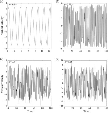
The vertical velocity evolution graphs for  $\beta =0.5$ and
 $\beta =0.8$ are displayed in figures 12 and 13, respectively. From the results, it can be observed that the flow is time-dependent in all cases. However, there is a transition from a periodic evolution to an aperiodic evolution by decreasing the power-law index, regardless of the blockage ratio considered. In addition, it can be observed that the blockage ratio promotes the appearance of more frequencies (qualitatively), which suggests that the large blockage ratios favour the appearance of flow instabilities.
Evolution of vertical velocity at  $\beta =0.5$ for (a)
 $n=1.0$, (b)
 $n=0.75$, (c)
 $n=0.5$ and (d)
 $n=0.25$.

Evolution of vertical velocity at  $\beta =0.8$ for (a)
 $n=1.0$, (b)
 $n=0.75$, (c)
 $n=0.5$ and (d)
 $n=0.25$.

One of the most commonly used tools for analysing dynamic signals is the FFT. In figures 14 and 15, the frequency spectra of the velocity graphs (figures 12 and 13) are presented. In general, it can be observed that the number of active frequencies increases as the power-law index decreases or the blockage ratio increases. The Newtonian cases have a single dominant frequency for all blockage ratios. Conversely, the flows with shear-thinning behaviour are more chaotic, demonstrating dense spectra for  $n=0.5$ and
 $n=0.25$. In the middle, the flow with a power-law index of
 $n=0.75$ and
 $\beta =0.5$ has two dominant frequencies along with other frequencies, which are a linear combination of them (
 $a_{1}\,f_{1}+a_{2}\,f_{2}$) and a dense spectrum for
 $\beta =0.8$. The increase in the number of active frequencies from a single frequency (
 $n=1.0$) to two dominant frequencies (
 $n=0.75$) for
 $\beta =0.5$ suggests a quasi-periodicity route to chaos, which is consistent with the results reported in the literature for the flow past a single square cylinder (Saha et al. Reference Saha, Muralidhar and Biswas2000). Moreover, the jump between a single frequency (
 $n=1.0$) to a broadened spectrum of frequencies (
 $n=0.75$) for
 $\beta =0.8$ indicates that there is a greater power-law index
 $n>0.75$ for which the flow has two dominant frequencies. In the case of
 $n=0.5$, it can be appreciated that the flow has a broadened spectrum of frequencies regardless of the blockage ratio. Finally, the results for
 $n=0.25$ have a broadened spectrum of frequencies for all blockage ratios, greater than those reported for the other power-law indices.
Fourier transform at  $\beta =0.5$ for (a)
 $n=1.0$, (b)
 $n=0.75$, (c)
 $n=0.5$ and (d)
 $n=0.25$.

Fourier transform at  $\beta =0.8$ for (a)
 $n=1.0$, (b)
 $n=0.75$, (c)
 $n=0.5$ and (d)
 $n=0.25$.

5.2.2. Phase diagram
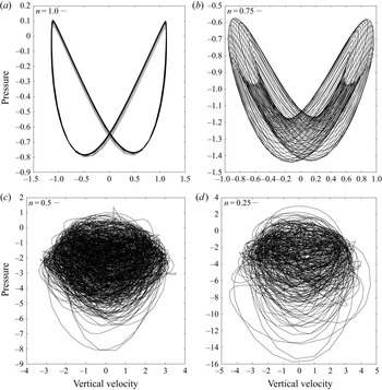
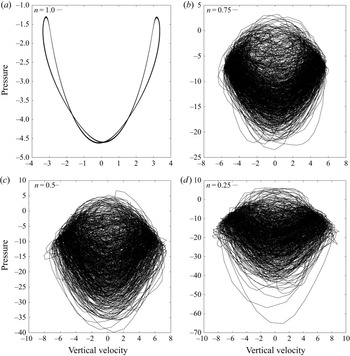
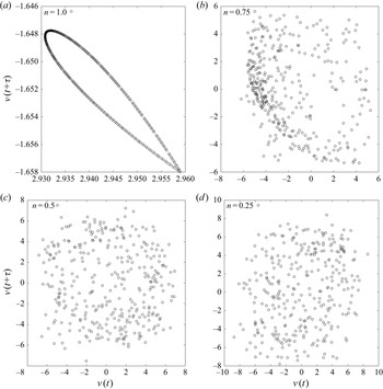
According to the shape of the phase diagram, the nature of the system attractor can be evaluated, which can be periodic with single or multiple frequencies or chaotic. Figures 16 and 17 display the phase diagrams for the different power-law indices under study and for  $\beta =0.5$ and
 $\beta =0.8$, respectively. The Newtonian cases demonstrate an organized closed trajectory, which means a periodic nature. However, it must be noted that the trajectory is deformed by increasing the blockage ratio. The case for
 $n=0.75$ indicates marked differences based on the blockage ratio under study. The phase diagram for
 $\beta =0.5$ indicates the flow's quasi-periodic nature at this power-law index and blockage ratio. For
 $\beta =0.8$, chaotic flows are obtained for all shear-thinning fluids. This indicates that it is possible to obtain chaotic states at low Reynolds numbers using high blockage ratios and low power-law indices.
Phase diagram of vertical velocity versus pressure at  $\beta =0.5$ for (a)
 $n=1.0$, (b)
 $n=0.75$, (c)
 $n=0.5$ and (d)
 $n=0.25$.

Phase diagram of vertical velocity versus pressure at  $\beta =0.5$ for (a)
 $n=1.0$, (b)
 $n=0.75$, (c)
 $n=0.5$ and (d)
 $n=0.25$.

5.2.3. Poincaré section
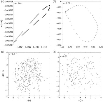
The Poincaré section represents a mapping of a reconstructed attractor with the same topological properties as the original system attractor (Berge, Pomeau & Vidal Reference Berge, Pomeau and Vidal1984; Manneville Reference Manneville2010). This dynamic system tool allows us to understand the behaviour of systems with more than three degrees of freedom. The Poincaré section based on the power-law indices and for blockage ratios of  $\beta =0.5$ and
 $0.8$ are presented in figures 18 and 19, respectively. In particular, the results displayed correspond to a time delay of
 $\tau =0.4$. For all Newtonian cases, where the flow is periodic, the Poincaré section is orderly and has a closed trajectory, which represents the laminar nature of the flow. The case of
 $n=0.75$ indicates a deformed organized Poincaré section at
 $\beta =0.5$ corresponding to the quasi-periodic regime; for
 $\beta =0.8$, the Poincaré section indicates a disorganized behaviour, suggesting that the flow is in a chaotic regime. Finally, the Poincaré sections for power-law indices
 $n\leq 0.5$ have disorganized patterns, regardless of the blockage ratio considered.
Poincaré section at  $\beta =0.5$ for (a)
 $n=1.0$, (b)
 $n=0.75$, (c)
 $n=0.5$ and (d)
 $n=0.25$.

Poincaré section at  $\beta =0.8$ for (a)
 $n=1.0$, (b)
 $n=0.75$, (c)
 $n=0.5$ and (d)
 $n=0.25$.

5.2.4. Lyapunov exponents
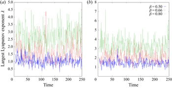
In this section, a quantitative analysis of the chaos is performed by computing the largest Lyapunov exponents of the specific cases under study. The Lyapunov exponent is the time average of the local divergence rate of the close trajectories. Indeed, the flow is chaotic if the largest Lyapunov exponent is positive, which means that the trajectories diverge from each other (Manneville Reference Manneville2010; Strogatz Reference Strogatz2018). The largest Lyapunov exponents are calculated using the algorithm proposed in Wolf et al. (Reference Wolf, Swift, Swinney and Vastano1985). Figure 20 displays the largest Lyapunov exponent in the critical cases of  $n=0.25$ and
 $n=0.5$ for all blockage ratios. The results demonstrate positive values for all cases, and that the increase in the largest Lyapunov exponent increases by increasing the blockage ratio.
Largest Lyapunov exponent based on blockage ratio and power-law index: (a)  $n=0.5$ and (b)
 $n=0.25$.

An analysis based on Lyapunov exponents allows the characterization of the flow regimes concerning the power-law indices and blockage ratios, as presented in table 5. In this table, letter L indicates a laminar time-dependent regime with a single frequency, Q is a laminar time-dependent regime with two dominant frequencies, SA is an asymmetric stationary regime and C is a chaotic regime. The results indicate that the flow goes from laminar to chaotic by decreasing the power-law index, regardless of the blockage ratio considered. Furthermore, the power-law index for those where the flow begins to be chaotic increases as the blockage ratio increases. Notwithstanding the above, the differences in the Lyapunov exponents were small between the critical blockage ratios and power-law indices. This result suggests that the flow dynamics is similar at low power-law indices and high blockage ratios.
Classification of flow regimes: unsteady state with a single frequency (L), steady asymmetric state (SA), unsteady state with two dominant frequencies (Q) and chaotic flow (C).

5.3. Heat transfer
In this section, the dependence of the average Nusselt numbers and mean temperature profiles concerning  $n$ and
 $\beta$ are discussed.
Temperature profiles allow quantification of the influence of the flow dynamics on the heat transfer enhancement. In addition, they are related to the average Nusselt number. To illustrate these characteristics, figure 21 displays the mean temperature profiles at  $Z_{1}$ and
 $Z_{2}$, considering all power-law indices and
 $\beta =0.8$. From the results, one can observe that the temperature profile increases as the power-law index decreases because of the increase in the heat convection by decreasing the power-law index. Furthermore, the temperature profile is higher in the wake of the second cylinder, which is logical because of the additional heat contribution of the second square cylinder. Moreover, as can be observed below, these increases are consistent with the increase in the average Nusselt number as the power-law index decreases. Thus, if we consider the average of the mean temperature profiles at
 $Z_{1}$, we obtain a value of
 $0.106$ and
 $0.148$ for
 $n=1.0$ and
 $n=0.25$, respectively, which means an increase of
 $39.62\,\%$. The same tendency is maintained at
 $Z_{2}$, with values of
 $0.241$ and
 $0.292$, for the same power-law indices, which means an increase of
 $21.16\,\%$.
Averaged temperature profile at control sections: (a) in the middle of the gap between the cylinders,  $Z_{1}$, and (b) at
 $1.5D$ from the centre of the downstream cylinder,
 $Z_{2}$.

The variation of the average Nusselt number with respect to  $n$ and
 $\beta$ is displayed in figure 22 for the first (upstream) and second (downstream) square cylinders at
 $Pr=10$. The illustration of the Prandtl-number influence in figure 23 displays an additional study case for
 $Pr=100$. The average Nusselt-number dependences based on the flow parameters are described below.
Variation of averaged Nusselt number at  $Pr=10$ for (a) upstream square cylinder and (b) downstream square cylinder.

Variation of averaged Nusselt number at  $Pr=100$ for (a) upstream square cylinder and (b) downstream square cylinder.

From §§ 5.2 and 5.3, the strong influences of the blockage ratio ( $\beta$) and power-law index (
 $n$) on the fluid dynamics were demonstrated. Here, the influence of these parameters on the average Nusselt numbers is discussed. From figures 22 and 23, it can be noted that Nusselt number increases as blockage ratio increases or power-law index decreases. Furthermore, from figures 22 and 23, it can be observed that all Nusselt-number curves exhibit nonlinear behaviour. The slope changes in the curves are directly related to the flow regime, which changes from laminar to chaotic, decreasing the power-law index. Finally, it can be observed that the differences in the Nusselt numbers for the different blockage ratios are decreased as the power-law index decreases for both cylinders. This is because the flow dynamics is similar at low power-law indices for the different blockage ratios under study.
Regarding the values of the Nusselt number obtained for the first and second cylinder, it can be noted that the upstream cylinder influences the average Nusselt number of the downstream cylinder. On the one hand, the first cylinder perturbs the fluid dynamics of the flow, generating a vortex detachment that favours fluid mixing. On the other hand, the preheating produced by the first cylinder on the flow reduces the temperature gradient between the hot cylinder and the flow. The overlay effect of the increase of mixing capacity and the decrease in the temperature gradient determines the heat transfer coefficient. The increase of mixing capacity is dominant for high blockage ratios regarding the decrease in the temperature gradient. The same occurs for the lowest values of  $n$. This behaviour could be helpful in the frame of microchannel devices where the blockage ratio is important, and the use of shear-thinning nanofluids could be recommendable.
Finally, the influence of the Prandtl number on the average Nusselt number is displayed in figures 22 and 23. From these results, it can be observed that, for a fixed blockage ratio, Reynolds number and power-law index, the Nusselt number increases when the Prandtl number increases. This is because there is a decrease in the thermal boundary layer with an increase in the Prandtl number. In addition, from a non-Newtonian point of view, shear-thinning fluids are characterized by a decrease in the boundary layers as the power-law index decreases, producing narrower boundary layer profiles (similar to turbulent profiles), which also influences the heat transfer process and increases the Nusselt numbers.
6. Three-dimensional flow
In this section, we extend the study to three dimensions. Because the three-dimensional cases require large computational times, we only solve the case of  $\beta =0.8$ for all power-law indices.
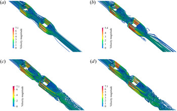
Figure 24 displays the streamlines for the three-dimensional cases. From these results, it can be observed that the flow goes from a steady ( $n=1.0$ and
 $n=0.75$) to a time-dependent (
 $n=0.5$ and
 $n=0.25$) behaviour when the power-law index is decreased. Although these results are consistent with the results reported for the two-dimensional cases, the presence of the new walls suppresses vortex shedding. Despite the above, it can be observed that the flow has a highly dynamic structure for
 $n=0.25$, which verifies the strong influence of the power-law index on the flow dynamics and the capability of shear-thinning fluids to promote chaotic flows.
Instantaneous streamlines for  $\beta =0.8$ – isometric view for (a)
 $n=1.0$, (b)
 $n=0.75$, (c)
 $n=0.5$ and (d)
 $n=0.25$.

The tracking of the velocity components for the time-dependent cases ( $n=0.5$ and
 $n=0.25$) evaluated at the wake of the second cylinder (in the centre of plane
 $Z_{2}$) is presented in figure 25. From this figure, it is clear how the flow becomes more dynamic for the lower power-law index, considering that the cases
 $n = 0.75$ and
 $n = 1.0$ were stationary.
Evolution of velocity components over time at  $\beta =0.8$ for (a)
 $n=0.5$ and (b)
 $n=0.25$.

Finally, a comparison is performed between the average Nusselt numbers. Thus, the average Nusselt number for the first cylinder is equal to  $86.57$ and
 $92.67$ for
 $n=1.0$ and
 $n=0.25$, respectively, which indicates a Nusselt-number increase of
 $7.04\,\%$. In the same manner, this trend is maintained in the second cylinder, having Nusselt-number values of
 $63.51$ for
 $n=1.0$ and
 $74.90$ for
 $n=0.25$, which means an increase of
 $17.91\,\%$. This last result confirms the capability of shear-thinning fluids to enhance heat transfer.
7. Conclusions
In this study, the forced convection of shear-thinning power-law fluids in tandem with two square confined cylinders was studied numerically. The effects of the blockage ratio of the enclosure and the power-law index of the fluid on the dynamics of the flow and on the heat transfer were investigated in detail for a fluid characterized by a Prandtl number equal to 10. The following points can be highlighted:
(i) Shear-thinning behaviour of the fluid promotes chaotic flows at low Reynolds numbers, increasing the heat transfer coefficients with respect to Newtonian fluids.
(ii) Higher blockage ratios promote the generation of chaotic flows in shear-thinning power-law fluids, increasing the heat transfer coefficients with respect to Newtonian fluids.
(iii) The effects of the blockage ratio and the shear-thinning behaviour of the fluid are complementary, and enhance flow mixing and heat transfer.
(iv) The studied cases have a quasi-periodic route to chaos as the power-law index decreases for the blockage ratios, Reynolds numbers and Prandtl numbers considered.
Funding
This work was partially funded by Universidad de Santiago de Chile through the DICYT 022016CDB and USA 2055 projects. The authors also acknowledge the support given by ANID-Chile through the projects CONICYT-FONDECYT 1210156 and 1170620.
Declaration of interests
The authors report no conflict of interest.