





1. Introduction
Over the past half-century, phenomenological studies of wall turbulent flows (Cantwell Reference Cantwell1981; Perry & Chong Reference Perry and Chong1982; Robinson Reference Robinson1991; Dennis & Nickels Reference Dennis and Nickels2011; Jiménez Reference Jiménez2012; Klewicki & Oberlack Reference Klewicki and Oberlack2015; Jiménez Reference Jiménez2018; Bautista et al. Reference Bautista, Ebadi, White, Chini and Klewicki2019; Bross et al. Reference Bross, Fuchs and Kähler2019; Marusic & Monty Reference Marusic and Monty2019; Xu et al. Reference Xu, Zhong and Zhang2019; Cogo et al. Reference Cogo, Salvadore, Picano and Bernardini2022; Puccioni et al. Reference Puccioni, Calaf, Pardyjak, Hoch, Morrison, Perelet and Iungo2023; Salesky Reference Salesky2023; Zhang et al. Reference Zhang, Li, Su and Jiang2023) have recognised the ubiquitous nature of vortical structure aggregation. More recently, the detection of coherent velocity structures known as a uniform momentum zone, hereinafter defined as UMZ, has been used to further understand the scaling and organisation of these features (Meinhart & Adrian Reference Meinhart and Adrian1995). The typical signature of UMZs is the coherent advection of flow regions with limited internal variability, and the concentration of streamwise velocity gradients along thin internal shear layers (Priyadarshana et al. Reference Priyadarshana, Klewicki, Treat and Foss2007; Eisma et al. Reference Eisma, Westerweel, Ooms and Elsinga2015; de Silva et al. Reference de Silva, Hutchins and Marusic2016, Reference de Silva, Philip, Hutchins and Marusic2017; Saxton-Fox & McKeon Reference Saxton-Fox and McKeon2017; Laskari et al. Reference Laskari, de Kat, Hearst and Ganapathisubramani2018; Heisel et al. Reference Heisel, Dasari, Liu, Hong, Coletti and Guala2018; Gul et al. Reference Gul, Elsinga and Westerweel2020; Zheng & Anderson Reference Zheng and Anderson2022; Klein et al. Reference Klein, Glawe, Ehlert, Medina Mé ndez and Schmidt2024; Winiarska, Liberzon &van Hout Reference Winiarska, Liberzon and van Hout2024; Cui & Jacobi Reference Cui and Jacobi2025; Jing et al. Reference Jing, Duan, Zhu, Li and Cao2025; Li et al. Reference Li, Chen, Xiao, Mao and Yao2025; Kim & Hwang Reference Kim and Hwang2026).
The observed alternation of UMZs and shear layers can be idealised as a sequence of instantaneous step-like velocity profiles that are continuously evolving in space and time. Each velocity step can be vertically translated, broken or deformed, and thus is able to contribute statistically to the mean features and variability of both smooth- and rough-wall turbulent boundary layers (Heisel et al. Reference Heisel, de, Charitha, Hutchins, Marusic and Guala2020b
; Ehsani et al. Reference Ehsani, Heisel, Puccioni, Hong, Iungo, Voller and Guala2024a
). First, the ensemble average of step-like velocity profiles in the logarithmic region leads to the mean velocity profile (Heisel et al. Reference Heisel, de, Charitha, Hutchins, Marusic and Guala2020b
; Ehsani et al. Reference Ehsani, Heisel, Li, Voller, Hong and Guala2024a
). Second, the velocity jump in the shear layer scales with the shear velocity
 $u_{\tau }$
(de Silva et al. Reference de Silva, Philip, Hutchins and Marusic2017; Heisel et al. Reference Heisel, Dasari, Liu, Hong, Coletti and Guala2018, Reference Heisel, de, Charitha, Hutchins, Marusic and Guala2020b
; Gul et al. Reference Gul, Elsinga and Westerweel2020). Third, the UMZ size or step height is observed to systematically increase with the distance from the wall, z (de Silva et al. Reference de Silva, Hutchins and Marusic2016; Heisel et al. Reference Heisel, de, Charitha, Hutchins, Marusic and Guala2020b
).
These scaling properties are all signatures of attached-eddy behaviour (Townsend Reference Townsend1976; Marusic & Monty Reference Marusic and Monty2019). The reduction of the mean shear
 $\partial \textit{U} /\partial \textit{z} \propto u_{\tau }/ \textit{z}$
with increasing height, (
 $z$
) in fact, demands a lower number of internal shear layers and thus thicker UMZs as the boundary layer height is approached (
 $U$
is the averaged streamwise velocity). This trend has been observed since the early days of turbulence: (i) large-scale vortical structures becoming more visible far from the wall through hydrogen bubble visualisation by Kline et al. (Reference Kline, Reynolds, Schraub and Runstadler1967), (ii) the Prandtl mixing length assumption
 $l=\kappa \textit{z}$
, where
 $\kappa$
is the Von Kármán constant, is employed in the derivation of the logarithmic law of the wall (Prandtl Reference Prandtl1932), (iii) the attached-eddy hypothesis is introduced to model the growth of coherent structures as a function of the distance from the wall (Perry & Chong Reference Perry and Chong1982; Marusic & Monty Reference Marusic and Monty2019), (iv) the concatenation and spanwise alignment of hairpin vortices into larger packets is phenomenologically related to the growth and spatial evolution of UMZs (Adrian et al. Reference Adrian, Meinhart and Tomkins2000; Christensen & Adrian Reference Christensen and Adrian2001; Adrian Reference Adrian2007).
The analysis by Heisel et al. (Reference Heisel, de, Charitha, Hutchins, Marusic and Guala2020b
) suggests that the thickness of the UMZs,
 $\textit{H}_{\textit{m}}(\textit{z})$
(i.e. the step height), is a good candidate for the mixing length
 $l$
, thus providing an opportunity to conceptualise a bottom-up model for the instantaneous velocity profile. The model was built by Ehsani et al. (Reference Ehsani, Heisel, Li, Voller, Hong and Guala2024a
), introducing stochasticity as a key ingredient to vary the modal velocity and the UMZ thickness in the generation of statistically independent velocity profiles. The model was further developed (Ehsani et al. Reference Ehsani, Heisel, Puccioni, Hong, Iungo, Voller and Guala2024b
) to reorganise profiles into a two-dimensional correlated modal velocity field able to reproduce large-scale (i.e. streamwise scale of
 $2{-}3$
times the boundary layer height,
 $\delta$
) and very large-scale motions (i.e. streamwise scale of
 $(10{-}15)\delta$
) in the logarithmic layer (Kim & Adrian Reference Kim and Adrian1999; Zhou et al. Reference Zhou, Adrian, Balachandar and Kendall1999; Del Alamo & Jimenez Reference Alamo, Juan and Jimenez2006; Guala et al. Reference Guala, Hommema and Adrian2006; Hutchins & Marusic Reference Hutchins and Marusic2007a
,
Reference Hutchins and Marusicb
; Balakumar & Adrian Reference Balakumar and Adrian2007; Mathis et al. Reference Mathis, Hutchins and Marusic2009a
,
Reference Mathis, Monty, Hutchins and Marusicb
; Bailey & Smits Reference Bailey and Smits2010; Guala et al. Reference Guala, Metzger and McKeon2011; Deshpande et al. Reference Deshpande, de, Charitha and Marusic2023) and the
 $-5/3$
Kolmogorov scaling range in the streamwise velocity spectra (Saddoughi & Veeravalli Reference Saddoughi and Veeravalli1994; McKeon & Morrison Reference McKeon and Morrison2007; McKeon & Sharma Reference McKeon and Sharma2010; Smits et al. Reference Smits, McKeon and Marusic2011; Heisel et al. Reference Heisel, de, Charitha, Katul and Chamecki2022; Ehsani et al. Reference Ehsani, Heisel, Puccioni, Hong, Iungo, Voller and Guala2024b
).
However, the two-dimensional stochastic model has limited spatial and spectral resolution that omits small-scale turbulence and underestimates the Reynolds shear stress (Ehsani et al. Reference Ehsani, Heisel, Puccioni, Hong, Iungo, Voller and Guala2024b ). To address these limitations, we propose here a model refinement that incorporates the generation and placement of vortex cores (Adrian et al. Reference Adrian, Meinhart and Tomkins2000; Ganapathisubramani et al. Reference Ganapathisubramani, Longmire and Marusic2003; Moisy & Jiménez Reference Moisy and Jiménez2004; Guala et al. Reference Guala, Tomkins, Christensen and Adrian2012). These cores are parameterised based on the identified vortices in the experimental wind tunnel datasets taken by Heisel et al. (Reference Heisel, de, Charitha, Hutchins, Marusic and Guala2021). Upon inclusion of the vortices, the model provides a more granular, multiscale and reliable description of two-dimensional (2-D) turbulent boundary layers near the wall. This is a critical first step towards the formulation of computationally efficient initial boundary conditions to simulate the near-surface region in large-scale domains. It also allows us to identify and verify key scaling laws and phenomenological features of wall turbulent flows through a progressive build-up process starting from basic flow elements (UMZs, shear layers and vortices), as opposed to the more traditional extraction of statistical trends from experimental or numerical data. We argue that, on the one hand, defining and controlling specific structural contributions to turbulent flow variability may avoid possible contamination arising from filtering and decomposition of the measured or computed instantaneous velocity field. On the other hand, the build-up process requires several assumptions that are challenging to justify theoretically or experimentally.
In the next section, we briefly present the experimental datasets, recall the UMZ modal velocity field generation and outline the limitations of that model. Section 3 illustrates the methodology and focuses on the details of the vortices’ governing variables, their distributions and stochastic generation and their placement in the high-resolution modal velocity field. The results and discussion are presented in § 4, and the conclusions follow in § 5. Two appendices are included to examine the impact of the smoothing filter on the streamwise velocity spectra and the distribution of prograde versus retrograde vortex characteristics.
1.1. Notation
In this study, the parameters ‘
 $\textit{x}$
’ and ‘
 $\textit{z}$
’ denote the streamwise and wall-normal distances, respectively, and the subscript ‘m’ is used to distinguish attributes of UMZs, such as the modal velocity
 $\textit{u}_{\textit{m}}$
or the thickness
 $\textit{h}_{\textit{m}}$
. The superscript ‘
 $+$
’ marks inner unit normalisation,
 $\textit{u}^{+}=\textit{u}/u_{\tau }$
. For variables, lowercase lettering indicates the instantaneous value while uppercase lettering defines the temporal, spatial or ensemble averages. For velocity, superscript
 $'$
denotes fluctuations from the mean value according to the Reynolds decomposition
 $\textit{u}=\textit{U}+\textit{u}^{^{\prime }}$
.
2. Formulation and limitations of the modal velocity field
2.1. Experimental datasets
The detection of UMZs and the quantification of their statistical characteristics are crucial steps leading to the generation of modal velocity profiles, as discussed in detail in Heisel et al. (Reference Heisel, de, Charitha, Hutchins, Marusic and Guala2020b
) and Ehsani et al. (Reference Ehsani, Heisel, Li, Voller, Hong and Guala2024a
). To achieve this, datasets from particle image velocimetry (PIV) from wind tunnel experiments (Heisel et al. Reference Heisel, de, Charitha, Hutchins, Marusic and Guala2020b
) and super-large-scale particle image velocimetry (SLPIV) in the atmospheric surface layer (Iungo et al. Reference Iungo, Guala, Hong, Bristow, Puccioni, Hartford, Ehsani, Letizia, Li and Moss2024) have been utilised. Figure 1(a) shows a sample of the instantaneous streamwise velocity field for the PIV(m1) dataset. The two wind tunnel datasets, referred to as ‘m1’ and ‘m2’, were obtained under fully rough conditions induced by a horizontal steel wire mesh, while the atmospheric surface layer dataset, denoted as ‘ASL’, was captured in a snow-covered, nearly flat field in rural Minnesota (USA). Basic turbulent flow characteristics and experimental parameters are available in table 1. Each 2-D instantaneous velocity field contains two velocity components. The variable ‘
 $\textit{u}(\textit{x},\textit{z})$
’ represents the instantaneous streamwise velocity, whereas ‘
 ${w}(\textit{x},\textit{z})$
’ corresponds to the instantaneous vertical velocity. The UMZs in each PIV vector field were detected using the
 $\textit{u}(\textit{x},\textit{z})$
histogram in which the modal velocities (i.e. the characteristic velocity of each UMZ) are identified as local maxima (Adrian et al. Reference Adrian, Meinhart and Tomkins2000; de Silva et al. Reference de Silva, Hutchins and Marusic2016). The UMZs are separated by shear layers that correspond to the local minima in the histogram (Heisel et al. Reference Heisel, de, Charitha, Hutchins, Marusic and Guala2020b
). Figure 1(b) depicts the modal velocity field corresponding to the snapshot captured in figure 1(a). Geometrical and kinematic attributes of each UMZ were estimated and collected at discrete wall-normal distances to build UMZ-specific experimental datasets corresponding to the three boundary layer flows investigated (Ehsani et al. Reference Ehsani, Heisel, Li, Voller, Hong and Guala2024a
). The terms ‘characteristics’ and ‘attributes’ are used interchangeably when referring to UMZs’ properties. Figure 1(c) shows the probability density function (p.d.f.) of the thickness of the UMZs at
 $\textit{z}/\delta = 0.05$
.
(a) Instantaneous streamwise velocity field
 $\textit{u}(\textit{x},\textit{z})$
for the PIV(m1) dataset. (b) The modal velocity field
 $\textit{u}_{\textit{m}}\textit{(x,z)}$
corresponding to (a). (c) Probability density function of the UMZ’s thickness at wall-normal
 $\textit{z}/\delta = 0.05$
. (d) Generation of the step-like velocity profile by employing a random number
 $\textit{rand}_{\textit{h}_{\textit{m}_{i}}}$
and inverse sampling from the cumulative distribution function (c.d.f.) of the thickness. The same methodology is implemented to determine the modal and vertical velocity components of the generated zone (step). (e) Generation of a correlated modal velocity field by reorganising and spacing the stochastically generated modal velocity profiles.

Experimental datasets used in the detection and statistical analysis of UMZ characteristics. The generated velocity fields are compared against these datasets. The Kolmogorov length scale
 $\eta$
and Taylor micro-scale
 $\lambda _{\textit{T}}$
are estimated at
 $\textit{z}/\delta =0.02$
. For each dataset, the aerodynamic roughness length
 $\textit{z}_{0}$
can be estimated as
 $\textit{z}_{0} = \textit{k}_{\textit{s}}\exp {(-8.5\kappa )} \approx 0.036 \textit{k}_{\textit{s}}$
, where
 $\kappa = 0.39$
is the Von Kármán constant.

Table 1. Long description
Panel A: Instantaneous streamwise velocity field for the PIV(m1) dataset. The graph is a vector field showing velocity components. Panel B: Modal velocity field corresponding to the snapshot in Panel A. The graph is a vector field showing modal velocities. Panel C: Probability density function (p.d.f.) of the thickness of the UMZs at a specific wall-normal distance. The graph is a line plot with the x-axis labeled as thickness and the y-axis labeled as probability density function.
2.2. Stochastically generated modal velocity field
Building on the statistical quantification and description of UMZs’ characteristics extracted from PIV measurements, instantaneous velocity profiles were generated. Following Ehsani et al. (Reference Ehsani, Heisel, Li, Voller, Hong and Guala2024a
), at any desired wall-normal location, values of UMZ’s thickness
 $\textit{h}_{\textit{m}}$
, modal velocity
 $\textit{u}_{\textit{m}}$
and vertical velocity
 ${w}_{\textit{m}}$
, are determined by inverse sampling (Foufoula-Georgiou & Stark Reference Foufoula-Georgiou and Stark2010; Fan et al. Reference Fan, Singh, Guala, Foufoula-Georgiou and Wu2016; Heisel Reference Heisel2022) from the cumulative distribution function of the corresponding characteristics. The inverse sampling uses three generated random numbers per step (
 $\textit{rand}_{\textit{h}_{\textit{m}_{i}}}$
,
 $\textit{rand}_{\textit{u}_{\textit{m}_{i}}}$
and
 $\textit{rand}_{{w}_{\textit{m}_{i}}}$
) as illustrated in figure 1(d). The random numbers are sampled out of a uniform distribution
 $\mathcal{U}(0, 1)$
with a prescribed Pearson correlation coefficient
 $\rho _{\textit{u},w}$
between the
 $\textit{rand}_{\textit{u}_{\textit{m}_{i}}}$
and
 $\textit{rand}_{{w}_{\textit{m}_{i}}}$
to account for the UMZ’s contribution to the Reynolds shear stress (Joe Reference Joe1997; Nelsen Reference Nelsen2007). In this study, the value of the correlation coefficient is directly informed by the dataset; however, Priyadarshana & Klewicki (Reference Priyadarshana and Klewicki2004) have introduced an empirical equation that relates
 $\rho _{\textit{u},w}$
and the Reynolds number, which could be introduced in future model developments. Repeating this process step-by-step, from the surface up into the logarithmic region, enables the generation of statistically independent modal velocity profiles in arbitrary quantities.
A repository of instantaneous velocity profiles was then used to build a stochastically generated velocity field (SGVF) by concatenating the most correlated individual profiles from the repository into a 2-D field with an imposed spacing between profiles (Ehsani et al. Reference Ehsani, Heisel, Puccioni, Hong, Iungo, Voller and Guala2024b
). Figure 1(e) shows a sample of SGVF for the wind tunnel WT (m1) dataset, while table 2 provides more details on the synthetic fields generated from each of the experimental datasets listed in table 1. The SGVF single-point statistics, such as mean velocity and Reynolds stresses, were compared with those from the spatial velocity datasets PIV(m1), PIV(m2) and SLPIV(ASL) (Ehsani et al. Reference Ehsani, Heisel, Li, Voller, Hong and Guala2024a
), while their spectral characteristics were evaluated against corresponding time-resolved measurements by hot-wire, H-W(m1) and H-W(m2), and sonic anemometer, Sonic(ASL), respectively (Ehsani et al. Reference Ehsani, Heisel, Puccioni, Hong, Iungo, Voller and Guala2024b
). The spectra of the SGVFs were shown to capture both the production range and the inertial subrange
 $\textit{k}_{1}^{-5/3}$
, where
 $k_1$
is the streamwise wave number, up to a length scale of the order of the Taylor micro-scale,
 $\lambda _{\textit{T}}$
, and approaching the spacing between reorganised velocity profiles in the SGVF for each dataset (Ehsani et al. Reference Ehsani, Heisel, Puccioni, Hong, Iungo, Voller and Guala2024b
).
Generated low-resolution velocity fields in Ehsani et al. (Reference Ehsani, Heisel, Puccioni, Hong, Iungo, Voller and Guala2024b
). The vertically averaged
 $\lambda _{\textit{T}}$
is calculated for each LR-Gen modal velocity field to generate vortex cores, and it is kept invariant across all elevations. The values of
 $\nu$
, Re
 $_{\tau }$
,
 $u_{\tau }$
,
 $\delta$
, k
 $_{\textit{s}}$
and z
 $_{0}$
for the generated dataset are equal to the corresponding values in the experimental dataset. Here,
 $\lambda _{\textit{T}}$
is then recalculated after the addition of vortices (see § 4).

Table 2. Long description
A table comparing datasets with various parameters. The table has 4 rows and 10 columns. Column headers are Dataset, Label, Instrument(s), Δx [m], Δz [m], f s [Hz], v [ms^-1], Re, u τ [ms^-1], η [m], λT [m], δ [m], and k i [m]. Row 1: Wind tunnel mesh 1, WT (m1), PIV(m1), 7.7e-4, 7.7e-4, 1.57e-5, 10 100, 0.39, 1.5e-4, 4e-3, 0.40, 1.71 x 10^-2. Row 2: Heisel et al. (2020b), WT (m1), H-W(m1), 10 000. Row 3: Wind tunnel mesh 2, WT (m2), PIV(m2), 7.7e-4, 7.7e-4, 1.57e-5, 13 900, 0.56, 1.13e-4, 3.7e-3, 0.39, 1.74 x 10^-2. Row 4: Heisel et al. (2020b), WT (m2), H-W(m2). Row 5: Atmospheric surface layer, ASL, SLPIV(ASL), 0.15, 0.15, 120, 1.26e-5, 2 950 000, 0.40, 4e-4, 5e-2, 93, 9.08 x 10^-2. Row 6: Iungo et al. (2024), ASL, Sonic(ASL), 20.
2.3. Modal velocity field limitations
Comparing the statistics of the SGVF with the experimental measurements, the SGVF underestimates the Reynolds shear stress and vertical velocity variance, while overestimating both the streamwise velocity variance and the mean streamwise velocity close to the wall (Ehsani et al. Reference Ehsani, Heisel, Li, Voller, Hong and Guala2024a , Reference Ehsani, Heisel, Puccioni, Hong, Iungo, Voller and Gualab ). These limitations are partly embedded in the definition of UMZs’ attributes, and are thus broadly related to the low-dimensionality of our approach. More specifically, the vertical component of the modal velocity field represents the wall-normal oscillations of UMZs. This is estimated by averaging the instantaneous vertical velocity from PIV over the thickness of each identified UMZ. Such a procedure resembles an averaging window that leads to reduced variability and an underestimation of the vertical velocity variance and Reynolds shear stress, as compared with those estimated directly from PIV measurements. Moreover, errors or ambiguities in detecting thin, near-wall UMZs in the histogram of the streamwise velocity field lead to the merging of multiple UMZs, which results in an overestimation of the mean and variance of the streamwise velocity near the wall (Ehsani et al. Reference Ehsani, Heisel, Puccioni, Hong, Iungo, Voller and Guala2024b ).
In this contribution, we address the limitations of the generated modal velocity field by incorporating vortex cores into the emerging shear layers, including the first shear layer along the bottom of the field of view, where a new boundary condition is proposed. The contribution of swirling motions to small-scale variability was neglected in the previous model, but is very much needed in any phenomenological description of wall turbulence.
3. Methodology
3.1. Vortex core detection and parameterisation
In the context of the wall-normal PIV, the projection of 3-D vortical structures onto the PIV plane appears as vortex cores with strong spanwise rotation. The cores are characterised by a swirling motion with a non-monotonic azimuthal velocity, increasing from the core centre to a peak value (a nearly rigid body rotation or forced vortex), and then decreasing back to zero (a nearly irrotational motion, or free vortex). The Oseen vortex model (Oseen Reference Oseen1912) was used to extract the vortex parameters from the PIV dataset (Heisel et al. Reference Heisel, de, Charitha, Hutchins, Marusic and Guala2021), and the statistics of these parameters are used here for the generation of vortex cores. The analysis included numerous datasets at different Reynolds numbers, revealing that the largest prograde vortex radii are confined by the Taylor micro-scale
 $\lambda _{\textit{T}}$
, while the maximum azimuthal velocity
 $\textit{u}_{\omega }$
for those same vortices scales with the friction velocity
 $u_{\tau }$
. The resulting normalised probability distributions of the vortex properties, computed across the roughness and logarithmic layers, demonstrate consistent agreement across a wide range of Reynolds numbers and wall distances.
The Oseen model is defined in cylindrical coordinates as (Carlier & Stanislas Reference Carlier and Stanislas2005; Herpin et al. 2010, Reference Herpin, Stanislas and Soria2013)
 \begin{align} \textit{u}_{\theta } = \frac {\varGamma }{2\pi r}\Big[1-\exp {\Big(-\Big(\frac {r}{\textit{r}_{\omega }}\Big)^{2}\Big)}\Big]\boldsymbol{e}_{\theta }, \end{align}
where
 $\textit{u}_{\theta }$
is the azimuthal velocity,
 $\varGamma =(( {2\pi \textit{r}_{\omega }\textit{u}_{\omega }})/(({1-\exp {(-1)}}))$
is the circulation,
 ${e}_{\theta }$
is the unit vector indicating the azimuthal direction,
 $r=\sqrt {\textit{x}^2+\textit{z}^2}$
is the radial distance from the centre of the vortex, and
 $\textit{r}_{\omega }$
is the radius of the vortex core. The maximum azimuthal velocity,
 $\textit{u}_{\omega }$
, occurs at
 $r=\textit{r}_{\omega }$
, i.e.
 $\textit{u}_{\theta }=\textit{u}_{\omega }$
at
 $r=\textit{r}_{\omega }$
as shown in figure 2(a). The values of
 $\textit{r}_{\omega }$
and
 $\textit{u}_{\omega }$
for each candidate vortex core were estimated by fitting (3.1) to the PIV velocity vectors in the vicinity of the identified core (Heisel et al. Reference Heisel, de, Charitha, Hutchins, Marusic and Guala2021).
To guide the identification of candidate vortex structures within the PIV spatial velocity field, the swirling strength
 $\lambda _{\textit{ci}}$
was first calculated for each vector point. It is defined as
 $\lambda _{\textit{ci}}=\lvert \mathfrak{I}\mathfrak{M}(\textit{eig}(\boldsymbol{\nabla }\boldsymbol{u}))\rvert$
, where
 $\boldsymbol{\nabla }\boldsymbol{u}$
is the velocity field gradient tensor given by:
 $\boldsymbol{\nabla }\boldsymbol{u}= \begin{bmatrix} {\partial \textit{u}}/{\partial \textit{x}} & {\partial \textit{u}}/{\partial \textit{z}} \\ {\partial {w}}/{\partial \textit{x}} & {\partial {w}}/{\partial \textit{z}} \\\end{bmatrix}$
. The vector points with
 $\lvert \lambda _{\textit{ci}}(\textit{x,z})\rvert \gt 1.5\lambda _{\textit{ci(r.m.s.)}}(\textit{z})$
are identified to focus on the regions with strongest rotation (Adrian et al. Reference Adrian, Meinhart and Tomkins2000). Note that the swirling strength root mean square (r.m.s.) is computed excluding zero values and is specific to each wall-normal position. The spanwise component of the curl of the velocity field,
 $\omega _{\textit{y}}=(\boldsymbol{\nabla }\times \boldsymbol{u})_{\textit{y}}$
, given by
 $\omega _{\textit{y}}= ({\partial {w}}/{\partial \textit{x}}) - ( {\partial \textit{u}}/{\partial \textit{z}})$
, was calculated to assign the direction of rotation of the identified vortex cores and distinguish between counter-clockwise (retrograde) vortices with
 $\textit{sgn}(\omega _{\textit{y}})=+1$
and clockwise (prograde) vortices with
 $\textit{sgn}(\omega _{\textit{y}})=-1$
.
(a) Quiver plot of the prograde Oseen vortex model. (b) Quadrant-based analysis of the Oseen vortex. Since the correlation coefficient
 $\rho _{\textit{u},w}^{\textit{VorX}}$
between
 $\textit{u}^{\textit{VorX}}$
and
 ${w}^{\textit{VorX}}$
components of the Oseen vortex is zero, the induced Reynolds shear stress by the model is also zero. (c) Quiver plot of the transformed Oseen vortex model. (d) Quadrant-based analysis of the transformed Oseen vortex model, characterised by
 $\rho _{\textit{u},w}^{\textit{VorX}}= -0.40$
.

Figure 2(a) shows the quiver plot of the Oseen vortex model given the vortex core radius
 $\textit{r}_{\omega }$
and the azimuthal velocity
 $\textit{u}_{\omega }$
in the ‘x’ and ‘z’ planes. In this plot, the value of radial distance
 $r$
varies within the range
 $[0, r_{\textit{max}}]$
with
 $r_{\textit{max}}=2\times \textit{r}_{\omega }$
(
 $N=2$
). The streamwise
 $\textit{u}^{\textit{VorX}}$
and vertical
 ${w}^{\textit{VorX}}$
velocity components of the prograde vortex core at any given location are defined as
 $\textit{u}^{\textit{VorX}} = \textit{u}_{\theta } \sin {(\theta )}$
, and
 ${w}^{\textit{VorX}} = -\textit{u}_{\theta } \cos {(\theta )}$
, respectively (i.e. for the retrograde vortex core,
 $\textit{u}^{\textit{VorX}} = -\textit{u}_{\theta } \sin {(\theta )}$
and
 ${w}^{\textit{VorX}} = \textit{u}_{\theta } \cos {(\theta )}$
). Here,
 $\theta$
is the angle at a given ‘x’ and ‘z’ location with respect to the horizontal line. The four quadrants in the
 $\textit{u}^{\textit{VorX}}$
and
 ${w}^{\textit{VorX}}$
map, normalised by
 $\textit{u}_{\omega }$
, are depicted in figure 2(b). The corresponding correlation coefficient,
 $\rho _{\textit{u},w}^{\textit{VorX}}$
, between the velocity components is zero, indicating that the Oseen vortex model contributes no Reynolds shear stress. However, it is known that swirling motions should contribute to the Reynolds shear stress in a turbulent boundary layer (see, e.g. Tennekes & Lumley Reference Tennekes and Lumley1975; Chacin & Cantwell Reference Chacin and Cantwell2000, among many others). The Cholesky decomposition method is used to define the transformation matrix that establishes a correlation between
 $\textit{u}^{\textit{VorX}}$
and
 ${w}^{\textit{VorX}}$
components and produces a realistic vortical motion, regardless of the ambient flow advecting the vortex
 \begin{align} \boldsymbol{T}^{\textit{VorX}} = \begin{bmatrix} 1 & \rho _{\textit{u},w}^{\textit{VorX}} \\ 0 & \sqrt {1 - (\rho _{\textit{u},w}^{\textit{VorX}})^2} \end{bmatrix} . \end{align}
The transformed vortex velocity components, denoted as ‘TVorX’, are computed at a given location as (
 $[\textit{u}^{\textit{TVorX}},{w}^{\textit{TVorX}}] = [\textit{u}^{\textit{VorX}},{w}^{\textit{VorX}}]\boldsymbol{T^{\textit{VorX}}}$
). Figure 2(c) shows the quiver plot of the transformed vortex, and figure 2(d) shows the distribution of
 $\textit{u}^{\textit{TVorX}}$
and
 ${w}^{\textit{TVorX}}$
with a non-zero correlation coefficient
 $\rho _{\textit{u},w}^{\textit{VorX}}$
. The coefficient is a key model parameter and must be determined from experimental observations.
The value of the correlation coefficient is estimated from the PIV spatial velocity field for all identified vortex cores containing a minimum of 30 vector points with
 $\lambda _{\textit{ci}}(\textit{x,z})\geqslant 1.5\lambda _{\textit{ci(r.m.s.)}}(\textit{z})$
. For each of the vortex cores, we estimated the wall-normal position of the centroid of the vortex (
 $(\textit{x,z})_{\textit{centroid}}=(( {\sum \nolimits_{j=1}^{n}(\textit{x,z})_{j}\lambda _{\textit{ci}_{j}}})/({\sum \nolimits_{j=1}^{n}\lambda _{\textit{ci}_{j}}}))$
, where
 $n\gt 30$
is the number of vector points), and the prograde or retrograde direction of rotation. To compute
 $\rho _{\textit{u},w}^{\textit{VorX}}$
, the local fluctuating velocities are obtained from the instantaneous measured velocities by subtracting the mean velocity of all vectors within the core, which is assumed to match the specific vortex convective velocity. Such an approach is consistent with the Galilean decomposition used for vortex identification in Adrian et al. (Reference Adrian, Meinhart and Tomkins2000).
The inset of the figure 3(a) shows the mean value of the correlation coefficient distribution
 $\mu _{\rho _{\textit{u},w}^{\textit{VorX}}}$
at different wall-normal locations for the m1 and m2 wind tunnel datasets. We notice a significant gradient up to the wall-normal location
 $\textit{z} \approx 2\textit{k}_{\textit{s}}$
(where
 $\textit{k}_{\textit{s}}$
is the equivalent sand grain roughness length scale), reflecting the influence of the roughness sublayer and the stronger mean shear at the wall (Flack et al. Reference Flack, Schultz and Connelly2007; Heisel et al. Reference Heisel, Katul, Chamecki and Guala2020a
; Chung et al. Reference Chung, Hutchins, Schultz and Flack2021). This location is closely aligned with the height of the roughness sublayer
 $2.3 \textit{k}_{\textit{s}}$
for this dataset based on where third-order velocity moments become invariant with z (Heisel et al. Reference Heisel, Katul, Chamecki and Guala2020a
; Buono et al. Reference Buono, Katul, Heisel, Vettori, Poggi, Peruzzi and Manes2024), noting that constant third-order moments in the logarithmic region correspond to negligible transport of energy and fluxes. Conversely, there is a positive turbulent transport of Reynolds stresses in the roughness sublayer, and it makes sense that the contribution of vortices to
 $\textit{u}^{\prime }{w}^{\prime }$
follows the same trends as the transport in the roughness and logarithmic layers.
The alignment of
 $\rho _{\textit{u},w}^{\textit{VorX}}$
with roughness sublayer kinematics suggests that the statistical description of the vortex parameters
 $\textit{r}_{\omega }$
,
 $\textit{u}_{\omega }$
and
 $\rho _{\textit{u},w}^{\textit{VorX}}$
can be pragmatically classified into two populations based on the logarithmic region and roughness sublayer, above and below
 $\textit{z}=2\textit{k}_{\textit{s}}$
, respectively. The p.d.f. of the vortex parameters for the prograde vortices is depicted in figure 3(a–c). As shown in Appendix B, the distributions of prograde and retrograde vortex parameters are approximately the same, noting that retrograde vortices exhibit a slightly reduced (
 $ {\simeq}10\,\%$
) azimuthal velocity and radius near the wall
 $\textit{z} \lt 2\textit{k}_{\textit{s}}$
. For simplicity, the statistics of the prograde vortex parameters are used for all vortices. Although prograde vortex statistics are employed to parameterise vortex characteristics, regardless of rotation direction, the vorticity in the shear layer of the UMZ field imposes the correct swirling direction. Therefore, the number of added prograde versus retrograde vortices is determined by the vorticity of the UMZ field.
(a) The p.d.f. of the correlation coefficient between streamwise and vertical velocities within each prograde vortex core for the PIV wind tunnel datasets using Galilean invariant decomposition. The inset plot shows the profile of the mean values of the correlation coefficient. The influence of the roughness element persists up to
 $ \textit{z} = 2\textit{k}_{\textit{s}}$
; vortices in the roughness layer (
 $\textit{z} \lt 2\textit{k}_{\textit{s}}$
; white-coloured symbols with black (m1) and grey (m2) edges) contribute more to the Reynolds shear stress than vortices in the logarithmic region (
 $\textit{z} \geqslant 2\textit{k}_{\textit{s}}$
; coloured symbols). The p.d.f.s are fitted using skewed Gaussian distributions for the regions
 $ \textit{z} \lt 2\textit{k}_{\textit{s}}$
(yellow solid line) and
 $ \textit{z} \geqslant 2\textit{k}_{\textit{s}}$
(maroon dash-dotted line). (b) The p.d.f. of the radius of the prograde vortex cores at different wall-normal locations normalised by the Taylor micro-scale
 $\lambda _{\textit{T}}$
, including fits using the log-normal-Pareto distribution. (c) The p.d.f. of the maximum azimuthal velocity for prograde vortex cores at different elevations normalised by the friction velocity, including fits using exponential distributions. Parameters for each fitted distribution are provided in table 3.

Figure 3(a) shows the distribution of the correlation coefficient
 $\rho _{\textit{u},w}^{\textit{VorX}}$
for the wind tunnel datasets. As the wall-normal elevation increases (from
 $\textit{z} \lt 2\textit{k}_{\textit{s}}$
to
 $\textit{z} \geqslant 2\textit{k}_{\textit{s}}$
), the mode of the distribution moves closer to zero, which reflects the trends discussed for the mean value in the figure inset, i.e. a progressive attenuation of the Reynolds shear stress and turbulent kinetic energy production. The velocities within the vortex core structure are stretched and anisotropic near the roughness elements, resulting in an ellipsoid core (figure 2
c), and transition to a weakly anisotropic, more circular form (figure 2
a) farther from the wall. For the sake of simplicity, we fitted two probability distribution functions to the statistics of the (prograde) vortex parameters using maximum likelihood estimation (MLE) for
 $ \textit{z} \lt 2\textit{k}_{\textit{s}}$
and
 $ \textit{z} \geqslant 2\textit{k}_{\textit{s}}$
. The skewed Gaussian distribution is employed to fit the statistics of the correlation coefficient
 \begin{align} & \text{p.d.f.}(\rho _{\textit{u},w}^{\textit{VorX}}) = C_{1} \left (1 - \left (\rho _{\textit{u},w}^{\textit{VorX}}\right )^2 \right ) \frac {2}{\omega } \, \phi \left ( \frac {\rho _{\textit{u},w}^{\textit{VorX}} - \xi }{\omega } \right ) \, {\varPhi } \left ( \beta \left ( \frac {\rho _{\textit{u},w}^{\textit{VorX}} - \xi }{\omega } \right ) \right ), \nonumber \\&\quad \phi : \text{normpdf}, \quad {\varPhi }: \text{normcdf} . \end{align}
Here,
 $\phi$
and
 $\varPhi$
are the p.d.f. and c.d.f. for the standard Gaussian distribution, respectively,
 $\xi$
relates to the distribution location (shift),
 $\omega$
relates to the scale (spread) and
 $\alpha$
determines the skewness. Details about the parameters of the fitted functions are provided in table 3.
Parameters of the p.d.f. for vortex features. Rows 1 and 2 correspond to the correlation coefficient, rows 3 and 4 to the vortex core radius and rows 5 and 6 to the maximum azimuthal velocity of the vortex core. All the parameters are empirical and derived using the MLE method.

Table 3. Long description
A table with three rows and four columns. The columns are labeled Dataset, Label, Δx_LR (m), Δz (m), and λ_T (m). The rows are as follows: Row 1: Wind tunnel mesh 1 (Ehsani et al. 2024b), LR-Gen(m1), 1.09e-2, 2e-4, 1e-2. Row 2: Wind tunnel mesh 2 (Ehsani et al. 2024b), LR-Gen(m2), 1.03e-2, 2e-4, 1e-2. Row 3: Atmospheric surface layer (Ehsani et al. 2024b), LR-Gen(ASL), 0.36, 1e-2, 0.15.
Figure 3(b) depicts the distribution of the prograde vortex core radius normalised by the Taylor micro-scale for the two different wind tunnel datasets. Previous studies have shown the p.d.f. to be well described by a log-normal function in the vicinity of the distribution mode (Herpin et al. Reference Herpin, Stanislas, Foucaut and Coudert2013) and by a power law along the distribution tail (Heisel et al. Reference Heisel, de, Charitha, Hutchins, Marusic and Guala2021). The log-normal-Pareto distribution combines both of these observed dependencies and is accordingly used here, acknowledging that the distribution at small
 $\textit{r}_{\omega }$
may be limited by the spatial resolution of the PIV dataset. The log-normal-Pareto distribution is defined as a two-part function
 \begin{align} \text{p.d.f.}(\textit{r}_{\omega }/\lambda _{\textit{T}}) = \begin{cases} \frac {1}{\textit{r}_{\omega }/\lambda _{\textit{T}} \sigma \sqrt {2\pi }} \exp \left (-\frac {\left (\ln \left (\textit{r}_{\omega }/\lambda _{\textit{T}}\right )-\mu \right )^2}{2\sigma ^2}\right ) & \textit{r}_{\omega }/\lambda _{\textit{T}} \lt x_t, \\ \frac {x_{t}^{\alpha }}{\left (\textit{r}_{\omega }/\lambda _{\textit{T}}\right )^{\alpha +1} \sigma \sqrt {2\pi }} \exp \left (-\frac {(\ln (x_{t})-\mu )^2}{2\sigma ^2}\right ) & \textit{r}_{\omega }/\lambda _{\textit{T}} \geqslant x_t. \end{cases} \end{align}
The fitted function is log-normal with location
 $\mu$
and scale
 $\sigma$
up to a point given by the fitted parameter
 $ x_t$
, after which the distribution transitions directly to a power-law Pareto tail governed by exponent
 $\alpha$
.
Figure 3(c) presents the p.d.f. of the maximum azimuthal velocity
 $ \textit{u}_{\omega }$
for the prograde vortex cores, which is fitted to an exponential distribution
 \begin{align} \text{p.d.f.}(\textit{u}_{\omega }/u_{\tau }) = C_{2} \exp \left ( - \frac {\textit{u}_{\omega }/u_{\tau }}{m} \right ) . \end{align}
It is noteworthy that the tails are approximately linear in a semi-logarithmic coordinate system for
 $ \textit{u}_{\omega }/u_{\tau } \gtrapprox 0.5$
, indicating the tail follows an exponential decay with mean value
 $m$
corresponding to the linear slope in figure 3(c). As the elevation increases above
 $ \textit{z}/\textit{k}_{\textit{s}} \gtrapprox 2$
, the influence of the roughness elements and mean shear fades, resulting in reduced azimuthal velocities and confirming the two-layer classification.
3.2. Stochastic generation of vortex structures
Now that vortex cores are statistically parameterised, we can incorporate them in our model to enhance the production of the Reynolds shear stress and to resolve scales smaller than the Taylor micro-scale
 $\lambda _{\textit{T}}$
in the stochastically generated modal velocity field (Ehsani et al. Reference Ehsani, Heisel, Puccioni, Hong, Iungo, Voller and Guala2024b
). The vortex core diameter is confined to sizes smaller than the Taylor micro-scale (Heisel et al. Reference Heisel, de, Charitha, Hutchins, Marusic and Guala2021), thus requiring an increase in the resolution of the modal velocity field to properly describe the vortex swirling kinematics. To ensure a smooth transition between two velocity vector points at the same elevation, a modified Akima (MAkima) method was employed to enhance resolution through interpolation of the 2-D SGVF. The streamwise distance between adjacent velocity profiles in the high-resolution stochastically generated velocity field (HR-SGVF) is decreased to approximately match the Kolmogorov length scale
 $\Delta \textit{x}_{\textit{HR}} \approx \pi \eta$
, for the wind tunnel cases, with resulting spectral resolution extending to wavenumber
 $\sup \{\textit{k}_1\} \approx 1/\eta$
. The low-resolution stochastically generated velocity field of Ehsani et al. (Reference Ehsani, Heisel, Puccioni, Hong, Iungo, Voller and Guala2024b
) is upscaled by a factor
 $K_r$
= 32, 25 and 20 (i.e.
 $\Delta \textit{x}_{\textit{HR}} = \Delta \textit{x}_{\textit{LR}} / K_r$
, with
 $\Delta \textit{x}_{\textit{LR}}$
= 0.0109, 0.0103 and 0.36 m) for the wind tunnel (m1, m2) and the ASL datasets, respectively. Due to storage limitations of the available computational set-up, increasing the resolution of the ASL dataset to resolve the Kolmogorov length scale was impractical, thus limiting
 $\Delta \textit{x}_{\textit{HR}}\approx 16\pi \eta \simeq 0.12\lambda _{\textit{T}}$
.
To stochastically generate vortex structures, we employ the same inverse sampling technique used previously for the generation of UMZ step-like profiles to provide vortex radii and azimuthal velocities. We generate two random numbers, each identically distributed according to a uniform distribution (i.e.
 $\textit{rand}_{\textit{r}_{\omega }},\textit{rand}_{\textit{u}_{\omega }} \sim \mathcal{U}(0, 1)$
), but with a prescribed Pearson correlation coefficient estimated from the experimental dataset. The coefficient accounts for the joint probabilities of
 $\textit{r}_{\omega }$
and
 $\textit{u}_{\omega }$
, where the largest vortex cores have the strongest velocities (Heisel et al. Reference Heisel, de, Charitha, Hutchins, Marusic and Guala2021). The value of the correlation coefficient (
 $\text{Corrcoef}(\textit{rand}_{\textit{r}_{\omega }},\textit{rand}_{\textit{u}_{\omega }})$
) is
 $0.4$
for
 $\textit{z}/\textit{k}_{\textit{s}} \lt 2$
and
 $0.45$
for
 $\textit{z}/\textit{k}_{\textit{s}} \geqslant 2$
for both m1 and m2 datasets. The values of the two vortex parameters are determined for each generated pair of random numbers using the inverse equations of the c.d.f., as presented below for the radius and azimuthal velocity, respectively,
 \begin{align} \textit{r}_{\omega }/\lambda _{\textit{T}} = \begin{cases} \exp (\mu +\sigma \text{norminv}(\textit{rand}_{\textit{r}_{\omega }})) & \textit{rand}_{\textit{r}_{\omega }}\lt \textit{rand}_{x_{t}} ,\\[5pt] x_{t}\Big(\frac {1-\textit{rand}_{\textit{r}_{\omega }}}{1- \textit{rand}_{x_{t}}}\Big)^{-1/\alpha } & \textit{rand}_{\textit{r}_{\omega }}\geqslant \textit{rand}_{x_{t}}, \end{cases} \\[-12pt] \nonumber \end{align}
 \begin{align} \textit{u}_{\omega }/u_{\tau } = -m\ln (-\textit{rand}_{\textit{u}_{\omega }}(\exp (-a/m)-\exp (-b/m))+\exp (-a/m)) . \\[10pt] \nonumber \end{align}
Details about the parameters of the inverse of the c.d.f. equation are provided in table 4. These values for
 $\textit{r}_{\omega }$
and
 $\textit{u}_{\omega }$
are then substituted into (3.1) to compute the velocity field for a single vortex, which is then transformed using (3.2) to provide the correct Reynolds shear stress contribution.
Parameters of the inverse c.d.f. for vortex features. Rows 1 and 2 correspond to the correlation coefficient, rows 3 and 4 to the vortex core radius and rows 5 and 6 to the maximum azimuthal velocity of the vortex core. All the parameters are empirical and derived using the MLE method.

Table 4. Long description
Panel A: The table lists parameters for vortex features based on wall-normal elevation. It includes rows for correlation coefficient, vortex core radius, and maximum azimuthal velocity. Each row has parameters for two conditions based on the value of z divided by k s. Panel B: The table lists parameters of the probability density function. It includes parameters C 1, omega, xi, beta, mu, sigma, x f, alpha, and C 2 for two different conditions.
The value of
 $\rho _{\textit{u},w}^{\textit{VorX}}$
is determined using inverse sampling from a third randomly generated number, noting that the inverse of the c.d.f. for
 $\rho _{\textit{u},w}^{\textit{VorX}}$
distribution does not have a closed-form solution, forcing us to numerically integrate the p.d.f. to obtain the cumulative distribution and then inverse it (i.e.
 $\text{c.d.f.}(\rho _{\textit{u},w}^{\textit{VorX}})=\int _{-1}^{\rho _{\textit{u},w}^{\textit{VorX}}} \text{p.d.f.}(\rho _{\textit{u},w}^{\textit{VorX}}) \, \text{d}\rho _{\textit{u},w}^{\textit{VorX}}$
).
We remind the reader that the statistics of prograde vortices were used to estimate the distribution of all vortex parameters. However, the rotation direction of all generated vortices (prograde and retrograde) was determined based on
 $\textit{sgn}(\omega _{\textit{y}})$
of the potential placement location, calculated directly from the generated modal velocity field.
Snapshot of the (a) swirling strength
 $\lvert \lambda _{\textit{ci}}(\textit{x,z})\rvert \gt \gamma \lambda _{\textit{ci}(\textit{r.m.s.})}(\textit{z})$
and (b) spanwise vorticity
 $\lvert \omega _{\textit{y}}(\textit{x,z})\rvert \gt \gamma \omega _{\textit{y}(\textit{r.m.s.})}(\textit{z})$
fields computed on the high-resolution generated modal velocity field, where
 $\gamma = 0.35$
. The sign of the values in both fields is calculated using the sign of the local spanwise vorticity. Both quantities are normalised with their respective maximum absolute values for the Gen(m1) dataset.

3.3. Placement of generated vortex cores in the modal velocity field
After generating vortices, we need to identify suitable locations within the HR-SGVF to place them. Based on the
 $\rho _{\textit{u},w}^{\textit{VorX}}$
statistics, we should differentiate between vortices near the wall, in the roughness sublayer and those in the logarithmic region. Flow regions of specific interest for placing vortices in the HR-SGVF are the shear layers separating adjacent UMZs, as suggested and quantified by Adrian et al. (Reference Adrian, Meinhart and Tomkins2000) and Heisel et al. (Reference Heisel, Dasari, Liu, Hong, Coletti and Guala2018), among many others. The added benefit of populating shear layers is that they are already emerging features of the modal velocity field. In particular, with no additional parameters, we can identify optimal vortex locations by directly calculating the swirling strength from the HR-SGVF, and selecting clusters of
 $\lvert \lambda _{\textit{ci}} (\textit{x,z})\rvert \gt \gamma \lambda _{\textit{ci}(\textit{r.m.s.})}(\textit{z})$
where
 $\gamma = 0.35$
. By increasing
 $\gamma$
, the detected clusters either disappear or their sizes are reduced, which leads to fewer seeded vortices, reduced Reynolds shear stress production and a slight decrease in energy in the inertial-to-dissipation subrange. We performed a sensitivity analysis on
 $\gamma$
, in the range from 0.35 to 2.0, and observed a weak dependency on the streamwise velocity statistics but a more significant effect on the vertical velocity variance (not shown here). The differences between the swirling strength and the vorticity fields are small but appreciable, as seen in figure 4. The
 $\lambda _{\textit{ci}}$
criterion is used here to maintain consistency between the vortex detection from the PIV fields (see details in Heisel et al. Reference Heisel, de, Charitha, Hutchins, Marusic and Guala2021) and the placement of the generated vortices in the modal velocity field, and to allow for a more variable streamwise spacing among the generated vortices in the shear layers. To locally match the intensity of the vortices with the strength of the shear layers, without biasing the distribution, a decile matching process is implemented. Figure 5 shows the distribution of the mean value of the vorticity calculated in the swirling strength clusters of HR-SGVF versus the distribution of vorticity of the generated vortices. The vorticity for the generated vortices is defined as
 $\omega ^{\textit{VorX}}=\textit{u}_{\omega }/\textit{r}_{\omega }$
. Both distributions are normalised with the corresponding r.m.s. values. To add a vortex in a shear layer, the mean value of vorticity in the cluster is calculated. The corresponding decile to which the calculated value belongs in the distribution of mean shear layer vorticity values is found. From the same decile of the vorticity of the generated vortices, a vortex is stochastically sampled. According to the wall-normal elevation of the centroid of the cluster, the corresponding vorticity distribution of the generated vortices will be used (i.e. near the wall
 $\textit{z} \lt 2\textit{k}_{\textit{s}}$
or far from the wall
 $\textit{z} \geqslant 2\textit{k}_{\textit{s}}$
). The decile matching ensures that the seeded vortices are qualitatively matched with the strength of the shear layer, while preserving the stochasticity of the seeding algorithm, leading to a slightly better reproduction of the energy spectra, as compared with a random pairing of vortices and swirling strength clusters. Those selected locations in the modal velocity field are defined to host the so-called primary generated vortex cores whose vorticity, strength-wise, is relatively paired with the vorticity of the shear layer (see figure 6(a–c)). We acknowledge that the pairing strategy is a modelling choice that does not ensure a true dynamic coupling between vortices and shear layers. In addition, the subdivision of the
 $\omega$
distributions into (arbitrary) deciles inherently introduces a parameter, which can be tuned to allow more, e.g. selecting quintiles, or less stochasticity, thus locally modulating the spatial variability of the velocity gradients along the shear layers.
Distribution of the average value of vorticity in swirling strength clusters (shear layers) in the HR-SGVF in comparison with the distribution of vorticity of the generated vortices for the m1 dataset. Both p.d.f.s are normalised with the corresponding r.m.s. values. Bar plots show the deciles of the distributions. To place vortices according to the strength of the shear layer, a decile matching process is implemented.

Secondary vortices are added adjacent to the primary vortex, at the same wall-normal elevation, based on the following procedure. After stochastically generating the secondary vortex, corresponding to the same decile of vorticity as the primary vortex, we verify if its placement stays within the boundaries of the
 $\lambda _{\textit{ci}}(\textit{x,z})$
cluster. If the
 $\textit{x}_{\textit{centroid}}$
of the secondary vortex remains within the cluster boundaries, we place it and proceed to the next one. Otherwise, we stop adding secondary vortices to that specific side of the cluster (figures 6
a and 6
b). This greedy method for adding shear layer vortices introduces an additional level of stochasticity to the fields, as it keeps comparing stochastically generated vortex radii (
 $r_{\textit{max}} = 2\times \textit{r}_{\omega }$
) with the available space in the
 $\lambda _{\textit{ci}}(\textit{x,z})$
cluster, which is quantified on the modal velocity field.
Schematic of different types of added vortices to HR-SGVF. (a–c) Are samples of vortices placed at shear layers with
 $\lvert \lambda _{\textit{ci}}(\textit{x,z})\rvert \gt \gamma \lambda _{\textit{ci}(\textit{r.m.s.})}(\textit{z})$
, while (d) shows samples of near-wall vortices. The radii
 $\textit{r}_{\omega }$
, azimuthal velocity
 $\textit{u}_{\omega }$
, and the correlation coefficient between streamwise and vertical velocity components of the vortices
 $\rho _{\textit{u},w}^{\textit{VorX}}$
are generated stochastically, while the direction of rotation is given by the sign of the local vorticity. (a) A high-
 $\lambda _{\textit{ci}}$
cluster with
 $\textit{sgn}(\omega _{\textit{y}}) = +1$
: a primary retrograde vortex is placed at the centroid of the cluster, where the vortex footprint is given by
 $2 \: \textit{r}_{\omega }$
as shown in the figure 2. Secondary vortices are then placed at the same wall-normal location to fill the streamwise extent of the cluster. Secondary vortices whose
 $\textit{x}_{\textit{centroid}}$
extends beyond the cluster margins are not added. (b) A high-
 $\lambda _{\textit{ci}}$
cluster with
 $\textit{sgn}(\omega _{\textit{y}}) = -1$
and prograde vortices. A secondary vortex was not added to the right side of the primary vortex because the generated vortex extended beyond the right margin. (c) The primary vortex exceeds the high-
 $\lambda _{\textit{ci}}$
cluster margins, leaving no space for secondary vortices. (d) Square-shaped near-wall vortices with an edge length of
 $a_{\textit{max}} = 2\:\textit{r}_{\omega }$
. A randomly generated near-wall vortex is placed if
 $\textit{u}^{\prime }_{\textit{HR-SGVF}}\gt 0$
at the centre of the vortex, and the randomly generated binary number is
 $\textit{rand}_{\textit{binary}} \sim \mathcal{B}(0.5) = 1$
. A quiver plot of the generated near-wall vortex (2) is included in the inset. The primary effect of the near-wall vortices is to reduce the mean streamwise velocity and increase the Reynolds shear stress along the bottom of the vortex, with minimal impact on the field away from the bottom.

The next family of vortices added to the HR-SGVF reflects the near-wall
 $\rho _{\textit{u},w}^{\textit{VorX}}$
statistics. They are located in the very first shear layer, which coincides with a slip boundary condition created by a non-zero modal velocity at the bottom of the SGVF. As shown in figure 6(d), the vortices along this layer are chosen to be square shaped to fill the streamwise extent, and are always prograde on account of the positive slip condition. The vortex parameters are generated using the same process as before. However, the maximum azimuthal velocity
 $\textit{u}_{\omega }$
(corresponding to the top of the vortex) is subtracted from the transformed vortex velocity field, i.e.
 $\textit{u}^{\textit{TVorX}} - \textit{u}_{\omega }$
, where the field has a square shape with extent
 $a_{\textit{max}}= 2 \:\textit{r}_{\omega }$
in each direction. This adjustment ensures minimal impact of the near-wall vortices at the top edge of the vortex in the HR-SGVF, and a net reduction in the streamwise velocity along the bottom of the field. The effect of the
 $\textit{u}_{\omega }$
subtraction on the velocity field of the near-wall vortices is illustrated in the quiver plot in figure 6(d). The coordinate system in this figure is with respect to the centre of the vortex, which is exactly moving at
 $\textit{u}_{\textit{m}}-\textit{u}_{\omega }$
. The near-wall vortices thus help to compensate for limitations in the modal velocity field (§ 2.3) that lead to overestimated near-wall velocities and under-detection of shear layers along the bottom of the field. Physically, this condition ensures that the first generated UMZs, regardless of their specific modal velocities, are advecting the spanwise vortices formed at the wall like wheels partially spinning on the surface of a road and partially sliding on account of the slip condition. The procedure for placing near-wall vortices has further elements of stochasticity embedded in the spacing between adjacent vortices, introduced to avoid an imposed streamwise periodicity. First, near-wall vortices are positioned at locations corresponding to sweep events, which are characterised by a positive streamwise modal fluctuating velocity in HR-SGFV (
 $\textit{u}_{\textit{HR-SGVF}}^{\prime }\gt 0$
), which depends on the spatial profile concatenation. These flow regions physically correspond to high shear and intense Reynolds stresses at the wall, where turbulent kinetic energy and vorticity are produced, scale interactions occur (Guala et al. Reference Guala, Metzger and McKeon2011; Iungo et al. Reference Iungo, Guala, Hong, Bristow, Puccioni, Hartford, Ehsani, Letizia, Li and Moss2024) and the wall cycle is restarted (Waleffe Reference Waleffe1997). The fourth quadrant (
 $\textit{u}_{\textit{m}}^{\prime } \gt 0,{w}_{\textit{m}}^{\prime }\lt 0$
) sweep event assumes that the generated vortices remain confined to the wall, waiting to be lifted up by second quadrant ejections (
 $\textit{u}_{\textit{m}}^{\prime } \lt 0,{w}_{\textit{m}}^{\prime }\gt 0$
). Second, the vortices are finally located at the wall using a binary random number generator (i.e.
 $\textit{rand}_{\textit{binary}} \sim \mathcal{B}(0.5)$
): if the generated number is 1, the vortex is placed; otherwise, the space is left vacant and the next vortex is generated. For instance, in figure 6(d), the centre of vortex (1) is placed at
 $\textit{x}=\textit{r}_{\omega }$
and
 $\textit{z}=\textit{r}_{\omega }$
, as both conditions (sweeping motion and
 $\textit{rand}_{\textit{binary}} = 1$
) are satisfied. Another set of vortex parameters is generated stochastically, but the space between vortex (1) and (2) remains vacant due to either the negative sign of
 $\textit{u}^{\prime }_{\textit{HR-SGVF}}$
at the centre of the potential new vortex or the occurrence of
 $\textit{rand}_{\textit{binary}} = 0$
in the binary-generated random number. With these two conditions imposed, without prescribed spatial periodicity, the mean distance between the centres of near-wall vortices is approximately equal to
 $\textit{k}_{\textit{s}}$
for the wind tunnel datasets, and approximately
 $1.4\textit{k}_{\textit{s}}$
for the ASL dataset (where unfortunately the near-surface velocity field and UMZ detection could not be adequately resolved). It is noteworthy that the scaling of near-wall vortices with
 $\textit{k}_{\textit{s}}$
is a key hypothesis in the derivation of the friction factor for rough-wall boundary layers in pipe flows by Gioia et al. (Reference Gioia, Chakraborty and Bombardelli2006), which can thus be regarded as a guideline in our modelling effort.
Finally, after adding the two families of vortices to the field, a weak multivariate Gaussian kernel is applied to HR-SGVF + VorX. The kernel is required to smooth out sharp gradients and abrupt transitions at the boundaries of the added vortices. By smoothing the field, the kernel imitates the effect of viscosity at the small scales. The filter size is
 $0.4\Delta \textit{x}_{\textit{LR}}$
, along both streamwise and vertical dimensions, thus acting at flow scales smaller than
 $\lambda _{\textit{T}}$
. This filter is effective in dampening the spectra at the high end of the wavenumber with no significant impact on first- and second-order statistics. The calculation of the filter’s variance and other details are provided in Appendix A. Before delving into the results section, we want to stress, once more, that the statistical distributions of vortex attributes rely on limited experimental datasets. Their formulations in dimensionless variables allow them to be scaled and to be used under different flow conditions, but with caution, as the whole modelling framework has not proven to be universal.
4. Results
To provide a qualitative comparison of the model with observations, a sample of a SGVF and a snapshot of a PIV velocity field for the wind tunnel (m1) dataset are illustrated in figure 7. Figure 7(a) shows the normalised streamwise velocity contour plot of the SGVF after increasing the resolution and adding different types of vortex cores to the velocity field, denoted as the HR + VorX-Gen(m1) dataset. Only a limited streamwise portion of the generated velocity field is plotted to be consistent with the PIV domain, while the measured flow field in figure 7(b) is confined in the vertical direction to match the wall-normal range of the modal velocity field. As discussed in Ehsani et al. (Reference Ehsani, Heisel, Li, Voller, Hong and Guala2024a
), the attributes of the extracted UMZs below
 $\textit{z}/\delta = 0.15$
in the wind tunnel dataset are not biased by the limited size of the PIV interrogation window. The qualitative comparison between the measured and synthetic velocity fields emphasises the presence of layered regions of nearly uniform velocity, shear layers and nearby vortices of various sizes and intensities. Positively inclined shear layers, such as the one observed in the PIV snapshot, appear instantaneously in the synthetic flow field, as also shown in Ehsani et al. (Reference Ehsani, Heisel, Puccioni, Hong, Iungo, Voller and Guala2024b
), but they are not statistically predominant. The concatenation of instantaneous velocity profiles is driven by the maximum cross-correlation, which privileges the alignment of shear layers but does not enforce a specific ramp-like inclination, thus leading to flat elliptic contours of the two-point correlation function and a flat structure inclination angle.
(a) Streamwise velocity contour plot of the HR-SGVF after adding vortex cores (HR + VorX-Gen(m1)). (b) Experimental wind tunnel (m1) dataset. The velocity components are normalised with the inner velocity scale
 $u_{\tau }$
. The convection velocity of
 $\textit{u}^{+}_{\textit{con}v} = 8$
and
 $\textit{u}^{+}_{\textit{con}v} = 11$
is subtracted from the generated and experimental datasets, respectively, to show the fluctuating velocity field. The top left green arrows, which correspond to 7.8
 $\textit{u}^{+}$
, are provided for reference.

In the following, we will present the first- and second-order statistics and the streamwise spectra of the generated velocity field, as compared with those from the experimental dataset.
4.1. Mean velocity, variances, and Reynolds shear stresses
The statistics measured experimentally are compared here with model statistics computed on the low-resolution modal velocity field from Ehsani et al. (Reference Ehsani, Heisel, Puccioni, Hong, Iungo, Voller and Guala2024b ) and also on the revised velocity field after increasing the resolution and adding different types of vortices. We refer to the generated field in Ehsani et al. (Reference Ehsani, Heisel, Puccioni, Hong, Iungo, Voller and Guala2024b ) as ‘LR-Gen’, while the HR-SGVF is denoted as ‘HR-SGVF’ before vortices are added and ‘HR + VorX-Gen’ with vortices included.
Figure 8 illustrates the wall-normal profiles of the mean streamwise velocity for the various datasets and models. The model profiles are closely aligned with the measurements, indicating the mean statistics can be recovered through stochastic properties of the step-like velocity profiles. The primary difference between the low- and high-resolution models occurs near the wall; the under-detection of small and partial UMZs along the bottom of the field leads to UMZs with higher
 $\textit{u}_{\textit{m}}$
extending towards the wall and a subsequent overestimation of the mean modal velocity in LR-Gen near the surface (Ehsani et al. Reference Ehsani, Heisel, Li, Voller, Hong and Guala2024a
). This limitation is particularly evident in all LR-Gen fields, regardless of the datasets. The introduction of near-wall vortices to the HR-SGVF as a new wall boundary condition ensures a better collapse with the theoretical log law and the measurements in figure 8 in the range
 $15\lessapprox \textit{z}/\textit{z}_{0}\lessapprox 30$
for HR + VorX-Gen(m1,m2) and
 $350\lessapprox \textit{z}/\textit{z}_{0}\lessapprox 600$
for HR + VorX-Gen(ASL)).
The mean streamwise velocity profile for different datasets (m1, m2 and ASL) is shown. The yellow solid line is the theoretical log law
 $\overline {\textit{U}}/u_{\tau } = 1/\kappa \ln (\textit{z}/\textit{z}_{0})$
where
 $\kappa = 0.39$
. Due to the limitations of the histogram-based approach for detecting UMZs near the wall, we were unable to accurately reproduce the mean streamwise velocity profiles close to the wall in the LR-Gen dataset (Ehsani et al. Reference Ehsani, Heisel, Li, Voller, Hong and Guala2024a
). The effect of the near-wall vortices on the correction of the mean streamwise velocity profile is evident in the HR + VorX-Gen fields (i.e.
 $15\lessapprox \textit{z}/\textit{z}_{0}\lessapprox 30$
for HR + VorX-Gen(m1,m2) and
 $350\lessapprox \textit{z}/\textit{z}_{0}\lessapprox 600$
for HR + VorX-Gen(ASL)).

Figure 9 depicts the profiles of the second-order statistical moments for the three datasets. Increasing the resolution of the LR-Gen field using the Makima method, without adding any small-scale fluctuations, inevitably reduced the variance and covariance that we had initially produced in LR-Gen (not shown). Therefore, the additional sets of vortices are essential for restoring the scale-dependent variability and enhancing the overall energetic description of the HR velocity field.
Profiles of the second moment of statistics for different datasets. Dataset HR + VorX-Gen is compared with LR-Gen (Ehsani et al. Reference Ehsani, Heisel, Li, Voller, Hong and Guala2024a
) and the actual dataset. Increasing the resolution of the generated field from LR-Gen to HR-SGVF attenuates the second moment of statistics while preserving the trend observed in LR-Gen. The effect of different types of vortices at different wall-normal elevations on the statistics can be studied separately. (a) Streamwise velocity variance profile. The inset plot shows the wall-normal elevation non-dimensionalised by
 $\delta$
. The theoretical profile (yellow line), as proposed by Townsend (Reference Townsend1976), follows:
 $({\overline {u^{\prime }u^{\prime }}}/{u_{\tau }^{2}}) = -A\ln {(\textit{z}/\delta )}+B$
, where
 $A = 1.45$
, and
 $B = 1.57$
. (b) Vertical velocity variance profile. (c) Reynolds shear stress (covariance) profile.

Figure 9(a) shows the wall-normal profile of streamwise velocity variance, where the vertical coordinate is normalised by the aerodynamic roughness length
 $\textit{z}_{0}$
. The placement of prograde near-wall vortices helps to attenuate the streamwise variances at the points closest to the wall and ensures better model agreement with both the wind tunnel and atmospheric measurements, as compared with the over-amplified variance of LR-Gen. The streamwise variance is similar for LR-Gen and HR + VorX-Gen farther from the surface, where the variance is dominated by the larger-scale UMZ variability. The addition of near-wall and shear layer vortices substantially increases the Reynolds shear stress
 $\overline {-\textit{u}^{\prime }{w}^{\prime }}$
, in particular for the wind tunnel datasets, leading to better agreement with the measurements near the surface. The increase is due to the greater importance of small-scale contributions to
 ${w}$
statistics, in particular closer to the wall in laboratory conditions, where there is less separation of scales. Although the addition of vortices results in the correct production of Reynolds shear stress for the wind tunnel datasets, the vertical (
 $\overline {{w}^{\prime 2}}$
) and streamwise (
 $\overline {\textit{u}^{\prime 2}}$
) velocity variances are slightly overestimated in the range
 $20 \lessapprox \textit{z}/\textit{z}_{0} \lessapprox 60$
.
At higher elevations,
 $\textit{z}/\textit{z}_{0} \gtrapprox 60$
, all variance statistics converge back to the LR-Gen values, including the underestimation of
 $\overline {{w}^{\prime 2}}$
and
 $\overline {-\textit{u}^{\prime }{w}^{\prime }}$
. Unfortunately, the z-scaling and attached-eddy behaviour of the UMZ field result in a progressive decrease of shear layers away from the wall, and the present methodology places vortices only along the shear layers and not within the UMZs. The underestimation is attributed to the missing small-scale contribution that exists within the zones (Heisel Reference Heisel2022).
In the ASL, the inclusion of vortices is less consequential for the covariance statistics. There is greater scale separation between UMZs and vortices in this case, such that the overall variance is dominated by the UMZ variability, with limited contribution from small-scale vortices. Overall, the stochastic fields recover the scaling and primary variance trends in figure 9 for both laboratory- and field-scale flows. The streamwise velocity variances calculated on the generated wind tunnel datasets, and plotted in the inset of figure 9(a), show a logarithmic decay consistent with the attached-eddy model predictions (Perry & Chong Reference Perry and Chong1982; Marusic & Monty Reference Marusic and Monty2019):
 $\overline {\textit{u}^{\prime ^{2}}}/u_{\tau }^{2} = -A \ln {(\textit{z}/\delta )} +B$
. The values of the Townsend Perry constant
 $A = 1.45,\ 1.46$
, and intercept
 $B = 1.57, \ 1.56$
, are fitted in the range
 $\textit{z}/\delta \gt 0.05$
for m1 and m2 cases, respectively. The
 $A$
slopes are slightly overestimating those emerging from the experimental dataset,
 $A = 1.24$
(not shown), which are in line with the literature (see Qin et al. (Reference Qin, Katul, Liu and Li2025) and references therein). Such a signature of attached-eddy behaviour is further corroborated by the logarithmic increase of the second-order structure function of the streamwise velocity
 $\textit{D}_{11}^{+}(\textit{r})=\textit{D}_{11}(\textit{r})/u_{\tau }^{2}= 2A\ln {(\textit{r}/\textit{z})+C}$
, shown at different elevations for the generated m1 dataset in a range of length scales
 $1\lt \textit{r}/\textit{z}\ll \delta /\textit{z}$
, as suggested by Nikora (Reference Nikora1999) and Davidson et al. (Reference Davidson, Nickels and Krogstad2006). The linear scaling region in figure 10 corresponds to the plateau in the
 $\textit{k}_{1} \textit{E}_{11}(\textit{k}_{1})$
premultiplied spectra of the streamwise velocity (see the inset in figure 10), which is approximately levelled at the estimated
 $A$
value (Davidson et al. Reference Davidson, Nickels and Krogstad2006). We further refer to the latter analysis showing how the self-similar
 $\textit{k}_{1}^{-1}$
scaling region is better captured in
 $\textit{D}_{11}$
, as compared with the premultiplied spectra. We infer that the emerging signatures of attached-eddy phenomenology are embedded in the generation and concatenation of the instantaneous streamwise velocity profiles, specifically, in the UMZ thickness increasing with the wall-normal distance and in the persistence of the shear velocity as a key scaling quantity in the velocity jump across the shear layers, as described in Ehsani et al. (Reference Ehsani, Heisel, Li, Voller, Hong and Guala2024a
). While those features are qualitatively consistent with the attached-eddy model by Perry & Chong (Reference Perry and Chong1982), the overestimated
 $A$
constant and the limited extent of the
 $\textit{k}_{1}^{-1}$
spectral regions suggest that the asymptotic behaviour at high Reynolds numbers may not be conclusively captured in our model.
Even though the measurements in the ASL have some limitations, as amply discussed in Ehsani et al. (Reference Ehsani, Heisel, Puccioni, Hong, Iungo, Voller and Guala2024b ), the comparison across a wide range of Reynolds numbers confirms that the rules governing vortex generation, topology and placement are robust. Particularly for the lower portion of the logarithmic layer, the vortices formed in the roughness sublayer and those placed in the available internal shear layers between UMZs are a necessary ingredient to allow for the model’s improved resolution across both velocity components.
Second-order structure function for the generated m1 dataset. The yellow line (slope = 2.9) represents the logarithmic
 $\textit{D}_{11}$
law, signature of the attached eddies, where the slope equals
 $2A$
(
 $A$
being the Townsend Perry constant). Inset: power spectrum displaying the equivalent
 $\textit{k}_{1}^{-1}$
scaling for attached-eddy structures.

4.2. Streamwise velocity power spectra
The energy spectrum of the streamwise velocity component, denoted as
 $\textit{E}_{11}(\textit{k}_{1})$
, is estimated for all the cases and modelling assumptions to study the distribution of turbulent energy across different ranges of length scales resolved by the model. Figures 11 and 12 show the streamwise velocity energy spectrum for wind tunnel datasets m1 and m2 at positions in the roughness sublayer and logarithmic region, respectively. The value of the energy dissipation rate
 $\varepsilon$
is estimated using the second-order structure function (Batchelor Reference Batchelor1953; Saddoughi & Veeravalli Reference Saddoughi and Veeravalli1994; de Silva et al. Reference de Silva, Marusic, Woodcock and Meneveau2015) computed on the corresponding measured or synthetic flow fields. The resulting value of the Kolmogorov length scale is
 $\eta =({\nu ^{3}}/{\varepsilon })^{1/4}$
, which is used in the normalisation of the streamwise wavenumber
 $\textit{k}_{1}$
. The
 $\eta$
estimate for the wind tunnel case m1 at
 $\textit{z}/\delta =0.02$
improved from 2.52
 $\times 10^{-4}$
m in the LR-Gen field to 1.25
 $\times 10^{-4}$
m for the HR + VorX-Gen, as compared with 1.5
 $\times 10^{-4}$
m from hot-wire measurements. Similar improvements are observed for the ASL case where the HR + VorX-Gen estimate of
 $\eta$
matches the experimental value at 4
 $\times 10^{-4}$
m (see table 1). The estimates of the Taylor micro-scale are also updated following the generation and seeding of vortices based on the LR-Gen values listed in table 2. In particular, the HR + VorX-Gen model led to
 $\lambda _{\textit{T}}=0.003$
m at
 $\textit{z}/\delta =0.02$
for m1, and
 $\lambda _{\textit{T}}=0.05$
m in the ASL, with both values similar to the experimental observations.
The streamwise velocity spectra from the wind tunnel datasets are compared with those computed on the increased resolution field (HR-Gen) and HR + VorX-Gen to show the effect of near-wall and shear layer vortices. (a) For the m1 dataset at
 $\textit{z}/\delta =0.02$
and (b) for m2 dataset at
 $\textit{z}/\delta =0.04$
(relatively close to the wall).

The streamwise velocity spectra from the wind tunnel datasets are compared with those computed on the increased resolution field (HR-Gen) and HR + VorX-Gen to show the effect of added shear layer vortices. The reduced number of shear layers at higher elevations results in a slight underestimate of turbulent kinetic energy at the higher end of the inertial subrange. (a) For the m1 dataset at
 $\textit{z}/\delta =0.12$
and (b) for m2 dataset at
 $\textit{z}/\delta =0.13$
(relatively far from the wall).

The HR + VorX-Gen spectra in figures 11 and 12 closely align with the scale-wise trends across the full spectrum from the hot-wire measurements. The comparison is discussed in greater detail for three different ranges of wavenumber: the production range, the inertial range covering intermediate wavenumbers where Kolmogorov (Reference Kolmogorov1941) scaling
 $\textit{k}_{1}^{-5/3}$
is expected and the dissipation range characterised by the transition from a power law to exponential decay (Saddoughi & Veeravalli Reference Saddoughi and Veeravalli1994; Jiménez Reference Jiménez2012; Cardesa et al. Reference Cardesa, Vela-Martín and Jiménez2017; Hwang et al. Reference Hwang, Hutchins and Marusic2022).
The production range is associated with the large, energetic
 $\delta$
-scale structures that emerge from the concatenation of step-like velocity profiles into the modal velocity field and the alternation induced by the finite domain of the profiles’ storage (LR-Gen consistent with Ehsani et al. (Reference Ehsani, Heisel, Puccioni, Hong, Iungo, Voller and Guala2024b
)). The LR-Gen fields overestimate the energy in this range within the roughness sublayer (figure 11) due to the previously discussed limitations. The inclusion of near-wall vortices smooths the near-wall field, attenuating the production-range variance and bringing the model into close agreement with the observations. The LR-Gen and HR + VorX-Gen fields are both accurate for larger scales in figure 12, where this limitation is not present.
In the inertial range, the turbulent kinetic energy cascades down to smaller and smaller eddies. The self-similar statistics in this range are reproduced through the variability of the instantaneous modal velocity profiles and the persistent, slight mismatch between the interconnected shear layer locations and intensities (see, e.g. the discussion in Heisel Reference Heisel2022). This variability is resolved by both the LR and HR fields and is reflected by an approximate −5/3 decay in the model spectra.
In the dissipation range, the energy and size of the eddies become small enough that they are dissipated by viscosity and turned into heat. The departure from the inertial range starts at scales of the order of the Taylor micro-scale, which defines the spectral resolution of the original LR-Gen modal velocity field. The revised models with increased resolution are both evaluated here: the HR + VorX-Gen velocity field features added vortex cores, and the HR-Gen modal velocity field includes the higher resolution obtained using the MAkima method but without additional variability from small-scale vortices. We first acknowledge that, since the distribution of radii of the detected vortices (see figure 3 b) does not fully resolve the Kolmogorov scale, the model is unable to properly generate Kolmogorov-scale vortices. Secondly, the Gaussian filter applied to the generated velocity field does not depend on the local velocity gradients and is thus unable to fully emulate the viscous effect of diffusing the energy of small-scale eddies.
That said, the comparison between the energy spectra of the HR + VorX-Gen(m1) and HR + VorX-Gen(m2) fields with the experimental ones from hot-wire anemometry is fairly accurate within the dissipative range of figures 11 and 12.
The improved model performance in the dissipative range from HR-Gen to HR + VorX-Gen suggests that it is insufficient to extend the spatial resolution and the fidelity of our generated velocity field using only UMZs and shear layers. Swirling motions, in the form of 2-D vortex cores with their own probability distributions, are a key ingredient of the stochastic model to reproduce the correct scale-dependent variance. Limiting the vortex placement to the surface and within the internal shear layers allows us to minimise the number of new model parameters and leverage the structure of the modal velocity field in the background of the vortices. Only minor disagreements, in the comparison with experimental results, are observed in figures 11 and 12 for the wind tunnel cases.
While the revised model appears to be relatively accurate at the small scales, there remain noteworthy limitations and sensitivities to the methodology. For instance, the steep drop in energy approaching
 $\textit{k}_{1} \eta \to 1$
is facilitated by a Gaussian kernel with a very small size and variance. Appendix A provides further details about the properties of the filter and its effect on the u-velocity signal and spectrum. The modelled dissipative cutoff is more gradual than the measured spectrum, even with the filter, but a rigorous comparison of the two is discouraged due to the finite spatial resolution of the hot-wire sensors.
The HR + VorX-Gen slight overestimation in the dissipation range might be associated with the deficiency in the radius distribution of Kolmogorov-scale vortices and the Gaussian filter’s inability to fully diffuse the energy. The contribution of vortices to the spectrum can also be underestimated due to the limited placement along the internal shear layers, as previously discussed with respect to the variances in figure 9. As the elevation increases, the mean value of the thickness
 $\mu _{\textit{H}_{m}}$
for the UMZs also increases, which reduces the likelihood of observing velocity jumps, i.e. steps, at higher elevations. The number of shear layer vortices near the wall is approximately 1.5 times larger than those at the higher elevation. If we add the near-wall type of vortices, the total number of added vortices near the wall at
 $\textit{z}/\delta =0.02$
is approximately 4.5 times greater than those at
 $\textit{z}/\delta =0.12$
. While these differences in vortex population density appear to have a modest impact on the wind tunnel spectra, they may suffer from Reynolds number effects in the ASL generated velocity field, where the comparison in the streamwise velocity spectra is not as satisfactory.
Figure 13 shows spectra for the ASL dataset at two positions in the same manner as the previous figures. The model spectra are compared with sonic anemometer observations, whose relatively low temporal resolution (
 $\textit{f}_{s} = 20\,\textrm{Hz}$
) can only resolve the production range and part of the inertial range. The LR-Gen(ASL) model covers exactly the same range of wavenumbers (Ehsani et al. Reference Ehsani, Heisel, Puccioni, Hong, Iungo, Voller and Guala2024b
). Hence, the higher-wavenumber region of the spectrum does not have a strict experimental validation. The wind tunnel spectra are included to represent the dissipative scales that are missed by the sonic anemometer.
The extended model spectrum closely follows the field observations and the theoretical −5/3 decay at the lower position in figure 13(a). The ability of our model to extend to Reynolds number datasets representative of the atmospheric surface layer supports the scaling strategies employed for each probability distribution in our methodology. For
 $\textit{z}/\delta =0.02{-}0.03$
in figure 13(b), despite the small change in wall-normal elevation, the energy is moderately under-resolved at the high-wavenumber end of the inertial range, as compared with the reference. The vortices added along internal shear layers are only partially able to reproduce the inertial range of the ASL in the high-wavenumber domain. Below, we discuss this underestimation in more depth.
The streamwise velocity power spectral density for ASL datasets. (a) The near-wall and shear layer added vortices effectively reproduce energy at
 $\textit{z}/\delta =0.01$
for HR + VorX-Gen(ASL). (b) The energy spectrum of HR + VorX-Gen at
 $\textit{z}/\delta =0.03$
moderately underestimates the inertial subrange decay. This is due to the use of the vortex radius distribution derived from the wind tunnel dataset, which contains relatively small vortex sizes. Moreover, the insufficient number of shear layers at higher elevations limits the addition of vortices, leading to inadequate resolution of the energy spectrum at the higher elevations.

5. Discussion on the ASL spectral deficit
There are multiple contributing factors to the success and limitations of the HR + VorX-Gen model applied to the ASL dataset. First, the properties of vortices added to the ASL dataset are determined from the probability distributions estimated for the wind tunnel datasets, noting that the distributions are scaled with the ASL-specific Taylor micro-scale and friction velocity. The distributions cannot be fully resolved from the SLPIV measurements due to the relatively low spatial resolution and inertia of the snow particle tracers in the SLPIV measurements. Both factors lead to biased distributions for the vortex cores in the ASL (Heisel et al. Reference Heisel, de, Charitha, Hutchins, Marusic and Guala2021; Iungo et al. Reference Iungo, Guala, Hong, Bristow, Puccioni, Hartford, Ehsani, Letizia, Li and Moss2024), necessitating the extrapolation from the wind tunnel datasets.
In addition, the vortex transformation informed by the
 $\rho _{\textit{u},w}^{\textit{VorX}}$
correlation within the vortex core has been assumed from the WT datasets with the same height-dependent threshold, which may not be Reynolds number invariant. This forces ASL vortex cores to follow the
 $\textit{z}\geqslant 2\textit{k}_{\textit{s}}$
distribution of
 $\rho _{\textit{u},w}^{\textit{VorX}}$
,
 $\textit{r}_{\omega }$
and
 $\textit{u}_{\omega }$
in the full ASL domain, imposing a slightly weaker vortex contribution to the Reynolds stress and variances, as compared with the
 $\textit{z}\lt 2\textit{k}_{\textit{s}}$
population resulting from the wind tunnel study.
However, the faithful reproduction of the ASL spectra near the wall in figure 13(a) indicates that the assumed vortex distributions are reasonable and not likely responsible for the high-wavenumber energy deficit at higher elevations. This further means that the streamwise spacing of vortices placed along the bottom of the field is also likely to be representative of both the wind tunnel and ASL roughness sublayer and near-wall logarithmic regions. We therefore focus on the limitations of vortex placement to the shear layers between UMZs in the model.
At first glance, the ASL modelled field has significantly fewer placed vortices than the wind tunnel datasets, owing to the smaller number of shear layers per unit of elevation. The decreasing number density of vortices and shear layers results directly from the z-scaling of the UMZ size, which is orders of magnitude larger in the ASL (Heisel et al. Reference Heisel, Dasari, Liu, Hong, Coletti and Guala2018). Attempts were made, calculating the number of added vortices per unit of
 $\delta$
in the streamwise direction and unit of thickness
 $\textit{H}_{\textit{m}}(\textit{z})$
in the vertical direction, which is a domain likely comprising a large attached-eddy structure. However, the extension of the inertial range with increasing Reynolds number does not allow for an easily scaled comparison between WT and ASL. We thus calculated the z-dependent spatial density of shear layer and near-wall vortices per Taylor micro-scale area, averaged over the entire length of the domain and vertical layers ranging from
 $\textit{z}-\textit{H}_{\textit{m}}(\textit{z})/2$
to
 $\textit{z}+\textit{H}_{\textit{m}}(\textit{z})/2$
, where
 $\textit{H}_{\textit{m}}(\textit{z})=0.75\textit{z}$
. We observed that the peak prograde vortex density dropped from
 $\sim 0.3$
at
 $\textit{z}/\delta \sim 0.04$
in the wind tunnel to
 $\sim 0.06$
at
 $\textit{z}/\delta \sim 0.02$
in the ASL (figure 14
a). Figure 14(b) shows that the retrograde vortices follow the same trend, at slightly lower densities. We then compare (with a lot of caution) the number of added vortices in the generated velocity field with the experimental PIV (m1) dataset from Heisel et al. (Reference Heisel, de, Charitha, Hutchins, Marusic and Guala2021), using the same method. While the density of shear layer vortices at the wind tunnel scale is reasonably reproduced, at the ASL scale, we note a significant drop, which corroborates the underestimation of energy spectra for the generated velocity field towards the end of the inertial range. The near-wall vortex density per
 $\lambda _{\textit{T}}^2$
in the ASL synthetic field appears, however, in the range of the PIV estimate, and the near-wall spectra are adequately resolved. This indicates that the number of shear layer vortices in the ASL is significantly reduced compared with the wind tunnel case. We understand this may be an unfair comparison given that the mean shear
 $u_{\tau }/\kappa \textit{z}$
depends on the distance from the wall; in the wind tunnel, we have a large shear contribution, and thus a higher number of UMZs per profile. The vertical average over a
 $\textit{H}_{\textit{m}}(\textit{z}) = 0.75\textit{z}$
thick layer centred at each elevation was supposed to compensate for that, imposing a density per Taylor-scale unit area that is estimated over a z-dependent UMZ-thick region, likely including a shear layer. We understand that the Reynolds number invariance of the density of energetic vortices, however normalised, is not a trivial matter and requires further investigation. However, preliminary evidence suggests that the lack of small-scale variability in the ASL spectra may be related to our relatively coarse spatial resolution and inherent limitations in (i) capturing all the shear layers near the surface, and (ii) reproducing correctly the shear layer vortex characteristics farther from the wall (where the
 $\textit{z}\geqslant 2\textit{k}_{\textit{s}}$
applies). These limitations contribute to reduce the spatial locations in the ASL where vortices can be potentially added (hence reducing their density per
 $\lambda _{\textit{T}}^2$
), and may bias the radius
 $\textit{r}_{\omega }$
,
 $\rho _{\textit{u},w}^{\textit{VorX}}$
and maximum azimuthal velocity
 $\textit{u}_{\omega }$
distributions towards weaker events.
The placement of vortices only along the shear layers may underestimate the contribution of vortices to the energy in the regions where shear layers are sparse. The underestimation is apparent from the scale-wise energy spectrum in figure 13, but has minimal impact on the overall variance in figure 9, which is governed by the large scales and UMZ variability. The above discussion indicates that the model accuracy could be improved by adding additional vortices that are structurally independent from internal shear layers. These events may be either secondary vortices stemming from intense primary vortices (as phenomenologically captured by Acarlar & Smith Reference Acarlar and Smith1987) or residual vortices resulting from shear layer breakup that are advected by the local mean velocity and experience a longer lifetime as opposed to strain-dominated regions (Guala et al. Reference Guala, Liberzon, Tsinober and Kinzelbach2007). It is possible that these events are more consequential to the ASL spectrum where there is greater scale separation between the UMZs and shear layers (
 $\textit{H}_{\textit{m}}(\textit{z})/\lambda _{\textit{T}} \gt \gt 1$
) and the streamwise UMZ modal variability can only partially capture the intermediate scales
 $\lambda _{\textit{T}} \lt l\lt \textit{H}_{\textit{m}}(\textit{z})$
. Both these types of disconnected vortices need a Navier–Stokes environment to grow and, therefore, cannot be reproduced by our model. Adding a spatially stochastic placement of these disconnected vortices independent of the UMZs and shear layers could provide further model improvement. However, developing the stochastic properties of these vortices, including their location, is not a trivial matter, particularly in scaling the properties to the ASL. This development requires further investigation, parametrisation and experimental support; the simpler stochastic model without disconnected vortices is preferred here for its relative simplicity.
Profiles of added vortex densities per
 $\lambda _{\textit{T}}^{2}$
for the generated wind tunnel (m1) and ASL datasets compared with the experimental PIV(m1) dataset. For the experimental dataset, the density of swirling strength clusters per
 $\lambda _{\textit{T}}^{2}$
is estimated. (a) Number of prograde shear layer vortices, (b) retrograde shear layer vortices and (c) prograde, square-shape, near-wall vortices.

6. Conclusion
This work focuses on the stochastic reproduction of the instantaneous velocity field in rough-wall turbulent boundary layers, extending from the roughness sublayer to the logarithmic region. The model leverages three experimental datasets at different Reynolds numbers, comprising wind tunnel and field experiments (Heisel et al. Reference Heisel, de, Charitha, Hutchins, Marusic and Guala2020b
; Iungo et al. Reference Iungo, Guala, Hong, Bristow, Puccioni, Hartford, Ehsani, Letizia, Li and Moss2024). The two previous modelling efforts (Ehsani et al. Reference Ehsani, Heisel, Li, Voller, Hong and Guala2024a
,
Reference Ehsani, Heisel, Puccioni, Hong, Iungo, Voller and Gualab
) were based on the generation and concatenation of step-like instantaneous velocity profiles alternating UMZs and internal shear layers, in the 2-D streamwise and vertical dimensions. In this specific contribution, we increase the spatial resolution and introduce vortical elements to model the scale-dependent description of turbulence down to the dissipative scales. Based on the vortex identification and parameterisation proposed by Heisel et al. (Reference Heisel, de, Charitha, Hutchins, Marusic and Guala2021), the statistical properties of both retrograde and prograde vortices (i.e.
 $\textit{r}_{\omega }$
,
 $\rho _{\textit{u},w}^{\textit{VorX}}$
,
 $\textit{u}_{\omega }$
) have been compiled and mathematically reproduced using fitted p.d.f.s. Employing these equations, 2-D vortex cores were generated stochastically and opportunely embedded along the shear layers that emerge from modal velocity fields generated based on UMZ structure. The model generates UMZs and vortices based only on probability distributions of their size and velocity properties, then populates a synthetic 2-D field from the generated ingredients. The model also incorporates finite thickness for the shear layers separating UMZs, interpolation of the fields to Kolmogorov-scale resolution and finally smoothing to impose viscous effects. Despite the small number of parameters and the lack of dynamical interactions between superimposed components, the synthetic fields can reproduce first- and second-order statistics and the streamwise velocity spectrum across the inertial and production ranges, with some limitations in the atmospheric surface layer case that are amply discussed. The results indicate that turbulent statistics, excluding those depending on the signal phase, can be interpreted and predicted as a stochastic outcome from a collage of flow structures with wall-scaling behaviour in line with the attached-eddy hypothesis. The linear growth in the joint p.d.f. of UMZ’s thickness size with elevation (Ehsani et al. Reference Ehsani, Heisel, Li, Voller, Hong and Guala2024a
), the logarithmic decay of the streamwise velocity variance (figure 9
a) and the linear increase of the second-order structure function for length scales comprised between
 $\textit{z}$
and
 $\delta$
(see figure 10 here and Nikora (Reference Nikora1999), Davidson et al. (Reference Davidson, Nickels and Krogstad2006) theoretical arguments) are signatures qualitatively consistent with the self-similar attached-eddy structures evolving from the wall (Perry & Chong Reference Perry and Chong1982; de Silva et al. Reference de Silva, Hutchins and Marusic2016, Reference de Silva, Philip, Hutchins and Marusic2017; Salesky Reference Salesky2023; Marusic & Monty Reference Marusic and Monty2019; Qin et al. Reference Qin, Katul, Liu and Li2025, among others).
The mean streamwise velocity of the stochastic modal field matches closely with the experimental measurements across the roughness sublayer and logarithmic region (figure 8). Incorporating near-wall vortices along the bottom of the field corrects for overestimates of the mean velocity present in the model without vortices added Ehsani et al. (Reference Ehsani, Heisel, Li, Voller, Hong and Guala2024a ). The second-order statistics of the resulting velocity field (figure 9) indicate that the addition of vortices improves the variance and the Reynolds shear stresses at different wall-normal elevations, better reproducing the experimental data.
The spectra of the synthetic streamwise velocity field correctly capture the experimental trends across the production to inertial range of scales in the wind tunnel cases (figures 11 and 12), with only small differences within the dissipative cutoff owing to the simplicity of the applied multivariate Gaussian filter used to emulate the role of viscous dissipation. The spectrum for the ASL modelled velocity similarly matches observations at positions within the layer of near-wall vortices (figure 13
a). Above this layer, the model moderately underestimates the energy within the high-wavenumber end of the inertial subrange at scales smaller than the Taylor’s scale (figure 13
b). While various possible explanations are discussed, the likeliest cause for this energy deficiency is the limited number of shear layers and the fact that no vortices are added independently of those layers. The underestimated
 ${w}$
and
 $\textit{uw}$
variances far from the wall in figure 9 can be attributed to this same limitation. A heuristic Bayesian-stochastic model could be used to generate a more accurate scale-dependent fluctuating velocity signal, see e.g. McAllester (Reference McAllester2003). This model is not presented in this study, however, and may be considered as an alternative stochastic modelling option to replace or augment the modal velocity field.
In conclusion, the findings indicate that incorporating opportunely transformed Oseen vortex cores in stochastically generated modal velocity fields effectively improves the Reynolds shear stress and vertical variance. It further extends the modal velocity model from inertial to the Kolmogorov scales and allows the modal fields to effectively reproduce the full spectrum of turbulence. The main strengths of our model, so far in two dimensions, lie in its simplicity. While the model formulation is informed by and validated on our experimental data, the stochastic parameters provided here in dimensionless form can hopefully extend the proposed parameterisation across other datasets. In the future, we plan to combine the generation of UMZ profiles following the modelled mean and variance distributions as described by Ehsani et al. (Reference Ehsani, Heisel, Li, Voller, Hong and Guala2024a
) and the generation of vortices introduced here, to generate synthetic velocity fields using only probability distributions governed by a small set of parameters,
 $\delta$
,
 $u_{\tau }$
,
 $\textit{z}_{0}$
and
 $\lambda _{\textit{T}}$
. We recognise that such flow input parameters are generally not known in advance, which necessitates the use of iterative approaches, limited experimental information or scaling laws available to provide coarse estimates. While such a shortcut, to generate plausible initial boundary conditions and possibly speed up the convergence of numerical simulations of wall turbulence, is strictly applicable where a logarithmic region is present, caution must be exercised, as the modelling framework has not yet been tested without UMZ and vortex datasets.
In particular, we must stress that the parameters of the distributions of the stochastic variables employed to describe vortices (see tables 3 and 4) need further corroboration across a wider range of conditions, and under improved measurement or numerical resolution, before being considered universal. All steps, from generating bottom-up instantaneous velocity profiles to their spatial reorganisation and vortex seeding, can be efficiently parallelised. To move forward in the modelling effort, we also have to extend our modal velocity field from two to three dimensions using plane-parallel PIV, targeting the distributions of UMZ width, while ensuring mass conservation.
Supplementary movie
Supplementary movie is available at https://doi.org/10.1017/jfm.2026.11886.
Declaration of interests
The authors report no conflict of interest.
Appendix A. Effect of the high-resolution filter on the streamwise velocity spectra
Figure 15(a) visualises the streamwise fluctuating velocity signal for different steps within the model generation process, while the effect of the filter on the spectrum of the vortex-added velocity field is studied in figure 15(b). The dataset LR-Gen(m1) is the low-resolution velocity field dataset generated by Ehsani et al. (Reference Ehsani, Heisel, Puccioni, Hong, Iungo, Voller and Guala2024b
) through concatenating correlated step-like modal velocity profiles. The energy spectrum of the LR-Gen(m1) dataset, shown in figure 15(b), resolves the production and inertial ranges up to the wavenumber corresponding to
 $\textit{k}_{1}=\pi /\Delta \textit{x}_{\textit{LR}}$
. The dataset HR-Gen(m1) is the velocity field generated by interpolating between LR-Gen(m1) sample points using the MAkima method. For the m1 dataset, the resolution between each two sample points is increased 32 times. This value is chosen such that the Nyquist wavenumber is approximately equal to the inverse of the Kolmogorov length scale (i.e.
 $\textit{k}_{1}=1/\eta$
). It is evident in figure 15(b) that mere resolution enhancement, without adding any vortex structures, fails to capture the energy from the end of the inertial range to the dissipation range. Adding vortices to the HR-Gen velocity field without applying a filter (HR+VorX-Gen(m1) no filter) leads to the formation of sharp edges at the boundaries of the added vortices. The sharp edges lead to the formation of high-frequency structures and the production of energy at high wavenumbers. To dissipate this excessively produced energy, a 2-D Gaussian filter is applied, acting like a viscous effect that diffuses the energy of Kolmogorov-scale structures. The Gaussian filter can be computed using the multivariate normal distribution function
 \begin{align} f(\boldsymbol{x}, \boldsymbol{\mu }, \varSigma ) = \frac {1}{2\pi \sqrt {|\varSigma |}} \exp \left ( -\frac {1}{2} (\boldsymbol{x} - \boldsymbol{\mu })^T \varSigma ^{-1} (\boldsymbol{x} - \boldsymbol{\mu }) \right ) , \end{align}
where
 $f$
is the weight of the filter at different 2-D positions,
 $\boldsymbol{x}=\begin{bmatrix} \textit{x} \\ \textit{z} \end{bmatrix}$
is the vector of the streamwise and wall-normal location and
 $\boldsymbol{\mu } = \begin{bmatrix} \mu _{\textit{x}} \\ \mu _{\textit{z}} \end{bmatrix}$
is the filter centre position in the x and z directions. In this designed filter,
 $\mu _{\textit{x}}=\mu _{\textit{z}}=0$
. Considering 1-D space, the maximum effective length of the filter that corresponds to the minimum weight value is
 \begin{align} l_j=2(-2\sigma _j\ln {(2\pi w_0\sigma _j)}) , \end{align}
(a) Streamwise fluctuating velocity signal for different velocity fields close to the wall. The velocity generated in Ehsani et al. (Reference Ehsani, Heisel, Puccioni, Hong, Iungo, Voller and Guala2024b ) is denoted as LR-Gen. Here, HR-Gen is the high-resolution velocity field using the MAkima method without adding any types of vortices. The resolution of LR-Gen(m1) is increased 32 times. Dataset HR+VorX-Gen is the high-resolution velocity field after adding vortices without applying the Gaussian filter and HR+VorX+Filter-Gen is the high-resolution generated velocity field after adding vortices and passing the Gaussian filter. The filter just smooths out the sharp edges, which are due to vortex addition. (b) Power spectral density for different velocity fields. Passing the filter dampens the energy at the high end of the wavenumber (dissipation range) and has a viscous effect.

Distribution of prograde and retrograde vortex parameters at different wall-normal elevations. Curves are fitted to the distribution of prograde vortex parameters, which are then used in the vortex generation. The details about the p.d.f. fitting equations are summarised in (3.4), (3.5) and table 3. (a) The p.d.f. of the radius normalised with the Taylor micro-scale, with log-normal-Pareto distributions employed for fitting. (b) The p.d.f. of the maximum azimuthal velocity normalised with the friction velocity, with exponential functions fitted to the distribution.

where the index
 $j$
indicates the direction. Given the maximum effective length equal to
 $l_j = 0.4\lambda _{\textit{T}}$
, which corresponds to the shear layer thickness, and
 $w_0$
equal to a non-zero small value (
 $1\times 10^{-5}$
), the value of the standard deviation
 $\sigma _j$
is inversely evaluated in both the x and z directions. The variance of the filter is
 $\varSigma = \begin{bmatrix} \sigma _{\textit{x}} & 0 \\ 0 & \sigma _{\textit{z}} \end{bmatrix}$
, and
 $\sigma _{\textit{x}} = \sigma _{\textit{z}} = ({\lambda _{\textit{T}}}/({100\,000})) = ({\Delta \textit{x}_{\textit{LR}}}/({100\,000}))$
is small enough such that it just smooths out the sharp edges at the boundary of vortices and dampens the energy in the dissipation range (i.e. HR+VorX-Gen(m1) filtered in figure 15
b). By increasing the value of the filter width, more vector points are incorporated into the filtering process, resulting in excess energy decay even in the inertial range that attenuates the second-order statistics such as the Reynolds shear stress, which is not intended. The filter has the same resolution as the HR-Gen velocity field, however, the size of the filter in both the x and z directions is
 $0.4\Delta \textit{x}_{\textit{LR}}$
(i.e.
 $\textit{x}\in \{-0.2\Delta \textit{x}_{\textit{LR}}, -0.2\Delta \textit{x}_{\textit{LR}}+\Delta \textit{x}_{\textit{HR}},-0.2\Delta \textit{x}_{\textit{LR}}+2\Delta \textit{x}_{\textit{HR}}, \ldots , 0.2\Delta \textit{x}_{\textit{LR}} \}$
, and
 $\textit{z}\in \{-0.2\Delta \textit{x}_{\textit{LR}}, -0.2\Delta \textit{x}_{\textit{LR}}+\Delta \textit{z},-0.2\Delta \textit{x}_{\textit{LR}}+2\Delta \textit{z},\ldots , 0.2\Delta \textit{x}_{\textit{LR}} \}$
). The wall-normal resolution
 $\Delta \textit{z}$
for both LR-Gen and HR-Gen datasets has the same value. Convolving the filter with both the streamwise and vertical velocity fields (i.e.
 $f*\boldsymbol{u}_{\textit{HR+VorX}}$
), the transition between the boundary of the added vortices and the velocity field would be smoothed and more seamless (HR+VorX-Gen(m1) filtered in figure 15(a)). Designing a filter that depends on the Laplacian of the local velocity field can be an alternative approach for future studies to emulate the viscous effects. Although the Gaussian filter has its own limitations, it is computationally simple and efficient.
Appendix B. Prograde versus retrograde vortex characteristics
Figure 16 presents the distributions of prograde and retrograde vortex parameters at different wall-normal elevations for both wind tunnel m1 and m2 datasets. For both the radius (figure 16
a) and the maximum azimuthal velocity (figure 16
b) in the near-wall region (
 $\textit{z}/\textit{k}_{\textit{s}}\lt 2$
, shown in black), slight differences are observed between the distributions of prograde and retrograde vortices. At elevations further from the wall (shown in red), however, the distributions of both parameters become very similar to each other, regardless of the vortex rotation direction.
This observation indicates that, except in the near-wall region, the statistical behaviour of prograde and retrograde vortices shows a high degree of similarity. Therefore, to develop a simpler and more practical model, the probability distributions were fitted only to the prograde vortex parameters to be used for all vortex generation processes. The rotation direction of each generated vortex is then assigned by computing the spanwise vorticity at the centroid of the corresponding
 $\lambda _{\textit{ci}}$
cluster in the HR-Gen field.


 u(x,z)
 um(x,z)
 z/δ=0.05
 randhmi

 η
 λT
 z/δ=0.02
 z0
 z0=ksexp(−8.5κ)≈0.036ks
 κ=0.39
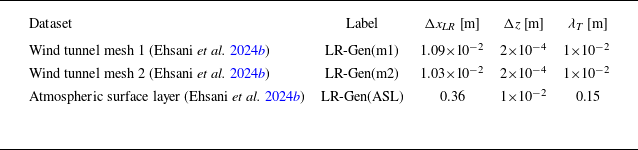
 λT
 ν
 τ
 uτ
 δ
 s
 0
 λT

 ρu,wVorX
 uVorX
 wVorX
 ρu,wVorX=−0.40

 z=2ks
 z<2ks
 z⩾2ks
 z<2ks
 z⩾2ks
 λT
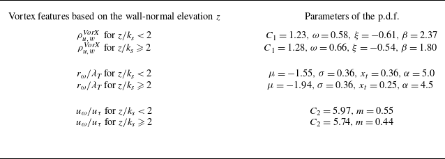
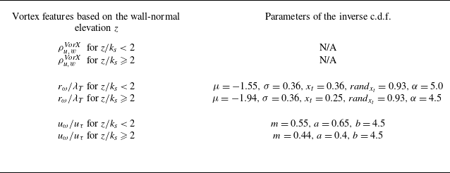

 |λci(x,z)|>γλci(r.m.s.)(z)
 |ωy(x,z)|>γωy(r.m.s.)(z)
 γ=0.35


 |λci(x,z)|>γλci(r.m.s.)(z)
 rω
 uω
 ρu,wVorX
 λci
 sgn(ωy)=+1
 2rω
 xcentroid
 λci
 sgn(ωy)=−1
 λci
 amax=2rω
 uHR-SGVF′>0
 randbinary∼B(0.5)=1

 uτ
 uconv+=8
 uconv+=11
 u+

 U¯/uτ=1/κln(z/z0)
 κ=0.39
 15⪅z/z0⪅30
 350⪅z/z0⪅600

 δ
 (u′u′¯/uτ2)=−Aln(z/δ)+B
 A=1.45
 B=1.57

 D11
 2A
 A
 k1−1

 z/δ=0.02
 z/δ=0.04

 z/δ=0.12
 z/δ=0.13

 z/δ=0.01
 z/δ=0.03

 λT2
 λT2


 Open access

