Brief overview of multiscale methods

The number of models developed at single scales is huge, ranging from density functional theory at the smallest scales, molecular dynamics at the atomic scale, and (semi-) discrete models, such as discrete dislocation plasticity, microstructural lattice models, continuum microstructural models, and continuum macroscopic models at larger and continuum scales. Each of these approaches aims to tackle the response of the considered material (or phase) at a given spatial scale and often also at a given temporal scale.

A microstructure, however, is a complex geometrical arrangement of different phases and interfaces. Linking the properties at the engineering scale (typically the scale of the device or component, which may range from micrometers to meters) to the microstructural scale inevitably requires a two-scale approach (or more, if needed). This is what characterizes a “multiscale” model.

Based on the nature and geometry of the scale of the heterogeneities, different types of multiscale methods can be distinguished. ^{Reference Engquist, Lao, Ren and Vanden-Eijnden9–Reference Fish12} Emphasis here is on spatial multiscale approaches seeking the effective macroscopic response of statistically representative volume elements (RVEs) of the underlying microstructure. The RVE is typically a sample volume element of material that is large enough to represent the statistical fluctuations in the microstructure and hence capture the effective (averaged) mechanical properties. From the perspective of the underlying problem formulation, one can distinguish between:

• • Concurrent methods—where both scales are simultaneously addressed, generally using different methodologies, for different scales, in different parts of the problem domain. ^{Reference Fish11}

• • Hierarchical methods—where different scales are hierarchically coupled in the same part of a domain (e.g., computational homogenization).

• • Hybrid methods—revealing a hybrid coupling scheme between the scales (e.g., generalized finite elements, ^{Reference Plews and Duarte13} quasi-continuum approach, ^{Reference Tadmor, Phillips and Ortiz14} multigrid methods, ^{Reference Miehe and Bayreuther15} and the variational multiscale method). ^{Reference Hughes, Feijoo, Mazzei and Quincy16}

The underlying solution procedure for each of the multiscale problems can be either (1) parallel (solving both scales monolithically), (2) serial or sequential (data passing between the scales), or (3) coupled or decoupled (using coupled online computations or decoupled offline computations).

The versatility of a multiscale method obviously depends on the assumptions made and the accuracy of the descriptions used at the underlying fine scales. Multiscale mechanics have evolved toward a methodology that naturally fills the gap within materials science, where the physics, synthesis, and material characterization of single phases and microstructures are a key concern. In the mechanics community, advanced nonlinear continuum models of detailed microstructures are being developed. In computational materials science, ^{Reference Raabe17,Reference Liu, Karpov, Zhang and Park18} various examples exist that unravel microscale mechanisms using analyses at the nanoscale (including Monte Carlo methods for statistical analyses). In this context, computational materials science and computational multiscale micromechanics have gradually started to merge.

Among the various multiscale methods developed, this article will touch upon one method in particular, computational homogenization, and also briefly report on some of the other methods. It should be noted that this mainly concerns the spatial multiscale problem. Many of the single-scale models make use of vastly different time scales (or loading rates), and incorporating them is possible if either no temporal scale transition is used (i.e., the fast microstructural fluctuations are fully resolved) or a time scale separation applies (i.e., fast fluctuations can be eliminated from the slow ones).

Computational homogenization

Homogenization of microstructures substitutes microstructural complexity by an equivalent homogeneous continuum. For this purpose, RVEs or representative unit cells are used.

In order to “homogenize” a microstructure, a scale separation principle must be adopted, implying that the relevant microscales are much smaller than the characteristic fluctuation scale in the macroscopic strain field. Many homogenization techniques have been developed, including composites, ^{Reference Agoras and Ponte Castañeda19} materials revealing size effects, ^{Reference Forest20} and random physically nonlinear materials. ^{Reference Ponte Castañeda21} Several asymptotic (or mathematical) homogenization approaches for nonlinear material behavior have been proposed and developed as well. ^{Reference Fish and Fan22}

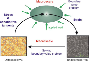
Computational homogenization is a powerful method to extract the macroscopic behavior on the basis of an underlying microstructural RVE. The method consists of a coupled solution of two nested boundary value problems, one at each scale. Figure 1 shows the elementary principles of the method for a mechanical homogenization problem. The deformation (strain) at the macroscopic scale is transferred to the microscale using deformation averaging, through which appropriate boundary conditions can be constructed. The solution of the microscale boundary value problem results in the macroscopic stress and tangent operators (derivatives of the stress tensor with respect to the strain or deformation tensor) using the energy consistency (Hill-Mandel) condition linking both scales. With the resulting macroscopic stress–strain behavior, a macroscale equilibrium problem can be solved (if needed).

Figure 1.

Computational homogenization is one of the most powerful methods to extract properties from a microstructure. (Top) The strain from the macroscale is passed to (bottom right) a representative volume element (RVE); (bottom, right to left) the microscale boundary value problem is solved; (bottom left) the average stress and constitutive tangents are extracted from the solution and passed (top) to the macroscale; the microscale problem shown here is a dual-phase steel loaded in 10% pure shear, solved with a fast Fourier-based solution technique. The deformed RVE highlights the equivalent plastic strain in the ferrite matrix phase.

If the finite element method (FEM) is used to solve the boundary value problems at both scales, the method is also referred to as the FE² method. ^{Reference Feyel and Chaboche23} The strength of this method is that it works for arbitrarily nonlinear behavior, including microstructural evolution at the microscale. The quality of the results depend on the modeling approximations made at the fine scale. There are no additional approximations at the coarse (macroscopic) scale. The basic (first-order) method is now well established. ^{Reference Zeman, de Geus, Vondrejc, Peerlings and Geers24–Reference Geers, Kouznetsova and Brekelmans28}

The computational homogenization scheme has been extended in various directions: higher-order continua ^{Reference Kouznetsova, Geers and Brekelmans29} (to address size effects); damage and localization; ^{Reference Bosco, Kouznetsova and Geers30} thermomechanics; ^{Reference Özdemir, Brekelmans and Geers31} substructured shells; ^{Reference Coenen, Kouznetsova and Geers32} cohesive interfaces; ^{Reference Matouš, Kulkarni and Geubelle33} electromagnetics; diffusion; sintering; heat flow, contact, and friction; ^{Reference Temizer34} and wave propagation in solids. ^{Reference Pham, Kouznetsova and Geers35} In terms of materials, applications can be found for metals, textiles, cellular and porous materials, composites, granular materials, soft matter, bone, and Li-ion batteries.

This method is powerful and accurate, and therefore, used often as a reference solution for other more simplified homogenization schemes. However, it comes with a high computational cost, which limits its applicability for many applications involving complex microstructures. To address this, appropriate algorithms have been developed to speed up multiscale simulations of this type, as discussed further in this article.

Copper-rubber interface delamination in stretchable electronics

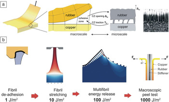
An example of the application of the computational homogenization method concerns the analysis of copper-rubber interfaces, used in most stretchable electronics applications. ^{Reference Vossen, van der Sluis, Schreurs, Geers, Neggers and Hoefnagels36–Reference Vossen, van der Sluis, Schreurs and Geers38} These interfaces typically fail as a result of rubber fibrillation at the rough copper interface (fibrils, attached to the copper, which are drawn from the rubber upon delamination). Even though the intrinsic microscale adhesion between copper and rubber polydimethylsiloxane is only in the range of 1 J/m², macroscopic peel tests report a work of separation of up to 1000 J/m² or more. Figure 2 illustrates the various contributions underlying this gap, ranging from fibril stretching, dynamical energy release in the fibrils and their bulk footings, and the interactions between neighboring fibrils.

Figure 2.

(a) Computational homogenization applied to a copper-rubber interface problem, from left to right: the delaminating interface at the macroscale; the macroscale cohesive zone (CZ) interfacial model, computing the traction vector (T _M) from the interfacial opening vector Δ _M; the microscale model with individual fibrils; and a micrograph of the real fibrils. (b) Energetic contributions to the macroscopic work of separation across the scales, from left to right: adhesion energy at the level of a single fibril; stretch energy of a fibril; energy release in the rubber upon fibril fracture or de-adhesion; and macroscopic work of separation in a peel test under an applied force F and an angle α. ^{Reference Vossen, Schreurs, van der Sluis and Geers37,Reference Vossen, van der Sluis, Schreurs and Geers38}

Advanced dislocation-based plasticity models

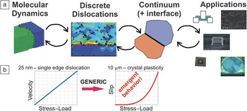
The plasticity of metals, ranging from the atomic scale via individual dislocations to collective dislocation motion toward macroscale plasticity, has been the subject of multiscale analysis for many years. ^{Reference Phillips1} Figure 3 illustrates the characteristic couplings between the scales. For metal plasticity, two recent structure–property modeling approaches are emphasized.

Figure 3.

Multiscale analysis of metals, from dislocations to crystal plasticity. (a) Scales and models involved, from left to right: atomistic scale, molecular dynamics; dislocation scale, discrete dislocation dynamics; single-crystal scale, crystal plasticity; application scale, continuum plasticity models. (b) (Left) The collective behavior of individual dislocations (linear velocity–stress profile) leads to (right) emergent contributions at the crystal continuum level (power-law slip–stress profile). ^{Reference Kooiman, Hütter and Geers42}

Kooiman et al. ^{Reference Kooiman, Hütter and Geers39–Reference Kooiman, Hütter and Geers42} analyzed the coarse graining of the collective behavior of dislocations using the general equation for the nonequilibrium reversible-irreversible coupling scheme. ^{Reference Öttinger43} One of the key results of this work, ^{Reference Kooiman, Hütter and Geers42} highlighted in Figure 3 (bottom plots), is that the macroscopic relation between applied mechanical load and dislocation flux is nonlinear (power law), whereas the input relation between load and dislocation velocity at the microscale is linear. This constitutes an emergent phenomenon, which is shown to be dominant over other contributions. Note that this method also properly handles the time-scale transition, ^{Reference Kooiman, Hütter and Geers42} which is one of the grand challenges in multiscale modeling.

The plasticity of metallic interfaces (e.g., grain and phase boundaries) is indicated in Figure 3 as well. This is a highly complex problem, since gliding dislocations interact with the grain-boundary defect structure, giving rise to dislocation pileups, dislocation absorption, transmission, and nucleation events. Van Beers et al. ^{Reference van Beers, McShane, Kouznetsova and Geers44–Reference van Beers, Kouznetsova and Geers47} proposed a thermodynamically consistent model for interface plasticity inspired by the results from atomistic simulations and discrete dislocation plasticity results. This model accounts for the grain-boundary energy and defect structure, as well the defect redistribution within the grain boundary upon absorbing dislocations in the grain boundary.

New methodologies for fast microstructural calculations on RVE

To model realistic microstructural RVEs in two dimensions ^{Reference Ambos, Willot, Jeulin and Trumel48} or three dimensions, efficient methods must be developed to reduce the costs related to fine-scale computations. Three-dimensional (3D) models are required in situations where two-dimensional (2D) models fall short, for example, for glass-fiber fibrous composites with nonparallel directions ^{Reference Altendorf, Jeulin and Willot49} or in complex morphologies, such as those encountered in cementitious ^{Reference Altendorf, Jeulin and Willot49} and polycrystalline materials. The main difficulty in taking complex 3D microstructural geometries into account is to define efficient high-resolution methods, especially when the microstructure is obtained from experimental microtomography images.

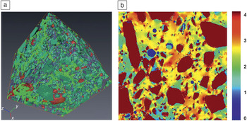
The fast Fourier transform (FFT) method ^{Reference Kouznetsova, Brekelmans and Baaijens26,Reference Moulinec and Suquet50–Reference Moulinec and Suquet52} is a fast numerical technique to solve the mechanical problem in the RVE. This image-based numerical method does not require prior meshing (finite element discretization), (i.e., partitioning the domain into simple geometrical subdomains), allowing handling of arbitrary (possibly evolving) microstructural geometries. Equilibrium and heat-flux conservation are, in particular, treated in the Fourier domain, assuming spatial periodicity of fields, even though the geometry is not itself periodic. Altendorf et al. ^{Reference Altendorf, Jeulin and Willot49} used FFT to study the local and effective properties of complex glass-fiber composites with high resolution. Escoda et al. ^{Reference Escoda, Willot, Jeulin, Sanahuja and Toulemonde53} used FFT to compute both local and effective stress fields in 3D high-resolution models (constructed from 3D gray-level images containing up to 735³ voxels) of mortar material microstructure (see Figure 4 ).

Figure 4.

(a) 3D view of a mortar microstructure, voids in red, aggregates in other colors, and transparent matrix. The displayed volume measures 1.25 × 1.25 × 1.25 cm³. (b) 2D section of the normalized mean stress component σ_m/[E _m〈ε〉] at high contrasts of elastic properties in the mortar microstructure of (a) loaded with an average volumetric strain 〈ε〉. σ_m, E _m denote the local hydrostatic stress and Young’s modulus, respectively. The resolution is 25 μm/voxel. Reproduced with permission from Reference Reference Escoda, Willot, Jeulin, Sanahuja and Toulemonde53. © 2011 Elsevier.

Lavergne et al. ^{Reference Lavergne, Sab, Sanahuja, Bornert and Toulemonde54} investigated the effect of the aggregate morphology on the viscoelastic effective behavior of concrete using FFT. Chen et al. ^{Reference Chen, Chen, Lebensohn, Ji, Heo, Bhattacharyya, Chang, Mathaudhu, Liu and Chen55} investigated the combined effects of mechanical loading and recrystallization in 3D polycrystals using combined FFT and phase-field modeling. Such studies allow the determination of the parameters in the microstructure that have an influence on the lifetime of the material. Yvonnet ^{Reference Yvonnet56} developed a modified FFT method operating in the real-space domain only, to avoid the alternate Fourier-space–real-space evaluation of the different operators and to facilitate parallelization.

A critical comparison between several methods for solving RVE problems with complex microstructures was provided in a recent review. ^{Reference Dunant, Bary, Giorla, Péniguel, Sanahuja, Toulemonde, Tran, Willot and Yvonnet57} Using a benchmark problem, classical discretization techniques, the eXtended Finite Element method ^{Reference Moës, Cloirec, Cartraud and Remacle58,Reference Tran, Yvonnet, He, Toulemonde and Sanahuja59} (for modeling interfaces in regular meshes), classical FEM with regular meshes and smoothed properties, ^{Reference Toulemonde, Masson and Gharib60} and the FFT methods were compared in terms of the resulting computational efficiency and accuracy. In particular, it was shown that the FFT method is the most efficient method for fine models in the absence of discontinuities such as cracks or imperfectly bounded interfaces, while the eXtended Finite Element method can provide an adequate accuracy even for coarse models by accurately describing the discontinuities at the interfaces.

Reducing computational costs in nonlinear coupled simulations at two scales

One of the main challenges of computational homogenization is the computational complexity involved in solving boundary value problems at two (or more) scales. Of particular interest are predictive multiscale methods, which include both the aforementioned realistic microstructures, and in addition, the macroscopic engineering scale with its loading conditions. These simulations can become extremely costly given the large number of degrees of freedom involved. Recent approaches aim to alleviate the computational complexity in two-scale simulations using parallel implementation strategies, reduced-order modeling, and decoupled approaches.

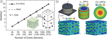
Parallelization of computational homogenization ^{Reference Feyel and Chaboche23,Reference Kouznetsova, Brekelmans and Baaijens26,Reference Geers, Kouznetsova and Brekelmans28} relies on the distribution of the numerous local microscale boundary value problems, typically evaluated at the integration points of the discretized macroscopic structure, over many processors (cores). Nguyen et al. ^{Reference Nguyen, Stroeven and Sluys61} introduced a parallel implementation of the FE² method for multiscale failure with multiphysics coupling for concrete. Ladevèze et al. ^{Reference Ladevèze, Loiseau and Dureisseix62} developed a domain-decomposition-like method to solve heterogeneous composite problems. In this context, the domain was decomposed into substructures and interfaces, and the so-called LATIN (Large Time INcrement) method was used to solve the two-scale problem. This technique involves a space–time decomposition of the fields in tandem with a special iterative solver involving a global linear problem and local nonlinear problems over the structure of interest. Fritzen et al. ^{Reference Fritzen, Hodapp and Leuschner63} proposed massively parallelizing FE² methods with graphical processing units. These specialized electronic circuits, originally designed to accelerate the display of images, were used to reduce the costs of multilevel techniques and gain several orders of magnitude computational cost reduction. Mosby and Matouš ^{Reference Mosby and Matouš64} developed massively parallel computing strategies to solve huge multiscale problems, the largest involving a total of 28.1 billion nonlinear equations solved on 393,216 computing cores. An example of their work is shown in Figure 5 .

Figure 5.

Computational speedup of a hierarchically parallel multiscale solver. (a) The macroscale is discretized with 17.5k finite elements and 9.8k nonlinear degrees of freedom (DOFs) and is computed using 32 cores. Each of the 512 representative unit cells (RUCs) are discretized with 1.46M finite elements and 773k nonlinear DOFs, and is computed using 512 cores. The complete multiscale simulation contains 747M finite elements and 396M DOFs. (b) (Bottom) The 1 and 2 strain plots are associated with the corresponding 1 and 2 points located on the (upper right) mid-plane of the structure. This figure illustrates the drastic computational time reduction enabled by parallel computations in nonlinear multiscale modeling. Reproduced with permission from Reference Reference Mosby and Matouš64. © 2016 IOP Publishing. Note: δ, applied displacement; σ_eq, equivalent stress; T _M, traction vector; e _eq, equivalent strain.

Introducing model reduction in FE² methods was first initiated for hyperelastic composites to study the effects of reinforcements in rubbers, ^{Reference Yvonnet and He65} where the proper orthogonal decomposition (POD) ^{Reference Lumley, Yaglom and Tataski66} technique was used to reduce local computations. POD is used for extracting correlations from arbitrary sets of data and determining the most relevant set of modes for an evolving system. These modes consist of linearly independent fields (e.g., displacement fields) that characterize the evolution of the system. Local computations were reduced by projecting local fields on a POD basis, then reducing the large sets of nonlinear equations of microstructural calculations. ^{Reference Yvonnet and He65}

Hernández et al. ^{Reference Hernández, Oliver, Huespe, Caicedo and Cante67} proposed a POD reduced-basis multiscale method with an interpolatory integration scheme that overcomes ill-posedeness problems (corresponding to nonuniqueness of the solution) in model reduction techniques of multiscale damage problems by embedding the gradient of the POD modes. Wen and Zabaras ^{Reference Wen and Zabaras68} proposed a POD multiscale method for stochastic FE² problems. Sparks and Oskay ^{Reference Sparks and Oskay69} proposed a method for identification of optimal reduced-order models for inelastic and failure response of heterogeneous materials, employing the eigendeformation-based reduced-order homogenization approach. Halabi et al. ^{Reference El Halabi, González, Chico and Doblaré70} recently replaced POD-parametrization of local fields in FE² by proper generalized decomposition ^{Reference Chinesta, Ammar and Cueto71} tensor product approximations to reduce costs related to offline computations.

Dvorak ^{Reference Dvorak72} initiated another important nonlinear micromechanical homogenization method, mainly applied to elasto-viscoplastic materials and metal-matrix composites, known as the transformation field analysis (TFA). In order to properly reproduce the local heterogeneous fields, nonuniform transformation analysis (NFTA) ^{Reference Michel and Suquet73,Reference Roussette, Michel and Suquet74} was developed. In this method, anelastic modes are extracted from snapshots of nonlinear simulations using POD. Fritzen et al. ^{Reference Fritzen and Sepe75} proposed an extended NTFA method and presented a comparative study between their method and NTFA, showing the limitations of classical NTFA and the more general character of their technique to handle arbitrary elasto-viscoplastic behaviors with rate dependency.

A last and promising class of methods is decoupled nonlinear homogenization methods. First a set of offline calculations is performed. Then, techniques are developed to construct “a posteriori” the effective behavior based on these calculations. Local calculations are no longer required, which reduces the cost of coupled multiscale simulations by several orders of magnitude. ^{Reference Yvonnet, Gonzalez and He76} A first natural choice is to identify functional forms of the macroscopic constitutive equations: ^{Reference Terada, Kato, Hirayama, Inugai and Yamamoto77} Numerical material tests are conducted on a unit cell to identify material parameters of the assumed constitutive law. This methodology implies “guessing” the form of the equation describing the effective behavior, which is not obvious in a general nonlinear context and for arbitrary (anisotropic) microstructures.

To overcome this issue, database methods were developed ^{Reference Terada, Kato, Hirayama, Inugai and Yamamoto77–Reference Klusemann and Ortiz80} to compute the response of nonlinear composites using an interpolation technique in a higher dimensional space from a prior set of databases composed of numerical evaluations of the quantities of interest (e.g., the effective energy of the RVE under various loads) computed from offline nonlinear calculations on the RVE. The obtained database can be compressed using tensor product approximations to accelerate macroscopic behavior evaluation during the structural (online) calculations. ^{Reference Yvonnet, Monteiro and He81} Such methods enabled the solution of one of the first nonlinear multiscale stochastic problems. ^{Reference Clement, Soize and Yvonnet82,Reference Clement, Soize and Yvonnet83} Another promising development is the use of neural networks in nonlinear multiscale methods ^{Reference Le, Yvonnet and He84} to construct fully decoupled approaches, where neural networks are employed to define the complex mapping between both macroscopic loading and microstructural parameters and the effective response of the RVE.