

Introduction
The influence of maternal birth month on reproductive performance has been addressed in various studies. Nonaka et al. (Reference Nonaka, Desjardins, Légaré, Charbonneau and Miura1990) found that in a sample of 17th and 18th century French-Canadians, women born between August and October had the lowest proportion of immediate conceptions after marriage, while those born between May and July achieved the highest. Smits et al. (Reference Smits, Van Poppel, Verduin, Jongbloet, Straatman and Zielhuis1997), based on a 19th century Dutch sample, concluded that nullipara displayed a birth distribution that was best represented by a bimodal curve with zeniths in January and July. A follow-up study confirmed two small temporal bands of reproductive failure, localized between January and February and July and August (Smits et al., Reference Smits, Jongbloet and Zielhuis2001). Lummaa & Tremblay (Reference Lummaa and Tremblay2003), utilizing 19th century Canadian family genealogies, showed that women born between November and March, and in June or September, had the highest number of grandchildren, whereas females born in April, July to August and October had the lowest reproductive success. Intriguingly, the birth month effect is not restricted to pre-modern societies. Based on data from the 2001 Austrian Microcensus, Huber et al. (Reference Huber, Fieder, Wallner, Moser and Arnold2004) documented that women born in the months of June to August had fewer live births, while women born in February to April and September had higher fertility counts (Jongbloet et al., Reference Jongbloet, Groenewoud, Huber, Fieder and Roeleveld2007). Huber and colleagues then extended their initial inquiry to address the influence of climato-geographical factors. Their results confirmed that the southern hemisphere displays a marked reversal of the European pattern (Huber et al., Reference Huber, Didham and Fieder2008), and that a tropical climate produces seasonal differentials that emulate those found in more temperate zones (Huber & Fieder, Reference Huber and Fieder2008).
From a biomedical perspective, there can be little doubt that human fertility is strongly shaped by environmental and genetic factors. But disparities in family formation can only be fully understood within the broader context of an individual's social institutions, experiences and relationships. Bongaarts (Reference Bongaarts1978) developed a comprehensive framework of these proximate fertility determinants that explains the inhibitive effects of various behavioural agents. For the question at hand, background, structural, societal and life-cycle factors have the highest explanatory power:
(a) Background factors. Aspects of the community of origin, such as the rural/urban divide. Aside from material conditions, rural population characteristics differ considerably from their urban counterpart. First, the occupational structure of rural areas is heavily skewed toward agriculture, a sector in which wages are often among the lowest. Second, rural areas are often characterized by persistent gender segregation. Operating in unison, these factors lead to early childbearing, either as a consequence of higher fertility norms or fewer career opportunities (Easterlin, Reference Easterlin1971).
(b) Structural conditions. Education and income further affect the timing and quantum of births due to their direct socioeconomic impact. Empirical data show that education imparts values, aspirations and skills that encourage and facilitate non-familial roles, independent of ethnic/national origin or cohort (d'Addio & d'Ercole, Reference d'Addio and d'Ercole2005). This is further compounded by the fact that lifetime-earnings differentials increase monotonically with education. Schooling – even before the advent of formal and obligatory education – is therefore tightly correlated with income, and inversely associated with birth count (Vinovskis, Reference Vinovskis1976). Within the economic theory of fertility, this interaction is stressed by the concept of ‘optimal parity’, which illustrates how parity progression is a direct function of all costs associated with raising a family, such as the net price of a child, the opportunity costs of a wife's time as well as various supply factors (Borg, Reference Borg1989).
(c) Societal factors. A large body of evidence suggests that shared cognitive beliefs or a common historical experience affect the timing of first and last birth. From a cross-cultural perspective, US Census results demonstrate that foreign-born females not only married at younger ages, but achieved higher percentages of complete nuptiality, an earlier onset of reproduction and higher parities at any given age (King & Ruggles, Reference King and Ruggles1990; Landale & Tolnay, Reference Landale and Tolnay1993; Morgan et al., Reference Morgan, Watkins, Ewbank and Watkins1994; Haines, Reference Haines1996). From a temporal perspective, cohorts develop and age, thus experiencing a unique segment of history. The most prominent temporal trend in Western fertility is, no doubt, the long-running decline in the quantum of births. While dating cultural change is inherently difficult, some reference points for the US population have emerged. Revised estimates of the crude birth rate suggest little or no change in fertility before 1840, with moderate decreases thereafter, primarily prompted by changes in nuptiality, including delays in age at first marriage and trends in permanent non-marriage (Haines, Reference Haines1996; Hacker, Reference Hacker2003).
(d) Aspects of the life cycle. Marital duration impacts on lifetime fertility. It has been widely observed that the number of children born within a union decreases with marital continuance, even when spousal age is controlled for (Henry, Reference Henry1980). This has been explained by changes in the coital frequency, which presents itself as non-monotonic trend (Jasso, Reference Jasso1985), but may also reflect changes in a couple's perception of ‘optimal parity’.
Formulation of the research question
The objective of the current study is to investigate the birth month effect, while controlling for several of the most common fertility predictors, such as birth cohort, husband's socioeconomic status (represented by Duncan's SEI), couple's urbanity, wife's nativity (as a proxy for ethnic origin and place of birth), wife's literacy (as a proxy for educational attainment) and duration of marital status. In order to detect covariate effects, the retrospective method was chosen, which – when based on a large sample – surveys lifetime reproductive outcome rather than relying on estimates. Although retrospective studies can be subject to potential biases in recruitment or recall, the benefits far outweigh the disadvantages. In order to overcome the problem of pregnancy-based data, census data were chosen that included information on nulliparity.
The birth month effect will be examined by contrasting two conventionally surveyed census variables: children ever born (CHBORN) and number of surviving children (CHSURV). The former provides a critical measure of lifetime fertility. The latter plays an important role in human behavioural ecology, as the number of surviving offspring is one of the most tractable measures commonly used to compare individual fitness or divergent reproductive strategies. Due to the nature of the data, both CHBORN as well as CHSURV are expressed as the total events incurred until the date of the enumeration. In order to gain proxies for completed fertility, inclusion in the sample pool was limited to post-reproductive women (≥45 years).
Methods
Data origin
Data were drawn from the Integrated Public Use Microdata Series (IPUMS), a collaborative project dedicated to the collection and distribution of census data and correlated documents (Ruggles et al., Reference Ruggles, Sobek, Alexander, Fitch, Goeken, Hall, King and Ronnander2008). The IPUMS database is a nationally representative high-precision series of census microdata files spanning the period from 1850 to 2000. All 1% historical census microdata samples employ the same basic sample design, with minor variations to accommodate differences in source materials and innovations in data-entry technology. In brief, within each enumeration district a random starting point between one and five is generated, and thereafter every fifth page is designated as a sample page. On each of these sample pages, sample points (i.e. households) are randomly selected. Therefore, the number of independent observations is the number of households, not the number of individuals. Unfortunately, clustering by household has implications for sample efficiency, as it increases the variance associated with most individual-level variables. For example, standard errors in cluster samples depend on both the size of the sampled clusters as well as on the variable homogeneity within these clusters. This loss of efficiency is effectively counterbalanced by stratification. By capitalizing on implicit categorization, the design yields high precision, especially for variables that are explicitly grouped, such as race, household size and group quarter status. In order to ensure an even geographical case distribution, samples for years prior to 1960 are based on regionally sorted source materials (Ruggles et al., Reference Ruggles, Sobek, Fitch, Hall and Ronnander1998).
Data preparation
The variable BIRTHMO reports the person's month of birth, but it is available only for persons under the age of one year for the census collections 1870, 1880 and 1950, and for all persons in 1900. Therefore, analyses had to be restricted to the Microdata Sample of the 1900 US Census. This subset is limited to a 1% nationally representative sample (760,081) of the total population (76,212,168).
The target variable BIRTHMO was available for 372,131 females, i.e. 49% of the total 1900 IPUMS. However, conjoint information on BIRTHMO and number of offspring or surviving children was only available for 167,026 women. Further reductions in sample size had to be accepted due to a selective but necessary sampling strategy that restricted all analyses to post-reproductive women, i.e. to females older than 45 years, in order to gain a proxy of completed fertility. An additional limitation was imposed by including only couples who were married for at least 10 years. Using the census codes AGE (age in years as of the last birthday) and BIRTHYR (person's year of birth) allowed for the construction of three cohorts to counter temporal trends in fertility and nuptiality. In cases where BIRTHYR conflicted with AGE, the individual was removed from further analyses. This left a total of 34,166 female records for observation of total fertility and 31,228 for child survival. The two subsets (CHBORN vs CHSURV) did not display any statistically significant differences in female birth cohort, birth year or birth month (Mann-Whitney test, p=0.419, p=0.399, p=0.855 respectively).
Measures of reproductive performance
Children ever born
(CHBORN) reports the number of children born to each woman. Females were to report all live births by all fathers, whether or not the children were still living. They were to exclude stillbirths, adopted children and stepchildren. For the purpose of the current study, if not otherwise stated, CHBORN includes individual reproductive output with a sample range of 0–25 births, and a mean of 5.5 births (SD=3.7). Surviving children (CHSURV) reports the number of children who were still living on census day. This includes all children born to a woman by all fathers, regardless of the child's current place of residence. Women were not to count adopted children or stepchildren. The sample range for CHSURV was 0–17, with a mean of 4.3 surviving offspring (SD=2.7).
Individual-level predictors
Maternal birth cohort
The census codes AGE (age in years as of the last birthday) and BIRTHYR (person's year of birth) were used to stratify the sample by cohort: 1826–1835 (n=3625; 10.6%), 1836–1845 (n=10482; 30.7%) and 1846–1855 (n=20059; 58.7%).
Husband's socioeconomic status (SES)
In IPUMS, each household's (i.e. husband's) socioeconomic status is represented by a constructed measure that assigns a Duncan Socioeconomic Index (SEI) score. This is a measure of occupational status based on the income level and educational attainment associated with each occupation in 1950. For modern samples, the range of observed SEI values typically falls between 1 and 97, with scores of 24 and 64 at the 1st and 3rd quartiles. Middle-class categories are associated with scores of between 35 and 65 (Duncan, Reference Duncan1961). For historical samples, a marked deviation from this trend is evident and expected. For the current subset, the household mean was 22.07 (SD=20.4), which emulates known census means for the period between 1850 and 1910 (Gardner, Reference Gardner2001).
Couple's urbanity
The census code URBAN indicates whether a household's location was urban or rural. While not without inherent problems, the term generally denotes all cities and incorporated places of 2500+ inhabitants (Ruggles et al., Reference Ruggles, Sobek, Alexander, Fitch, Goeken, Hall, King and Ronnander2008). All areas not classified as urban were designated as rural. Within the total sample, the vast majority were comprised of rural households (n=21,563; 63.1%), while the remainder were classified as urban (n=12,603; 36.9%).
Wife's nativity
This was used as a proxy for ethnic origin and place of birth. The census code NATIVITY indicates whether respondents were native- or foreign-born. For native-born individuals, a further differentiation includes parents' nativity. For the sample at hand, the original census designations were recoded based on a three-level scheme, which resulted in a subsample of native-born women (n=21,651; 63.4%), a subsample of native-born women with foreign-born parents ∼ 1st generation (n=3331; 9.7%) and a subsample of foreign-born women (n=9184; 26.9%).
Wife's literacy
The census code LIT indicates whether the respondent could read and/or write in any language, with separate indicators used for reading and writing. The four subgroups were recoded to reflect three responses, contrasting individuals who were illiterate (n=3666, 10.7%), with those who could read or write (n=728; 2.1%) and those who were fully literate (n=29,772, 87.1%). These literacy rates roughly reflect state variations in educational level (Vinovskis, Reference Vinovskis1976).
Duration of current marital status
This was based on the census variable DURMARR, which reports the number of years the respondent's current marital status had been in effect. The sample range was 10–66 years, with a mean of 30.4 years (SD=8.9). Duration of current marital status was re-grouped into 10-month bins, as this optimizes the display of structure in time-dependent data.
Statistical analyses
With the exception of time and seasonal trends, all statistical analyses were performed with SPSS 13. For the ANOVA procedure, only the variable ‘ID’ (a residual indexed by the person's ID number) required a log transformation to obtain normality. All models are based on separate analyses for CHBORN and CHSURV. In each model, CHBORN and CHSURV were used as dependent variables. Maternal month of birth as well as maternal birth cohort, couple's urbanity, wife's nativity and wife's literacy were fixed, while husband's socioeconomic status, duration of current marital status (10-month bins) and a residual error term were entered as covariates. All models were run to investigate both main and interaction effects. This yielded baseline values for CHBORN and CHSURV, with the influence of the other factors removed.
Temporal and seasonal trends were analysed with WinPEPI (Abramson, Reference Abramson2004), which provides procedures for the appraisal of seasonal variation. In the case of monthly data, the program routinely applies Freedman's and three other tests (Edwards's test, the ratchet circular scan test and Hewitt's test). As a default, the individual length of each month is taken into account. In addition, annual fertility data (parity and child survival) were checked for monthly variability and possible time trends using the non-parametric seasonal Mann-Kendall test.
Results
Socio-demographic sample profile
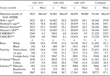
Table 1 summarizes the socio-demographic profile of the sample, stratified by cohort. With the exception of maternal month of birth (MMB) and nativity, cohort differences were evident for all variables under investigation. This is to be expected, as shifts in mean spousal age at enumeration, as well as marital duration, are a direct function of cohort grouping. By the same token, locality, literacy and husband's SES depict changes consistent with the impact of modernization and industrialization. For example, in younger cohorts, both the number of urban inhabitants and the husband's SES score increased, while the number of illiterates decreased. Table 1 also documents cohort-specific differences in the census statistic ‘race’. However, due to potential underenumeration biases (Condran, Reference Condran1984), race was omitted from further investigation.
Socio-demographic profile of the total sample, 1900 US Census (1% IPUMS), limited to post-reproductive women (age ≥45 years) and couples with a marital duration of ≥10 years (N=34,166)

* *Statistical significance at the 0.001 level. Significance levels denote cohort-specific differences.
a Peak month determined with Edward's test for a harmonic curve.
Time trends in lifetime fertility and child survival
As evident from Table 1, both CHBORN and CHSURV displayed statistically significant between-cohort differences. While these temporal changes mirror observations on the 19th century fertility transition and mimic the expected steady and long-term decline in infant and child mortality risk (Preston & Haines, Reference Preston and Haines1991; Haines, Reference Haines1998), time trends can act as a potential confounder. Thus, Mann-Kendall trend tests were applied to investigate the annual variation of both variables. Controlling for seasonal variation, the test did not detect a statistically significant trend in the number of children born (p=0.578) but verified a monotonic increase in offspring survival (p<0.001). Sen's estimator of slope indicated a median annual rise of 0.02 (95% CI=0.02 to 0.03). In order to control for maternal parity, the investigation was extended to include a survival ratio (CHBORN/CHSURV). As expected, the temporal trend persisted, albeit to a lesser degree (p<0.001, slope=−0.01, 95% CI=−0.01–−0.01).
Figure 1 displays the aggregated data for birth count and child survival across all maternal birth cohorts. A notable decline in the overall variation, as well as a pronounced cyclical pattern, is evident. Close inspection reveals seasonal peaks, nested around January to February, with troughs in mid-summer and autumn.
Reproductive performance (CHBORN, CHSURV) by maternal birth month across all cohorts. Values are expressed as raw scores, i.e. unadjusted for socio-demographic covariates. Mann-Kendall tests, controlling for seasonal variation, detected time trends in the number of surviving offspring (p<0.001, slope=0.02), but not in the total number of children born (p=0.578). Data source: 1900 US Census (1% IPUMS), limited to post-reproductive women (≥45 years) and couples with a marital duration ≥10 years (CHBORN N=34,166; CHSURV N=31,228).

Seasonal correlates
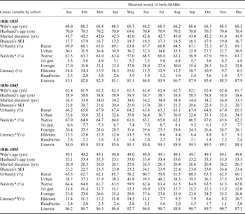
Monthly variations in the socio-demographic baseline characteristics were investigated to exclude potential seasonal biases. All analyses are based on the Ratchet Circular Scan test for a short seasonal peak, the results of which are summarized in Table 2. As is apparent, only few characteristics displayed a significant monthly variation. For all three cohorts, nativity showed slight but significant discrepancies in maternal birth season. This reflects a minute population-specific difference in the seasonal timing of births. Native-born women displayed a 3-month peak from January to March (28.6% of events; test statistic=13.31, p<0.005), while both first-generation and foreign-born females exhibited a seasonal peak from March to May (28.2% of events, test statistic=4.01, p<0.005; 30.7% of events, test statistic=12.09, p<0.005, respectively). Despite these subset-specific differences, the overall seasonal distribution mimicked the so-called ‘European pattern’ (spring peak with declining births for the rest of the year) rather than the expected ‘American pattern’, with its characteristic spring trough (Lam & Miron, Reference Lam and Miron1994). Intriguingly, the two younger cohorts also displayed a slight seasonal shift, from earlier towards later spring months, in the level of literacy (p<0.005). It is hypothesized that this could parallel educational attainment, as such differences have been noted elsewhere, and appear to be a function of birth month in relation to school year (Menet et al., Reference Menet, Eakin, Stuart and Rafferty2000).
Birth-month-specific differences between fertility covariates, stratified by cohort, 1900 US Census (1% IPUMS), limited to post-reproductive women (age ≥45 years) and couples with a marital duration of ≥10 years (N=34,166)

* *Statistical significance at the 0.001 level; *statistical significance at the 0.05 level.
The birth month effect
A multifactorial ANOVA was performed using SPSS GLM to assess whether total fertility (CHBORN) or subsequent child survival (CHSURV) can be predicted from maternal birth month after controlling for maternal cohort, husband's socioeconomic status, couple's urbanity, wife's nativity, wife's literacy and duration of current marital status. Preliminary data screening (testing for normal distribution and heteroscedasticity) indicated that the equality of variances assumption was violated (Levene test p<0.001). The failure to meet this criterion is not fatal to ANOVA. However, because the Levene test rejected homology of variances, the significance levels of all F-values were increased to p<0.001. In addition, all subsequent post-hoc analyses relied on tests not assuming unequal variances (Tamhane's T2).
In terms of variables that influenced CHBORN, significant main effects were observed for maternal month of birth (MMB) (F 11, 33606=1809.0, p<0.001), cohort(F 2, 33606=2393.8, p<0.001), literacy (F 2, 33606=455.4, p<0.001), urbanity (F 1, 33606=6528.4, p<0.001), nativity (F 2, 33606=8070.2, p<0.001) and duration of marriage (F 1, 33606=6000.4, p<0.001) but not for husband's SES (F 1,33606=0.190, p=0.663). Using partial eta squared (η 2) as the measure of association, MMB accounted for 37.2% of the total variability. This represents the highest value of η 2 – aside from nativity (32.4%), urbanity (16.3%) and marital duration (15.2%) – and suggests that MMB has high explanatory value. The corrected model (F 559, 33606=30999.8, p<0.001) was statistically significant and accounted for 99.8% of the total variability. In addition to main effects, a statistically significant interaction effect for total fertility (CHBORN) by maternal birth month, cohort, husband's socioeconomic status, couple's urbanity, wife's nativity, wife's literacy and duration of current marital status was observed (F 538, 33606=2.2, p<0.001). The corresponding effect size estimate was η 2=0.40.
The pattern of cell means indicated that women born in January (CHBORN=6.34, 95% CI=6.18–6.50), as well as September (6.34, 95% CI=6.17–6.51), February (6.33, 95% CI=6.17–6.49) and December (6.32, 95% CI=6.15–6.49), displayed above-average fertility counts, compared with females born during the remainder of the year (June 6.28, 95% CI=6.11–6.46; May 6.26, 95% CI=6.11–6.42; August 6.21, 95% CI=6.04–6.38). The lowest means were observed for women born in April (6.17, 95% CI=6.00–6.32), July (6.17, 95% CI=5.99–6.35), March (6.16, 95% CI=6.00–6.32), October (6.16, 95% CI=5.98–6.33) and November (6.14; 95% CI=5.97–6.32). Planned contrasts revealed that these differences achieved statistical significance (F 11, 31798=1712.9, p<0.001). Post-hoc multiple comparisons, assuming unequal variances, for cohort, literacy and nativity indicated that diachronic differences in fertility did not achieve statistical significance (1826–1835: 6.18, 95% CI=6.02–6.33; 1836–1845: 6.27, 95% CI=6.15–6.39; 1846–1855: 6.28, 95% CI=6.17–6.39), which supports previous assumptions that cohort effects were negligible. In contrast, fertility decreased with literacy status, which was expected (p>0.001). Literate females had on average 5.26 births (95% CI=5.19–5.32), which was substantially lower than the fertility counts of their contemporaries who could read or write (6.57, 95% CI=6.30–6.84) or who were completely illiterate (6.89, 95% CI=6.77–7.03). Similarly, differences in fertility between foreign-born females (6.88, 95% CI= 6.76–6.99) and native-born (5.78, 95% CI=5.61–5.89) or native-born with foreign-born parents (6.07, 95% CI=5.91–6.23) were evident, indicating that foreign-born females had higher fertility counts (p<0.001). Post-hoc tests could not be performed for urbanity, as there were fewer than three groups. But comparison of means indicated that women living in a rural environment had more children (5.79, 95% CI= 5.74–5.83) than city dwellers (4.95, 95% CI=4.88–5.01), which is in line with socio-demographic expectations.
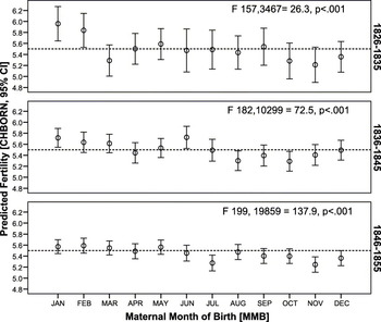
In a final step, separate cohort-specific ANOVAs were modelled to extract the predicted values for CHBORN, controlling for all factors of interest. The resultant data are plotted in Fig. 2. All models achieved statistical significance (1826–1835: F 157, 3467=26.3, p<0.001; 1836–1845: F 182, 10299=75.5, p<0.001; 1846–1855: F 199, 19859=137.9, p<0.001). Two observations emerge. First, from a seasonal perspective, the months of January, February, April and May are characterized by above-average fertility, while the lowest parity averages are found in mid-summer (July) and late autumn (October to November) to early winter (December). These fluctuations appear to be largely independent of cohort effects. Second, from a temporal perspective, seasonal peaks and troughs appear to be more pronounced for the earliest cohort, which could suggest a waning impact of the birth month effect across time.
Cohort-specific ANOVA models for predicted lifetime fertility by maternal birth month, controlling for all factors and covariates of interest (1826–1835: F 157, 3467=26.3, p<0.001; 1836–1845: F 182, 10299=75.5, p<0.001; 1846–1855: F 199, 19859=137.9, p<0.001). Data source: 1900 US Census (1% IPUMS), sample limited to post-reproductive women (age ≥45 years) and couples with a marital duration of ≥10 years (N=34,166).

Given that initial analyses had documented a meaningful and noticeable time trend on child survival, it was decided that further ANOVA exploration should only be warranted in the case of significant main effects for MMB. However, ANOVAs for child survival (number as well as ratio) indicated that main effects were either negligible (CHSURV: F 11, 30675=10.4, p<0.001, η 2=0.04) or failed to achieve statistical significance (ratio: F 11, 29646=1.346, p=0.192). Moreover, both models again indicated the presence of cohort effects (CHSURV F 2, 30675=351.9, p<0.001, η 2=0.22; ratio: F 2, 29646=129.4, p<0.001, η 2=0.09).
Discussion
The results of the current study confirm that family formation is the result of a well-defined number of biological and behavioural components, which serve to mediate the influence of culture, society, economic conditions, living standards and individual preferences. After removing the effect of various background, structural and societal influences on fertility progression, the current data suggest that having a birth month between January and May predisposes females to above-average fertility, while females born between July and December achieved only below-average offspring counts. The presented findings are in line with previous seasonal investigations (most notably, Huber et al. (Reference Huber, Fieder, Wallner, Moser and Arnold2004) and Jongbloet et al. (Reference Jongbloet, Groenewoud, Huber, Fieder and Roeleveld2007)), which likewise documented fertility peaks associated with the months February to April and marked troughs in the months June to August.
Intriguingly, the results also meet expectations from the seasonal optimal ripening oocyte (SOptRO) and seasonal preovulatory over-ripeness ovopathy (SPrOO) hypotheses (Jongbloet, Reference Jongbloet1992). The seasonal optimal ripening oocyte hypothesis predicts that optimal maturation of the oocyte, which coincides with the zenith of the ovulatory seasons, guarantees optimal realization and expression of the fetal genome and thus good progeny quality. The seasonal preovulatory over-ripeness ovopathy (SPrOO) hypothesis, on the other hand, posits that non-optimal maturation of the oocyte, which coincides with the transitional stages of the ovulatory pattern, as found during late autumn and early winter, compromises the expression of the fetal genome and results in pathologic conditions (Jongbloet et al., Reference Jongbloet, Groenewoud, Huber, Fieder and Roeleveld2007).
To elucidate the potential pathways for the birth month/fertility interaction, it is important to recognize that birth month is only a proxy for maternal season of conception. Thus, women with pronounced fertility were conceived in spring/early summer, while females with lower parity averages were conceived in late autumn/early winter. Classic Fetal Programming states that exogenous maternal malnutrition during pregnancy causes a persisting adaptation of the fetus resulting in long-term morbidity risks that extend well into adulthood (Barker, Reference Barker1998). The Advanced Fetal Programming Hypothesis proposes that maternal genes influence fetal well-being and induce an adaptation of the fetus (Hocher et al., Reference Hocher, Slowinski, Bauer and Halle2001). As the fetus adapts to a limited supply of nutrients, it permanently alters its physiology and metabolism, which inadvertently predisposes it to disease in later life, independent of the duration of gestation. Thus, perturbed fetal growth has been linked with an increased risk of coronary heart disease, diabetes, hypertension and stroke in adulthood (Osmond & Barker, Reference Osmond and Barker2000). On the plus side, this early adaptive response to environmental cues is evolutionary beneficial, as it enables short-term adaptations within one generation. On the downside, individuals developmentally adapted to one environment may be at risk when exposed to a different environment in later life (Bateson & Martin, Reference Bateson and Martin1999).
In the specific context of seasonality, it has often been observed that winter births run the highest risk for adverse health outcome due to increased exposure to infectious agents, pesticides, indoor environmental hydrocarbons or antihistamines. Other factors include the harmonic variation in population mixing, diet, temperature, humidity, sunlight/photoperiod, levels of vitamin D3 and endogenous hormones (Erfid & Nielsen, Reference Efird and Nielsen2008). The current finding that women born in late autumn (i.e. conceived in late winter) display below-average offspring counts, underscores the deleterious effects of cold temperature and nutritional deficiencies. However, an additional mechanism could operate through the differential distribution of Hp and ACP1 phenotypes. ACP1 has been shown to be associated with human fertility, congenital malformations, birth weight and intrauterine survival. Women homozygous for Hp with low ACP1 activity are more likely to conceive in the first part of the year, while women heterozygous for Hp with medium–high ACP1 activity are more likely to conceive in the latter part of the year. This suggests that ACP1 may play a role in delivering offspring into an environment favourable for development (Gloria-Bottini et al., Reference Gloria-Bottini, Bottini, La Torre, Magrini, Bergamaschi and Bottini2008). A concordant, highly significant association between ACP1 parameters and the season of conception can also be observed in newborn infants. ACP1 is controlled by a locus on chromosome 2 with three co-dominant alleles – *A, *B and *C – and there is evidence that infants conceived in January–April show an excess of the *A allele, which may signal an adaptation to colder climates (Gloria-Bottini et al., Reference Gloria-Bottini, Lucarini, Palmarino, La Torre, Amante and Bottini1997).
Recently, the Fetal Origins Hypothesis has been extended to account for differentials in female reproductive health, supporting the notion that women who have a genetic background allowing them to adapt easily to seasonal demands will be endowed with higher reproductive success (Davies & Norman, Reference Davies and Norman2002). Clinical evidence suggests that compromised prenatal growth is associated with a reduced ovarian fraction of primordial follicles (de Bruin et al., Reference de Bruin, Dorland, Bruinse, Spliet, Nikkels and Te Velde1998), a diminished ovarian and uterine volume at adolescence (Ibáñez et al., Reference Ibáñez, Potau, Enriquez and de Zegher2000), ovarian hyperandrogenism and anovulation in late adolescence (Ibáñez et al., Reference Ibáñez, Potau and de Zegher1999) as well as the timing of ovarian exhaustion (Cagnacci et al., Reference Cagnacci, Pansini, Bacchi-Modena, Giulini, Mollica, De Aloysio, Vadora and Volpe2005). For the question at hand, all these seasonally induced differentials have high explanatory power, particularly due to their potential impact on age at sexual maturation and age at menopause. However, at present, there is little proof that birth month directly affects the timing of menarche (Matchock et al., Reference Matchock, Susman and Brown2004). Month of birth and month of menarche appear to be largely unrelated, but there is some evidence that mean age at menarche is lower for girls born in November, December, May, June and July, and higher for those born in February, March, August, September and October, which indirectly suggests the existence of some seasonal mechanism (Boldsen, Reference Boldsen1992). Moreover, such seasonal fluctuations support the idea that a woman's birth month modulates her onset of fertility. Intriguingly, there is complementary socio-demographic evidence that shows that the timing of first marriage and childbearing are closely related to age at school graduation and thus, indirectly, to birth month. This implies that demographic events may underlie a relatively rigid sequencing, with age at school graduation emerging as an important factor in determining the timing – albeit not quantum – of family formation (Skirbekk et al., Reference Skirbekk, Kohler and Prskawetz2004). Aside from the onset of fertility, a woman's birth month has also been linked to fertility cessation. Clinical studies have determined that females born in autumn have a slightly higher reservoir of oocytes than females born in spring. This numerical difference appears to translate into minute but significant differences in the average age at menopause (spring born=49.4 years; autumn born= 49.9 years) (Cagnacci et al., Reference Cagnacci, Pansini, Bacchi-Modena, Giulini, Mollica, De Aloysio, Vadora and Volpe2005). However, in light of evidence that birth control measures have long been used to regulate family size, even before the onset of the fertility transition (Hacker, Reference Hacker2003), seasonally adjusted oocyte endowment by itself may have little explanatory power for fertility differentials.
The present study had initially set out to determine the impact of maternal birth month on offspring survivorship, but capitulated in light of emerging evidence that seasonal correlates may hold little explanatory power when cohort effects are considered. There is, however, evidence that child survival may be modulated by maternal birth month. Lummaa & Tremblay (Reference Lummaa and Tremblay2003) determined that women born between November and March, in June or September had more grandchildren than females born in April, July to August and October. While several of these key months coincide with the current study's seasonal pattern of higher and lower parity counts, clear methodological differences have to be acknowledged. Reproductive success is defined as the passing of genes on to the next generation, even though in practice it is often a tally of the number of offspring produced by an individual (Clutton-Brock, Reference Clutton-Brock1990). The number of progeny during an individual's lifetime is therefore an insufficient indicator of fitness, unless the number of offspring who attained reproductive age is taken into account. Census records, by their very nature, can only provide limited insights into the age structure of surviving offspring, as only those who reside with their natal family are considered. Moreover, census records only report the number of surviving children up to the point to enumeration, which cannot be equated to lifetime reproductive success. Aside from these deficits, trade-offs between offspring number and quality have to be considered. Evidence from family reconstitution suggests that variations in infant mortality may reflect differences in parental solicitude as a result of tensions generated between reproductive interests and ecological and economic constraints (Beise & Voland, Reference Beise and Voland2002). Therefore, the current finding that offspring survival was largely unaffected by maternal birth month, does not negate previous findings. Rather, it is hypothesized that the negligible effect of seasonal correlates needs to interpreted in the greater context of US mortality trends. Survival is the outcome of complex evolutionary mechanisms as well as the result of various social and demographic factors. The problem of finding causal associations is often compounded by regional as well as ethnic/racial divides. On the family level, income, wealth and literacy can play an important role. On the societal level, public health measures have to be considered. For the marked decline in US infant/child mortality during the 19th century, it appears that economic cycles have little explanatory power, while behavioural and environmental factors such as breast-feeding, childcare practices, hygiene and improvements in sanitation have emerged as primary drivers of these trends (Alter, Reference Alter, Bideau, Desjardins and Brignoli1997).
In summary, maternal birth month appears to be a strong component of female lifetime reproductive performance that can withstand controls for background, structural and societal predictors. Theoretically and practically grounded in the Fetal Origins Hypothesis, the association between maternal birth month and lifetime fertility extends fetal programming into the domain of female reproductive health.
Acknowledgments
The author would like to express profound gratitude to Ben P. Wise, PhD, for invaluable advice on statistical matters.