1 Introduction
The plasma periphery in a tokamak, extends from the external part of the closed flux surface region, typically referred to as the edge, to the scrape-off layer (SOL) region where the magnetic field lines intercept the machine vessel walls. These two regions are separated by the last closed flux surface (LCFS). Understanding the plasma dynamics in the periphery is necessary to address some the most crucial problems fusion is facing today, still undermining our capabilities to make reliable predictions of the performances of future tokamak, such as ITER (Shimada et al. Reference Shimada, Campbell, Mukhovatov, Fujiwara, Kirneva, Lackner, Nagami, Pustovitov, Uckan and Wesley2007). Indeed, the plasma dynamics in the periphery largely controls the plasma heat exhaust, the refuelling and helium removal. In addition, it governs the overall confinement performance of a tokamak. In fact, a low-to-high (L-H) confinement mode transition can be triggered if a heat power threshold is exceeded (Wagner Reference Wagner2007). This results from the formation of a transport barrier, which reduces considerably the turbulent transport, while a pressure pedestal appears in the proximity of the LCFS (Gohil et al. Reference Gohil, Burrell, Doyle, Groebner, Kim and Seraydarian1994). This barrier is characterized by strong radial electric fields yielding strong  $\boldsymbol{E}\times \boldsymbol{B}$ sheared flows (Burrell et al. Reference Burrell, Doyle, Gohil, Groebner, Kim, La Haye, Lao, Moyer, Osborne and Peebles1994; Schirmer et al. Reference Schirmer, Conway, Zohm and Suttrop2006; Xia, Shats & Punzmann Reference Xia, Shats and Punzmann2006), which are thought to be responsible for the observed reduction of the H-mode turbulence level (Petty et al. Reference Petty, Luce, DeBoo, Waltz, Baker and Wade1998; Naulin Reference Naulin2007). Once formed, the H-mode pedestal can periodically relax because of the presence of edge-localized modes (ELMs) releasing large amplitude bursts of particle and heat into the SOL (Zohm Reference Zohm1996; Connor & Wilson Reference Connor and Wilson2000; Kirk et al. Reference Kirk, Wilson, Akers, Conway, Counsell, Cowley, Dowling, Dudson, Field and Lott2005). ELM events are a major concern on the way to fusion energy.
The phenomena at play in the plasma periphery are mostly a consequence of the presence of electromagnetic fluctuations. These fluctuations determine the anomalous transport level (Stoneking et al. Reference Stoneking, Hokin, Prager, Fiksel, Ji and Den Hartog1994; Scott Reference Scott2003; LaBombard et al. Reference LaBombard, Hughes, Mossessian, Greenwald, Lipschultz and Terry2005; Snyder et al. Reference Snyder, Osborne, Burrell, Groebner, Leonard, Nazikian, Orlov, Schmitz, Wade and Wilson2012; Battaglia et al. Reference Battaglia, Burrell, Chang, Ku, DeGrassie and Grierson2014), the dynamics behind the L-H mode transition (Connor & Wilson Reference Connor and Wilson2000), they might have a role in the physics of the density limit (Rogers & Drake Reference Rogers and Drake1997; Rogers, Drake & Zeiler Reference Rogers, Drake and Zeiler1998; LaBombard et al. Reference LaBombard, Boivin, Greenwald, Hughes, Lipschultz, Mossessian, Pitcher, Terry and Zweben2001; Scott Reference Scott2003) and, furthermore, they are expected to limit the pedestal pressure gradient (Snyder et al. Reference Snyder, Groebner, Hughes, Osborne, Beurskens, Leonard, Wilson and Xu2011; Dickinson et al. Reference Dickinson, Roach, Saarelma, Scannell, Kirk and Wilson2012) and to set the SOL width (Scott Reference Scott1997; D’Ippolito, Myra & Krasheninnikov Reference D’Ippolito, Myra and Krasheninnikov2002; Scott Reference Scott2003; Halpern et al. Reference Halpern, Ricci, Jolliet, Loizu and Mosetto2014; Mosetto et al. Reference Mosetto, Halpern, Jolliet, Loizu and Ricci2015; Militello & Omotani Reference Militello and Omotani2016). Turbulent modes can develop into coherent filamentary structures with important perpendicular extension carrying a large amount of particles outwards in the SOL, strongly affecting the heat load on the plasma-facing components (Zweben et al. Reference Zweben, Boedo, Grulke, Hidalgo, LaBombard, Maqueda, Scarin and Terry2007; Agostini et al. Reference Agostini, Terry, Scarin and Zweben2011; Garcia, Horacek & Pitts Reference Garcia, Horacek and Pitts2015; Zweben et al. Reference Zweben, Davis, Kaye, Myra, Bell, Leblanc, Maqueda, Munsat, Sabbagh and Sechrest2015). These fluctuations occur on perpendicular scale lengths ranging from the particle Larmor radius,  $\unicode[STIX]{x1D70C}_{a}=v_{tha}/\unicode[STIX]{x1D6FA}_{a}$, to a scale length of the order of the typical equilibrium (in the sense of time-averaged) total pressure and potential gradient scale lengths, namely
 $L_{P}$ and
 $L_{\unicode[STIX]{x1D719}}$ (Ritz et al. Reference Ritz, Brower, Rhodes, Bengtson, Levinson, Luhmann, Peebles and Powers1987; Endler et al. Reference Endler, Niedermeyer, Giannone, Kolzhauer, Rudyj, Theimer and Tsois1995; LaBombard et al. Reference LaBombard, Boivin, Greenwald, Hughes, Lipschultz, Mossessian, Pitcher, Terry and Zweben2001; D’Ippolito et al. Reference D’Ippolito, Myra and Krasheninnikov2002; Garcia et al. Reference Garcia, Horacek, Pitts, Nielsen, Fundamenski, Naulin and Juul Rasmussen2007a; Nespoli et al. Reference Nespoli, Furno, Labit, Ricci, Avino, Halpern, Musil and Riva2017). Here,
 $a$ is the species subscript (i.e. for electrons
 $a=e$ and for the ions
 $a=i$),
 $v_{tha}^{2}=2T_{a}/m_{a}$ is the particle thermal velocity,
 $T_{a}$ is the particle temperature and
 $\unicode[STIX]{x1D6FA}_{a}=q_{a}B/m_{a}$ is the particle gyrofrequency, with
 $q_{a}$ and
 $m_{a}$ the particle charge and mass, respectively. The turbulent dynamics is thought to be the result of the complex nonlinear development of electromagnetic ion-temperature-gradient modes, drift waves, Kelvin–Helmholtz instabilities and ballooning modes (Scott Reference Scott1997; Zeiler et al. Reference Zeiler, Biskamp, Drake and Rogers1998; Rogers & Dorland Reference Rogers and Dorland2005; Mosetto et al. Reference Mosetto, Halpern, Jolliet, Loizu and Ricci2013). While these modes occur on the
 $\unicode[STIX]{x1D70C}_{i}$ and larger spatial scales (Mazzucato et al. Reference Mazzucato, Smith, Bell, Kaye, Hosea, Leblanc, Wilson, Ryan, Domier and Luhmann2008; Guttenfelder & Candy Reference Guttenfelder and Candy2011; Guttenfelder et al. Reference Guttenfelder, Peterson, Candy, Kaye, Ren, Bell, Hammett, LeBlanc, Mikkelsen and Nevins2013), there is evidence that also turbulent modes, occurring on the electron gyroscale with perpendicular wavenumber,
 $k_{\bot }$, satisfying
 $k_{\bot }\unicode[STIX]{x1D70C}_{e}\sim 1$, can contribute significantly to the large-scale heat flux and interact with modes at larger scales (Dorland et al. Reference Dorland, Jenko, Kotschenreuther and Rogers2000; Jenko et al. Reference Jenko, Dorland, Kotschenreuther and Rogers2000; Neiser et al. Reference Neiser, Jenko, Carter, Schmitz, Told, Merlo, Crandall, Mckee and Yan2018). Moreover, finite Larmor radius (FLR) effects might be important in the description of the pedestal (Snyder et al. Reference Snyder, Wilson, Ferron, Lao, Leonard, Osborne, Turnbull, Mossessian, Murakami and Xu2002). While the turbulent modes yield small amplitude fluctuations in the edge region (Brower, Peebles & Luhmann Reference Brower, Peebles and Luhmann1987; Ritz et al. Reference Ritz, Brower, Rhodes, Bengtson, Levinson, Luhmann, Peebles and Powers1987), order-unity fluctuation levels can be found in the SOL region with
 $k_{\bot }L_{P}\sim 1$ (Ritz et al. Reference Ritz, Brower, Rhodes, Bengtson, Levinson, Luhmann, Peebles and Powers1987; Wootton et al. Reference Wootton, Carreras, Matsumoto, McGuire, Peebles, Ritz, Terry and Zweben1990; Garcia et al. Reference Garcia, Pitts, Horacek, Madsen, Naulin, Nielsen and Rasmussen2007b; Xu et al. Reference Xu, Naulin, Fundamenski, Hidalgo, Alonso, Silva, Goncalves, Nielsen, Juul Rasmussen and Krasheninnikov2009; Zweben et al. Reference Zweben, Davis, Kaye, Myra, Bell, Leblanc, Maqueda, Munsat, Sabbagh and Sechrest2015; Nespoli et al. Reference Nespoli, Furno, Labit, Ricci, Avino, Halpern, Musil and Riva2017). In general, these turbulent modes display elongated structures in the direction parallel to the equilibrium magnetic field (Winslow et al. Reference Winslow, Bengtson, Richards and Craven1997; Zeiler et al. Reference Zeiler, Biskamp, Drake and Rogers1998; Thomsen et al. Reference Thomsen, Endler, Bleuel, Chankin, Erents and Matthews2002; Halpern et al. Reference Halpern, Jolliet, Loizu, Mosetto and Ricci2013; Grulke et al. Reference Grulke, Terry, Cziegler, Labombard and Garcia2014), and have typical frequencies considerably smaller than
 $\unicode[STIX]{x1D6FA}_{i}$ (Levinson et al. Reference Levinson, Beall, Powers and Bengtson1984; Ritz et al. Reference Ritz, Brower, Rhodes, Bengtson, Levinson, Luhmann, Peebles and Powers1987; Zweben et al. Reference Zweben, Boedo, Grulke, Hidalgo, LaBombard, Maqueda, Scarin and Terry2007).
Over the last decades, successful and significant progress has allowed important advances in the simulation of the turbulent plasma dynamics in the periphery. Both fluid (Dudson et al. Reference Dudson, Umansky, Xu, Snyder and Wilson2009; Tamain et al. Reference Tamain, Ghendrih, Tsitrone, Sarazin, Garbet, Grandgirard, Gunn, Serre, Ciraolo and Chiavassa2009; Ricci et al. Reference Ricci, Halpern, Jolliet, Loizu, Mosetto, Fasoli, Furno and Theiler2012; Easy et al. Reference Easy, Militello, Omotani, Dudson, Havlíĉková, Tamain, Naulin and Nielsen2014; Ricci Reference Ricci2015; Halpern et al. Reference Halpern, Ricci, Jolliet, Loizu, Morales, Mosetto, Musil, Riva, Tran and Wersal2016; Paruta et al. Reference Paruta, Ricci, Fiva, Wersal, Beadle and Frei2018) and gyrokinetic simulations (Xu et al. Reference Xu, Xiong, Dorr, Hittinger, Bodi, Candy, Cohen, Cohen, Colella and Kerbel2007; Cohen & Xu Reference Cohen and Xu2008; Ku, Chang & Diamond Reference Ku, Chang and Diamond2009; Shi, Hakim & Hammett Reference Shi, Hakim and Hammett2015; Hakim et al. Reference Hakim, Shi, Abel and Hammett2016; Pan, Told & Jenko Reference Pan, Told and Jenko2016; Chang et al. Reference Chang, Ku, Tynan, Hager, Churchill, Cziegler, Greenwald, Hubbard and Hughes2017; Pan et al. Reference Pan, Told, Shi, Hammett and Jenko2018) have been used to achieve this goal. Fluid models are usually based on the drift-reduced Braginskii equations (Braginskii Reference Braginskii1965; Zeiler, Drake & Rogers Reference Zeiler, Drake and Rogers1997; Simakov & Catto Reference Simakov and Catto2005; Scott Reference Scott2007), which evolve the three lowest-order fluid moments of the kinetic equation, that are the particle density, velocity and temperature. These fluid equations rely on high plasma collisionality as the fluid closure assumes that the particle distribution function is locally close to thermal equilibrium, and on the assumption that the perpendicular scale length of the fluctuations is large compared to  $\unicode[STIX]{x1D70C}_{i}$ (Hazeltine Reference Hazeltine1973; Zeiler et al. Reference Zeiler, Drake and Rogers1997; Catto & Simakov Reference Catto and Simakov2004). The assumption of local thermal equilibrium is hard to justify in the edge while it appears more reasonable in the SOL, where the particle temperatures are lower than in the core and at the top of the pedestal (Kocan et al. Reference Kocan, Gunn, Pascal, Bonhomme, Fenzi, Gauthier and Segui2008). However, significant deviations from thermal equilibrium can occur in the SOL. These deviations from a Maxwellian distribution function were numerically investigated by kinetic simulations (Lönnroth et al. Reference Lönnroth, Bateman, Bécoulet, Beyer, Corrigan, Figarella, Fundamenski, Garcia, Garbet and Huysmans2006; Tskhakaya Reference Tskhakaya2012; Battaglia et al. Reference Battaglia, Burrell, Chang, Ku, DeGrassie and Grierson2014), and are due to the presence of a tail of suprathermal particles, yielding important modifications to the parallel heat flux, transient processes (e.g. ELM bursts influencing locally the particle collisionality) and the sheath (Batishcheva et al. Reference Batishcheva, Batishchev, Shoucri, Krasheninnikov, Catto, Shkarofsky and Sigmar1996; Sigmar et al. Reference Sigmar, Batishcheva, Batishchev, Krasheninnikov and Catto1996; Batishchev et al. Reference Batishchev, Krasheninnikov, Catto, Batishcheva, Sigmar, Xu, Byers, Rognlien, Cohen and Shoucri1997; Kirk et al. Reference Kirk, Wilson, Akers, Conway, Counsell, Cowley, Dowling, Dudson, Field and Lott2005). These effects might be enhanced in typical ITER operating H-mode scenarios (Martin & Takizuka Reference Martin and Takizuka2008). To include kinetic modifications covering a different range of collisional regimes in a fluid description and non-Maxwellian physics, an extension of fluid models based on higher-order moments has been recently addressed by Jorge, Ricci & Loureiro (Reference Jorge, Ricci and Loureiro2017) within a drift-kinetic regime. This model considers potentially large electrostatic fluctuations by truncating an expansion of the electrostatic potential around the guiding-centre position, i.e. the centre of the particle gyration. Therefore, it is not able to properly describe fluctuations that occur on the particle gyroscale. Such fluctuations are particularly important in the description of anomalous transport in the edge region (Scott Reference Scott2003).
To describe fluctuations on the ion Larmor radius scale, gyrokinetic theories – pioneered by Catto (Reference Catto1978), Frieman & Chen (Reference Frieman and Chen1982) – were successfully used in numerical and theoretical investigations of microturbulences (Furnish et al. Reference Furnish, Horton, Kishimoto, LeBrun and Tajima1999; Heikkinen et al. Reference Heikkinen, Henriksson, Janhunen, Kiviniemi and Ogando2006; Brizard & Hahm Reference Brizard and Hahm2007; Idomura et al. Reference Idomura, Urano, Aiba and Tokuda2009; Wang & Hahm Reference Wang and Hahm2010; Hatch et al. Reference Hatch, Terry, Jenko, Merz and Nevins2011; Krommes Reference Krommes2012). Most of the gyrokinetic models are derived within the standard gyrokinetic ordering (Dubin, Krommes & Oberman Reference Dubin, Krommes and Oberman1983; Hahm Reference Hahm1988; Parra & Calvo Reference Parra and Calvo2014), i.e.
 $$\begin{eqnarray}\frac{\unicode[STIX]{x1D714}}{\unicode[STIX]{x1D6FA}_{i}}\sim \frac{e\unicode[STIX]{x1D719}_{1}}{T_{e}}\sim \frac{k_{\Vert }}{k_{\bot }}\ll 1,\end{eqnarray}$$
and
 $$\begin{eqnarray}k_{\bot }\unicode[STIX]{x1D70C}_{i}\sim 1,\end{eqnarray}$$
where  $\unicode[STIX]{x1D719}_{1}$ is the small amplitude fluctuating component of the electrostatic potential
 $\unicode[STIX]{x1D719}$, and
 $e=-q_{e}$. While allowing for
 $k_{\bot }\unicode[STIX]{x1D70C}_{i}\sim 1$ and being appropriate for core plasma conditions, the ordering given in (1.1) breaks down in the presence of large scale and amplitude fluctuations, such as the ones present in the SOL. The analytical treatment of large scale and amplitude electromagnetic fluctuations was addressed by Dimits, LoDestro & Dubin (Reference Dimits, LoDestro and Dubin1992) in a generalized gyrokinetic ordering, assuming that
 $k_{\bot }\unicode[STIX]{x1D70C}_{i}e(\unicode[STIX]{x1D719}-v_{\Vert }A_{\Vert })/T_{e}\ll 1$ where
 $A_{\Vert }$ is the parallel component of the fluctuating magnetic vector potential. This ordering is less restrictive than (1.1). Indeed, it allows for order-unity fluctuations,
 $e\unicode[STIX]{x1D719}/T_{e}\sim 1$, on long scale lengths
 $k_{\bot }\unicode[STIX]{x1D70C}_{i}\ll 1$, but also for
 $e\unicode[STIX]{x1D719}/T_{e}\ll 1$ on
 $k_{\bot }\unicode[STIX]{x1D70C}_{i}\sim 1$ scales. Gyrokinetic theories have also been developed to retain the presence of strong
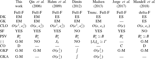
 $\boldsymbol{E}\times \boldsymbol{B}$ flows driven by large radial sheared electric fields in the internal and edge transport barrier regions (see, e.g. Bernstein & Catto Reference Bernstein and Catto1985; Brizard Reference Brizard1995; Hahm Reference Hahm1996; Hahm, Wang & Madsen Reference Hahm, Wang and Madsen2009; Dimits Reference Dimits2012). However, despite significant progress, the present gyrokinetic formulations do not provide yet an efficient framework for the description of the turbulent plasma periphery dynamics. The limitations of the present models are due to the lack of a proper description of arbitrarily far from equilibrium distribution functions in the presence of both large and small scale fluctuating electromagnetic fields and to the lack of a nonlinear gyrokinetic collision operator in a form that allows for an efficient numerical implementation, overcoming the extreme computational resources needed for the present edge gyrokinetic codes (Chang et al. Reference Chang, Ku, Tynan, Hager, Churchill, Cziegler, Greenwald, Hubbard and Hughes2017; Pan et al. Reference Pan, Told, Shi, Hammett and Jenko2018). In this regard, we note that gyrofluid models were developed to limit the computational cost of gyrokinetic simulations while overcoming the limitations of fluid models. These models aim to incorporate FLR and kinetic effects in a fluid-based description by taking a finite number of moments of the gyrokinetic equation (see, e.g. Brizard Reference Brizard1992; Dorland & Hammett Reference Dorland and Hammett1993; Waltz, Kerbel & Milovich Reference Waltz, Kerbel and Milovich1994; Beer & Hammett Reference Beer and Hammett1996; Snyder & Hammett Reference Snyder and Hammett2001; Ribeiro & Scott Reference Ribeiro and Scott2008; Madsen Reference Madsen2013; Held et al. Reference Held, Wiesenberger, Madsen and Kendl2016). The truncation schemes for closing the fluid models including collisionless Landau damping and perpendicular coupling between moments of the distribution function (associated with parallel streaming, magnetic gradient drifts and FLR effects) are usually obtained by techniques pioneered by Hammett & Perkins (Reference Hammett and Perkins1990), Hammett, Dorland & Perkins (Reference Hammett, Dorland and Perkins1992) and Dorland & Hammett (Reference Dorland and Hammett1993) and by methods developed by Waltz et al. (Reference Waltz, Kerbel and Milovich1994) and Beer & Hammett (Reference Beer and Hammett1996). Unfortunately, the limitations of these closure schemes undermine the use of gyrofluid models to evolve the plasma periphery dynamics due to the wide range of collisionality and the possible large deviations from equilibrium. Recently, an extension of the gyrofluid model to an arbitrary number of moments has been obtained by Mandell, Dorland & Landreman (Reference Mandell, Dorland and Landreman2018) in an Hermite–Laguerre pseudo-spectral velocity formulation of delta-F gyrokinetic theory for electrostatic perturbations in core conditions. This model allows for a dynamical refinement of previous gyrofluid models with a tuneable accuracy, and provides an ideal framework to approach the development of a gyrokinetic model for the plasma periphery.
In the present paper, leveraging previous works (Hammett et al. Reference Hammett, Beer, Dorland, Cowley and Smith1993; Beer & Hammett Reference Beer and Hammett1996; Sugama Reference Sugama2000; Hahm et al. Reference Hahm, Wang and Madsen2009; Zocco & Schekochihin Reference Zocco and Schekochihin2011; Madsen Reference Madsen2013; Omotani et al. Reference Omotani, Dudson, Havlìĉková and Umansky2015; Zocco et al. Reference Zocco, Loureiro, Dickinson, Numata and Roach2015; Loureiro et al. Reference Loureiro, Dorland, Fazendeiro, Kanekar, Mallet, Vilelas and Zocco2016; Schekochihin et al. Reference Schekochihin, Parker, Highcock and Dellar2016; Jorge et al. Reference Jorge, Ricci and Loureiro2017; Mandell et al. Reference Mandell, Dorland and Landreman2018), we derive a gyrokinetic model that we develop into a gyrokinetic moment (gyro-moment) hierarchy able to evolve the turbulent dynamics of the plasma in the periphery of tokamak devices. Our model allows us to describe far from equilibrium distribution functions, linear and nonlinear FLR effects driven by small-scale electromagnetic fluctuations and effects associated with time-dependent background electromagnetic fields in the presence of a strong sheared radial electric field. To construct our model, we introduce the small expansion parameters  $\unicode[STIX]{x1D716}=\unicode[STIX]{x1D70C}_{s}/L_{P}\ll 1$ and
 $\unicode[STIX]{x1D716}_{\unicode[STIX]{x1D6FF}}=e\unicode[STIX]{x1D719}_{1}/T_{e}\ll 1$, with
 $\unicode[STIX]{x1D70C}_{s}=c_{s}/\unicode[STIX]{x1D6FA}_{i}$ the sound Larmor radius and
 $c_{s}^{2}=T_{e}/m_{i}$ the sound speed. Collisional effects are treated by assuming the plasma strongly magnetized, and by introducing the small parameter
 $\unicode[STIX]{x1D716}_{\unicode[STIX]{x1D708}}=\unicode[STIX]{x1D708}_{i}/\unicode[STIX]{x1D6FA}_{i}\ll 1$ with
 $\unicode[STIX]{x1D708}_{i}\equiv \unicode[STIX]{x1D708}_{ii}$ the ion–ion collision frequency. The evolution equation of the distribution function, that is the gyrokinetic Boltzmann equation, is then obtained from fully nonlinear electromagnetic gyrokinetic equations of motion that are second-order accurate in
 $\unicode[STIX]{x1D716}$ and
 $\unicode[STIX]{x1D716}_{\unicode[STIX]{x1D6FF}}$. These equations are derived within a perturbation theory known as Lie-transform perturbation theory, pioneered by Littlejohn (Reference Littlejohn1982) and Cary & Littlejohn (Reference Cary and Littlejohn1983). Within this formulation, two successive non-canonical phase-space coordinates transformations are performed to decouple and remove the gyrophase-dependent part of the single particle motion from the slow drifts. We expand the full gyroaveraged distribution function onto a complete set of velocity-space Hermite–Laguerre polynomials. Projecting the gyrokinetic Boltzmann equation onto the Hermite–Laguerre basis yields an infinite set of coupled fluid equations describing the evolution of the expansion coefficients, termed gyro-moments. Collisional effects are introduced in our model by a nonlinear gyrokinetic Dougherty collision operator (Dougherty Reference Dougherty1964; Abel et al. Reference Abel, Barnes, Cowley, Dorland and Schekochihin2008). Finally, the gyro-moment hierarchy is coupled to a set of gyrokinetic Maxwell equations derived self-consistently from a gyrokinetic variational principle. This set includes two coupled gyrokinetic Poisson equations and two coupled gyrokinetic Ampere laws. Within this framework, polarization and magnetization effects appear from the phase-space coordinate transformations carried out in the single particle dynamics. These polarization and magnetization terms are expressed as functions of gyro-moments, yielding complete and closed analytical expressions of the gyrokinetic Maxwell equations.
The rest of the paper is organized as follows. In § 2, we order the main spatial and temporal scales at play in the plasma periphery and the relative amplitude of the electromagnetic fluctuations. In § 3, we describe the single particle dynamics by deriving a set of second-order accurate nonlinear electromagnetic gyrokinetic equations of motion by performing two phase-space coordinate transformations. In § 4, we derive the gyrokinetic Boltzmann equation. The expansion of the distribution function into a Hermite–Laguerre polynomial basis and the derivation of the gyro-moment hierarchy is presented in § 5, while the nonlinear gyrokinetic Dougherty collision operator is obtained and expanded in gyro-moments in § 6. Then, the gyro-moment hierarchy is self-consistently coupled to a set of gyrokinetic Maxwell equations deduced from a gyrokinetic variational principle in § 7. Finally, our main results are outlined in § 8. In particular, the improvements over previous gyrokinetic theories are summarized.
2 Ordering assumptions for the plasma periphery
In this section, we order the main spatial and temporal scales at play in the plasma periphery of tokamak devices. We first consider the scale lengths of the time-averaged profiles. We define the time-averaged perpendicular scale lengths of the total pressure  $P=\sum _{a}n_{a}T_{a}$, with
 $n_{a}$ and
 $T_{a}$ the density and temperature of species
 $a$, and of the electrostatic potential
 $\unicode[STIX]{x1D719}$, namely
 $L_{P}$ and
 $L_{\unicode[STIX]{x1D719}}$, as
 $L_{P}\sim |\unicode[STIX]{x1D735}_{\bot }\ln \langle P\rangle _{\unicode[STIX]{x1D70F}}|^{-1}$ and
 $L_{\unicode[STIX]{x1D719}}\sim |\unicode[STIX]{x1D735}_{\bot }\ln \langle \unicode[STIX]{x1D719}\rangle _{\unicode[STIX]{x1D70F}}|^{-1}$, with
 $\unicode[STIX]{x1D735}_{\bot }$ the gradient in the direction perpendicular to the magnetic field. The time-average operator,
 $\langle \cdot \rangle _{\unicode[STIX]{x1D70F}}$, acts over a time
 $\unicode[STIX]{x1D70F}$ such that
 $\unicode[STIX]{x1D70F}\unicode[STIX]{x1D714}\gg 1$, where
 $\unicode[STIX]{x1D714}$ is the typical frequency of the fluctuations, as defined by
 $\unicode[STIX]{x1D714}\sim |\unicode[STIX]{x2202}_{t}\ln n_{a}|\sim |\unicode[STIX]{x2202}_{t}\ln T_{a}|\sim |\unicode[STIX]{x2202}_{t}\ln \unicode[STIX]{x1D719}|$.
The definitions of  $L_{P}$ and
 $L_{\unicode[STIX]{x1D719}}$ allow us to introduce the small parameter
 $\unicode[STIX]{x1D716}$ as the ratio of the ion sound Larmor radius
 $\unicode[STIX]{x1D70C}_{s}$ to the equilibrium total pressure scale length
 $L_{P}$ (Frieman & Chen Reference Frieman and Chen1982),
 $$\begin{eqnarray}\unicode[STIX]{x1D716}=\frac{\unicode[STIX]{x1D70C}_{s}}{L_{P}}\sim \frac{\unicode[STIX]{x1D70C}_{s}}{L_{\unicode[STIX]{x1D719}}}\ll 1,\end{eqnarray}$$
where  $L_{P}\sim L_{\unicode[STIX]{x1D719}}$. We remark that
 $\unicode[STIX]{x1D70C}_{s}\sim \unicode[STIX]{x1D70C}_{i}$, whereas
 $\unicode[STIX]{x1D70C}_{i}/\unicode[STIX]{x1D70C}_{e}\sim \sqrt{m_{i}/m_{e}}\simeq 60$ for a deuterium plasma, assuming
 $T_{i}/T_{e}\sim 1$. Indeed,
 $1\lesssim T_{i}/T_{e}\lesssim 4$ in the plasma periphery (Kocan et al. Reference Kocan, Gunn, Pascal, Bonhomme, Fenzi, Gauthier and Segui2008; Elmore et al. Reference Elmore, Allan, Kirk, Fishpool, Harrison, Tamain, Kočan, Gaffka, Stephen and Bradley2012). While an alternative small parameter,
 $\unicode[STIX]{x1D70C}_{i}/L_{P}\ll 1$, can also be proposed (instead of
 $\unicode[STIX]{x1D70C}_{s}$ in (2.1)), the presence of turbulent modes in the plasma periphery with turbulent frequency
 $\unicode[STIX]{x1D714}/\unicode[STIX]{x1D6FA}_{i}\sim \unicode[STIX]{x1D70C}_{s}/L_{P}$ (Mosetto et al. Reference Mosetto, Halpern, Jolliet, Loizu and Ricci2013), that persist in the cold ion limit, motivates the definition in (2.1).
The spatial ordering in (2.1) is justified in many tokamaks and a wide range of experimental conditions. For example, in the edge region of the TEXT tokamak with plasma parameters  $B=2~\text{T}$,
 $I_{p}=200$ kA,
 $n_{e}\simeq 3\times 10^{19}~\text{m}^{-3}$, equilibrium scale lengths
 $L_{n}\sim L_{T_{e}}\sim L_{T_{i}}\sim L_{P}\sim 1.5~\text{cm}$ and
 $\unicode[STIX]{x1D70C}_{s}\sim \unicode[STIX]{x1D70C}_{i}\simeq 0.02~\text{cm}$, one has
 $\unicode[STIX]{x1D716}\sim 0.0167$ (Ritz et al. Reference Ritz, Brower, Rhodes, Bengtson, Levinson, Luhmann, Peebles and Powers1987). For a medium size tokamak, such as TCV, with
 $B=1.5~\text{T}$,
 $T_{e}\sim T_{i}\sim 40~\text{eV}$ and
 $n_{e}\simeq 6\times 10^{18}~\text{m}^{3}$, it is possible to estimate
 $\unicode[STIX]{x1D716}\sim 0.043$ (Rossel et al. Reference Rossel, Moret, Coda, Sauter, Goodman, Felici, Testa and Martin2012; Halpern et al. Reference Halpern, Ricci, Jolliet, Loizu, Morales, Mosetto, Musil, Riva, Tran and Wersal2016). For the edge transport barrier, typical values of
 $\unicode[STIX]{x1D716}\sim 1/30$ can be found in H-mode discharges in the JT60-U tokamak (Gohil et al. Reference Gohil, Burrell, Doyle, Groebner, Kim and Seraydarian1994). Additionally, equation (2.1) is also in agreement with detailed experimental measurements of the pedestal equilibrium scale lengths and scaling investigations of the H-mode pedestal structure (Burrell et al. Reference Burrell, Doyle, Gohil, Groebner, Kim, La Haye, Lao, Moyer, Osborne and Peebles1994; Hubbard Reference Hubbard2000; Wagner Reference Wagner2007; Zweben et al. Reference Zweben, Davis, Kaye, Myra, Bell, Leblanc, Maqueda, Munsat, Sabbagh and Sechrest2015). In general, in H-mode experimental conditions of large aspect ratio tokamaks, the equilibrium pedestal pressure scale length is often found to be of the order of the ion poloidal gyroradius,
 $\unicode[STIX]{x1D70C}_{\unicode[STIX]{x1D703}i}=\unicode[STIX]{x1D70C}_{i}B_{T}/B_{\unicode[STIX]{x1D703}}$ (where
 $B_{T}$ and
 $B_{\unicode[STIX]{x1D703}}$ are the toroidal and poloidal components of the equilibrium magnetic field, respectively) (Snyder et al. Reference Snyder, Aiba, Beurskens, Groebner, Horton, Hubbard, Hughes, Huysmans, Kamada and Kirk2009a), that is
 $L_{P}\sim \unicode[STIX]{x1D70C}_{\unicode[STIX]{x1D703}i}$, yielding
 $\unicode[STIX]{x1D716}\sim B_{\unicode[STIX]{x1D703}}/B_{T}\sim 1/10$. Although the latter estimate may break down in the edge of low aspect ratio devices such as MAST and NSTX (Ono et al. Reference Ono, Kaye, Peng, Barnes, Blanchard, Carter, Chrzanowski, Dudek, Ewig and Gates2000), the parameter
 $\unicode[STIX]{x1D716}$ remains small also in this kind of device (Kirk et al. Reference Kirk, Counsell, Arends, Meyer, Taylor, Valovic, Walsh and Wilson2004; Militello et al. Reference Militello, Tamain, Fundamenski, Kirk, Naulin and Nielsen2013). Finally, our ordering is valid in the operational conditions of ITER, as expected from predictions of its pedestal height and width (Snyder et al. Reference Snyder, Groebner, Leonard, Osborne and Wilson2009b; Beurskens et al. Reference Beurskens, Osborne, Schneider, Wolfrum, Frassinetti, Groebner, Lomas, Nunes, Saarelma and Scannell2011).
The equilibrium magnetic scale length  $L_{B}\sim |\unicode[STIX]{x1D735}_{\bot }\ln \hat{B}|^{-1}$ of the equilibrium magnetic field,
 $\hat{B}$, is ordered by the small parameter
 $$\begin{eqnarray}\unicode[STIX]{x1D716}_{B}=\frac{\unicode[STIX]{x1D70C}_{s}}{L_{B}}\sim \unicode[STIX]{x1D716}^{3}\end{eqnarray}$$
since  $L_{B}\sim R_{0}$, being
 $R_{0}$ the major radius of the tokamak device. We remark that, while one expects a maximal ordering
 $\unicode[STIX]{x1D716}_{B}\sim \unicode[STIX]{x1D716}$ for typical core conditions, in the plasma periphery where
 $L_{P}$ is steeper compared to the core, the scale length separation obeys
 $L_{P}/R_{0}<\unicode[STIX]{x1D70C}_{s}/L_{P}$ (Burrell et al. Reference Burrell, Doyle, Gohil, Groebner, Kim, La Haye, Lao, Moyer, Osborne and Peebles1994; Zweben et al. Reference Zweben, Boedo, Grulke, Hidalgo, LaBombard, Maqueda, Scarin and Terry2007) such that
 $\unicode[STIX]{x1D716}_{B}<\unicode[STIX]{x1D716}^{2}$, an assumption used in previous gyrokinetic edge model (see, e.g. Hahm et al. Reference Hahm, Wang and Madsen2009).
To describe the perpendicular scale length of the fluctuations, we introduce the perpendicular wavenumber,
 $$\begin{eqnarray}k_{\bot }\sim |\unicode[STIX]{x1D735}_{\bot }\ln n_{a}|\sim |\unicode[STIX]{x1D735}_{\bot }\ln T_{a}|\sim |\unicode[STIX]{x1D735}_{\bot }\ln P|\sim |\unicode[STIX]{x1D735}_{\bot }\ln \unicode[STIX]{x1D719}|,\end{eqnarray}$$
and the parameter
 $$\begin{eqnarray}\unicode[STIX]{x1D716}_{\bot }=k_{\bot }\unicode[STIX]{x1D70C}_{s}.\end{eqnarray}$$
Our model addresses the presence of turbulent fluctuations on scale lengths ranging from  $L_{P}$ to the
 $\unicode[STIX]{x1D70C}_{e}$ scale. More precisely, we consider large scale
 $\unicode[STIX]{x1D716}_{\bot }\sim \unicode[STIX]{x1D716}$ fluctuations, typically present in the SOL, where they appear with
 $k_{\bot }L_{P}\sim 1$, and may have large amplitude (Zweben et al. Reference Zweben, Davis, Kaye, Myra, Bell, Leblanc, Maqueda, Munsat, Sabbagh and Sechrest2015; Nespoli et al. Reference Nespoli, Furno, Labit, Ricci, Avino, Halpern, Musil and Riva2017). At the same time, we include
 $\unicode[STIX]{x1D716}_{\bot }\gtrsim 1$ fluctuations (Wootton et al. Reference Wootton, Carreras, Matsumoto, McGuire, Peebles, Ritz, Terry and Zweben1990; Shats, Xia & Punzmann Reference Shats, Xia and Punzmann2005). These fluctuations have scale length of the order of or smaller than
 $\unicode[STIX]{x1D70C}_{s}$, and include electron gyroscale fluctuations (
 $k_{\bot }\unicode[STIX]{x1D70C}_{e}\sim 1$), which are thought to be important in electron-temperature-gradient driven turbulent transport experiments (Dorland et al. Reference Dorland, Jenko, Kotschenreuther and Rogers2000; Colyer et al. Reference Colyer, Schekochihin, Parra, Roach, Barnes, Ghim and Dorland2017).
In order to describe the possible coexistence of electromagnetic fluctuations at amplitudes incompatible with the standard gyrokinetic ordering, in (1.1), and at scales ranging from the  $L_{P}$ scale to
 $\unicode[STIX]{x1D70C}_{s}$ (or smaller), we order the
 $\boldsymbol{E}\times \boldsymbol{B}$ drift,
 $\boldsymbol{u}_{E}=\boldsymbol{E}\times \boldsymbol{B}/B^{2}$, with
 $\boldsymbol{E}=-\unicode[STIX]{x1D735}\unicode[STIX]{x1D719}$, to be small with respect to the sound speed
 $c_{s}$, by introducing the parameter,
 $$\begin{eqnarray}\unicode[STIX]{x1D716}_{E}=\frac{|\boldsymbol{u}_{E}|}{c_{s}}\sim \unicode[STIX]{x1D716}_{\bot }\frac{e\unicode[STIX]{x1D719}}{T_{e}}\ll 1.\end{eqnarray}$$
The ordering in (2.5) allows for fluctuations of the order of the thermal energy on large scales, i.e.  $e\unicode[STIX]{x1D719}/T_{e}\sim 1$ for
 $\unicode[STIX]{x1D716}_{\bot }\sim \unicode[STIX]{x1D716}_{E}$ scales, and for small amplitude fluctuations, i.e.
 $e\unicode[STIX]{x1D719}/T_{e}\sim \unicode[STIX]{x1D716}_{E}$ for
 $\unicode[STIX]{x1D716}_{\bot }\sim 1$ scales. Also, it allows for the presence of fluctuations occurring at intermediate scales between
 $L_{P}$ and
 $\unicode[STIX]{x1D70C}_{s}$. While a sonic ordering,
 $\unicode[STIX]{x1D716}_{E}\sim 1$ yielding
 $e\unicode[STIX]{x1D719}/T_{e}\sim 1/\unicode[STIX]{x1D716}_{E}$ for
 $\unicode[STIX]{x1D716}_{\bot }\sim \unicode[STIX]{x1D716}_{E}$, has been considered in, e.g. Artun & Tang (Reference Artun and Tang1994), Brizard (Reference Brizard1995), Hahm (Reference Hahm1996) and Qin et al. (Reference Qin, Cohen, Nevins and Xu2007), here, we use the fact that fluctuations in the SOL satisfy
 $e\unicode[STIX]{x1D719}/T_{e}\sim 1$ on
 $\unicode[STIX]{x1D716}_{\bot }\sim \unicode[STIX]{x1D716}$ scales (Zweben et al. Reference Zweben, Davis, Kaye, Myra, Bell, Leblanc, Maqueda, Munsat, Sabbagh and Sechrest2015), while in the edge
 $e\unicode[STIX]{x1D719}/T_{e}\sim \unicode[STIX]{x1D716}_{\unicode[STIX]{x1D6FF}}\sim \unicode[STIX]{x1D716}$ on
 $\unicode[STIX]{x1D716}_{\bot }\sim 1$ scales (Brower et al. Reference Brower, Peebles and Luhmann1987), to find from (2.5) that the
 $\unicode[STIX]{x1D716}_{E}$ and
 $\unicode[STIX]{x1D716}$ parameters can have similar size.
The  $\boldsymbol{E}\times \boldsymbol{B}$ ordering in (2.5) is valid in both H- and L-mode, even when strongly equilibrium sheared radial electric fields and steep pressure gradients are present. In the L-H mode experimental conditions observed in the DIII-D tokamak, we observe
 $\boldsymbol{E}\times \boldsymbol{B}$ drift to the sound speed of the order of
 $|\boldsymbol{u}_{E}|/c_{s}\sim 1/10$, estimating
 $T_{i}\simeq 0.3~\text{KeV}$ and
 $B\simeq 2~\text{T}$ (Doyle et al. Reference Doyle, Groebner, Burrell, Gohil, Lehecka, Luhmann, Matsumoto, Osborne, Peebles and Philipona1991; Gohil et al. Reference Gohil, Burrell, Doyle, Groebner, Kim and Seraydarian1994). Similar values can be inferred from measurements of the long wavelength
 $\boldsymbol{E}\times \boldsymbol{B}$ flows in the edge of the HT-
 $7$ tokamak (Xu et al. Reference Xu, Wan, Song and Li2003). The ordering in (2.5) is also appropriate to describe the broadband turbulent power spectrum of the plasma periphery (Levinson et al. Reference Levinson, Beall, Powers and Bengtson1984; Ritz et al. Reference Ritz, Brower, Rhodes, Bengtson, Levinson, Luhmann, Peebles and Powers1987; Shats et al. Reference Shats, Xia and Punzmann2005) and the corresponding fluctuation levels. Indeed, the turbulent dynamics in the SOL is typically characterized by coherent filamentary structures with perpendicular gradient scale lengths
 $L_{P}\sim L_{\unicode[STIX]{x1D719}}$ (
 $k_{\bot }\unicode[STIX]{x1D70C}_{s}\sim 0.1$) and large amplitude fluctuations in the density and in the electrostatic potential, that are of the order of
 $T_{e}/e$, (Garcia et al. Reference Garcia, Horacek, Pitts, Nielsen, Fundamenski, Naulin and Juul Rasmussen2007a; Xu et al. Reference Xu, Naulin, Fundamenski, Hidalgo, Alonso, Silva, Goncalves, Nielsen, Juul Rasmussen and Krasheninnikov2009; Zweben et al. Reference Zweben, Davis, Kaye, Myra, Bell, Leblanc, Maqueda, Munsat, Sabbagh and Sechrest2015; Nespoli et al. Reference Nespoli, Furno, Labit, Ricci, Avino, Halpern, Musil and Riva2017). As observed in experimental characterizations of edge plasma turbulence (Ritz et al. Reference Ritz, Brower, Rhodes, Bengtson, Levinson, Luhmann, Peebles and Powers1987; Wootton et al. Reference Wootton, Carreras, Matsumoto, McGuire, Peebles, Ritz, Terry and Zweben1990; Fonck et al. Reference Fonck, Cosby, Durst, Paul, Bretz, Scott, Synakowski and Taylor1993; Wolf Reference Wolf2002; Wang et al. Reference Wang, He, Gao, Zeng, Zhang, Xie, Yang, Feng, Wang and Xiao2004; Xia et al. Reference Xia, Shats and Punzmann2006), the amplitude of these large fluctuations present in the SOL decreases inside the LCFS to residual levels, while the turbulent power spectrum in the edge peaks at
 $k_{\bot }\unicode[STIX]{x1D70C}_{i}\simeq 0.6$ with
 $\unicode[STIX]{x1D70C}_{i}\sim \unicode[STIX]{x1D70C}_{s}$ (Brower et al. Reference Brower, Peebles and Luhmann1987; Ritz et al. Reference Ritz, Brower, Rhodes, Bengtson, Levinson, Luhmann, Peebles and Powers1987). Thus, ion FLR effects might become non-negligible in this region (Snyder et al. Reference Snyder, Wilson, Ferron, Lao, Leonard, Osborne, Turnbull, Mossessian, Murakami and Xu2002; Dickinson et al. Reference Dickinson, Roach, Saarelma, Scannell, Kirk and Wilson2012). On the other hand, we remark that the particle parallel streaming velocity,
 $v_{\Vert }$, can be comparable to the sound speed. Values of the dimensionless parallel Mach number of the order of unity have been reported by experimental investigations of parallel flows (Wang et al. Reference Wang, He, Gao, Zeng, Zhang, Xie, Yang, Feng, Wang and Xiao2004; Pitts et al. Reference Pitts, Horacek, Fundamenski, Garcia, Nielsen, Wischmeier, Naulin and Juul Rasmussen2007).
For our model to allow for fluctuations at scales from  $L_{P}$ to
 $\unicode[STIX]{x1D70C}_{s}$, we separate the potential
 $\unicode[STIX]{x1D719}$ into two components, i.e. a drift-kinetic and a gyrokinetic component,
 $\unicode[STIX]{x1D719}_{0}$ and
 $\unicode[STIX]{x1D719}_{1}$, respectively (see § 3 for their rigorous definitions). Thus, we write (Dimits et al. Reference Dimits, LoDestro and Dubin1992)
 $$\begin{eqnarray}\unicode[STIX]{x1D719}=\unicode[STIX]{x1D719}_{0}+\unicode[STIX]{x1D719}_{1},\end{eqnarray}$$
and order the size of  $\unicode[STIX]{x1D719}_{1}$ to be small, at all scales from
 $L_{P}$ to
 $\unicode[STIX]{x1D70C}_{s}$, compared to the thermal energy by introducing the small parameter
 $$\begin{eqnarray}\unicode[STIX]{x1D716}_{\unicode[STIX]{x1D6FF}}=\frac{e\unicode[STIX]{x1D719}_{1}}{T_{e}}\ll 1.\end{eqnarray}$$
By imposing that both  $\unicode[STIX]{x1D719}_{0}$ and
 $\unicode[STIX]{x1D719}_{1}$ provide a similar contribution to
 $\boldsymbol{u}_{E}$, we order their gradients such that
 $|\unicode[STIX]{x1D735}_{\bot }\unicode[STIX]{x1D719}_{0}|\sim |\unicode[STIX]{x1D735}_{\bot }\unicode[STIX]{x1D719}_{1}|$. Equations (2.5) and (2.7) imply
 $|\unicode[STIX]{x1D70C}_{s}\unicode[STIX]{x1D735}_{\bot }\ln \unicode[STIX]{x1D719}_{1}|\sim 1$ such that
 $\unicode[STIX]{x1D719}_{1}$ is allowed to vary on all scales (from
 $L_{P}$ to
 $\unicode[STIX]{x1D70C}_{s}$), while
 $\unicode[STIX]{x1D719}_{0}$ is potentially large on large scale if
 $\unicode[STIX]{x1D716}_{\bot }\sim \unicode[STIX]{x1D716}$ (comparable to
 $L_{P}$) since
 $\unicode[STIX]{x1D716}_{\bot }e\unicode[STIX]{x1D719}_{0}/T_{e}\sim \unicode[STIX]{x1D716}_{E}\sim \unicode[STIX]{x1D716}$.
Following the critical balance conjecture (Goldreich & Sridhar Reference Goldreich and Sridhar1995; Schekochihin et al. Reference Schekochihin, Cowley, Dorland, Hammett, Howes, Plunk, Quataert and Tatsuno2008, Reference Schekochihin, Cowley, Dorland, Hammett, Howes, Quataert and Tatsuno2009, Reference Schekochihin, Parker, Highcock and Dellar2016), we order the parallel scale length  $k_{\Vert }\sim |\unicode[STIX]{x1D735}_{\Vert }\ln P|\sim |\unicode[STIX]{x1D735}_{\Vert }\ln \unicode[STIX]{x1D719}|$ by assuming that
 $c_{s}k_{\Vert }\sim k_{\bot }|\boldsymbol{u}_{E}|$ where
 $k_{\bot }|\boldsymbol{u}_{E}|$ is the frequency of the
 $\boldsymbol{E}\times \boldsymbol{B}$ flow. Following equation (2.5), this implies that
 $\unicode[STIX]{x1D70C}_{s}k_{\Vert }\sim \unicode[STIX]{x1D716}_{\bot }\unicode[STIX]{x1D716}$, i.e.
 $$\begin{eqnarray}\frac{k_{\Vert }}{k_{\bot }}\sim \unicode[STIX]{x1D716}.\end{eqnarray}$$
Equation (2.8) is compatible with experimental evidence of turbulent structures elongated in the parallel direction in the tokamak periphery and theoretical expectations of ballooning modes (Winslow et al. Reference Winslow, Bengtson, Richards and Craven1997; Bleuel et al. Reference Bleuel, Endler, Niedermeyer, Schubert and Thomsen2002; Naulin Reference Naulin2007; Garcia et al. Reference Garcia, Horacek, Pitts, Nielsen, Fundamenski, Naulin and Juul Rasmussen2007a; Halpern et al. Reference Halpern, Jolliet, Loizu, Mosetto and Ricci2013; Grulke et al. Reference Grulke, Terry, Cziegler, Labombard and Garcia2014). We remark that (2.2) and (2.8) imply that  $k_{\Vert }L_{B}\sim 1/\unicode[STIX]{x1D716}$ on the
 $L_{P}$ scales. This encompasses, e.g. ballooning mode structures for which the parallel wavenumber is of the order of the connection length, i.e.
 $L_{c}\simeq 2\unicode[STIX]{x03C0}qR_{0}$ with
 $R_{0}\sim L_{B}$ (Halpern et al. Reference Halpern, Jolliet, Loizu, Mosetto and Ricci2013), and drift wave turbulent modes which can be characterized by large
 $k_{\Vert }$ values (Rogers & Ricci Reference Rogers and Ricci2010; Mosetto et al. Reference Mosetto, Halpern, Jolliet, Loizu and Ricci2013).
The typical turbulent frequency  $\unicode[STIX]{x1D714}$ in the plasma periphery is much smaller than the ion gyrofrequency
 $\unicode[STIX]{x1D6FA}_{i}$. More precisely, we assume that the turbulent frequency is comparable to the frequency of the
 $\boldsymbol{E}\times \boldsymbol{B}$ flow, i.e.
 $\unicode[STIX]{x1D714}\sim k_{\bot }|\boldsymbol{u}_{E}|$ (Dimits Reference Dimits2012), yielding
 $$\begin{eqnarray}\frac{\unicode[STIX]{x1D714}}{\unicode[STIX]{x1D6FA}_{i}}\sim \unicode[STIX]{x1D716}_{\bot }\unicode[STIX]{x1D716},\end{eqnarray}$$
with  $\unicode[STIX]{x1D714}/\unicode[STIX]{x1D6FA}_{i}\sim \unicode[STIX]{x1D716}^{2}$ for large-scale fluctuations (Zeiler et al. Reference Zeiler, Drake and Rogers1997; Simakov & Catto Reference Simakov and Catto2005) while
 $\unicode[STIX]{x1D714}/\unicode[STIX]{x1D6FA}_{i}\sim \unicode[STIX]{x1D716}$ on the
 $\unicode[STIX]{x1D716}_{\bot }\sim 1$ scale length (Dubin et al. Reference Dubin, Krommes and Oberman1983; Hahm Reference Hahm1988; Hahm et al. Reference Hahm, Wang and Madsen2009). As a result of the orderings in (2.8) and (2.9), the parallel advection at the sound speed occurs on the same time scale as the turbulent fluctuations, i.e.
 $k_{\Vert }c_{s}\sim \unicode[STIX]{x1D714}$, in agreement with the critical balance that sets the parallel correlation length
 $L_{\Vert }\sim 1/k_{\Vert }$ of the perpendicular turbulent structure.
To describe magnetic fluctuations, we introduce a fluctuating magnetic vector potential  $\unicode[STIX]{x1D6FF}\boldsymbol{A}$. We assume that the fluctuating magnetic field,
 $\unicode[STIX]{x1D6FF}\boldsymbol{B}=\unicode[STIX]{x1D735}\times \unicode[STIX]{x1D6FF}\boldsymbol{A}$, is small compared to the large scale equilibrium magnetic field,
 $\hat{\boldsymbol{B}}=\unicode[STIX]{x1D735}\times \hat{\boldsymbol{A}}$, where
 $\hat{\boldsymbol{A}}$ is the magnetic vector potential associated with the large scale equilibrium magnetic field. More precisely, we impose
 $$\begin{eqnarray}\frac{|\unicode[STIX]{x1D6FF}\boldsymbol{B}|}{\hat{B}}\sim \unicode[STIX]{x1D716},\end{eqnarray}$$
with  $\hat{B}=|\hat{\boldsymbol{B}}|$, consistently with experimental measurements of edge magnetic fluctuations (Graessle, Prager & Dexter Reference Graessle, Prager and Dexter1991; Sötckel et al. Reference Sötckel, Badalec, Duran, Hron, Horacek, Jakubka, Kryska, Petrzilka, Zacek and Heller1999). We remark that both
 $\hat{\boldsymbol{B}}$ and
 $\hat{\boldsymbol{A}}$ vary on the
 $L_{B}$ scale, and that the temporal scale of
 $\hat{\boldsymbol{A}}$ is ordered as
 $$\begin{eqnarray}\frac{|\unicode[STIX]{x2202}_{t}\hat{\boldsymbol{A}}|}{c_{s}B}\sim \unicode[STIX]{x1D716}.\end{eqnarray}$$
This implies that  $\hat{\boldsymbol{B}}$ evolves on time scales such that
 $|\unicode[STIX]{x2202}_{t}\ln \hat{B}|/\unicode[STIX]{x1D6FA}_{i}\sim \unicode[STIX]{x1D716}\unicode[STIX]{x1D716}_{B}$ (Green et al. Reference Green2003; Hazeltine & Meiss Reference Hazeltine and Meiss2003; Wagner Reference Wagner2009). We remark that (2.11) allows us to retain the possible effects due to the change of the equilibrium magnetic field (e.g. for plasma shaping) that can occur on a time scale faster that the current diffusion time scale, but smaller that the typical frequency of the fluctuations. As a consequence of the ordering in (2.11), the inductive
 $\boldsymbol{E}\times \boldsymbol{B}$ velocity, i.e.
 $\boldsymbol{b}\times \unicode[STIX]{x2202}_{t}\hat{\boldsymbol{A}}/B$, remains small compared to
 $c_{s}$ (see (2.5)). The total fluctuating magnetic field can be written as
 $$\begin{eqnarray}\unicode[STIX]{x1D6FF}\boldsymbol{B}=\unicode[STIX]{x1D735}\times \unicode[STIX]{x1D6FF}\boldsymbol{A}_{\bot }+\unicode[STIX]{x1D735}\times (\unicode[STIX]{x1D6FF}A_{\Vert }\hat{\boldsymbol{b}}),\end{eqnarray}$$
where  $\unicode[STIX]{x1D6FF}A_{\Vert }\equiv \hat{\boldsymbol{b}}\boldsymbol{\cdot }\unicode[STIX]{x1D6FF}\boldsymbol{A}$ and
 $\unicode[STIX]{x1D6FF}\boldsymbol{A}_{\bot }\equiv \unicode[STIX]{x1D6FF}\boldsymbol{A}-\unicode[STIX]{x1D6FF}A_{\Vert }\hat{\boldsymbol{b}}$ are the parallel and perpendicular components of the fluctuating magnetic vector potential, respectively. Since compressional waves, associated with
 $\unicode[STIX]{x1D6FF}B_{\Vert }\equiv \hat{\boldsymbol{b}}\boldsymbol{\cdot }\unicode[STIX]{x1D6FF}\boldsymbol{B}$, are much faster than the typical turbulent time scale considered on the scales ranging from
 $L_{P}$ to
 $\unicode[STIX]{x1D70C}_{s}$ in low-
 $\unicode[STIX]{x1D6FD}$ plasmas (with
 $\unicode[STIX]{x1D6FD}=8\unicode[STIX]{x03C0}P/B^{2}$ the total thermal beta plasma) – as inferred from experimental measurements (Petty et al. Reference Petty, Luce, DeBoo, Waltz, Baker and Wade1998; Doyle et al. Reference Doyle, Houlberg, Kamada, Mukhovatov, Osborne, Polevoi, Bateman, Connor, Cordey and Fujita2007; Saibene et al. Reference Saibene, Oyama, Lönnroth, Andrew, De La Luna, Giroud, Huysmans, Kamada, Kempenaars and Loarte2007; Zweben et al. Reference Zweben, Boedo, Grulke, Hidalgo, LaBombard, Maqueda, Scarin and Terry2007) – we systematically neglect
 $\unicode[STIX]{x1D6FF}B_{\Vert }$. Thus, we describe
 $\unicode[STIX]{x1D6FF}\boldsymbol{B}_{\bot }$, at the lowest order, by a fluctuating magnetic vector potential along the equilibrium magnetic field, i.e.
 $$\begin{eqnarray}\unicode[STIX]{x1D6FF}\boldsymbol{B}=\unicode[STIX]{x1D6FF}\boldsymbol{B}_{\bot }\simeq \unicode[STIX]{x1D735}_{\bot }\unicode[STIX]{x1D6FF}A_{\Vert }\times \hat{\boldsymbol{b}},\end{eqnarray}$$
where we neglect the parallel component,  $\unicode[STIX]{x1D6FF}B_{\Vert }=\unicode[STIX]{x1D6FF}A_{\Vert }\hat{\boldsymbol{b}}\boldsymbol{\cdot }\unicode[STIX]{x1D735}\times \hat{\boldsymbol{b}}$ since it is of higher order and
 $\unicode[STIX]{x1D6FF}\boldsymbol{A}_{\bot }$. This removes completely the compressional Alfvén waves in our model. We remark that this approximation is consistent with low-
 $\unicode[STIX]{x1D6FD}$ plasma models currently implemented in global and edge gyrokinetic codes (see, e.g. Goerler et al. Reference Goerler, Lapillonne, Brunner, Dannert, Jenko, Merz and Told2011; Lanti et al. Reference Lanti, Ohana, Tronko, Hayward-Schneider, Bottino, McMillan, Mishchenko, Scheinberg, Biancalani and Angelino2019; Mandell et al. Reference Mandell, Hakim, Hammett and Francisquez2019), and fulfils the plasma periphery conditions. We also show that our low-
 $\unicode[STIX]{x1D6FD}$ approximation is in fact compatible with the presence of steep equilibrium pressure gradients in § 7.4. Finally, we deduce that
 $\unicode[STIX]{x1D719}\sim c_{s}\unicode[STIX]{x1D6FF}A_{\Vert }$ by comparing the
 $\boldsymbol{E}\times \boldsymbol{B}$ ordering in (2.5) with (2.10) (Brizard & Hahm Reference Brizard and Hahm2007; Dimits Reference Dimits2012; Tronko et al. Reference Tronko, Bottino, Chandre and Sonnendruecker2017a). This allows a general treatment of magnetic fluctuations in a maximal ordering.
Similarly to (2.6), the parallel component of the fluctuating magnetic potential,  $\unicode[STIX]{x1D6FF}A_{\Vert }$, can be written as
 $$\begin{eqnarray}\unicode[STIX]{x1D6FF}A_{\Vert }=A_{\Vert 0}+A_{\Vert 1},\end{eqnarray}$$
with  $A_{\Vert 0}$ and
 $A_{\Vert 1}$ the drift-kinetic and gyrokinetic parts of the fluctuating magnetic potential, respectively. The time variation of
 $A_{\Vert 0}$ and
 $A_{\Vert 1}$ obeys (2.9). By imposing that both
 $A_{\Vert 0}$ and
 $A_{\Vert 1}$ provide a similar contribution to
 $\unicode[STIX]{x1D6FF}\boldsymbol{B}_{\bot }$, we order
 $|\unicode[STIX]{x1D735}_{\bot }A_{\Vert 0}|\sim |\unicode[STIX]{x1D735}_{\bot }A_{\Vert 1}|$. In addition, the ordering given in (2.7) with
 $\unicode[STIX]{x1D719}_{1}\sim c_{s}A_{\Vert 1}$ yields
 $c_{s}eA_{\Vert 1}/T_{e}\sim \unicode[STIX]{x1D716}_{\unicode[STIX]{x1D6FF}}$ such that
 $A_{\Vert 1}$ is small at all scales, while
 $A_{\Vert 0}$ can be potentially large at large scales since
 $\unicode[STIX]{x1D716}_{\bot }ec_{s}A_{\Vert 0}/T_{e}\sim \unicode[STIX]{x1D716}_{E}$. Thus, the magnetic field from
 $A_{\Vert 0}$ and the large-scale component,
 $\hat{\boldsymbol{B}}$, is written as
 $$\begin{eqnarray}\boldsymbol{B}=\hat{\boldsymbol{B}}+\unicode[STIX]{x1D735}_{\bot }A_{\Vert 0}\times \hat{\boldsymbol{b}},\end{eqnarray}$$
while the magnetic field generated by the small amplitude component  $A_{\Vert 1}$ is
 $\boldsymbol{B}_{1}=\unicode[STIX]{x1D735}_{\bot }A_{\Vert 1}\times \hat{\boldsymbol{b}}$, as such, the total magnetic field is given by
 $\boldsymbol{B}+\boldsymbol{B}_{1}$. We also remark that (2.9) gives the ordering of the inductive part of the parallel electric field, with
 $\unicode[STIX]{x2202}_{t}A_{\Vert 0}\sim \unicode[STIX]{x1D716}^{2}\unicode[STIX]{x1D6FA}_{i}A_{\Vert 0}$ and
 $\unicode[STIX]{x2202}_{t}A_{\Vert 1}\sim \unicode[STIX]{x1D716}\unicode[STIX]{x1D6FA}_{i}A_{\Vert 1}$ yielding
 $$\begin{eqnarray}\frac{E_{\Vert }}{|\boldsymbol{E}_{\bot }|}\sim \unicode[STIX]{x1D716}.\end{eqnarray}$$
In order to describe the different collisional regimes in the plasma periphery, we introduce the small parameter  $\unicode[STIX]{x1D716}_{\unicode[STIX]{x1D708}}=\unicode[STIX]{x1D708}_{i}/\unicode[STIX]{x1D6FA}_{i}\ll 1$ where
 $\unicode[STIX]{x1D708}_{i}\equiv \unicode[STIX]{x1D708}_{ii}$ is the ion–ion collision frequency. By imposing that the plasma remains strongly magnetized, we require that
 $$\begin{eqnarray}\unicode[STIX]{x1D716}_{\unicode[STIX]{x1D708}}=\frac{\unicode[STIX]{x1D708}_{i}}{\unicode[STIX]{x1D6FA}_{i}}\sim \unicode[STIX]{x1D716}^{2}.\end{eqnarray}$$
From (2.17), the electron–electron collision frequency  $\unicode[STIX]{x1D708}_{e}\equiv \unicode[STIX]{x1D708}_{ee}$ is ordered as
 $$\begin{eqnarray}\frac{\unicode[STIX]{x1D708}_{e}}{\unicode[STIX]{x1D6FA}_{i}}\sim \sqrt{\frac{m_{i}}{m_{e}}}\left(\frac{T_{i}}{T_{e}}\right)^{3/2}\unicode[STIX]{x1D716}_{\unicode[STIX]{x1D708}},\end{eqnarray}$$
with  $\unicode[STIX]{x1D708}_{e}\sim \sqrt{m_{i}/m_{e}}(T_{i}/T_{e})^{3/2}\unicode[STIX]{x1D708}_{i}$. In order to estimate the level of collisionality in the plasma periphery, we look at the ratio of the electron mean-free path,
 $\unicode[STIX]{x1D706}_{mfp}=v_{the}/\unicode[STIX]{x1D708}_{e}$, to the parallel scale length
 $L_{\Vert }\sim 1/k_{\Vert }$. Equations (2.8) and (2.18) yield the estimate
 $$\begin{eqnarray}k_{\Vert }\unicode[STIX]{x1D706}_{mfp}\sim \frac{\unicode[STIX]{x1D716}\unicode[STIX]{x1D716}_{\bot }}{\unicode[STIX]{x1D716}_{\unicode[STIX]{x1D708}}}.\end{eqnarray}$$
From (2.19), one infers that our model is compatible with high ( $k_{\Vert }\unicode[STIX]{x1D706}_{mfp}<1$) and low (
 $k_{\Vert }\unicode[STIX]{x1D706}_{mfp}>1$) collisionality regimes.
The ordering given in (2.17) is compatible with experimental conditions. Indeed, with typical TCV SOL parameters, estimating  $B=1.4~\text{T}$,
 $n_{e}\simeq 1\times 10^{18}~\text{m}^{-3}$,
 $T_{e}\sim T_{i}\sim 25~\text{eV}$, one finds
 $\unicode[STIX]{x1D716}_{\unicode[STIX]{x1D708}}\simeq 0.0003$ (Garcia et al. Reference Garcia, Pitts, Horacek, Madsen, Naulin, Nielsen and Rasmussen2007b; Nespoli et al. Reference Nespoli, Furno, Labit, Ricci, Avino, Halpern, Musil and Riva2017), and for JET discharges, estimating the SOL parameters by
 $B=2.4~\text{T}$,
 $n_{e}\simeq 10^{18}~\text{m}^{-3}$ and
 $T_{e}\sim T_{i}\sim 40~\text{eV}$, one obtains
 $\unicode[STIX]{x1D716}_{\unicode[STIX]{x1D708}}\simeq 8.3\times 10^{-5}$ (Erents et al. Reference Erents, Chankin, Matthews and Stangeby2000; Xu et al. Reference Xu, Naulin, Fundamenski, Hidalgo, Alonso, Silva, Goncalves, Nielsen, Juul Rasmussen and Krasheninnikov2009). Lower values of
 $\unicode[STIX]{x1D716}_{\unicode[STIX]{x1D708}}$ are typical of the edge due the presence of ELMs, when temperatures are of the order of
 $T_{e}\sim T_{i}\sim 100~\text{eV}$, and
 $\unicode[STIX]{x1D716}_{\unicode[STIX]{x1D708}}\sim 10^{-6}$ (Pitts et al. Reference Pitts, Alberti, Blanchard, Horacek, Reimerdes and Stangeby2003; Kirk et al. Reference Kirk, Wilson, Akers, Conway, Counsell, Cowley, Dowling, Dudson, Field and Lott2005).
3 Single particle dynamics in the plasma periphery
Following previous gyrokinetic models (Dimits et al. Reference Dimits, LoDestro and Dubin1992; Qin et al. Reference Qin, Cohen, Nevins and Xu2006; Hahm et al. Reference Hahm, Wang and Madsen2009; Dimits Reference Dimits2012; Madsen Reference Madsen2013), we derive a model for the single particle dynamics in the plasma periphery by performing two successive changes of phase-space coordinates. Taking advantage of the low-frequency ordering in (2.9), these two transformations allow us to pass from the particle phase-space, described by the coordinates  $(\boldsymbol{x},\boldsymbol{v},t)$ where
 $\boldsymbol{x}$ is the particle position,
 $\boldsymbol{v}$ is the particle velocity measured in the laboratory reference frame and
 $t$ is the time coordinate, to a set of new coordinates where the fast gyromotion, associated with the gyrophase-dependent part of the particle motion, is decoupled and removed from the gyrophase-independent low-frequency (compared to
 $\unicode[STIX]{x1D6FA}_{a}$) drifts. In addition, the transformations ensure the adiabatic invariance of one phase-space coordinate. The transformations we perform are obtained by using Lie-transform perturbation theory, a class of continuous change of phase-space coordinates that preserve the Hamiltonian structure of the original system. We remark that, since the coordinate systems are connected by an invertible transformation, the physics is not affected by the use of the new coordinates (Qin & Tang Reference Qin and Tang2004).
The present section is organized as follows. In § 3.1, we describe the general methodology we follow to obtain the proper description of the single particle dynamics in the plasma periphery. The mathematical tools associated with Lie-transform perturbation theory are introduced in § 3.2. Then, the first and second phase-space coordinate transformations are presented in §§ 3.3 and 3.4, respectively.
3.1 General methodology
Within a coordinate-independent formulation, the dynamics of a particle of species  $a$ is prescribed by its action
 ${\mathcal{A}}_{a}=\int L_{a}\,\text{d}t=\int \unicode[STIX]{x1D6FE}_{a}$, where
 $L_{a}$ is the particle Lagrangian and
 $\unicode[STIX]{x1D6FE}_{a}=L_{a}\,\text{d}t$ is the Lagrangian one-form. In this section, we drop the particle subscript
 $a$ for simplicity. The Lagrangian one-form
 $\unicode[STIX]{x1D6FE}$ is given, in the
 $(6+1)$-dimensional particle phase-space described by the coordinates
 $\boldsymbol{z}=(\boldsymbol{x},\boldsymbol{v},t)$, by (Jackson Reference Jackson2012)
 $$\begin{eqnarray}\displaystyle \unicode[STIX]{x1D6FE} & = & \displaystyle [q\boldsymbol{A}+m\boldsymbol{v}]\boldsymbol{\cdot }\text{d}\boldsymbol{x}-\left[q\unicode[STIX]{x1D719}+\frac{mv^{2}}{2}\right]\,\text{d}t\nonumber\\ \displaystyle & \equiv & \displaystyle \unicode[STIX]{x1D738}\boldsymbol{\cdot }\text{d}\boldsymbol{z}=\unicode[STIX]{x1D6FE}_{\unicode[STIX]{x1D708}}\,\text{d}\boldsymbol{z}^{\unicode[STIX]{x1D708}},\end{eqnarray}$$
where we use the Einstein’s notation and we denote  $\boldsymbol{A}=\boldsymbol{A}(\boldsymbol{x},t)$ and
 $\unicode[STIX]{x1D719}=\unicode[STIX]{x1D719}(\boldsymbol{x},t)$ the magnetic vector potential and electrostatic potential evaluated at the particle position
 $\boldsymbol{x}$, and
 $\boldsymbol{z}^{\unicode[STIX]{x1D708}}$ is the
 $\unicode[STIX]{x1D708}$ component of
 $\boldsymbol{z}$. In general, the Greek index
 $\unicode[STIX]{x1D708}$ runs from
 $1$ to
 $6+1$ (since it includes the time coordinate
 $t$), whereas the Latin index
 $i$ runs from
 $1$ to
 $6$. Thus,
 $\boldsymbol{z}=(\boldsymbol{z}^{i},t)$ and
 $\unicode[STIX]{x1D738}=(\unicode[STIX]{x1D6EC}_{i},-{\mathcal{H}})$ with
 $\unicode[STIX]{x1D6EC}_{i}$ and
 ${\mathcal{H}}$ the symplectic and Hamiltonian components of the one-form
 $\unicode[STIX]{x1D6FE}$, respectively. In particular, in (3.1),
 $\unicode[STIX]{x1D6EC}_{i}=qA_{i}+mv_{i}$ for
 $i=1,2,3$ with
 $A_{i}$ the
 $i$th component of the magnetic vector potential
 $\boldsymbol{A}$, while
 $\unicode[STIX]{x1D6EC}_{i}=0$ for
 $i=4,5,6$ and
 ${\mathcal{H}}=q\unicode[STIX]{x1D719}+mv^{2}/2$.
To decouple the fast gyromotion from to the low-frequency drifts in the particle dynamics, both contained in  $\unicode[STIX]{x1D6FE}$, two successive changes of coordinates are performed from the particle phase space,
 $\boldsymbol{z}$. In the first coordinate transformation, we introduce the lowest-order guiding-centre coordinates,
 $\boldsymbol{Z}_{0}=(\boldsymbol{x}_{0},v_{\Vert 0},\unicode[STIX]{x1D707}_{0},\unicode[STIX]{x1D703}_{0},t)$. In this coordinate system,
 $\boldsymbol{x}_{0}$ is the zeroth-order guiding-centre position, i.e.
 $\boldsymbol{x}_{0}\equiv \boldsymbol{x}$ corresponds to the particle position, and the coordinates
 $(v_{\Vert 0},\unicode[STIX]{x1D707}_{0},\unicode[STIX]{x1D703}_{0})$ are introduced as a first step to decouple the gyrophase-dependent and -independent parts of the particle motion. In particular,
 $v_{\Vert 0}=\boldsymbol{v}\boldsymbol{\cdot }\boldsymbol{b}$ is the parallel velocity (
 $\boldsymbol{b}=\boldsymbol{B}/B$),
 $\unicode[STIX]{x1D703}_{0}$ is the lowest-order gyrophase angle and
 $\unicode[STIX]{x1D707}_{0}$ is the lowest-order magnetic moment. More precisely, the coordinates
 $\unicode[STIX]{x1D703}_{0}$ and
 $\unicode[STIX]{x1D707}_{0}$ are defined by introducing the right-handed Frenet–Serret orthonormal vector basis
 $(\boldsymbol{e}_{1},\boldsymbol{e}_{2},\boldsymbol{b})$ with
 $(\boldsymbol{e}_{1},\boldsymbol{e}_{2})$ spanning the plane perpendicular to
 $\boldsymbol{b}$ (Frenet Reference Frenet1852; Littlejohn Reference Littlejohn1988). We also introduce the associated cylindrical vector basis
 $(\boldsymbol{a},\boldsymbol{b},\boldsymbol{c})$, where
 $\boldsymbol{a}\equiv \boldsymbol{a}(\boldsymbol{x}_{0},\unicode[STIX]{x1D703}_{0},t)$ and
 $\boldsymbol{c}\equiv \boldsymbol{c}(\boldsymbol{x}_{0},\unicode[STIX]{x1D703}_{0},t)$ are defined with respect the coordinate angle
 $\unicode[STIX]{x1D703}_{0}$, i.e.
 $$\begin{eqnarray}\displaystyle & \displaystyle \boldsymbol{a}(\boldsymbol{x}_{0},\unicode[STIX]{x1D703}_{0},t)=\cos \unicode[STIX]{x1D703}_{0}\boldsymbol{e}_{1}(\boldsymbol{x}_{0},t)-\text{sin}\,\unicode[STIX]{x1D703}_{0}\boldsymbol{e}_{2}(\boldsymbol{x}_{0},t), & \displaystyle\end{eqnarray}$$
 $$\begin{eqnarray}\displaystyle & \displaystyle \boldsymbol{c}(\boldsymbol{x}_{0},\unicode[STIX]{x1D703}_{0},t)=-\text{sin}\,\unicode[STIX]{x1D703}_{0}\boldsymbol{e}_{1}(\boldsymbol{x}_{0},t)-\text{cos}\,\unicode[STIX]{x1D703}_{0}\boldsymbol{e}_{2}(\boldsymbol{x}_{0},t). & \displaystyle\end{eqnarray}$$
From (3.2) and (3.3), we remark that  $\boldsymbol{c}=\unicode[STIX]{x2202}_{\unicode[STIX]{x1D703}_{0}}\boldsymbol{a}$. The
 $\unicode[STIX]{x1D703}_{0}$ coordinate is then explicitly introduced by writing the particle velocity as
 $$\begin{eqnarray}\boldsymbol{v}=\boldsymbol{U}+\boldsymbol{c}_{\bot }^{\prime },\end{eqnarray}$$
with  $\boldsymbol{U}$ and
 $\boldsymbol{c}_{\bot }^{\prime }\equiv v_{\bot }\boldsymbol{c}$ being the gyrophase independent and dependent parts of the particle velocity, respectively (discussed more in the detail in § 3.3). Then,
 $v_{\bot }$, the perpendicular velocity measured in the frame moving with the velocity
 $\boldsymbol{U}$, is used to define the lowest-order adiabatic magnetic moment
 $\unicode[STIX]{x1D707}_{0}=mv_{\bot }^{2}/(2B)$. Given the velocity decomposition in (3.4), the gyrophase-dependent part of the velocity,
 $\boldsymbol{c}_{\bot }^{\prime }$, can be isolated in the particle one-form
 $\unicode[STIX]{x1D6FE}$ in (3.1). This allows us to perform a perturbative change of coordinates from the
 $\boldsymbol{Z}_{0}$ coordinates to the guiding-centre phase-space coordinates denoted by
 $\boldsymbol{Z}=(\boldsymbol{R},v_{\Vert },\unicode[STIX]{x1D707},\unicode[STIX]{x1D703},t)$. The guiding-centre coordinates,
 $\boldsymbol{Z}$, are constructed such that the dynamics is described by a gyrophase independent guiding-centre one-form
 $\unicode[STIX]{x1D6E4}=\unicode[STIX]{x1D6E4}(\boldsymbol{R},v_{\Vert },\unicode[STIX]{x1D707},t)$, removing the gyrophase terms associated with background gradients. As a consequence, the guiding-centre magnetic moment
 $\unicode[STIX]{x1D707}$ is dynamically conserved. We remark that the time coordinate
 $t$ does not change under the transformations. We perform this perturbative transformation up to second order in the small parameter
 $\unicode[STIX]{x1D716}$. We note that this is equivalent to carry out an expansion in the
 $m/q\sim \unicode[STIX]{x1D6FA}^{-1}$ parameter, considered in previous literature (Northrop Reference Northrop1963; Kruskal Reference Kruskal1965; Littlejohn Reference Littlejohn1979; Brizard Reference Brizard1995; Hazeltine & Meiss Reference Hazeltine and Meiss2003). Then, we order the terms with respect to the parameter
 $\unicode[STIX]{x1D716}_{E}$ (see (2.1)) up to second order to obtain a suitable guiding-centre model for the plasma periphery, considering potentially large amplitude electromagnetic fluctuations present on the
 $L_{P}$ scale length (Dimits Reference Dimits2012). We neglect the
 $\unicode[STIX]{x1D716}_{\unicode[STIX]{x1D6FF}}$ electromagnetic fluctuations in the guiding-centre transformation. The second-order accuracy is motivated by the importance of retaining the lowest-order FLR corrections and the effects associated with a time-dependent
 $\boldsymbol{E}\times \boldsymbol{B}$ drift.
The second perturbative change of coordinates is from the guiding-centre to the gyrocentre coordinates, denoted by  $\overline{\boldsymbol{Z}}=(\overline{\boldsymbol{R}},\overline{v}_{\Vert },\overline{\unicode[STIX]{x1D707}},\overline{\unicode[STIX]{x1D703}},t)$. Within this change of coordinates, we consider the presence of small-scale electromagnetic fluctuations,
 $\unicode[STIX]{x1D719}_{1}(\boldsymbol{x})$ and
 $A_{\Vert 1}(\boldsymbol{x})$, on the
 $\unicode[STIX]{x1D716}_{\bot }\sim 1$ scales, and perturb the guiding-centre one-form. The conservation of the guiding-centre adiabatic magnetic moment
 $\unicode[STIX]{x1D707}$, violated by the presence of the small scale fluctuations, is retrieved in the gyrocentre magnetic moment
 $\overline{\unicode[STIX]{x1D707}}$, up to second order in the small amplitude parameter
 $\unicode[STIX]{x1D716}_{\unicode[STIX]{x1D6FF}}$, by the perturbative construction of
 $\overline{\boldsymbol{Z}}$. As a result, we obtain the gyrophase-independent gyrocentre one-form
 $\overline{\unicode[STIX]{x1D6E4}}=\overline{\unicode[STIX]{x1D6E4}}(\overline{\boldsymbol{R}},\overline{v}_{\Vert },\overline{\unicode[STIX]{x1D707}},t)$ that we use to derive the gyrokinetic second-order accurate electromagnetic equations of motion in the plasma periphery of tokamak devices.
3.2 Lie-transform perturbation theory
We present the formalism we use to perform the perturbative coordinate transformations, i.e. a perturbation approach known as Lie-transform perturbation theory (Cary Reference Cary1981; Littlejohn Reference Littlejohn1982; Cary & Littlejohn Reference Cary and Littlejohn1983; Brizard & Mishchenko Reference Brizard and Mishchenko2009). This formalism let us pass from the coordinates  $\boldsymbol{z}$ and the associated one-form
 $\unicode[STIX]{x1D6FE}=\unicode[STIX]{x1D6FE}_{\unicode[STIX]{x1D708}}\,\text{d}\boldsymbol{z}^{\unicode[STIX]{x1D708}}$ to a new set of coordinates
 $\boldsymbol{Z}$ with the associated new one-form
 $\unicode[STIX]{x1D6E4}=\unicode[STIX]{x1D6E4}_{\unicode[STIX]{x1D708}}\,\text{d}\boldsymbol{Z}^{\unicode[STIX]{x1D708}}$, the two one-forms,
 $\unicode[STIX]{x1D6FE}$ and
 $\unicode[STIX]{x1D6E4}$, being linked by the
 $\boldsymbol{z}$ to
 $\boldsymbol{Z}$ transformation. We consider a near-identical coordinate transformation around the small parameter
 $\unicode[STIX]{x1D716}\ll 1$ in the form
 $$\begin{eqnarray}\boldsymbol{Z}^{\unicode[STIX]{x1D708}}=\unicode[STIX]{x1D719}_{+}^{\unicode[STIX]{x1D708}}(\boldsymbol{z},\unicode[STIX]{x1D716})=\mathop{\sum }_{n=0}^{\infty }\frac{\unicode[STIX]{x1D716}^{n}}{n!}\left.\frac{\unicode[STIX]{x2202}^{n}\unicode[STIX]{x1D719}_{+}^{\unicode[STIX]{x1D708}}(\boldsymbol{z},\unicode[STIX]{x1D716})}{\unicode[STIX]{x2202}\unicode[STIX]{x1D716}^{n}}\right|_{\unicode[STIX]{x1D716}=0},\end{eqnarray}$$
where  $\unicode[STIX]{x1D719}_{+}^{\unicode[STIX]{x1D708}}=\unicode[STIX]{x1D719}_{+}^{\unicode[STIX]{x1D708}}(\boldsymbol{z},\unicode[STIX]{x1D716})$ is the mapping function that specifies the coordinate transformation, such that
 $\unicode[STIX]{x1D719}_{+}^{\unicode[STIX]{x1D708}}(\boldsymbol{z},0)=\boldsymbol{z}^{\unicode[STIX]{x1D708}}$. In (3.5), the function
 $\unicode[STIX]{x1D719}_{+}^{\unicode[STIX]{x1D708}}$ transforms the coordinates
 $\boldsymbol{z}$ to the new coordinates
 $\boldsymbol{Z}$, given
 $\unicode[STIX]{x1D716}$. Indeed, the coordinates
 $\boldsymbol{Z}$ are the values of the function
 $\unicode[STIX]{x1D719}_{+}^{\unicode[STIX]{x1D708}}$ evaluated at
 $(\boldsymbol{z},\unicode[STIX]{x1D716})$. Symmetrically, we can define the inverse transformation of (3.5) by introducing the mapping function
 $\unicode[STIX]{x1D719}_{-}^{\unicode[STIX]{x1D708}}(\boldsymbol{Z},\unicode[STIX]{x1D716})$, such that
 $$\begin{eqnarray}\boldsymbol{z}^{\unicode[STIX]{x1D708}}=\unicode[STIX]{x1D719}_{-}^{\unicode[STIX]{x1D708}}(\boldsymbol{Z},\unicode[STIX]{x1D716}).\end{eqnarray}$$
Our perturbation theory is built on the framework given by (3.5) and (3.6), and the Lie transform is a special case of (3.5) where the function  $\unicode[STIX]{x1D719}_{+}^{\unicode[STIX]{x1D708}}$ is specified by introducing a generating function,
 $g^{\unicode[STIX]{x1D708}}$, and asking that
 $\unicode[STIX]{x1D719}_{+}^{\unicode[STIX]{x1D708}}$ is solution of
 $$\begin{eqnarray}\frac{\unicode[STIX]{x2202}\unicode[STIX]{x1D719}_{+}^{\unicode[STIX]{x1D708}}}{\unicode[STIX]{x2202}\unicode[STIX]{x1D716}}(\boldsymbol{z},\unicode[STIX]{x1D716})=g^{\unicode[STIX]{x1D708}}(\unicode[STIX]{x1D719}_{+}^{\unicode[STIX]{x1D708}}(\boldsymbol{z},\unicode[STIX]{x1D716})).\end{eqnarray}$$
We remark that (3.7) is a functional relation since both sides are evaluated at  $(\boldsymbol{z},\unicode[STIX]{x1D716})$. An equation for
 $\unicode[STIX]{x1D719}_{-}^{\unicode[STIX]{x1D708}}$ can be obtained by taking the derivative with respect to
 $\unicode[STIX]{x1D716}$ on both sides of (3.6) with
 $\boldsymbol{Z}^{\unicode[STIX]{x1D708}}=\unicode[STIX]{x1D719}_{+}^{\unicode[STIX]{x1D708}}(\boldsymbol{z},\unicode[STIX]{x1D716})$ and using (3.7) yielding
 $$\begin{eqnarray}\frac{\unicode[STIX]{x2202}\unicode[STIX]{x1D719}_{-}^{\unicode[STIX]{x1D708}}}{\unicode[STIX]{x2202}\unicode[STIX]{x1D716}}=-g^{\unicode[STIX]{x1D706}}\frac{\unicode[STIX]{x2202}\unicode[STIX]{x1D719}_{-}^{\unicode[STIX]{x1D708}}}{\unicode[STIX]{x2202}\boldsymbol{Z}^{\unicode[STIX]{x1D706}}},\end{eqnarray}$$
with  $\text{d}\boldsymbol{z}^{\unicode[STIX]{x1D708}}/\text{d}\unicode[STIX]{x1D716}=0$. We now deduce the transformation rule of scalar functions induced by a Lie transform specified by (3.7). Let
 $f$ be a scalar function of the coordinates
 $\boldsymbol{z}$ and
 $F$ a scalar function of the new coordinates
 $\boldsymbol{Z}$. The scalar invariance requires that
 $f(\boldsymbol{z})=F(\boldsymbol{Z})$. More precisely, since the coordinate transformation in (3.5) depends explicitly on
 $\unicode[STIX]{x1D716}$, the function
 $F$ should also depend explicitly on
 $\unicode[STIX]{x1D716}$. Thus, we write
 $$\begin{eqnarray}F(\boldsymbol{Z},\unicode[STIX]{x1D716})=f(\boldsymbol{z}).\end{eqnarray}$$
Taking the derivative with respect to  $\unicode[STIX]{x1D716}$ of (3.9), while noticing that
 $\text{d}f/\text{d}\unicode[STIX]{x1D716}=0$, and using (3.7), we derive
 $$\begin{eqnarray}\frac{\unicode[STIX]{x2202}F}{\unicode[STIX]{x2202}\unicode[STIX]{x1D716}}=-g^{\unicode[STIX]{x1D708}}\unicode[STIX]{x2202}_{\unicode[STIX]{x1D708}}F\equiv -{\mathcal{L}}_{g}F,\end{eqnarray}$$
where we introduce the Lie derivative  ${\mathcal{L}}_{g}\equiv g^{\unicode[STIX]{x1D708}}\unicode[STIX]{x2202}_{\unicode[STIX]{x1D708}}$ applied to scalar functions. Since (3.10) is a functional relation, it can be evaluated both at
 $\boldsymbol{z}$ and
 $\boldsymbol{Z}$. Indeed, the differential operator
 $\unicode[STIX]{x2202}_{\unicode[STIX]{x1D708}}$ acting on
 $F$ is defined by
 $$\begin{eqnarray}\unicode[STIX]{x2202}_{\unicode[STIX]{x1D708}}F=\left\{\begin{array}{@{}l@{}}\displaystyle {\displaystyle \frac{\unicode[STIX]{x2202}F(\boldsymbol{Z})}{\unicode[STIX]{x2202}\boldsymbol{Z}^{\unicode[STIX]{x1D708}}}}\quad \\ \displaystyle {\displaystyle \frac{\unicode[STIX]{x2202}F(\boldsymbol{z})}{\unicode[STIX]{x2202}\boldsymbol{z}^{\unicode[STIX]{x1D708}}}}.\quad \end{array}\right.\end{eqnarray}$$
Expanding  $F(\boldsymbol{Z},\unicode[STIX]{x1D716})$ around
 $\unicode[STIX]{x1D716}$, using (3.10) recursively and the fact that
 $F(\boldsymbol{z},0)=f(\boldsymbol{z})$, the functional relation between
 $F$ and
 $f$ under the transformation in (3.5) can be found, i.e.
 $$\begin{eqnarray}F=\text{e}^{-\unicode[STIX]{x1D716}{\mathcal{L}}_{\boldsymbol{g}}}f.\end{eqnarray}$$
The inverse relation follows directly from (3.8), i.e.
 $$\begin{eqnarray}f=\text{e}^{\unicode[STIX]{x1D716}{\mathcal{L}}_{\boldsymbol{g}}}F.\end{eqnarray}$$
We emphasize again that (3.12) and (3.13) are relations between functions, and, therefore, can be evaluated at both  $\boldsymbol{z}$ and
 $\boldsymbol{Z}$. We also remark that
 $\text{e}^{\unicode[STIX]{x1D716}{\mathcal{L}}_{g}}$ indicates a linear differential operator. We refer to (3.12) as push-forward transformation, and to (3.13) as pull-back transformation (Brizard & Hahm Reference Brizard and Hahm2007; Brizard & Mishchenko Reference Brizard and Mishchenko2009).
Equations (3.12) and (3.13) allow us to derive the functional form of the coordinate transformation in (3.5), which is specified by (3.7). With the particular choice of scalar functions  $F=\unicode[STIX]{x1D719}_{-}^{\unicode[STIX]{x1D708}}$ and where
 $f=I^{\unicode[STIX]{x1D708}}$ (
 $I^{\unicode[STIX]{x1D708}}$ is the coordinate function, such that
 $I^{\unicode[STIX]{x1D708}}(\boldsymbol{z})=\boldsymbol{z}^{\unicode[STIX]{x1D708}}=\unicode[STIX]{x1D719}_{-}^{\unicode[STIX]{x1D708}}(\boldsymbol{Z},\unicode[STIX]{x1D716})$), the push-forward transformation in (3.12) evaluated at
 $\boldsymbol{Z}$ yields
 $$\begin{eqnarray}\boldsymbol{z}^{\unicode[STIX]{x1D708}}=\text{e}^{-\unicode[STIX]{x1D716}{\mathcal{L}}_{g}}\boldsymbol{Z}^{\unicode[STIX]{x1D708}}.\end{eqnarray}$$
The inverse coordinate transformation of (3.14) follows directly from the pull-back transformation in (3.13) with, in particular,  $f=\unicode[STIX]{x1D719}_{+}^{\unicode[STIX]{x1D708}}$ and
 $F=I^{\unicode[STIX]{x1D708}}$ evaluated at
 $\boldsymbol{z}$, i.e.
 $$\begin{eqnarray}\boldsymbol{Z}^{\unicode[STIX]{x1D708}}=\text{e}^{\unicode[STIX]{x1D716}{\mathcal{L}}_{g}}\boldsymbol{z}^{\unicode[STIX]{x1D708}}.\end{eqnarray}$$
We now derive the transformation rule of a one-form (e.g.  $\unicode[STIX]{x1D6FE}$ in (3.1)) under the coordinate transformation in (3.5). From the invariance
 $\unicode[STIX]{x1D6E4}_{\unicode[STIX]{x1D708}}\,\text{d}\boldsymbol{Z}^{\unicode[STIX]{x1D708}}=\unicode[STIX]{x1D6FE}_{\unicode[STIX]{x1D708}}\,\text{d}\boldsymbol{z}^{\unicode[STIX]{x1D708}}$, the components of
 $\unicode[STIX]{x1D6E4}$ transform as components of a covariant vector,
 $$\begin{eqnarray}\unicode[STIX]{x1D6E4}_{\unicode[STIX]{x1D708}}(\boldsymbol{Z},\unicode[STIX]{x1D716})=\frac{\unicode[STIX]{x2202}\unicode[STIX]{x1D719}_{-}^{\unicode[STIX]{x1D706}}}{\unicode[STIX]{x2202}\boldsymbol{Z}^{\unicode[STIX]{x1D708}}}(\boldsymbol{Z},\unicode[STIX]{x1D716})\unicode[STIX]{x1D6FE}_{\unicode[STIX]{x1D706}}(\unicode[STIX]{x1D719}_{-}^{\unicode[STIX]{x1D708}}(\boldsymbol{Z},\unicode[STIX]{x1D716}))+\unicode[STIX]{x2202}_{\unicode[STIX]{x1D708}}S(\boldsymbol{Z}),\end{eqnarray}$$
with  $S$ a gauge function. The gauge function
 $S$ reflects the invariance of the action
 ${\mathcal{A}}=\int \unicode[STIX]{x1D6E4}$ under the addition of a total derivative. Evaluating the derivative with respect to
 $\unicode[STIX]{x1D716}$ on both sides of (3.16), using (3.8), and finally expanding
 $\unicode[STIX]{x1D6E4}_{\unicode[STIX]{x1D708}}(\boldsymbol{Z},\unicode[STIX]{x1D716})$ around
 $\unicode[STIX]{x1D716}$, we find the following functional relation
 $$\begin{eqnarray}\unicode[STIX]{x1D6E4}_{\unicode[STIX]{x1D708}}=\text{e}^{-\unicode[STIX]{x1D716}{\mathcal{L}}_{g}}\unicode[STIX]{x1D6FE}_{\unicode[STIX]{x1D708}}+\unicode[STIX]{x2202}_{\unicode[STIX]{x1D708}}S,\end{eqnarray}$$
with  ${\mathcal{L}}_{g}$ the Lie derivative acting on a one-form
 $\unicode[STIX]{x1D6FE}$ being defined by
 $$\begin{eqnarray}({\mathcal{L}}_{g}\unicode[STIX]{x1D6FE})_{\unicode[STIX]{x1D708}}=g^{\unicode[STIX]{x1D706}}(\unicode[STIX]{x2202}_{\unicode[STIX]{x1D706}}\unicode[STIX]{x1D6FE}_{\unicode[STIX]{x1D708}}-\unicode[STIX]{x2202}_{\unicode[STIX]{x1D708}}\unicode[STIX]{x1D6FE}_{\unicode[STIX]{x1D706}}).\end{eqnarray}$$
Emphasis is made here on the fact that the Lie derivative in (3.18) is not equivalent to the one in (3.12), since they act on different mathematical objects.
When treating the single particle dynamics, a series of change of coordinates are performed in order to remove the gyrophase-dependent parts of the particle dynamics at each  $n$th-order in the expansion in the form of (3.13) (Dragt & Finn Reference Dragt and Finn1976; Cary Reference Cary1981). In this case, the pull-back transformation in (3.13) can be carried out by using a perturbation approach and can be written as a composition of individual Lie transforms, i.e.
 $$\begin{eqnarray}f\equiv T_{\unicode[STIX]{x1D716}}F=\mathop{\prod }_{n=1}^{\infty }\text{e}^{\unicode[STIX]{x1D716}^{n}{\mathcal{L}}_{n}}F,\end{eqnarray}$$
where we introduce  ${\mathcal{L}}_{n}\equiv {\mathcal{L}}_{g_{n}}$ as a shorthand notation for the Lie derivative associated with the generating function
 $g_{n}^{\unicode[STIX]{x1D708}}$. Similarly to (3.12), the inverse transformation of (3.19) is
 $$\begin{eqnarray}F=T_{\unicode[STIX]{x1D716}}^{-}f=\mathop{\prod }_{n=1}^{\infty }\text{e}^{-\unicode[STIX]{x1D716}^{n}{\mathcal{L}}_{n}}F.\end{eqnarray}$$
From (3.19) with  $T_{\unicode[STIX]{x1D716}}=\text{e}^{\unicode[STIX]{x1D716}{\mathcal{L}}_{1}}\text{e}^{\unicode[STIX]{x1D716}^{2}{\mathcal{L}}_{2}}\ldots$, the second-order accurate pull-back transformation becomes
 $$\begin{eqnarray}f=F+\unicode[STIX]{x1D716}g_{1}^{\unicode[STIX]{x1D708}}\unicode[STIX]{x2202}_{\unicode[STIX]{x1D708}}F+\unicode[STIX]{x1D716}^{2}({\textstyle \frac{1}{2}}g_{1}^{\unicode[STIX]{x1D706}}\unicode[STIX]{x2202}_{\unicode[STIX]{x1D706}}(g_{1}^{\unicode[STIX]{x1D708}}\unicode[STIX]{x2202}_{\unicode[STIX]{x1D708}}F)+g_{2}^{\unicode[STIX]{x1D708}}\unicode[STIX]{x2202}_{\unicode[STIX]{x1D708}}F)+O(\unicode[STIX]{x1D716}^{3}).\end{eqnarray}$$
In particular, with  $f=\unicode[STIX]{x1D719}_{+}^{\unicode[STIX]{x1D708}}$ and
 $F=I^{\unicode[STIX]{x1D708}}$ evaluated at
 $\boldsymbol{z}$ in (3.21), the second-order accurate coordinate transformation is
 $$\begin{eqnarray}\boldsymbol{Z}^{\unicode[STIX]{x1D708}}=\boldsymbol{z}^{\unicode[STIX]{x1D708}}+\unicode[STIX]{x1D716}g_{1}^{\unicode[STIX]{x1D708}}(\boldsymbol{z})+\unicode[STIX]{x1D716}^{2}({\textstyle \frac{1}{2}}g_{1}^{\unicode[STIX]{x1D706}}(\boldsymbol{z})\unicode[STIX]{x2202}_{\unicode[STIX]{x1D706}}g_{1}^{\unicode[STIX]{x1D708}}(\boldsymbol{z})+g_{2}^{\unicode[STIX]{x1D708}}(\boldsymbol{z}))+O(\unicode[STIX]{x1D716}^{3}).\end{eqnarray}$$
At the same time, the hierarchy giving the functional relation between the one-form  $\unicode[STIX]{x1D6E4}=\sum _{n}\unicode[STIX]{x1D6E4}_{n}$ and the one-form
 $\unicode[STIX]{x1D6FE}=\sum _{n}\unicode[STIX]{x1D6FE}_{n}$ is
 $$\begin{eqnarray}\displaystyle & \displaystyle \unicode[STIX]{x1D6E4}_{0}=\unicode[STIX]{x1D6FE}_{0}+\text{d}S_{0}, & \displaystyle\end{eqnarray}$$
 $$\begin{eqnarray}\displaystyle & \displaystyle \unicode[STIX]{x1D6E4}_{1}=\unicode[STIX]{x1D6FE}_{1}-{\mathcal{L}}_{1}\unicode[STIX]{x1D6FE}_{0}+\text{d}S_{1}, & \displaystyle\end{eqnarray}$$
 $$\begin{eqnarray}\displaystyle & \displaystyle \unicode[STIX]{x1D6E4}_{2}=\unicode[STIX]{x1D6FE}_{2}-{\mathcal{L}}_{1}\unicode[STIX]{x1D6FE}_{1}+({\textstyle \frac{1}{2}}{\mathcal{L}}_{1}^{2}-{\mathcal{L}}_{2})\unicode[STIX]{x1D6FE}_{0}+\text{d}S_{2}, & \displaystyle\end{eqnarray}$$
 $$\begin{eqnarray}\displaystyle & \displaystyle \unicode[STIX]{x1D6E4}_{3}=\unicode[STIX]{x1D6FE}_{3}-{\mathcal{L}}_{1}\unicode[STIX]{x1D6FE}_{2}-{\mathcal{L}}_{3}\unicode[STIX]{x1D6FE}_{0}-{\mathcal{L}}_{2}\unicode[STIX]{x1D6E4}_{1}+{\textstyle \frac{1}{3}}{\mathcal{L}}_{1}^{2}(\unicode[STIX]{x1D6FE}_{1}+{\textstyle \frac{1}{2}}\unicode[STIX]{x1D6E4}_{1})+\text{d}S_{3}, & \displaystyle\end{eqnarray}$$
 $$\begin{eqnarray}\displaystyle & \displaystyle \vdots & \displaystyle\end{eqnarray}$$
In the following, we use the Lie-transform perturbation theory and solve the hierarchy in (3.23) to obtain successively the gyrophase-independent guiding-centre one-form  $\unicode[STIX]{x1D6E4}(\boldsymbol{R},v_{\Vert },\unicode[STIX]{x1D707},t)$ and the gyrocentre one-form
 $\overline{\unicode[STIX]{x1D6E4}}(\overline{\boldsymbol{R}},\overline{v}_{\Vert },\overline{\unicode[STIX]{x1D707}},t)$ starting from the fundamental particle one-form
 $\unicode[STIX]{x1D6FE}(\boldsymbol{x},\boldsymbol{v},t)$ in (3.1). The two transformations are systematically obtained up to second order in
 $\unicode[STIX]{x1D716}$ and
 $\unicode[STIX]{x1D716}_{\unicode[STIX]{x1D6FF}}$, respectively. The inherent degrees of freedom in choosing the generating functions
 $g_{n}^{\unicode[STIX]{x1D708}}$ allow for different expressions of
 $\unicode[STIX]{x1D6E4}$ and
 $\overline{\unicode[STIX]{x1D6E4}}$ depending on the desired properties of the one-forms (see, e.g. Miyato et al. Reference Miyato, Scott, Strintzi and Tokuda2009; Madsen Reference Madsen2010).
3.3 Guiding-centre transformation
In the first coordinate transformation  $\boldsymbol{Z}=T_{\unicode[STIX]{x1D716}}\boldsymbol{Z}_{0}$ with
 $\boldsymbol{Z}_{0}=(\boldsymbol{x}_{0},v_{\Vert 0},\unicode[STIX]{x1D707}_{0},\unicode[STIX]{x1D703}_{0},t)$ and
 $\boldsymbol{Z}=(\boldsymbol{R},v_{\Vert },\unicode[STIX]{x1D707},\unicode[STIX]{x1D703},t)$, we use the Lie-transform method up to second order in
 $\unicode[STIX]{x1D716}$ aiming to obtain the gyrophase-independent guiding-centre one-form
 $\unicode[STIX]{x1D6E4}=\unicode[STIX]{x1D6E4}(\boldsymbol{R},v_{\Vert },\unicode[STIX]{x1D707},t)$. Within this transformation, we consider the presence of potentially large amplitude drift-kinetic electromagnetic fluctuations, i.e.
 $\unicode[STIX]{x1D719}_{0}$ and
 $A_{\Vert 0}$, while neglecting the gyrokinetic components
 $\unicode[STIX]{x1D719}_{1}$ and
 $A_{\Vert 1}$ following a two-step derivation (see, e.g. Brizard Reference Brizard1995; Hahm Reference Hahm1996; Hahm et al. Reference Hahm, Wang and Madsen2009). We remark that the consistency of the ordering is maintained up to second order, as discussed in § 3.4. The present derivation follows closely the ones in Brizard (Reference Brizard1995) and Madsen (Reference Madsen2010), but differs in the functional forms of the symplectic components of
 $\unicode[STIX]{x1D6E4}$ at second order (see appendix A).
For the equations of motion to be gyrophase independent, we require that
 $$\begin{eqnarray}\frac{\unicode[STIX]{x2202}{\mathcal{H}}_{0}}{\unicode[STIX]{x2202}\unicode[STIX]{x1D703}}=\frac{\unicode[STIX]{x2202}\unicode[STIX]{x1D6E4}_{\boldsymbol{R}}}{\unicode[STIX]{x2202}\unicode[STIX]{x1D703}}=\frac{\unicode[STIX]{x2202}\unicode[STIX]{x1D6E4}_{\Vert }}{\unicode[STIX]{x2202}\unicode[STIX]{x1D703}}=0,\end{eqnarray}$$
with  ${\mathcal{H}}_{0}$ the guiding-centre Hamiltonian,
 $\unicode[STIX]{x1D6E4}_{\boldsymbol{R}}$ and
 $\unicode[STIX]{x1D6E4}_{\Vert }$ the
 $\boldsymbol{R}$ and
 $v_{\Vert }$ symplectic components of the one-form
 $\unicode[STIX]{x1D6E4}$, respectively. Besides removing the gyrophase dependence from the equations of motion, we require the guiding-centre magnetic moment,
 $\unicode[STIX]{x1D707}$, to be dynamically conserved, i.e.
 $\dot{\unicode[STIX]{x1D707}}=0$. The Euler–Lagrange equations of motion show that this can be obtained by imposing the following sufficient conditions in addition to (3.24),
 $$\begin{eqnarray}\frac{\unicode[STIX]{x2202}\unicode[STIX]{x1D6E4}_{\unicode[STIX]{x1D703}}}{\unicode[STIX]{x2202}\boldsymbol{R}}=\frac{\unicode[STIX]{x2202}\unicode[STIX]{x1D6E4}_{\unicode[STIX]{x1D703}}}{\unicode[STIX]{x2202}v_{\Vert }}=\frac{\unicode[STIX]{x2202}\unicode[STIX]{x1D6E4}_{\unicode[STIX]{x1D703}}}{\unicode[STIX]{x2202}t}=0,\end{eqnarray}$$
while  $\unicode[STIX]{x2202}_{\unicode[STIX]{x1D707}}\unicode[STIX]{x1D6E4}_{\unicode[STIX]{x1D703}}\neq 0$ in general. In the following, we choose the guiding-centre generating functions such that the conditions in (3.24) and (3.25) are satisfied at all of the considered orders. We note that the physical time
 $t$ is not transformed, such that (3.22) imposes that
 $g_{1}^{t}=g_{2}^{t}=0$. We also note that the same conditions in (3.24) and (3.25) are used in Miyato et al. (Reference Miyato, Scott, Strintzi and Tokuda2009) and in Madsen (Reference Madsen2010).
We first express  $\unicode[STIX]{x1D6FE}$ in (3.1) in the preliminary coordinates
 $\boldsymbol{Z}_{0}=(\boldsymbol{x}_{0},v_{\Vert 0},\unicode[STIX]{x1D707}_{0},\unicode[STIX]{x1D703}_{0},t)$ separating the gyrophase-dependent and -independent parts of the particle velocity, i.e.
 $\boldsymbol{U}$ and
 $\boldsymbol{c}_{\bot }^{\prime }$, respectively. Thus, we write
 $\boldsymbol{v}=\boldsymbol{U}+\boldsymbol{c}_{\bot }^{\prime }$ (see (3.4)), imposing (Littlejohn Reference Littlejohn1981; Brizard Reference Brizard1995; Hahm Reference Hahm1996; Qin et al. Reference Qin, Cohen, Nevins and Xu2006; Hahm et al. Reference Hahm, Wang and Madsen2009; Madsen Reference Madsen2010; Jorge et al. Reference Jorge, Ricci and Loureiro2017),
 $$\begin{eqnarray}\boldsymbol{U}=\boldsymbol{u}_{E}+v_{\Vert 0}\boldsymbol{b}.\end{eqnarray}$$
With respect to standard gyrokinetic formalisms valid in the core, the inclusion of the  $\boldsymbol{E}\times \boldsymbol{B}$ drift in
 $\boldsymbol{U}$ is due to the fact that, in the plasma periphery, strong time-dependent sheared radial electric fields can be present with a time-averaged perpendicular scale length
 $L_{\unicode[STIX]{x1D719}}\sim L_{P}$. The careful analysis of the role of these sheared electric fields is of special interest for stability and transport studies in the plasma periphery, especially when the L-H mode transition occurs. The Lagrangian one-form
 $\unicode[STIX]{x1D6FE}$ in (3.1) can, therefore, be written as
 $\unicode[STIX]{x1D6FE}=\unicode[STIX]{x1D6FE}_{0}+\unicode[STIX]{x1D6FE}_{1}$, where
 $\unicode[STIX]{x1D6FE}_{1}\sim O(\unicode[STIX]{x1D716}\unicode[STIX]{x1D6FE}_{0})$ (Northrop Reference Northrop1963; Kruskal Reference Kruskal1965; Littlejohn Reference Littlejohn1979; Hazeltine & Meiss Reference Hazeltine and Meiss2003), with
 $$\begin{eqnarray}\displaystyle & \displaystyle \unicode[STIX]{x1D6FE}_{0}=q\boldsymbol{A}\boldsymbol{\cdot }\text{d}\boldsymbol{x}_{0}-q\unicode[STIX]{x1D719}_{0}\,\text{d}t, & \displaystyle\end{eqnarray}$$
 $$\begin{eqnarray}\displaystyle & \displaystyle \unicode[STIX]{x1D6FE}_{1}=[m\boldsymbol{U}+m\boldsymbol{c}_{\bot }^{\prime }]\boldsymbol{\cdot }\text{d}\boldsymbol{x}_{0}-\left[\frac{m}{2}v_{\Vert _{0}}^{2}+\frac{m}{2}u_{E}^{2}+\unicode[STIX]{x1D707}_{0}B+m\boldsymbol{U}\boldsymbol{\cdot }\boldsymbol{c}_{\bot }^{\prime }\right]\,\text{d}t, & \displaystyle\end{eqnarray}$$
 $\boldsymbol{A}=\hat{\boldsymbol{A}}+\hat{\boldsymbol{b}}A_{\Vert 0}$. We remark that, in writing equation (3.27), no ordering in the
 $\boldsymbol{E}\times \boldsymbol{B}$ drift is considered. This assumption is made at this point of the derivation in order to include the polarization drift along with the magnetic drifts (Wimmel Reference Wimmel1984) and the important FLR corrections in the background fields. We show then that the second-order accurate guiding-centre model is appropriate to describe situations when, in particular,
 $|\boldsymbol{u}_{E}|/c_{s}\sim \unicode[STIX]{x1D716}_{E}$, relevant for the plasma periphery. We also note that the terms in (3.27a) and (3.27b) proportional to
 $m\boldsymbol{c}_{\bot }^{\prime }$ and
 $m\boldsymbol{U}\boldsymbol{\cdot }\boldsymbol{c}_{\bot }^{\prime }$ are gyrophase dependent.
We now solve the hierarchy in (3.23) and (3.22) to obtain the guiding-centre one-form  $\unicode[STIX]{x1D6E4}$ and the guiding-centre coordinates
 $\boldsymbol{Z}$, respectively. Using the fact that (3.23) are functional relations, we evaluate them at the guiding-centre coordinates
 $\boldsymbol{Z}$, and specify later the analytical expressions of
 $\boldsymbol{Z}$ using (3.22). Choosing
 $S_{0}=0$, the zeroth-order guiding-centre one-form
 $\unicode[STIX]{x1D6E4}_{0}$ is
 $$\begin{eqnarray}\unicode[STIX]{x1D6E4}_{0}=q\boldsymbol{A}\boldsymbol{\cdot }\text{d}\boldsymbol{R}-q\unicode[STIX]{x1D719}_{0}\,\text{d}t.\end{eqnarray}$$
Using the vectorial identity  $\unicode[STIX]{x1D735}\boldsymbol{A}-(\unicode[STIX]{x1D735}\boldsymbol{A})^{\text{T}}\equiv \unicode[STIX]{x1D750}\boldsymbol{\cdot }\boldsymbol{B}$ with
 $\unicode[STIX]{x1D750}$ the Levi-Civita tensor,
 $(\unicode[STIX]{x1D750}\boldsymbol{\cdot }\boldsymbol{B})_{ij}=\unicode[STIX]{x1D716}_{ijk}B_{k}$,
 $\boldsymbol{B}=\unicode[STIX]{x1D735}\times \boldsymbol{A}$ (see (2.15)), and
 $\unicode[STIX]{x1D735}=\unicode[STIX]{x1D735}_{\bot }+\boldsymbol{b}\unicode[STIX]{x1D735}_{\Vert }\equiv \unicode[STIX]{x2202}/\unicode[STIX]{x2202}\boldsymbol{R}\equiv \unicode[STIX]{x1D735}_{\boldsymbol{R}}$, we derive the equations of motion
 $\dot{\boldsymbol{R}}=\boldsymbol{E}\times \boldsymbol{B}/B^{2}$ with
 $\boldsymbol{E}=-\unicode[STIX]{x1D735}\unicode[STIX]{x1D719}_{0}-\unicode[STIX]{x2202}_{t}\boldsymbol{A}$ from the Euler–Lagrange equations. This corresponds to the zeroth-order
 $\boldsymbol{E}\times \boldsymbol{B}$ drift of the guiding centre
 $\boldsymbol{R}$. Here, all the quantities are evaluated at
 $\boldsymbol{R}$, i.e.
 $\unicode[STIX]{x1D719}_{0}=\unicode[STIX]{x1D719}_{0}(\boldsymbol{R},t)$,
 $\hat{\boldsymbol{A}}=\hat{\boldsymbol{A}}(\boldsymbol{R},t)$ and
 $A_{\Vert 0}=A_{\Vert 0}(\boldsymbol{R},t)$, and notice that
 $\unicode[STIX]{x1D719}_{0}$ and
 $A_{\Vert 0}$ are velocity independent. Using the Lie derivative in (3.18) and (3.23b,) we obtain the first-order guiding-centre correction,
 $$\begin{eqnarray}\displaystyle \unicode[STIX]{x1D6E4}_{1} & = & \displaystyle [m\boldsymbol{U}+m\boldsymbol{c}_{\bot }^{\prime }+q\boldsymbol{g}_{1}^{\boldsymbol{R}}\times \boldsymbol{B}+\unicode[STIX]{x1D735}S_{1}]\boldsymbol{\cdot }\text{d}\boldsymbol{R}\nonumber\\ \displaystyle & & \displaystyle -\,\left[\frac{m}{2}v_{\Vert }^{2}+\frac{m}{2}u_{E}^{2}+\unicode[STIX]{x1D707}B+m\boldsymbol{U}\boldsymbol{\cdot }\boldsymbol{c}_{\bot }^{\prime }+q\boldsymbol{g}_{1}^{\boldsymbol{R}}\boldsymbol{\cdot }\boldsymbol{E}+\frac{\unicode[STIX]{x2202}}{\unicode[STIX]{x2202}t}S_{1}\right]\,\text{d}t.\end{eqnarray}$$
Choosing  $S_{1}=0$ to remove one degree of freedom, we cancel the gyrophase-dependent terms in (3.29), as required by (3.24), by choosing the first-order generating function
 $\boldsymbol{g}_{1}^{\boldsymbol{R}}$ to be
 $$\begin{eqnarray}\boldsymbol{g}_{1}^{\boldsymbol{R}}=\frac{v_{\bot }}{\unicode[STIX]{x1D6FA}}\boldsymbol{b}\times \boldsymbol{c}\equiv -\unicode[STIX]{x1D746},\end{eqnarray}$$
with  $\unicode[STIX]{x1D746}\equiv \unicode[STIX]{x1D746}(\boldsymbol{R},\unicode[STIX]{x1D707},\unicode[STIX]{x1D703})$ the rotating
 $v_{\bot }$-dependent gyroradius vector (see (3.2)). By inserting (3.30) into (3.29),
 $\unicode[STIX]{x1D6E4}_{1}$ reduces to
 $$\begin{eqnarray}\unicode[STIX]{x1D6E4}_{1}=m\boldsymbol{U}\boldsymbol{\cdot }\text{d}\boldsymbol{R}-\left[\frac{m}{2}v_{\Vert }^{2}+\frac{m}{2}u_{E}^{2}+\unicode[STIX]{x1D707}B\right]\text{d}t.\end{eqnarray}$$
The calculation of the Lie transform up to  $O(\unicode[STIX]{x1D716})$ is detailed in appendix A. From (3.23c), one deduces that
 $$\begin{eqnarray}\unicode[STIX]{x1D6E4}_{2}=-\frac{\unicode[STIX]{x1D707}B}{\unicode[STIX]{x1D6FA}}\boldsymbol{T}\boldsymbol{\cdot }\text{d}\boldsymbol{R}+\frac{\unicode[STIX]{x1D707}B}{\unicode[STIX]{x1D6FA}}\,\text{d}\unicode[STIX]{x1D703}+\left[\frac{B\unicode[STIX]{x1D707}}{\unicode[STIX]{x1D6FA}}S-\frac{B\unicode[STIX]{x1D707}}{2\unicode[STIX]{x1D6FA}}\boldsymbol{b}\boldsymbol{\cdot }\unicode[STIX]{x1D735}\times \boldsymbol{U}\right]\,\text{d}t,\end{eqnarray}$$
where  $S=\boldsymbol{a}\boldsymbol{\cdot }\unicode[STIX]{x2202}_{t}\boldsymbol{c}=\boldsymbol{e}_{1}\boldsymbol{\cdot }\unicode[STIX]{x2202}_{t}\boldsymbol{e}_{2}$ and
 $\boldsymbol{T}=(\unicode[STIX]{x1D735}\boldsymbol{c})\boldsymbol{\cdot }\boldsymbol{a}=\unicode[STIX]{x1D735}\boldsymbol{e}_{2}\boldsymbol{\cdot }\boldsymbol{e}_{1}$ are the gyrogauge field vectors introduced by Littlejohn (Reference Littlejohn1988). While these two quantities are gyrophase independent, they are dependent on the relative orientation of the vector basis
 $(\boldsymbol{e}_{1},\boldsymbol{e}_{2},\boldsymbol{b})$. Indeed, performing a rotation of
 $(\boldsymbol{e}_{1},\boldsymbol{e}_{2},\boldsymbol{b})$ in a plane perpendicular to
 $\boldsymbol{b}$ by a shift
 $\unicode[STIX]{x1D6FC}(\boldsymbol{R},t)$, such that
 $(\boldsymbol{e}_{1},\boldsymbol{e}_{2},\boldsymbol{b})\mapsto (\boldsymbol{e}_{1}^{\prime },\boldsymbol{e}_{2}^{\prime },\boldsymbol{b})$ linked by
 $\unicode[STIX]{x1D703}\mapsto \unicode[STIX]{x1D703}^{\prime }=\unicode[STIX]{x1D703}+\unicode[STIX]{x1D6FC}(\boldsymbol{R},t)$, the
 $\boldsymbol{R}$ and
 $t$ components of an arbitrary one-from,
 $\unicode[STIX]{x1D6FE}$, transform according to
 $\unicode[STIX]{x1D6FE}_{\boldsymbol{R}}^{\prime }=\unicode[STIX]{x1D6FE}_{\boldsymbol{R}}-\unicode[STIX]{x1D6FE}_{\unicode[STIX]{x1D703}}\unicode[STIX]{x1D735}\unicode[STIX]{x1D6FC}$ and
 $\unicode[STIX]{x1D6FE}_{t}^{\prime }=\unicode[STIX]{x1D6FE}_{t}-\unicode[STIX]{x1D6FE}_{\unicode[STIX]{x1D703}}\unicode[STIX]{x2202}_{t}\unicode[STIX]{x1D6FC}$, with
 $\unicode[STIX]{x1D735}\unicode[STIX]{x1D6FC}=\boldsymbol{T}^{\prime }-\boldsymbol{T}$ (and
 $\unicode[STIX]{x2202}_{t}\unicode[STIX]{x1D6FC}=S^{\prime }-S$). Here,
 $\unicode[STIX]{x1D6FE}^{\prime }$ is the one-from defined with respect to
 $(\boldsymbol{e}_{1}^{\prime },\boldsymbol{e}_{2}^{\prime },\boldsymbol{b})$. From the invariance of the one-form, we deduce that
 $\unicode[STIX]{x1D6FE}_{\boldsymbol{R}}=\overline{\unicode[STIX]{x1D6FE}}_{\boldsymbol{R}}-\unicode[STIX]{x1D6FE}_{\unicode[STIX]{x1D703}}\boldsymbol{T}$ (and
 $\unicode[STIX]{x1D6FE}_{t}=\overline{\unicode[STIX]{x1D6FE}}_{t}-\unicode[STIX]{x1D6FE}_{\unicode[STIX]{x1D703}}S$) to ensure that
 $\unicode[STIX]{x1D6FE}_{\boldsymbol{R}}^{\prime }=\overline{\unicode[STIX]{x1D6FE}}_{\boldsymbol{R}}-\unicode[STIX]{x1D6FE}_{\unicode[STIX]{x1D703}}\boldsymbol{T}^{\prime }$ (and
 $\unicode[STIX]{x1D6FE}_{t}^{\prime }=\overline{\unicode[STIX]{x1D6FE}}_{t}-\unicode[STIX]{x1D6FE}_{\unicode[STIX]{x1D703}}S^{\prime }$) where
 $\overline{\unicode[STIX]{x1D6FE}}_{\boldsymbol{R}}$ and
 $\overline{\unicode[STIX]{x1D6FE}}_{t}$ are the gyrogauge invariant parts of
 $\unicode[STIX]{x1D6FE}_{\boldsymbol{R}}$ and
 $\unicode[STIX]{x1D6FE}_{t}$, respectively. While Littlejohn (Reference Littlejohn1988) shows that one can make
 $\boldsymbol{T}$ vanish along a specific trajectory, it cannot, in general, be chosen to be zero over a finite region. However, since the
 $\boldsymbol{T}$ and
 $S$ terms enter in the equations of motion as higher-order terms, we neglect them and only keep the gyrogauge invariant parts of
 $\unicode[STIX]{x1D6E4}_{2}$ at second order that include the lowest-order FLR corrections in the fields, i.e.
 $$\begin{eqnarray}\unicode[STIX]{x1D6E4}_{2}=\frac{\unicode[STIX]{x1D707}B}{\unicode[STIX]{x1D6FA}}\,\text{d}\unicode[STIX]{x1D703}-\frac{B\unicode[STIX]{x1D707}}{2\unicode[STIX]{x1D6FA}}\boldsymbol{b}\boldsymbol{\cdot }\unicode[STIX]{x1D735}\times \boldsymbol{U}\,\text{d}t.\end{eqnarray}$$
We notice that the last term in (3.32) contains the Ba $\tilde{\text{n}}$os drift, proportional to
 $\unicode[STIX]{x1D707}v_{\Vert }B\boldsymbol{b}\boldsymbol{\cdot }\unicode[STIX]{x1D735}\times \boldsymbol{b}/2\unicode[STIX]{x1D6FA}$ (Banos Reference Banos1967). This term appears in the symplectic component of the guiding-centre one-form derived by Madsen (Reference Madsen2010), while it is neglected in the guiding-centre one-form in Hahm et al. (Reference Hahm, Wang and Madsen2009). Indeed, the Baños drift can be transferred from the symplectic to the Hamiltonian components by a proper choice of gauge function (see (A 24)). Adding the guiding-centre corrections
 $\unicode[STIX]{x1D6E4}_{1}$ and
 $\unicode[STIX]{x1D6E4}_{2}$, given in (3.29) and (3.32) respectively, to
 $\unicode[STIX]{x1D6E4}_{0}$ in (3.28), we obtain the
 $O(\unicode[STIX]{x1D716}^{2})$ accurate gyrophase-independent guiding-centre one-form,
 $\unicode[STIX]{x1D6E4}=\unicode[STIX]{x1D6E4}_{0}+\unicode[STIX]{x1D6E4}_{1}+\unicode[STIX]{x1D6E4}_{2}$, with
 $\unicode[STIX]{x1D6E4}_{1}\sim O(\unicode[STIX]{x1D716}\unicode[STIX]{x1D6E4}_{0})$ and
 $\unicode[STIX]{x1D6E4}_{2}\sim O(\unicode[STIX]{x1D716}\unicode[STIX]{x1D6E4}_{1})$, which can be written as
 $$\begin{eqnarray}\unicode[STIX]{x1D6E4}(\boldsymbol{R},v_{\Vert },\unicode[STIX]{x1D707},t)=q\boldsymbol{A}^{\ast }\boldsymbol{\cdot }\text{d}\boldsymbol{R}+\frac{\unicode[STIX]{x1D707}B}{\unicode[STIX]{x1D6FA}}\,\text{d}\unicode[STIX]{x1D703}-{\mathcal{H}}_{0}\,\text{d}t.\end{eqnarray}$$
Here, the velocity-dependent effective vector potential,  $\boldsymbol{A}^{\ast }$, is
 $$\begin{eqnarray}\boldsymbol{A}^{\ast }=\boldsymbol{A}+\frac{m}{q}\boldsymbol{U},\end{eqnarray}$$
and the guiding-centre Hamiltonian  ${\mathcal{H}}_{0}$,
 $$\begin{eqnarray}{\mathcal{H}}_{0}=q\unicode[STIX]{x1D719}_{0}+\frac{m}{2}v_{\Vert }^{2}+\frac{m}{2}u_{E}^{2}+\unicode[STIX]{x1D707}B+\frac{\unicode[STIX]{x1D707}B}{2\unicode[STIX]{x1D6FA}}\boldsymbol{b}\boldsymbol{\cdot }\unicode[STIX]{x1D735}\times \boldsymbol{U}.\end{eqnarray}$$
We notice that  $\unicode[STIX]{x1D6E4}$ in (3.34) is gyrophase independent thanks to the guiding-centre transformation. The first-order accurate guiding-centre coordinates
 $\boldsymbol{Z}=(\boldsymbol{R},v_{\Vert },\unicode[STIX]{x1D707},\unicode[STIX]{x1D703},t)$, which we derive from (3.22), are
 $$\begin{eqnarray}\left.\begin{array}{@{}c@{}}\boldsymbol{R}=\boldsymbol{x}_{0}-\unicode[STIX]{x1D746}+O(\unicode[STIX]{x1D716}^{2}),\\ v_{\Vert }=v_{\Vert 0}+O(\unicode[STIX]{x1D716}),\\ \unicode[STIX]{x1D707}=\unicode[STIX]{x1D707}_{0}+O(\unicode[STIX]{x1D716}),\\ \unicode[STIX]{x1D703}=\unicode[STIX]{x1D703}_{0}+O(\unicode[STIX]{x1D716}).\end{array}\right\}\end{eqnarray}$$
From the definition of the effective vector potential  $\boldsymbol{A}^{\ast }$ in (3.35), we introduce an effective magnetic field
 $\boldsymbol{B}^{\ast }=\unicode[STIX]{x1D735}\times \boldsymbol{A}^{\ast }$. The Jacobian of the guiding-centre coordinate transformation
 ${\mathcal{J}}$, such that
 $\text{d}\boldsymbol{x}\,\text{d}\boldsymbol{v}={\mathcal{J}}\,\text{d}\boldsymbol{R}\,\text{d}v_{\Vert }\,\text{d}\unicode[STIX]{x1D707}\,\text{d}\unicode[STIX]{x1D703}$ (Cary & Brizard Reference Cary and Brizard2009), is given by
 ${\mathcal{J}}=B_{\Vert }^{\ast }/m$ with
 $$\begin{eqnarray}B_{\Vert }^{\ast }=\boldsymbol{b}\boldsymbol{\cdot }\boldsymbol{B}^{\ast }=B\left(1+\frac{\boldsymbol{b}\boldsymbol{\cdot }\unicode[STIX]{x1D735}\times \boldsymbol{u}_{E}}{\unicode[STIX]{x1D6FA}}+\frac{v_{\Vert }\boldsymbol{b}\boldsymbol{\cdot }\unicode[STIX]{x1D735}\times \boldsymbol{b}}{\unicode[STIX]{x1D6FA}}\right).\end{eqnarray}$$
From (3.38), we derive the approximation  $B_{\Vert }^{\ast }\simeq B+O(\unicode[STIX]{x1D716}^{2})$. We now show that the second-order guiding-centre one-form,
 $\unicode[STIX]{x1D6E4}$, is appropriate to describe situations where
 $|\boldsymbol{u}_{E}|/c_{s}\sim \unicode[STIX]{x1D716}_{E}$, that sets the proper amplitude and spatial scale of the fluctuating potential
 $\unicode[STIX]{x1D719}_{0}$ in the plasma periphery. In (3.36), we remark the presence of second-order terms in
 $\unicode[STIX]{x1D716}_{E}$,
 $u_{E}^{2}\sim \unicode[STIX]{x1D716}_{E}^{2}c_{s}^{2}$ and
 $\unicode[STIX]{x1D707}B\boldsymbol{b}\boldsymbol{\cdot }\unicode[STIX]{x1D735}\times \boldsymbol{U}/(2\unicode[STIX]{x1D6FA})\sim \unicode[STIX]{x1D716}_{\bot }\unicode[STIX]{x1D716}_{E}q\unicode[STIX]{x1D719}_{0}$, which is a second-order term with
 $\unicode[STIX]{x1D716}_{E}\sim \unicode[STIX]{x1D716}_{\bot }\sim \unicode[STIX]{x1D716}$. We remark that the
 $v_{\Vert }$ and
 $\boldsymbol{u}_{E}$ contributions to
 $\boldsymbol{U}$ (see (3.26)) should be retained. Indeed, the
 $v_{\Vert }$ contribution, that is the Baños drift, is a second-order term. This can be shown by using (2.15), i.e.
 $\boldsymbol{B}\simeq \hat{\boldsymbol{B}}+\unicode[STIX]{x1D735}_{\bot }A_{\Vert 0}\times \hat{\boldsymbol{b}}$, and developing to find
 $\unicode[STIX]{x1D707}v_{\Vert }B\boldsymbol{b}\boldsymbol{\cdot }\unicode[STIX]{x1D735}\times \boldsymbol{b}/(2\unicode[STIX]{x1D6FA})\simeq \unicode[STIX]{x1D707}v_{\Vert }\hat{\boldsymbol{b}}\boldsymbol{\cdot }[(\hat{\boldsymbol{b}}\boldsymbol{\cdot }\unicode[STIX]{x1D735})\unicode[STIX]{x1D735}_{\bot }A_{\Vert 0}-\hat{\boldsymbol{b}}\unicode[STIX]{x1D735}_{\bot }^{2}A_{\Vert 0}]/(2\unicode[STIX]{x1D6FA})\sim \unicode[STIX]{x1D716}\unicode[STIX]{x1D716}_{E}q\unicode[STIX]{x1D719}_{0}$ with
 $\unicode[STIX]{x1D719}_{0}\sim c_{s}A_{\Vert 0}$. The
 $\boldsymbol{E}\times \boldsymbol{B}$ contribution is proportional to
 $(\unicode[STIX]{x1D707}B/2\unicode[STIX]{x1D6FA})\boldsymbol{b}\boldsymbol{\cdot }\unicode[STIX]{x1D735}\times \boldsymbol{u}_{E}\simeq \unicode[STIX]{x1D707}\unicode[STIX]{x1D735}_{\bot }^{2}\unicode[STIX]{x1D719}_{0}/(2\unicode[STIX]{x1D6FA})$, and is also of the order of
 $\unicode[STIX]{x1D716}\unicode[STIX]{x1D716}_{E}q\unicode[STIX]{x1D719}_{0}$. The latter term has a simple physical interpretation, being an FLR correction. Indeed, expanding the potential
 $\unicode[STIX]{x1D719}_{0}(\boldsymbol{x})$ at the particle position around the guiding-centre position
 $\boldsymbol{R}$ (according the coordinate transformation
 $\boldsymbol{x}=\boldsymbol{R}+\unicode[STIX]{x1D746}$), the averaged potential
 $\langle \unicode[STIX]{x1D719}_{0}(\boldsymbol{x})\rangle \equiv \int _{0}^{2\unicode[STIX]{x03C0}}\text{d}\unicode[STIX]{x1D703}\unicode[STIX]{x1D719}_{0}(\boldsymbol{R}+\unicode[STIX]{x1D746})/(2\unicode[STIX]{x03C0})$ acting on the particle around its gyro-orbit is
 $\langle \unicode[STIX]{x1D719}_{0}(\boldsymbol{x})\rangle =\unicode[STIX]{x1D719}_{0}(\boldsymbol{R})+(\unicode[STIX]{x1D707}/2q\unicode[STIX]{x1D6FA})\unicode[STIX]{x1D735}_{\bot }^{2}\unicode[STIX]{x1D719}_{0}(\boldsymbol{R})+O(\unicode[STIX]{x1D716}^{3})$. A similar development can be made with the Baños term as the FLR correction in
 $A_{\Vert 0}(\boldsymbol{x})$. We also remark that the guiding-centre one-form
 $\unicode[STIX]{x1D6E4}$ in (3.34) simplifies to the one used in Hahm et al. (Reference Hahm, Wang and Madsen2009) if the Baños term is neglected, and reduces to the guiding-centre model derived in Jorge et al. (Reference Jorge, Ricci and Loureiro2017) if the FLR corrections in the fields are ignored. Finally, we note that the
 $\unicode[STIX]{x1D6E4}_{\unicode[STIX]{x1D703}}$ component of
 $\unicode[STIX]{x1D6E4}$, proportional to
 $\unicode[STIX]{x1D707}B/\unicode[STIX]{x1D6FA}$, ensures
 $\dot{\unicode[STIX]{x1D707}}=0$, as shown by direct application of the Noether’s theorem (Cary & Brizard Reference Cary and Brizard2009).
3.4 Gyrocentre transformation
In the second coordinate transformation  $\overline{\boldsymbol{Z}}=T_{\unicode[STIX]{x1D716}_{\unicode[STIX]{x1D6FF}}}\boldsymbol{Z}$, which maps the guiding-centre coordinates
 $\boldsymbol{Z}=(\boldsymbol{R},v_{\Vert },\unicode[STIX]{x1D707},\unicode[STIX]{x1D703},t)$ to the gyrocentre coordinates
 $\overline{\boldsymbol{Z}}=(\overline{\boldsymbol{R}},\overline{v}_{\Vert },\overline{\unicode[STIX]{x1D707}},\overline{\unicode[STIX]{x1D703}},t)$, we perturb the guiding-centre one-form
 $\unicode[STIX]{x1D6E4}$ in (3.34) by introducing small amplitude (of the order of
 $\unicode[STIX]{x1D716}_{\unicode[STIX]{x1D6FF}}$) gyrokinetic electromagnetic fluctuations,
 $\unicode[STIX]{x1D719}_{1}=\unicode[STIX]{x1D719}_{1}(\boldsymbol{x})$ and
 $A_{\Vert 1}=A_{\Vert 1}(\boldsymbol{x})$, that can vary at all scales, i.e.
 $\unicode[STIX]{x1D716}_{\bot }\sim 1$. Since such fluctuations act at the particle position
 $\boldsymbol{x}=\boldsymbol{R}+\unicode[STIX]{x1D746}$, the conservation of the guiding-centre magnetic moment,
 $\unicode[STIX]{x1D707}$, is broken by the
 $\unicode[STIX]{x1D703}$-dependence reintroduced by
 $\unicode[STIX]{x1D746}$ contained in the spatial argument of
 $\unicode[STIX]{x1D719}_{1}$ and
 $A_{\Vert 1}$. To retrieve the dynamical conservation of
 $\unicode[STIX]{x1D707}$, we construct the gyrocentre coordinates,
 $\overline{\boldsymbol{Z}}$, that allows us to obtain the gyrophase-independent gyrocentre one-form
 $\overline{\unicode[STIX]{x1D6E4}}=\overline{\unicode[STIX]{x1D6E4}}_{i}\,\text{d}\overline{\boldsymbol{Z}}^{i}-\overline{{\mathcal{H}}}\,\text{d}t$ such that the conditions in (3.25) are satisfied. The gyrocentre one-form
 $\overline{\unicode[STIX]{x1D6E4}}$ is derived by using Lie-transform perturbation theory around the small parameter
 $\unicode[STIX]{x1D716}_{\unicode[STIX]{x1D6FF}}$ up to second order. This allows us to describe the single particle dynamics in the plasma periphery in the presence of electromagnetic fluctuations at the particle gyroscale. We start by writing the guiding-centre one-form
 $\unicode[STIX]{x1D6E4}$ in (3.34) in the gyrocentre coordinates
 $\overline{\boldsymbol{Z}}$ using the fact that (3.23) are functional relations. Then, we introduce the small-scale electromagnetic fluctuations in the guiding-centre description obtaining the one-form
 $\unicode[STIX]{x1D6E4}+\unicode[STIX]{x1D6FF}\unicode[STIX]{x1D6E4}$ with
 $\unicode[STIX]{x1D6FF}\unicode[STIX]{x1D6E4}\sim O(\unicode[STIX]{x1D716}_{\unicode[STIX]{x1D6FF}}\unicode[STIX]{x1D6E4})$ where
 $\unicode[STIX]{x1D6FF}\unicode[STIX]{x1D6E4}$ contains the contributions related to
 $\unicode[STIX]{x1D719}_{1}$ and
 $A_{\Vert 1}$, i.e.
 $$\begin{eqnarray}\displaystyle \unicode[STIX]{x1D6FF}\unicode[STIX]{x1D6E4} & = & \displaystyle q\boldsymbol{A}_{1}\boldsymbol{\cdot }\text{d}\boldsymbol{x}-q\unicode[STIX]{x1D719}_{1}\,\text{d}t\nonumber\\ \displaystyle & = & \displaystyle q\boldsymbol{A}_{1}\boldsymbol{\cdot }\left[\text{d}\overline{\boldsymbol{R}}+\frac{\unicode[STIX]{x2202}\overline{\unicode[STIX]{x1D746}}}{\unicode[STIX]{x2202}\overline{\unicode[STIX]{x1D707}}}\,\text{d}\overline{\unicode[STIX]{x1D707}}+\frac{\unicode[STIX]{x2202}\overline{\unicode[STIX]{x1D746}}}{\unicode[STIX]{x2202}\overline{\unicode[STIX]{x1D703}}}\,\text{d}\overline{\unicode[STIX]{x1D703}}\right]-q\unicode[STIX]{x1D719}_{1}\,\text{d}t,\end{eqnarray}$$
where we use that  $\boldsymbol{x}\simeq \overline{\boldsymbol{R}}+\overline{\unicode[STIX]{x1D746}}$ with
 $\overline{\unicode[STIX]{x1D746}}=\unicode[STIX]{x1D746}(\overline{\boldsymbol{R}},\overline{\unicode[STIX]{x1D707}},\overline{\unicode[STIX]{x1D703}})$ and neglect
 $\overline{\unicode[STIX]{x1D735}}\overline{\unicode[STIX]{x1D746}}\boldsymbol{\cdot }\text{d}\overline{\boldsymbol{R}}$ since it is proportional to
 $|\unicode[STIX]{x1D746}\boldsymbol{\cdot }\overline{\unicode[STIX]{x1D735}}\ln \unicode[STIX]{x1D70C}|\sim |\overline{\unicode[STIX]{x1D746}}\boldsymbol{\cdot }\overline{\unicode[STIX]{x1D735}}\ln \hat{B}|$ being of higher order. We take advantage of the degrees of freedom in the choice of the gyrocentre generating functions, denoted by
 $\overline{g}_{1}^{\unicode[STIX]{x1D708}}$ and
 $\overline{g}_{2}^{\unicode[STIX]{x1D708}}$, to impose that only the functional form of the guiding-centre Hamiltonian,
 ${\mathcal{H}}_{0}$, is modified by the gyrocentre transformation. In this framework, the gyrocentre symplectic components
 $\overline{\unicode[STIX]{x1D6E4}}_{i}$ have the same functional form as
 $\unicode[STIX]{x1D6E4}_{i}$ in (3.34), but are evaluated at the gyrocentre coordinates instead, i.e.
 $\overline{\unicode[STIX]{x1D6E4}}_{i}(\overline{\boldsymbol{R}},\overline{v}_{\Vert },\overline{\unicode[STIX]{x1D707}},t)=\unicode[STIX]{x1D6E4}_{i}(\overline{\boldsymbol{R}},\overline{v}_{\Vert },\overline{\unicode[STIX]{x1D707}},t)$. This formulation, known as the Hamiltonian representation (Brizard & Hahm Reference Brizard and Hahm2007; Miyato & Scott Reference Miyato and Scott2011), imposes that the symplectic components of
 $\overline{\unicode[STIX]{x1D6E4}}$ vanish at all
 $\unicode[STIX]{x1D716}_{\unicode[STIX]{x1D6FF}}^{n}$ orders with
 $n\geqslant 1$, while the gyrophase independence of
 $\overline{\unicode[STIX]{x1D6E4}}$ requires that
 $\unicode[STIX]{x2202}_{\overline{\unicode[STIX]{x1D703}}}\overline{{\mathcal{H}}}=0$. The Hamiltonian formulation has the advantage that the guiding-centre Jacobian,
 $B_{\Vert }^{\ast }/m$, is free from
 $\unicode[STIX]{x1D716}_{\unicode[STIX]{x1D6FF}}$ electromagnetic fluctuations, such that it preserves its guiding-centre functional form, i.e.
 $B_{\Vert }^{\ast }\,\text{d}\boldsymbol{R}\,\text{d}v_{\Vert }\,\text{d}\unicode[STIX]{x1D707}\,\text{d}\unicode[STIX]{x1D703}/m=B_{\Vert }^{\ast }\,\text{d}\overline{\boldsymbol{R}}\,\text{d}\overline{v}_{\Vert }\,\text{d}\overline{\unicode[STIX]{x1D707}}\,\text{d}\overline{\unicode[STIX]{x1D703}}/m$. We remark that, compared with previous Hamiltonian formulations where the independent velocity variable is the parallel canonical momentum (Hahm Reference Hahm1988; Brizard & Hahm Reference Brizard and Hahm2007), we use
 $\overline{v}_{\Vert }$ instead.
We now solve the hierarchy in (3.23) up to second order in  $\unicode[STIX]{x1D716}_{\unicode[STIX]{x1D6FF}}$. From the zeroth-order transformation in (3.23a), we find
 $\overline{\unicode[STIX]{x1D6E4}}_{0}=\unicode[STIX]{x1D6E4}$ with
 $S_{0}=0$ and retrieve the guiding-centre dynamics at the lowest order in
 $\unicode[STIX]{x1D716}_{\unicode[STIX]{x1D6FF}}$. The first-order gyrocentre correction
 $\overline{\unicode[STIX]{x1D6E4}}_{1}$, given by (3.23b) that is
 $\overline{\unicode[STIX]{x1D6E4}}_{1}=\overline{\unicode[STIX]{x1D6E4}}_{0}+\unicode[STIX]{x1D6FF}\unicode[STIX]{x1D6E4}$, is obtained by computing the Lie derivative of
 $\overline{\unicode[STIX]{x1D6E4}}_{0}$, according to (3.18). This yields
 $$\begin{eqnarray}\displaystyle & & \displaystyle \overline{\unicode[STIX]{x1D6E4}}_{1}=[q\overline{\boldsymbol{g}}_{1}^{\boldsymbol{R}}\times \boldsymbol{B}^{\ast }-m\overline{g}_{1}^{\Vert }\boldsymbol{b}+q\boldsymbol{A}_{1}+\overline{\unicode[STIX]{x1D735}}S_{1}]\boldsymbol{\cdot }\text{d}\overline{\boldsymbol{R}}+\left[m\overline{\boldsymbol{g}}_{1}^{\boldsymbol{R}}\boldsymbol{\cdot }\boldsymbol{b}+\frac{\unicode[STIX]{x2202}S_{1}}{\unicode[STIX]{x2202}\overline{v}_{\Vert }}\right]\,\text{d}\overline{v}_{\Vert }\nonumber\\ \displaystyle & & \displaystyle \quad +\,\left[q\boldsymbol{A}_{1}\boldsymbol{\cdot }\frac{\unicode[STIX]{x2202}\unicode[STIX]{x1D746}}{\unicode[STIX]{x2202}\overline{\unicode[STIX]{x1D703}}}-\frac{m}{q}\overline{g}_{1}^{\unicode[STIX]{x1D707}}+\frac{\unicode[STIX]{x2202}S_{1}}{\unicode[STIX]{x2202}\overline{\unicode[STIX]{x1D703}}}\right]\,\text{d}\overline{\unicode[STIX]{x1D703}}+\left[q\boldsymbol{A}_{1}\boldsymbol{\cdot }\frac{\unicode[STIX]{x2202}\unicode[STIX]{x1D746}}{\unicode[STIX]{x2202}\overline{\unicode[STIX]{x1D707}}}+\frac{m}{q}\overline{g}_{1}^{\unicode[STIX]{x1D703}}+\frac{\unicode[STIX]{x2202}S_{1}}{\unicode[STIX]{x2202}\overline{\unicode[STIX]{x1D707}}}\right]\,\text{d}\overline{\unicode[STIX]{x1D707}}\nonumber\\ \displaystyle & & \displaystyle \quad +\,\left[-q\unicode[STIX]{x1D719}_{1}+\overline{g}_{1}^{\unicode[STIX]{x1D707}}\frac{\unicode[STIX]{x2202}}{\unicode[STIX]{x2202}\overline{\unicode[STIX]{x1D707}}}\overline{{\mathcal{H}}}_{0}+\overline{g}_{1}^{\Vert }\frac{\unicode[STIX]{x2202}}{\unicode[STIX]{x2202}\overline{v}_{\Vert }}\overline{{\mathcal{H}}}_{0}+\overline{\boldsymbol{g}}_{1}^{\boldsymbol{R}}\boldsymbol{\cdot }\left(\overline{\unicode[STIX]{x1D735}}\hspace{2.22198pt}\overline{{\mathcal{H}}}_{0}+\frac{\unicode[STIX]{x2202}}{\unicode[STIX]{x2202}t}\overline{\boldsymbol{A}}^{\ast }\right)+\frac{\unicode[STIX]{x2202}S_{1}}{\unicode[STIX]{x2202}t}\right]\,\text{d}t,\end{eqnarray}$$
where  $\overline{\unicode[STIX]{x1D735}}\equiv \unicode[STIX]{x2202}/\unicode[STIX]{x2202}\overline{\boldsymbol{R}}$. Here, the overline notations
 $\overline{\boldsymbol{A}^{\ast }}$ and
 $\overline{{\mathcal{H}}}_{0}$ indicate that the guiding-centre quantities are evaluated at
 $(\overline{\boldsymbol{R}},\overline{v}_{\Vert },\overline{\unicode[STIX]{x1D707}},t)$, i.e.
 $\overline{\boldsymbol{A}^{\ast }}=\boldsymbol{A}^{\ast }(\overline{\boldsymbol{R}},\overline{v}_{\Vert },\overline{\unicode[STIX]{x1D707}},t)$ with
 $\overline{{\mathcal{H}}}_{0}={\mathcal{H}}_{0}(\overline{\boldsymbol{R}},\overline{v}_{\Vert },\overline{\unicode[STIX]{x1D707}},t)$ defined in (3.35) and in (3.36), respectively. The gyrophase-dependent parts of the fluctuations can be isolated by introducing the gyroaverage operator,
 $\langle \unicode[STIX]{x1D712}\rangle _{\overline{\boldsymbol{R}}}=\langle \unicode[STIX]{x1D712}\rangle _{\overline{\boldsymbol{R}}}(\overline{\boldsymbol{R}},\overline{\unicode[STIX]{x1D707}},\overline{v}_{\Vert },t)$ acting on a function
 $\unicode[STIX]{x1D712}=\unicode[STIX]{x1D712}(\boldsymbol{x},\overline{\unicode[STIX]{x1D707}},\overline{v}_{\Vert },t)$, defined by
 $$\begin{eqnarray}\displaystyle \langle \unicode[STIX]{x1D712}\rangle _{\overline{\boldsymbol{R}}} & = & \displaystyle \frac{1}{2\unicode[STIX]{x03C0}}\int _{0}^{2\unicode[STIX]{x03C0}}\text{d}\overline{\unicode[STIX]{x1D703}}\int \text{d}\boldsymbol{x}\unicode[STIX]{x1D6FF}(\overline{\boldsymbol{R}}+\overline{\unicode[STIX]{x1D746}}-\boldsymbol{x})\unicode[STIX]{x1D712}(\boldsymbol{x},\overline{\unicode[STIX]{x1D707}},\overline{v}_{\Vert },t)\nonumber\\ \displaystyle & = & \displaystyle \mathop{\sum }_{i\geqslant 0}\frac{(\overline{\unicode[STIX]{x1D746}}\boldsymbol{\cdot }\overline{\unicode[STIX]{x1D746}})^{i}\overline{\unicode[STIX]{x1D6FB}}_{\bot }^{2i}}{2^{2i}i!i!}\unicode[STIX]{x1D712}(\overline{\boldsymbol{R}},\overline{\unicode[STIX]{x1D707}},\overline{v}_{\Vert },t),\end{eqnarray}$$
with  $\overline{\unicode[STIX]{x1D6FB}}_{\bot }^{2}\equiv \overline{\unicode[STIX]{x1D735}}\boldsymbol{\cdot }\overline{\unicode[STIX]{x1D735}}_{\bot }$. In (3.41), we performed the Taylor expansion around
 $\overline{\boldsymbol{R}}$ and evaluated the
 $\overline{\unicode[STIX]{x1D703}}$-integral at constant
 $\overline{\boldsymbol{R}}$. The gyroaverage operator allows us to separate the gyrophase-dependent and -independent parts of
 $\unicode[STIX]{x1D712}$, such that
 $\unicode[STIX]{x1D712}=\langle \unicode[STIX]{x1D712}\rangle _{\overline{\boldsymbol{R}}}+\widetilde{\unicode[STIX]{x1D712}}$ where
 $\widetilde{\unicode[STIX]{x1D712}}$ is defined as the gyrophase-dependent part of
 $\unicode[STIX]{x1D712}$, while
 $\langle \widetilde{\unicode[STIX]{x1D712}}\rangle _{\overline{\boldsymbol{R}}}=0$ by construction. We can therefore write
 $$\begin{eqnarray}\quad \unicode[STIX]{x1D719}_{1}=\langle \unicode[STIX]{x1D719}_{1}\rangle _{\overline{\boldsymbol{R}}}+\widetilde{\unicode[STIX]{x1D719}_{1}},\quad \boldsymbol{A}_{1}=\langle \boldsymbol{A}_{1}\rangle _{\overline{\boldsymbol{R}}}+\widetilde{\boldsymbol{A}_{1}}.\end{eqnarray}$$
Imposing that the symplectic components in (3.40) vanish and that the Hamiltonian component remains gyrophase independent, one finds the first-order gyrocentre generating functions with  $\boldsymbol{A}_{1}=\hat{\boldsymbol{b}}A_{\Vert 1}$,
 $$\begin{eqnarray}\left.\begin{array}{@{}c@{}}\displaystyle \overline{\boldsymbol{g}}_{1}^{\boldsymbol{R}}=-\frac{1}{qB_{\Vert }^{\ast }}\boldsymbol{b}\times \overline{\unicode[STIX]{x1D735}}S_{1}-\frac{\boldsymbol{B}^{\ast }}{mB_{\Vert }^{\ast }}\frac{\unicode[STIX]{x2202}S_{1}}{\unicode[STIX]{x2202}\overline{v}_{\Vert }},\\ \displaystyle \overline{g}_{1}^{\Vert }=\frac{q}{m}A_{\Vert 1}+\frac{\boldsymbol{B}^{\ast }}{mB_{\Vert }^{\ast }}\boldsymbol{\cdot }\overline{\unicode[STIX]{x1D735}}S_{1},\\ \displaystyle \overline{g}_{1}^{\unicode[STIX]{x1D707}}=\frac{q}{m}\frac{\unicode[STIX]{x2202}S_{1}}{\unicode[STIX]{x2202}\overline{\unicode[STIX]{x1D703}}},\\ \displaystyle \overline{g}_{1}^{\unicode[STIX]{x1D703}}=-\frac{q}{m}\frac{\unicode[STIX]{x2202}S_{1}}{\unicode[STIX]{x2202}\overline{\unicode[STIX]{x1D707}}},\end{array}\right\}\end{eqnarray}$$
where the first-order gauge function,  $S_{1}$, is solved iteratively. Indeed, by expanding
 $S_{1}=S_{10}+S_{11}+\cdots \,$ with
 $S_{11}\sim O(\unicode[STIX]{x1D716}S_{10})$, we derive
 $S_{10}=q\overline{\widetilde{\unicode[STIX]{x1D6F7}_{1}}}/\unicode[STIX]{x1D6FA}$ (with
 $\overline{\unicode[STIX]{x1D712}}\equiv \int ^{\overline{\unicode[STIX]{x1D703}}}\text{d}\overline{\unicode[STIX]{x1D703}}\unicode[STIX]{x1D712}$) and
 $S_{11}=-d_{tgc}\overline{S_{10}}$. Here, we introduce the guiding-centre convective derivative
 $d_{tgc}\equiv \unicode[STIX]{x2202}_{t}+(\overline{v}_{\Vert }\boldsymbol{b}+\boldsymbol{D}_{\bot })\boldsymbol{\cdot }\overline{\unicode[STIX]{x1D735}}$ with
 $\boldsymbol{D}_{\bot }=\boldsymbol{b}\times \overline{\unicode[STIX]{x1D735}}\hspace{2.22198pt}\overline{{\mathcal{H}}}_{0}/(qB)$, and the first-order gyrokinetic potential
 $\unicode[STIX]{x1D6F7}_{1}$, being defined as
 $$\begin{eqnarray}\unicode[STIX]{x1D6F7}_{1}=\unicode[STIX]{x1D719}_{1}-\overline{v}_{\Vert }A_{\Vert 1}.\end{eqnarray}$$
The details of the evaluation of  $S_{1}$ are reported in appendix B. With (3.43), the first-order gyrocentre correction,
 $\overline{\unicode[STIX]{x1D6E4}}_{1}$ in (3.40), reduces to
 $$\begin{eqnarray}\overline{\unicode[STIX]{x1D6E4}}_{1}=-q\langle \unicode[STIX]{x1D6F7}_{1}\rangle _{\overline{\boldsymbol{R}}}\,\text{d}t.\end{eqnarray}$$
The second-order perturbation analysis in  $\unicode[STIX]{x1D716}_{\unicode[STIX]{x1D6FF}}$ is carried out by solving equation (3.23c). We report the details in appendix B. The second-order gyrocentre correction,
 $\overline{\unicode[STIX]{x1D6E4}}=-\overline{{\mathcal{H}}}_{2}\,\text{d}t$, is given by the second-order gyrocentre Hamiltonian,
 $$\begin{eqnarray}\displaystyle \langle \overline{{\mathcal{H}}}_{2}\rangle _{\boldsymbol{R}} & = & \displaystyle \frac{1}{2B}\langle \boldsymbol{b}\times \overline{\unicode[STIX]{x1D735}}S_{1}\boldsymbol{\cdot }\overline{\unicode[STIX]{x1D735}}\widetilde{\unicode[STIX]{x1D6F7}_{1}}\rangle _{\overline{\boldsymbol{R}}}+\frac{q}{2m}\left\langle \frac{\unicode[STIX]{x2202}S_{1}}{\unicode[STIX]{x2202}\overline{v}_{\Vert }}\overline{\unicode[STIX]{x1D735}}_{\Vert }\widetilde{\unicode[STIX]{x1D6F7}_{1}}\right\rangle _{\overline{\boldsymbol{R}}}\nonumber\\ \displaystyle & & \displaystyle +\,\frac{q}{2m}\left\langle \frac{\unicode[STIX]{x2202}S_{1}}{\unicode[STIX]{x2202}\overline{v}_{\Vert }}\left(\frac{d_{gc}}{\text{d}t}\widetilde{A_{\Vert 1}}+\unicode[STIX]{x1D6FA}\frac{\unicode[STIX]{x2202}\widetilde{A_{\Vert 1}}}{\unicode[STIX]{x2202}\overline{\unicode[STIX]{x1D703}}}\right)\right\rangle _{\overline{\boldsymbol{R}}}+\frac{q^{2}}{2m}\langle A_{\Vert 1}\rangle _{\overline{\boldsymbol{R}}}^{2}\nonumber\\ \displaystyle & & \displaystyle -\,\frac{q^{2}}{2m}\left(\left\langle \frac{\unicode[STIX]{x2202}S_{1}}{\unicode[STIX]{x2202}\overline{\unicode[STIX]{x1D703}}}\frac{\unicode[STIX]{x2202}\unicode[STIX]{x1D6F7}_{1}}{\unicode[STIX]{x2202}\overline{\unicode[STIX]{x1D707}}}\right\rangle _{\overline{\boldsymbol{R}}}-\left\langle \frac{\unicode[STIX]{x2202}S_{1}}{\unicode[STIX]{x2202}\overline{\unicode[STIX]{x1D707}}}\frac{\unicode[STIX]{x2202}\unicode[STIX]{x1D6F7}_{1}}{\unicode[STIX]{x2202}\overline{\unicode[STIX]{x1D703}}}\right\rangle _{\overline{\boldsymbol{R}}}\right),\end{eqnarray}$$
where  $S_{1}\simeq S_{10}+S_{11}$. In (3.46), we notice the presence of mixed terms, i.e. terms that are proportional to products between the large amplitude and small amplitude fluctuations. While it has been recognized that these terms are an important elements in the elaboration of a gyrokinetic models for the plasma periphery (Dimits Reference Dimits2010), we notice that they are absent in Hahm (Reference Hahm1988), Brizard (Reference Brizard1995), Qin et al. (Reference Qin, Cohen, Nevins and Xu2007) and Hahm et al. (Reference Hahm, Wang and Madsen2009). In these theories, since a large and time-independent potential yielding
 $\unicode[STIX]{x1D716}_{E}\sim 1$ is considered, such terms should be retained. However, within our ordering, these terms can be shown to be effectively smaller by a factor
 $\unicode[STIX]{x1D716}$ than the leading-order one, i.e. the last term in (3.46) having imposed
 $S_{1}\simeq S_{10}$. Indeed, ordering the guiding-centre convective derivative
 $d_{tgc}\sim \unicode[STIX]{x1D716}\unicode[STIX]{x1D6FA}$ for
 $\unicode[STIX]{x1D716}_{\bot }\sim 1$ (since
 $\unicode[STIX]{x1D714}\sim k_{\bot }|\boldsymbol{u}_{E}|\sim c_{s}k_{\Vert }$) and
 $k_{\Vert }/k_{\bot }\sim \unicode[STIX]{x1D716}$ implies that the terms proportional to
 $d_{tgc}$, and
 $S_{11}$, are smaller by at least a factor
 $\unicode[STIX]{x1D716}$ compared to the leading-order terms in (3.46). Thus, the leading-order second-order gyrocentre correction to
 $\overline{\unicode[STIX]{x1D6E4}}$ is given by
 $$\begin{eqnarray}\displaystyle \overline{\unicode[STIX]{x1D6E4}}_{2}=-\langle \overline{{\mathcal{H}}}_{2}\rangle _{\boldsymbol{R}}\,\text{d}t & = & \displaystyle \left[\frac{q^{3}}{2m\unicode[STIX]{x1D6FA}}\frac{\unicode[STIX]{x2202}}{\unicode[STIX]{x2202}\overline{\unicode[STIX]{x1D707}}}(\langle \unicode[STIX]{x1D6F7}_{1}^{2}\rangle _{\overline{\boldsymbol{R}}}-\langle \unicode[STIX]{x1D6F7}_{1}\rangle _{\overline{\boldsymbol{R}}}^{2})-\frac{q^{2}}{2m}\langle A_{\Vert 1}^{2}\rangle _{\overline{\boldsymbol{R}}}\right.\nonumber\\ \displaystyle & & \displaystyle -\left.\frac{q^{2}}{2m\unicode[STIX]{x1D6FA}^{2}}\left\langle \left(\boldsymbol{b}\times \overline{\unicode[STIX]{x1D735}}\overline{\widetilde{\unicode[STIX]{x1D6F7}_{1}}}\right)\boldsymbol{\cdot }\overline{\unicode[STIX]{x1D735}}\widetilde{\unicode[STIX]{x1D6F7}_{1}}\right\rangle \right]\,\text{d}t,\end{eqnarray}$$
where the second-order gauge function,  $S_{2}$, is the solution of (B 13). The corresponding second-order gyrocentre generating functions are given by
 $$\begin{eqnarray}\left.\begin{array}{@{}c@{}}\displaystyle \overline{\boldsymbol{g}}_{2}^{\boldsymbol{R}}=\frac{\boldsymbol{B}_{1}}{2B^{2}}\overline{\widetilde{A_{\Vert 1}}}-\frac{1}{m\unicode[STIX]{x1D6FA}}\boldsymbol{b}\times \overline{\unicode[STIX]{x1D735}}S_{2}-\frac{\boldsymbol{b}}{m}\frac{\unicode[STIX]{x2202}S_{2}}{\unicode[STIX]{x2202}\overline{v}_{\Vert }},\\ \displaystyle \overline{g}_{2}^{\Vert }=\frac{q}{2m\unicode[STIX]{x1D6FA}B}\boldsymbol{B}_{1}\boldsymbol{\cdot }\overline{\unicode[STIX]{x1D735}}_{\bot }\overline{\widetilde{\unicode[STIX]{x1D6F7}_{1}}}-\frac{q^{2}}{2B}\widetilde{\unicode[STIX]{x1D6F7}_{1}}\frac{\unicode[STIX]{x2202}}{\unicode[STIX]{x2202}\overline{\unicode[STIX]{x1D707}}}A_{\Vert 1}+\frac{q^{3}}{2m\unicode[STIX]{x1D6FA}}\frac{\unicode[STIX]{x2202}}{\unicode[STIX]{x2202}\overline{\unicode[STIX]{x1D707}}}\overline{\widetilde{\unicode[STIX]{x1D6F7}_{1}}}\frac{\unicode[STIX]{x2202}}{\unicode[STIX]{x2202}\overline{\unicode[STIX]{x1D703}}}A_{\Vert 1},\\ \displaystyle \overline{g}_{2}^{\unicode[STIX]{x1D707}}=\frac{q^{3}}{2m^{2}\unicode[STIX]{x1D6FA}}\overline{\widetilde{A_{\Vert 1}}}\frac{\unicode[STIX]{x2202}}{\unicode[STIX]{x2202}\overline{\unicode[STIX]{x1D703}}}\widetilde{A_{\Vert 1}}+\frac{q}{m}\frac{\unicode[STIX]{x2202}S_{2}}{\unicode[STIX]{x2202}\overline{\unicode[STIX]{x1D703}}},\\ \displaystyle \overline{g}_{2}^{\unicode[STIX]{x1D703}}=-\frac{q^{3}}{2m^{2}\unicode[STIX]{x1D6FA}}\overline{\widetilde{A_{\Vert 1}}}\frac{\unicode[STIX]{x2202}}{\unicode[STIX]{x2202}\overline{\unicode[STIX]{x1D707}}}A_{\Vert 1}-\frac{q}{m}\frac{\unicode[STIX]{x2202}S_{2}}{\unicode[STIX]{x2202}\overline{\unicode[STIX]{x1D707}}},\end{array}\right\}\end{eqnarray}$$
where we have neglected the higher-order terms in (B 11). Evaluating the functional expressions in (3.45) and (B 14) at the gyrocentre coordinates  $\overline{\boldsymbol{Z}}$, we obtain the gyrocentre one-form
 $\overline{\unicode[STIX]{x1D6E4}}$, accurate up to
 $O(\unicode[STIX]{x1D716}^{2},\unicode[STIX]{x1D716}_{\unicode[STIX]{x1D6FF}}^{2})$,
 $$\begin{eqnarray}\overline{\unicode[STIX]{x1D6E4}}(\overline{\boldsymbol{R}},\overline{v}_{\Vert },\overline{\unicode[STIX]{x1D707}},t)=q\overline{\boldsymbol{A}^{\ast }}\boldsymbol{\cdot }\text{d}\overline{\boldsymbol{R}}+\frac{\overline{\unicode[STIX]{x1D707}}B}{\unicode[STIX]{x1D6FA}}\,\text{d}\overline{\unicode[STIX]{x1D703}}-\overline{{\mathcal{H}}}\,\text{d}t,\end{eqnarray}$$
where the gyrokinetic Hamiltonian is
 $$\begin{eqnarray}\overline{{\mathcal{H}}}=\overline{{\mathcal{H}}}_{0}+q\langle \unicode[STIX]{x1D6F9}_{1}\rangle _{\overline{\boldsymbol{R}}},\end{eqnarray}$$
with the second-order gyrokinetic potential,  $\langle \unicode[STIX]{x1D6F9}_{1}\rangle$, given by
 $$\begin{eqnarray}\displaystyle \langle \unicode[STIX]{x1D6F9}_{1}\rangle _{\overline{\boldsymbol{R}}} & = & \displaystyle \langle \unicode[STIX]{x1D6F7}_{1}\rangle _{\overline{\boldsymbol{R}}}+\frac{q}{2m}\langle A_{\Vert 1}^{2}\rangle _{\overline{\boldsymbol{R}}}-\frac{q^{2}}{2m\unicode[STIX]{x1D6FA}}\frac{\unicode[STIX]{x2202}}{\unicode[STIX]{x2202}\overline{\unicode[STIX]{x1D707}}}(\langle \unicode[STIX]{x1D6F7}_{1}^{2}\rangle _{\overline{\boldsymbol{R}}}-\langle \unicode[STIX]{x1D6F7}_{1}\rangle _{\overline{\boldsymbol{R}}}^{2})\nonumber\\ \displaystyle & & \displaystyle +\,\frac{q}{2m\unicode[STIX]{x1D6FA}^{2}}\left\langle \left(\boldsymbol{b}\times \overline{\unicode[STIX]{x1D735}}\overline{\widetilde{\unicode[STIX]{x1D6F7}_{1}}}\right)\boldsymbol{\cdot }\overline{\unicode[STIX]{x1D735}}\widetilde{\unicode[STIX]{x1D6F7}_{1}}\right\rangle .\end{eqnarray}$$
By using (3.22) with (3.43), the  $O(\unicode[STIX]{x1D716}_{\unicode[STIX]{x1D6FF}})$ accurate gyrocentre coordinates
 $\overline{\boldsymbol{Z}}$ are obtained,
 $$\begin{eqnarray}\left.\begin{array}{@{}c@{}}\displaystyle \overline{\boldsymbol{R}}=\boldsymbol{R}-\frac{1}{\unicode[STIX]{x1D6FA}B_{\Vert }^{\ast }}\boldsymbol{b}\times \overline{\unicode[STIX]{x1D735}}\overline{\widetilde{\unicode[STIX]{x1D6F7}_{1}}}+\frac{\boldsymbol{B}^{\ast }}{BB_{\Vert }^{\ast }}\overline{\widetilde{A_{\Vert 1}}}+O(\unicode[STIX]{x1D716}_{\unicode[STIX]{x1D6FF}}^{2},\unicode[STIX]{x1D716}\unicode[STIX]{x1D716}_{\unicode[STIX]{x1D6FF}}),\\ \displaystyle \overline{v}_{\Vert }=v_{\Vert }+\frac{q}{m}A_{\Vert 1}+O(\unicode[STIX]{x1D716}_{\unicode[STIX]{x1D6FF}}^{2},\unicode[STIX]{x1D716}\unicode[STIX]{x1D716}_{\unicode[STIX]{x1D6FF}}),\\ \displaystyle \overline{\unicode[STIX]{x1D707}}=\unicode[STIX]{x1D707}+\frac{q}{B}\widetilde{\unicode[STIX]{x1D6F7}_{1}}+O(\unicode[STIX]{x1D716}_{\unicode[STIX]{x1D6FF}}^{2},\unicode[STIX]{x1D716}\unicode[STIX]{x1D716}_{\unicode[STIX]{x1D6FF}}),\\ \displaystyle \overline{\unicode[STIX]{x1D703}}=\unicode[STIX]{x1D703}-\frac{q^{2}}{m\unicode[STIX]{x1D6FA}}\frac{\unicode[STIX]{x2202}}{\unicode[STIX]{x2202}\unicode[STIX]{x1D707}}\overline{\widetilde{\unicode[STIX]{x1D6F7}_{1}}}+O(\unicode[STIX]{x1D716}_{\unicode[STIX]{x1D6FF}}^{2},\unicode[STIX]{x1D716}\unicode[STIX]{x1D716}_{\unicode[STIX]{x1D6FF}}).\end{array}\right\}\end{eqnarray}$$
The gyrokinetic potential  $\langle \unicode[STIX]{x1D6F9}_{1}\rangle _{\overline{\boldsymbol{R}}}$ in (3.51) is evaluated at the particle position
 $\boldsymbol{x}$ expressed as a function of the gyrocentre coordinates
 $\overline{\boldsymbol{Z}}$, i.e.
 $\boldsymbol{x}(\overline{\boldsymbol{Z}})$. To express
 $\boldsymbol{x}$ in terms of the
 $\overline{\boldsymbol{Z}}$ coordinates, we proceed as follows. As a first step, we write the particle position
 $\boldsymbol{x}$ as a function of the
 $\boldsymbol{z}=(\boldsymbol{x},\boldsymbol{v},t)$ coordinates by introducing the coordinate function
 $I^{\boldsymbol{x}}(\boldsymbol{z})$ such that
 $I^{\boldsymbol{x}}(\boldsymbol{z})=\boldsymbol{x}$. To find the functional form of
 $I^{\boldsymbol{x}}$ in the gyrocentre phase space, equation (3.20) is used with
 $f=I^{\boldsymbol{x}}$. We derive the guiding-centre functional form of
 $I^{\boldsymbol{x}}$ that is
 $T_{\unicode[STIX]{x1D716}}^{-}I^{\boldsymbol{x}}(\boldsymbol{Z})=\boldsymbol{R}+\unicode[STIX]{x1D746}+O(\unicode[STIX]{x1D716}^{2})$ (see (3.37)). As a second step, we consider again (3.20) using now the first-order gyrocentre generating functions given in (3.43). We obtain the function
 $T_{\unicode[STIX]{x1D716}_{\unicode[STIX]{x1D6FF}}}^{-}T_{\unicode[STIX]{x1D716}}^{-}I^{\boldsymbol{x}}$, which gives the particle coordinate evaluated at the gyrocentre coordinates
 $\overline{\boldsymbol{Z}}$, i.e.
 $$\begin{eqnarray}T_{\unicode[STIX]{x1D716}_{\unicode[STIX]{x1D6FF}}}^{-}T_{\unicode[STIX]{x1D716}}^{-}I^{\boldsymbol{x}}(\overline{\boldsymbol{Z}})=\overline{\boldsymbol{R}}+\overline{\unicode[STIX]{x1D746}}-\overline{\boldsymbol{g}}_{1}^{\boldsymbol{R}}-\left(\overline{g}_{1}^{\unicode[STIX]{x1D707}}\frac{\unicode[STIX]{x2202}\overline{\unicode[STIX]{x1D746}}}{\unicode[STIX]{x2202}\overline{\unicode[STIX]{x1D707}}}+\overline{g}_{1}^{\unicode[STIX]{x1D703}}\frac{\unicode[STIX]{x2202}\overline{\unicode[STIX]{x1D746}}}{\unicode[STIX]{x2202}\overline{\unicode[STIX]{x1D703}}}\right)+O(\unicode[STIX]{x1D716}^{2},\unicode[STIX]{x1D716}_{\unicode[STIX]{x1D6FF}}^{2}),\end{eqnarray}$$
with  $\overline{\unicode[STIX]{x1D746}}=\unicode[STIX]{x1D746}(\overline{\boldsymbol{R}},\overline{\unicode[STIX]{x1D707}},\overline{\unicode[STIX]{x1D703}})$, being the function
 $\unicode[STIX]{x1D746}$ defined in (3.30), and where we use the fact that
 $|\overline{\boldsymbol{g}}_{1}^{\boldsymbol{R}}\boldsymbol{\cdot }\overline{\unicode[STIX]{x1D735}}\overline{\unicode[STIX]{x1D746}}/\overline{\unicode[STIX]{x1D70C}}|\sim |\overline{\unicode[STIX]{x1D746}}\boldsymbol{\cdot }\overline{\unicode[STIX]{x1D735}}\ln \hat{B}|\sim \unicode[STIX]{x1D716}_{B}$. At the leading order, it is sufficient to approximate
 $$\begin{eqnarray}\overline{\boldsymbol{x}}\equiv T_{\unicode[STIX]{x1D716}_{\unicode[STIX]{x1D6FF}}}^{-}T_{\unicode[STIX]{x1D716}}^{-}I^{\boldsymbol{x}}(\overline{\boldsymbol{Z}})\simeq \overline{\boldsymbol{R}}+\overline{\unicode[STIX]{x1D746}}+O(\unicode[STIX]{x1D716}_{\unicode[STIX]{x1D6FF}},\unicode[STIX]{x1D716}\unicode[STIX]{x1D716}_{\unicode[STIX]{x1D6FF}},\unicode[STIX]{x1D716}^{2},\unicode[STIX]{x1D716}_{\unicode[STIX]{x1D6FF}}^{2}),\end{eqnarray}$$
in the argument of  $\unicode[STIX]{x1D6F9}_{1}$ since the other terms in (3.54) are higher-order corrections. This leads to evaluating
 $\langle \unicode[STIX]{x1D6F9}_{1}\rangle _{\overline{\boldsymbol{R}}}\equiv \langle \unicode[STIX]{x1D6F9}_{1}(\overline{\boldsymbol{R}}+\overline{\unicode[STIX]{x1D746}})\rangle _{\overline{\boldsymbol{R}}}$ consistently with (3.39) (Brizard Reference Brizard1989; Sugama Reference Sugama2000).
From the variation of the gyrocentre action  ${\mathcal{A}}=\int \overline{\unicode[STIX]{x1D6E4}}$, we obtain the second-order accurate electromagnetic gyrokinetic equations of motion,
 $$\begin{eqnarray}-q\boldsymbol{B}^{\ast }\times \dot{\overline{\boldsymbol{R}}}-m\boldsymbol{b}\dot{\overline{v}_{\Vert }}=\overline{\unicode[STIX]{x1D735}}\hspace{2.22198pt}\overline{{\mathcal{H}}}+q\frac{\unicode[STIX]{x2202}}{\unicode[STIX]{x2202}t}\overline{\boldsymbol{A}^{\ast }},\end{eqnarray}$$
where  $\overline{v}_{\Vert }=\boldsymbol{b}\boldsymbol{\cdot }\dot{\overline{\boldsymbol{R}}}+\overline{\unicode[STIX]{x1D707}}_{\Vert }$ (where we introduce
 $\overline{\unicode[STIX]{x1D707}}_{\Vert }=\overline{\unicode[STIX]{x1D707}}B(\boldsymbol{b}\boldsymbol{\cdot }\overline{\unicode[STIX]{x1D735}}\times \boldsymbol{b})/(2m\unicode[STIX]{x1D6FA})$),
 $\dot{\overline{\unicode[STIX]{x1D707}}}=0$. The
 $\dot{\overline{\boldsymbol{R}}}$ and
 $\dot{\overline{v}_{\Vert }}$ equations of motion can be obtained by taking the vector and scalar products of (3.55) with
 $\boldsymbol{b}$ and
 $\boldsymbol{B}^{\ast }$, respectively. Using the definition of
 $B_{\Vert }^{\ast }$ in (3.38) and the fact that
 $\overline{v}_{\Vert }=\boldsymbol{b}\boldsymbol{\cdot }\dot{\overline{\boldsymbol{R}}}+\overline{\unicode[STIX]{x1D707}}_{\Vert }$, we derive the following gyrocentre equations of motion,
 $$\begin{eqnarray}\displaystyle \dot{\overline{\boldsymbol{R}}} & = & \displaystyle \overline{\boldsymbol{U}}+\frac{B}{B_{\Vert }^{\ast }\unicode[STIX]{x1D6FA}}\boldsymbol{b}\times \left(\frac{\text{d}\overline{\boldsymbol{U}}}{\text{d}t}+\frac{\overline{\unicode[STIX]{x1D707}}}{m}\overline{\unicode[STIX]{x1D735}}B+\frac{\overline{\unicode[STIX]{x1D707}}B}{2m}\frac{\overline{\unicode[STIX]{x1D735}}(\boldsymbol{b}\boldsymbol{\cdot }\overline{\unicode[STIX]{x1D735}}\times \overline{\boldsymbol{U}})}{\unicode[STIX]{x1D6FA}}\right)+\frac{\boldsymbol{b}}{B_{\Vert }^{\ast }}\times \overline{\unicode[STIX]{x1D735}}\langle \unicode[STIX]{x1D6F9}_{1}\rangle _{\overline{\boldsymbol{R}}}\nonumber\\ \displaystyle & & \displaystyle +\,\overline{\unicode[STIX]{x1D707}}_{\Vert }\left(\boldsymbol{b}+\frac{B}{B_{\Vert }^{\ast }}\left[\overline{\unicode[STIX]{x1D735}}\times \boldsymbol{U}\right]_{\bot }\right),\end{eqnarray}$$
 $$\begin{eqnarray}\displaystyle m\dot{\overline{v}_{\Vert }} & = & \displaystyle qE_{\Vert }-q\frac{\boldsymbol{B}^{\ast }}{B_{\Vert }^{\ast }}\boldsymbol{\cdot }\overline{\unicode[STIX]{x1D735}}\langle \unicode[STIX]{x1D6F9}_{1}\rangle _{\overline{\boldsymbol{R}}}+m\boldsymbol{u}_{E}\boldsymbol{\cdot }\frac{\text{d}\boldsymbol{b}}{\text{d}t}-\overline{\unicode[STIX]{x1D707}}\boldsymbol{b}\boldsymbol{\cdot }\overline{\unicode[STIX]{x1D735}}B\nonumber\\ \displaystyle & & \displaystyle -\,\frac{mB}{B_{\Vert }^{\ast }}\frac{(\overline{\unicode[STIX]{x1D735}}\times \overline{\boldsymbol{U}})}{\unicode[STIX]{x1D6FA}}\boldsymbol{\cdot }\left(\left.\frac{\text{d}\overline{\boldsymbol{U}}}{\text{d}t}\right|_{\bot }+\overline{\unicode[STIX]{x1D707}}\overline{\unicode[STIX]{x1D735}}_{\bot }B\right)-\frac{\overline{\unicode[STIX]{x1D707}}B\boldsymbol{B}^{\ast }}{2B_{\Vert }^{\ast }}\boldsymbol{\cdot }\frac{\overline{\unicode[STIX]{x1D735}}(\boldsymbol{b}\boldsymbol{\cdot }\overline{\unicode[STIX]{x1D735}}\times \overline{\boldsymbol{U}})}{\unicode[STIX]{x1D6FA}},\end{eqnarray}$$
 $$\begin{eqnarray}\displaystyle & \displaystyle \dot{\overline{\unicode[STIX]{x1D707}}}=0, & \displaystyle\end{eqnarray}$$
 $$\begin{eqnarray}\displaystyle & \displaystyle \dot{\overline{\unicode[STIX]{x1D703}}}=\unicode[STIX]{x1D6FA}+\frac{q^{2}}{m}\frac{\unicode[STIX]{x2202}}{\unicode[STIX]{x2202}\overline{\unicode[STIX]{x1D707}}}\langle \unicode[STIX]{x1D6F9}_{1}\rangle _{\overline{\boldsymbol{R}}}+\frac{1}{2}\boldsymbol{b}\boldsymbol{\cdot }\overline{\unicode[STIX]{x1D735}}\times \overline{\boldsymbol{U}}, & \displaystyle\end{eqnarray}$$
where the convective derivative
 $$\begin{eqnarray}\frac{\text{d}}{\text{d}t}=\unicode[STIX]{x2202}_{t}+\overline{\boldsymbol{U}}\boldsymbol{\cdot }\overline{\unicode[STIX]{x1D735}},\end{eqnarray}$$
is evaluated with the gyrophase-independent particle velocity  $\overline{\boldsymbol{U}}=\boldsymbol{u}_{E}+\overline{v}_{\Vert }\boldsymbol{b}$. We remark that the parallel electric field,
 $E_{\Vert }\equiv \boldsymbol{E}\boldsymbol{\cdot }\boldsymbol{b}=-\overline{\unicode[STIX]{x1D735}}_{\Vert }\unicode[STIX]{x1D719}_{0}-(\unicode[STIX]{x2202}_{t}\boldsymbol{A})\boldsymbol{\cdot }\boldsymbol{b}$, contains both its electrostatic and inductive parts. In particular, the parallel inductive part is
 $(\unicode[STIX]{x2202}_{t}\boldsymbol{A})\boldsymbol{\cdot }\boldsymbol{b}=(\unicode[STIX]{x2202}_{t}\hat{\boldsymbol{A}})\boldsymbol{\cdot }\boldsymbol{b}+[\unicode[STIX]{x2202}_{t}(A_{\Vert 0}\hat{\boldsymbol{b}})]\boldsymbol{\cdot }\boldsymbol{b}$, where
 $\unicode[STIX]{x2202}_{t}\hat{\boldsymbol{A}}$ obeys (2.11) while
 $\unicode[STIX]{x2202}_{t}A_{\Vert 0}$ follows (2.9). We notice also the presence of the ratio of the magnetic field strength
 $B$ and of the effective magnetic field
 $\boldsymbol{B}^{\ast }$ to the gyrocentre phase-space volume element
 $B_{\Vert }^{\ast }$ in the above equations of motion.
Equation (3.56), which describes the motion of a single gyrocentre in the plasma periphery, includes the polarization drift  $\boldsymbol{b}\times d_{t}\overline{\boldsymbol{U}}/\unicode[STIX]{x1D6FA}_{a}$, the magnetic gradient drifts, e.g.
 $\overline{\unicode[STIX]{x1D707}}\boldsymbol{b}\times \overline{\unicode[STIX]{x1D735}}B/\unicode[STIX]{x1D6FA}_{a}$ and, finally, a number of transport terms driven by the fluctuations at the particle Larmor radius scale contained in the
 $\boldsymbol{b}\times \overline{\unicode[STIX]{x1D735}}\langle \unicode[STIX]{x1D6F9}_{1}\rangle _{\overline{\boldsymbol{R}}}/B$ term (see (3.51)). In particular, these terms are the perturbed electrostatic
 $\boldsymbol{E}\times \boldsymbol{B}$ drift, proportional to
 $\boldsymbol{B}\times \overline{\unicode[STIX]{x1D735}}_{\bot }\langle \unicode[STIX]{x1D719}_{1}\rangle _{\overline{\boldsymbol{R}}}/B^{2}$, the shear-Alfvén transport term, proportional to
 $\overline{v}_{\Vert }\boldsymbol{b}\times \overline{\unicode[STIX]{x1D735}}_{\bot }\langle A_{\Vert 1}\rangle _{\overline{\boldsymbol{R}}}/B$, also referred to as the magnetic-flutter velocity (Brizard & Hahm Reference Brizard and Hahm2007; Hahm et al. Reference Hahm, Wang and Madsen2009) and, finally, a nonlinear electromagnetic term proportional to
 $\boldsymbol{b}\times \overline{\unicode[STIX]{x1D735}}_{\bot }\unicode[STIX]{x2202}_{\overline{\unicode[STIX]{x1D707}}}\langle \widetilde{\unicode[STIX]{x1D6F7}_{1}}^{2}\rangle /B$ that drives ponderomotive effects (Brizard & Hahm Reference Brizard and Hahm2007; Hahm et al. Reference Hahm, Wang and Madsen2009; Krommes Reference Krommes2012). Equation (3.57) is the parallel momentum equation that includes the parallel forces associated with the parallel electric field
 $qE_{\Vert }$, mirror force
 $\overline{\unicode[STIX]{x1D707}}\overline{\unicode[STIX]{x1D735}}_{\Vert }B$ and a FLR induced parallel force driven by the gyrokinetic potential proportional to
 $q\overline{\unicode[STIX]{x1D735}}_{\Vert }\langle \unicode[STIX]{x1D6F9}_{1}\rangle _{\overline{\boldsymbol{R}}}$. The dynamical conservation of
 $\overline{\unicode[STIX]{x1D707}}$ is given by (3.58), whereas (3.59) represents the evolution in time of the gyrocentre gyrophase
 $\overline{\unicode[STIX]{x1D703}}$, which differs from the guiding-centre gyroangle
 $\unicode[STIX]{x1D703}$ due to torsional effects driven by the small-scale electromagnetic perturbations and the FLR field corrections. We remark that the equations of motion in (3.56) and (3.57) contain terms proportional to the gradient of the magnetic field strength, being
 $B=|\boldsymbol{B}|$ with
 $\boldsymbol{B}\simeq \hat{\boldsymbol{B}}+\overline{\unicode[STIX]{x1D735}}_{\bot }A_{\Vert 0}\times \boldsymbol{b}$. This yields a polarization drift,
 $\boldsymbol{b}\times d_{t}\boldsymbol{U}/\unicode[STIX]{x1D6FA}\sim \unicode[STIX]{x1D716}^{2}\unicode[STIX]{x1D716}_{E}c_{s}$, that can be of the same order as the
 $\overline{\unicode[STIX]{x1D735}}B$ drift on the
 $L_{B}$ scale, while the
 $\overline{\unicode[STIX]{x1D735}}B$ drift driven by perpendicular magnetic perturbations,
 $\unicode[STIX]{x1D6FF}\boldsymbol{B}_{\bot }\simeq \overline{\unicode[STIX]{x1D735}}_{\bot }A_{\Vert 0}\times \boldsymbol{b}$, is of the order of
 $\unicode[STIX]{x1D716}^{2}c_{s}$.
Neglecting the field FLR corrections, proportional to  $\boldsymbol{b}\boldsymbol{\cdot }\overline{\unicode[STIX]{x1D735}}\times \boldsymbol{U}/\unicode[STIX]{x1D6FA}$, the gyrokinetic potential
 $\langle \unicode[STIX]{x1D6F9}_{1}\rangle$ and the inductive contribution
 $(\unicode[STIX]{x2202}_{t}\boldsymbol{A})\boldsymbol{\cdot }\boldsymbol{b}$, equations (3.56) and (3.57) reduce to the guiding-centre equations of motion presented in Jorge et al. (Reference Jorge, Ricci and Loureiro2017) and obtained from a direct gyroaveraging of the particle Lagrangian, with the fields formally expanded around the particle position
 $\boldsymbol{x}$. In addition, the equations of motion in (3.56) and (3.57) constitute an improvement over previous gyrokinetic theories for the edge region. In particular, they are the generalization of the equations developed by Hahm et al. (Reference Hahm, Wang and Madsen2009), Dimits (Reference Dimits2012) and Madsen (Reference Madsen2013) to consider time-dependent large amplitude and scale electromagnetic fields. They also generalize the models derived by Dimits et al. (Reference Dimits, LoDestro and Dubin1992) and Qin et al. (Reference Qin, Cohen, Nevins and Xu2006) by describing electromagnetic fluctuations at second order.
4 Gyrokinetic Boltzmann equation
Having derived the equations of motion of a single gyrocentre in the presence fluctuating electromagnetic fields in the plasma periphery, we can now address the collective dynamics of the gyrocenters. In the present section, we therefore express the gyrokinetic Boltzmann equation in the gyrocentre phase-space coordinates.
The distribution function  $f_{a}(\boldsymbol{x},\boldsymbol{v},t)$ of particles species
 $a$ (hereafter, we reintroduce the species subscript
 $a$) obeys the Boltzmann kinetic equation,
 $$\begin{eqnarray}\frac{\unicode[STIX]{x2202}}{\unicode[STIX]{x2202}t}f_{a}+\dot{\boldsymbol{x}}\boldsymbol{\cdot }\unicode[STIX]{x1D735}\,f_{a}+\dot{\boldsymbol{v}}\boldsymbol{\cdot }\frac{\unicode[STIX]{x2202}}{\unicode[STIX]{x2202}\boldsymbol{v}}f_{a}=C_{a}(f_{a}),\end{eqnarray}$$
with  $C_{a}(f_{a})$ being the collision operator (see § 6). To write (4.1) in the gyrocentre phase-space coordinates,
 $\overline{\boldsymbol{Z}}$, derived in § 3.4, we introduce the full gyrocentre distribution function
 $\overline{F_{a}}(\overline{\boldsymbol{Z}})=f_{a}(\boldsymbol{x}(\overline{\boldsymbol{Z}}),\boldsymbol{v}(\overline{\boldsymbol{Z}}))$ (the time coordinate
 $t$ is omitted for simplicity), and use the chain rule to express
 $(\boldsymbol{x},\boldsymbol{v})$ in terms of the
 $\overline{\boldsymbol{Z}}$ coordinates, that is
 $$\begin{eqnarray}\frac{\unicode[STIX]{x2202}}{\unicode[STIX]{x2202}t}\overline{F_{a}}(\overline{\boldsymbol{Z}})+\dot{\overline{\boldsymbol{R}}}\boldsymbol{\cdot }\overline{\unicode[STIX]{x1D735}}\hspace{2.22198pt}\overline{F_{a}}(\overline{\boldsymbol{Z}})+\dot{\overline{v}_{\Vert }}\frac{\unicode[STIX]{x2202}}{\unicode[STIX]{x2202}\overline{v}_{\Vert }}\overline{F_{a}}(\overline{\boldsymbol{Z}})+\dot{\overline{\unicode[STIX]{x1D703}}}\frac{\unicode[STIX]{x2202}}{\unicode[STIX]{x2202}\overline{\unicode[STIX]{x1D703}}}\overline{F_{a}}(\overline{\boldsymbol{Z}})=C_{a}(\overline{F_{a}}(\overline{\boldsymbol{Z}})),\end{eqnarray}$$
where the dynamical conservation of the magnetic moment,  $\dot{\overline{\unicode[STIX]{x1D707}}}=0$, is used. The gyrocentre equations of motion
 $\dot{\overline{\boldsymbol{R}}}$,
 $\dot{\overline{v}_{\Vert }}$ and
 $\dot{\overline{\unicode[STIX]{x1D703}}}$ are given by (3.56), (3.57) and (3.59).
In (4.2), the full gyrocentre distribution function  $\overline{F_{a}}=\overline{F_{a}}(\overline{\boldsymbol{Z}})$ can be written as
 $\overline{F_{a}}=\langle \overline{F_{a}}\rangle _{\overline{\boldsymbol{R}}}+\widetilde{\overline{F_{a}}}$, where
 $\langle \overline{F_{a}}\rangle _{\overline{\boldsymbol{R}}}\equiv \langle \overline{F_{a}}(\overline{\boldsymbol{Z}})\rangle _{\overline{\boldsymbol{R}}}=\langle \overline{F_{a}}\rangle _{\overline{\boldsymbol{R}}}(\overline{\boldsymbol{R}},\overline{\unicode[STIX]{x1D707}},\overline{v}_{\Vert })$ and
 $\widetilde{\overline{F_{a}}}=\widetilde{\overline{F_{a}}}(\overline{\boldsymbol{Z}})$ are the gyrophase-independent and -dependent parts of
 $\overline{F_{a}}$, respectively. The operator
 $\langle \cdot \rangle _{\overline{\boldsymbol{R}}}$ is the gyroaverage operator defined in (3.41). We remark that no assumption is made of the spatial variation of the gyroaveraged distribution function, i.e.
 $\langle \overline{F_{a}}\rangle _{\overline{\boldsymbol{R}}}$ is allowed to vary on both
 $\unicode[STIX]{x1D716}_{\bot }\sim 1$ and
 $\unicode[STIX]{x1D716}_{\bot }\sim \unicode[STIX]{x1D716}$ scales. The evolution equation of
 $\langle \overline{F_{a}}\rangle _{\overline{\boldsymbol{R}}}$ can be obtained by applying the gyroaverage operator to (4.2) yielding
 $$\begin{eqnarray}\frac{\unicode[STIX]{x2202}}{\unicode[STIX]{x2202}t}\langle \overline{F_{a}}\rangle _{\overline{\boldsymbol{R}}}+\dot{\overline{\boldsymbol{R}}}\boldsymbol{\cdot }\overline{\unicode[STIX]{x1D735}}\langle \overline{F_{a}}\rangle _{\overline{\boldsymbol{R}}}+\dot{\overline{v}_{\Vert }}\frac{\unicode[STIX]{x2202}}{\unicode[STIX]{x2202}\overline{v}_{\Vert }}\langle \overline{F_{a}}\rangle _{\overline{\boldsymbol{R}}}=\langle C_{a}(\overline{F_{a}})\rangle _{\overline{\boldsymbol{R}}},\end{eqnarray}$$
where we use the gyrophase independence of  $\dot{\overline{\boldsymbol{R}}}$ and
 $\dot{\overline{v}_{\Vert }}$. Using the fact that the gyrocentre phase-space volume element,
 $B_{\Vert }^{\ast }/m_{a}$ in (3.38), is conserved along the gyrocentre trajectories (Brizard & Hahm Reference Brizard and Hahm2007), i.e.
 $$\begin{eqnarray}\frac{\unicode[STIX]{x2202}}{\unicode[STIX]{x2202}t}B_{\Vert }^{\ast }+\overline{\unicode[STIX]{x1D735}}\boldsymbol{\cdot }(\dot{\overline{\boldsymbol{R}}}B_{\Vert }^{\ast })+\frac{\unicode[STIX]{x2202}}{\unicode[STIX]{x2202}\overline{v}_{\Vert }}(\dot{\overline{v}_{\Vert }}B_{\Vert }^{\ast })=0,\end{eqnarray}$$
equation (4.3) can be written in a conservative form,
 $$\begin{eqnarray}\frac{\unicode[STIX]{x2202}}{\unicode[STIX]{x2202}t}(B_{\Vert }^{\ast }\langle \overline{F_{a}}\rangle _{\overline{\boldsymbol{R}}})+\overline{\unicode[STIX]{x1D735}}\boldsymbol{\cdot }(B_{\Vert }^{\ast }\dot{\overline{\boldsymbol{R}}}\langle \overline{F_{a}}\rangle _{\overline{\boldsymbol{R}}})+\frac{\unicode[STIX]{x2202}}{\unicode[STIX]{x2202}\overline{v}_{\Vert }}(B_{\Vert }^{\ast }\dot{\overline{v}_{\Vert }}\langle \overline{F_{a}}\rangle _{\overline{\boldsymbol{R}}})=B_{\Vert }^{\ast }\langle C_{a}(\overline{F_{a}})\rangle _{\overline{\boldsymbol{R}}}.\end{eqnarray}$$
Equation (4.5) is a formulation more convenient than (4.3) to derive the gyro-moment hierarchy equation (see § 5). Subtracting (4.3) from the gyrokinetic Boltzmann equation (4.2), one finds the evolution equation of  $\widetilde{\overline{F_{a}}}$,
 $$\begin{eqnarray}\frac{\unicode[STIX]{x2202}}{\unicode[STIX]{x2202}t}\widetilde{\overline{F_{a}}}+\dot{\overline{\boldsymbol{R}}}\boldsymbol{\cdot }\overline{\unicode[STIX]{x1D735}}\hspace{2.22198pt}\widetilde{\overline{F_{a}}}+\dot{\overline{v}_{\Vert }}\frac{\unicode[STIX]{x2202}}{\unicode[STIX]{x2202}\overline{v}_{\Vert }}\widetilde{\overline{F_{a}}}+\dot{\overline{\unicode[STIX]{x1D703}}}\frac{\unicode[STIX]{x2202}}{\unicode[STIX]{x2202}\overline{\unicode[STIX]{x1D703}}}\widetilde{\overline{F_{a}}}=C_{a}(\overline{F_{a}})-\langle C_{a}(\overline{F_{a}})\rangle _{\overline{\boldsymbol{R}}}.\end{eqnarray}$$
We notice that  $\langle \overline{F_{a}}\rangle _{\overline{\boldsymbol{R}}}$ and
 $\widetilde{\overline{F_{a}}}$ are coupled through the collision operator
 $C_{a}$ in (4.3) and (4.6), since
 $C_{a}$ acts on the full gyrocentre distribution function. Aiming to obtain a closed gyrophase-independent evolution equation for
 $\langle \overline{F_{a}}\rangle _{\overline{\boldsymbol{R}}}$, we estimate the magnitude of
 $\widetilde{\overline{F_{a}}}$ with respect to
 $\langle \overline{F_{a}}\rangle _{\overline{\boldsymbol{R}}}$. This can be done by comparing the leading-order terms of (4.6) on the left- and right-hand sides. On the left-hand side, the leading term is
 $\dot{\overline{\unicode[STIX]{x1D703}}}\unicode[STIX]{x2202}\widetilde{\overline{F_{a}}}/\unicode[STIX]{x2202}\overline{\unicode[STIX]{x1D703}}$, since
 $\dot{\overline{\unicode[STIX]{x1D703}}}\unicode[STIX]{x2202}/\unicode[STIX]{x2202}\overline{\unicode[STIX]{x1D703}}\sim \unicode[STIX]{x1D6FA}_{a}$ while
 $\unicode[STIX]{x2202}/\unicode[STIX]{x2202}t\sim \dot{\overline{v}_{\Vert }}\unicode[STIX]{x2202}/\unicode[STIX]{x2202}\overline{v}_{\Vert }\sim \dot{\overline{\boldsymbol{R}}}\boldsymbol{\cdot }\overline{\unicode[STIX]{x1D735}}\sim \unicode[STIX]{x1D716}\unicode[STIX]{x1D716}_{\bot }\unicode[STIX]{x1D6FA}_{i}$. On the right-hand side, expanding the full distribution function
 $\overline{F_{a}}$ in the collision operator
 $C_{a}$ as
 $\overline{F_{a}}=\overline{F_{a0}}+\unicode[STIX]{x1D716}_{\unicode[STIX]{x1D708}}\overline{F_{a1}}+\unicode[STIX]{x1D716}_{\unicode[STIX]{x1D708}}^{2}\overline{F_{a2}}+\cdots \,$ with
 $\overline{F_{a0}}=\langle \overline{F_{a}}\rangle _{\overline{\boldsymbol{R}}}$ and using the ordering of the collision frequencies, (2.17) and (2.18), such that
 $C_{e}(\overline{F_{e}})\sim \sqrt{m_{i}/m_{e}}(T_{i}/T_{e})^{3/2}\unicode[STIX]{x1D716}_{\unicode[STIX]{x1D708}}\unicode[STIX]{x1D6FA}_{i}\overline{F_{e}}$ while
 $C_{i}(\overline{F_{i}})\sim \unicode[STIX]{x1D716}_{\unicode[STIX]{x1D708}}\unicode[STIX]{x1D6FA}_{i}\overline{F_{i}}$, we obtain the following estimate for the electrons,
 $$\begin{eqnarray}\frac{\widetilde{\overline{F_{e}}}}{\langle \overline{F_{e}}\rangle _{\overline{\boldsymbol{R}}}}\sim \sqrt{\frac{m_{e}}{m_{i}}}\left(\frac{T_{i}}{T_{e}}\right)^{3/2}\unicode[STIX]{x1D716}_{\unicode[STIX]{x1D708}}\sim \sqrt{\frac{m_{e}}{m_{i}}}\left(\frac{T_{i}}{T_{e}}\right)^{3/2}\unicode[STIX]{x1D716}^{2},\end{eqnarray}$$
and for the ions,
 $$\begin{eqnarray}\frac{\widetilde{\overline{F}_{i}}}{\langle \overline{F}_{i}\rangle _{\overline{\boldsymbol{R}}}}\sim \unicode[STIX]{x1D716}_{\unicode[STIX]{x1D708}}\sim \unicode[STIX]{x1D716}^{2}.\end{eqnarray}$$
As a consequence, up to second order in  $\unicode[STIX]{x1D716}$ (or
 $\unicode[STIX]{x1D716}_{\unicode[STIX]{x1D6FF}}$), the gyrophase-dependent part
 $\widetilde{\overline{F_{a}}}$ can be neglected in the gyrokinetic Boltzmann equation in (4.5) for both electrons and ions. Further approximations can be done by noticing that the collision operator
 $C_{a}$, associated with the gyrocentre transformation (see § 3.4), can be expanded in powers of
 $\unicode[STIX]{x1D716}_{\unicode[STIX]{x1D6FF}}$, such that
 $C_{a}(F_{a})=C_{a0}(F_{a})+\unicode[STIX]{x1D716}_{\unicode[STIX]{x1D6FF}}C_{a1}(F_{a})+\cdot$ with
 $\unicode[STIX]{x1D716}_{\unicode[STIX]{x1D6FF}}\sim \unicode[STIX]{x1D716}$. Because of the ordering of the collision frequencies in (2.17) and (2.18) and up to second order in
 $\unicode[STIX]{x1D716}$ (or
 $\unicode[STIX]{x1D716}_{\unicode[STIX]{x1D6FF}}$), we can neglect the gyrokinetic corrections
 $C_{a1}(F_{a})$ and higher, since they are
 $O(\unicode[STIX]{x1D716}_{\unicode[STIX]{x1D708}}\unicode[STIX]{x1D716}_{\unicode[STIX]{x1D6FF}})$. We remark that, while neglecting the
 $\unicode[STIX]{x1D716}_{\unicode[STIX]{x1D6FF}}$ corrections in
 $C_{a}$, the FLR effects contained in
 $\langle \overline{F_{a}}\rangle _{\overline{\boldsymbol{R}}}$ are retained at arbitrary order in
 $\unicode[STIX]{x1D716}_{\bot }$ in the collision operator. To conclude, the gyrokinetic Boltzmann equation in (4.5), second-order accurate in
 $\unicode[STIX]{x1D716}$ and
 $\unicode[STIX]{x1D716}_{\unicode[STIX]{x1D6FF}}$, is
 $$\begin{eqnarray}\frac{\unicode[STIX]{x2202}}{\unicode[STIX]{x2202}t}(B_{\Vert }^{\ast }\langle \overline{F_{a}}\rangle _{\overline{\boldsymbol{R}}})+\overline{\unicode[STIX]{x1D735}}\boldsymbol{\cdot }(B_{\Vert }^{\ast }\dot{\overline{\boldsymbol{R}}}\langle \overline{F_{a}}\rangle _{\overline{\boldsymbol{R}}})+\frac{\unicode[STIX]{x2202}}{\unicode[STIX]{x2202}\overline{v}_{\Vert }}(B_{\Vert }^{\ast }\dot{\overline{v}_{\Vert }}\langle \overline{F_{a}}\rangle _{\overline{\boldsymbol{R}}})=B_{\Vert }^{\ast }\langle C_{a0}(\langle \overline{F_{a}}\rangle _{\overline{\boldsymbol{R}}})\rangle _{\overline{\boldsymbol{R}}},\end{eqnarray}$$
which is a closed equation for  $\langle \overline{F_{a}}\rangle _{\overline{\boldsymbol{R}}}$.
5 Gyro-moment hierarchy
In this section, we address the development of a gyrokinetic moment hierarchy, referred to as the gyro-moment hierarchy, that we propose as a technique to evolve the gyrokinetic Boltzmann equation, equation (4.9), that is derived in § 4. In the present section, we focus on the collisionless part of the gyrokinetic Boltzmann equation, while the collisional part is the subject of § 6. In § 5.1, we introduce a velocity-space Hermite–Laguerre decomposition of the gyroaveraged distribution function and relate the coefficients of this expansion to fluid-like quantities. Section 5.2 describes the gyro-moment hierarchy equation that sets their evolution. The hierarchy is obtained by projecting the gyrokinetic Boltzmann equation onto the Hermite–Laguerre basis. In the process, we retain the parallel and perpendicular phase-mixing terms, i.e. the coupling terms between gyro-moments arising from the parallel and perpendicular drifts and FLR corrections. As an example of the evaluation of the gyro-moment hierarchy equation, we derive the lowest-order equations that describe the evolution of the fluid moments in § 5.3. Finally, the gyro-moment hierarchy equation is completed in § 5.4 by providing a gyro-moment expansion of the terms that contain the gyroaveraged gyrokinetic potential.
5.1 Gyro-moment expansion
As a technique to solve the gyrokinetic Boltzmann equation, equation (4.9), we derive a gyro-moment hierarchy based on decomposing the full gyroaveraged gyrocentre distribution function  $\langle \overline{F_{a}}\rangle _{\overline{\boldsymbol{R}}}$ onto a complete velocity-space basis provided by the Hermite–Laguerre polynomials. Therefore, we write
 $$\begin{eqnarray}\langle \overline{F_{a}}\rangle _{\overline{\boldsymbol{R}}}=\overline{F}_{Ma}\mathop{\sum }_{l=0}^{\infty }\mathop{\sum }_{k=0}^{\infty }\overline{N}_{a}^{lk}H_{a}^{lk},\end{eqnarray}$$
where  $\overline{N}_{a}^{lk}=\overline{N}_{a}^{lk}(\overline{\boldsymbol{R}},t)$ are the expansion coefficients of
 $\langle \overline{F_{a}}\rangle _{\overline{\boldsymbol{R}}}$, hereafter referred to as gyro-moments, and
 $H_{a}^{lk}$ are the Hermite–Laguerre basis elements defined by
 $$\begin{eqnarray}H_{a}^{lk}=\frac{H_{l}(\overline{s}_{\Vert a})L_{k}(\overline{s}_{\bot a}^{2})}{\sqrt{2^{l}l!}}.\end{eqnarray}$$
Here,  $H_{l}$ denotes the physicists’ Hermite polynomials of order
 $l$ defined by the Rodrigues formula
 $$\begin{eqnarray}H_{l}(x)=(-1)^{l}\text{e}^{x^{2}}\frac{\text{d}^{l}}{\text{d}x^{l}}\text{e}^{-x^{2}},\end{eqnarray}$$
while  $L_{k}$ are the Laguerre polynomials given by the Rodrigues formula (Abramowitz Reference Abramowitz1974)
 $$\begin{eqnarray}L_{k}(x)=\frac{\text{e}^{x}}{k!}\frac{\text{d}^{k}}{\text{d}x^{k}}x^{k}\text{e}^{-x}.\end{eqnarray}$$
The Hermite polynomials  $H_{l}$ are orthogonal over the interval
 $]\!-\infty ,\infty \ $\text{e}^{-x^{2}}$ such that
 $$\begin{eqnarray}\int _{-\infty }^{\infty }\text{d}xH_{l}(x)H_{l^{\prime }}(x)\text{e}^{-x^{2}}=2^{l}l!\sqrt{\unicode[STIX]{x03C0}}\unicode[STIX]{x1D6FF}_{l^{\prime }}^{l},\end{eqnarray}$$
with  $\unicode[STIX]{x1D6FF}_{l^{\prime }}^{l}$ the Kronecker delta, whereas the Laguerre polynomials
 $L_{k}$ are orthogonal over the interval
 $[\!0,+\infty \ $\text{e}^{-x}$ via the relation
 $$\begin{eqnarray}\int _{0}^{\infty }\text{d}xL_{k}(x)L_{k^{\prime }}(x)\text{e}^{-x}=\unicode[STIX]{x1D6FF}_{k^{\prime }}^{k}.\end{eqnarray}$$
In (5.1), we also introduce the gyrocentre shifted Maxwellian distribution function  $\overline{F}_{Ma}$ by
 $$\begin{eqnarray}\overline{F}_{Ma}=\overline{N}_{a}\frac{\text{e}^{-\overline{s}_{\Vert a}^{2}-\overline{s}_{\bot a}^{2}}}{\unicode[STIX]{x03C0}^{3/2}\overline{v}_{th\Vert a}\overline{v}_{th\bot a}^{2}},\end{eqnarray}$$
with  $\overline{N}_{a}=\overline{N}_{a}(\overline{\boldsymbol{R}},t)$ the gyrocentre density defined as
 $\overline{N}_{a}=\int \text{d}\overline{\unicode[STIX]{x1D707}}\,\text{d}\overline{v}_{\Vert }\,\text{d}\overline{\unicode[STIX]{x1D703}}B\langle \overline{F_{a}}\rangle _{\overline{\boldsymbol{R}}}/m_{a}$. The overline notation indicates that the fluid quantities are those associated with the gyrocentres, i.e. defined as moments of the gyroaveraged gyrocentre distribution
 $\langle \overline{F_{a}}\rangle _{\overline{\boldsymbol{R}}}$. The velocity variables
 $\overline{s}_{\Vert a}=(\overline{v}_{\Vert }-\overline{u}_{\Vert a})/\overline{v}_{th\Vert a}$ and
 $\overline{s}_{\bot a}^{2}=\overline{v}_{\bot }^{2}/\overline{v}_{th\bot a}^{2}=\overline{\unicode[STIX]{x1D707}}B/\overline{T}_{\bot a}$ represent the normalized shifted parallel and perpendicular gyrocentre speeds. Indeed,
 $\overline{u}_{\Vert a}$ is the gyrocentre parallel fluid velocity, while
 $\overline{v}_{th\Vert a}^{2}=2\overline{T}_{\Vert a}~/m_{a}$ and
 $\overline{v}_{th\bot a}^{2}=2\overline{T}_{\bot a}/m_{a}$ are, respectively, the parallel and perpendicular thermal velocities associated with the parallel and perpendicular temperatures
 $\overline{T}_{\Vert a}$ and
 $\overline{T}_{\bot a}$. These are defined by
 $\overline{N}_{a}\overline{T}_{\bot a}=\int \text{d}\overline{\unicode[STIX]{x1D707}}\,\text{d}\overline{v}_{\Vert }\,\text{d}\overline{\unicode[STIX]{x1D703}}B\langle \overline{F_{a}}\rangle _{\overline{\boldsymbol{R}}}\overline{\unicode[STIX]{x1D707}}B/m_{a}$ and
 $\overline{N}_{a}\overline{T}_{\Vert a}=\int \text{d}\overline{\unicode[STIX]{x1D707}}\,\text{d}\overline{v}_{\Vert }\,\text{d}\overline{\unicode[STIX]{x1D703}}B\langle \overline{F_{a}}\rangle _{\overline{\boldsymbol{R}}}(v_{\Vert }-\overline{u}_{\Vert a})^{2}$, respectively, with the parallel fluid velocity
 $\overline{N}_{a}\overline{u}_{\Vert a}=\int \text{d}\overline{\unicode[STIX]{x1D707}}\,\text{d}\overline{v}_{\Vert }\,\text{d}\overline{\unicode[STIX]{x1D703}}B\overline{v}_{\Vert }\langle \overline{F_{a}}\rangle _{\overline{\boldsymbol{R}}}/m_{a}$. Our definitions of the perpendicular and parallel thermal speeds motivate the choice of the physicists’ Hermite polynomials as basis, being orthogonal with respect to a Maxwellian distribution, instead of the probabilists’ Hermite polynomials, used, e.g. in Mandell et al. (Reference Mandell, Dorland and Landreman2018), that are orthogonal to a Gaussian function of the form
 $\text{e}^{-x^{2}/2}$.
Since the Hermite–Laguerre polynomials define an orthogonal basis of the space of functions  $f$ such that (Wong Reference Wong1998)
 $$\begin{eqnarray}\int \text{d}\overline{\unicode[STIX]{x1D707}}\,\text{d}\overline{v}_{\Vert }\,\text{d}\overline{\unicode[STIX]{x1D703}}\frac{B}{m_{a}}|\,f|^{2}\text{e}^{-\overline{s}_{\Vert a}^{2}-\overline{s}_{\bot a}^{2}}<+\infty ,\end{eqnarray}$$
then, any distribution function  $\langle \overline{F_{a}}\rangle _{\overline{\boldsymbol{R}}}$ that fulfils the requirement given in (5.8) can be decomposed as in (5.1). We remark that the number gyro-moments that must be kept in the Hermite–Laguerre decomposition in order to provide a good pseudo-spectral representation is directly related to the deviation of the distribution function from Maxwellian. In general, a large number of coefficients is needed if fine velocity structures are present (Schekochihin et al. Reference Schekochihin, Parker, Highcock and Dellar2016). We note that the choice of
 $\overline{s}_{\Vert a}$ and
 $\overline{s}_{\bot a}$ as arguments of the basis functions (see (5.2)), provides an efficient representation in both the strong (
 $\overline{u}_{\Vert a}/\overline{v}_{th\Vert a}\sim 1$) and the weak (
 $\overline{u}_{\Vert a}/\overline{v}_{th\Vert a}\ll 1$) flow regimes, ensuring that the Hermite–Laguerre decomposition, in (5.1), is also efficient in the case of distribution functions that do not deviate significantly from a Maxwellian with finite
 $\overline{u}_{\Vert a}$ (Jorge et al. Reference Jorge, Ricci and Loureiro2017).
Using the orthogonality relations in (5.5) and (5.6), the gyro-moments  $\overline{N}_{a}^{lk}$ are evaluated as
 $$\begin{eqnarray}\overline{N}_{a}^{lk}=\frac{1}{\overline{N}_{a}}\int \text{d}\overline{\unicode[STIX]{x1D707}}\,\text{d}\overline{v}_{\Vert }\,\text{d}\overline{\unicode[STIX]{x1D703}}\frac{B}{m_{a}}\langle \overline{F_{a}}\rangle _{\overline{\boldsymbol{R}}}H_{a}^{lk},\end{eqnarray}$$
and correspond, indeed, to generalized moments of the full gyroaveraged gyrocentre distribution function  $\langle \overline{F_{a}}\rangle _{\overline{\boldsymbol{R}}}$, i.e. to fluid-like quantities. To conveniently derive the gyro-moment hierarchy, which describes the spatial and time evolution of
 $\overline{N}_{a}^{lk}$, we introduce the Hermite–Laguerre projector operator of order
 $(l,k)$,
 $\Vert \cdot \Vert _{a}^{lk}$ applied to a phase-space function
 $\unicode[STIX]{x1D712}=\unicode[STIX]{x1D712}(\overline{\boldsymbol{Z}})$,
 $$\begin{eqnarray}\Vert \unicode[STIX]{x1D712}\Vert _{a}^{lk}\equiv \int \text{d}\overline{v}_{\Vert }\,\text{d}\overline{\unicode[STIX]{x1D707}}\,\text{d}\overline{\unicode[STIX]{x1D703}}\frac{B}{m_{a}}\unicode[STIX]{x1D712}\langle \overline{F_{a}}\rangle _{\overline{\boldsymbol{R}}}H_{a}^{lk}.\end{eqnarray}$$
To simplify the notation, we denote the  $(l,k)=(0,0)$ Hermite–Laguerre projector operator simply by
 $\Vert \cdot \Vert _{a}^{}$ (i.e.
 $\Vert \cdot \Vert _{a}^{}\equiv \Vert \cdot \Vert _{a}^{00}$). The definition in (5.10) allows us to define the gyrocentre density
 $\overline{N}_{a}=\Vert 1\Vert _{a}$ and, more generally,
 $\overline{N}_{a}^{lk}=\Vert 1\Vert _{a}^{lk}/\overline{N}_{a}$ in terms of the Hermite–Laguerre projector operator. Analogously, the gyrocentre perpendicular and parallel pressures can be defined as
 $\overline{P}_{\bot a}=\overline{N}_{a}\overline{T}_{\bot a}=\Vert \overline{\unicode[STIX]{x1D707}}B\Vert _{a}^{}$ and
 $\overline{P}_{\Vert a}=\overline{N}_{a}\overline{T}_{\Vert a}=m_{a}\Vert (\overline{v}_{\Vert }-\overline{u}_{\Vert a})^{2}\Vert _{a}$ with
 $\overline{N}_{a}\overline{u}_{\Vert a}=\Vert \overline{v}_{\Vert }\Vert _{a}$, and the parallel and perpendicular heat fluxes as
 $\overline{Q}_{\Vert a}=m_{a}\Vert (\overline{v}_{\Vert }-\overline{u}_{\Vert a})^{3}\Vert _{a}$ and
 $\overline{Q}_{\bot a}=\Vert \overline{\unicode[STIX]{x1D707}}B(\overline{v}_{\Vert }-\overline{u}_{\Vert a})\Vert _{a}$, respectively, yielding the following lowest-order expansion coefficients,
 $\overline{N}_{a}^{01}=\overline{N}_{a}^{10}=\overline{N}_{a}^{20}=0$,
 $\overline{N}_{a}^{00}=1$ and, finally,
 $$\begin{eqnarray}\overline{N}_{a}^{30}=\frac{\overline{Q}_{\Vert a}}{\sqrt{3}\hspace{1.0pt}\overline{P}_{\Vert a}\overline{v}_{th\Vert a}},\quad \overline{N}_{a}^{11}=-\frac{\sqrt{2}\hspace{2.22198pt}\overline{Q}_{\bot a}}{\overline{P}_{\bot a}\overline{v}_{th\Vert a}}.\end{eqnarray}$$
In the present model, contrary to previous gyro-moment hierarchies (see, e.g. Beer & Hammett Reference Beer and Hammett1996; Snyder & Hammett Reference Snyder and Hammett2001; Madsen Reference Madsen2013) that approximate  $B_{\Vert }^{\ast }$ by neglecting the
 $O(\unicode[STIX]{x1D716})$ terms, we retain the velocity dependence of
 $B_{\Vert }^{\ast }/m_{a}$ (see (3.38)) in the gyrokinetic Boltzmann equation (4.5). For this purpose, we introduce the star Hermite–Laguerre projector operator of order
 $(l,k)$, defined as
 $$\begin{eqnarray}\Vert \unicode[STIX]{x1D712}\Vert _{a}^{\ast lk}\equiv \frac{1}{\overline{N}_{a}B}\Vert B_{\Vert }^{\ast }\unicode[STIX]{x1D712}\Vert _{a}^{lk}=\frac{1}{\overline{N}_{a}}\int \text{d}\overline{v}_{\Vert }\,\text{d}\overline{\unicode[STIX]{x1D707}}\,\text{d}\overline{\unicode[STIX]{x1D703}}\frac{B_{\Vert }^{\ast }}{m_{a}}\unicode[STIX]{x1D712}\langle \overline{F_{a}}\rangle _{\overline{\boldsymbol{R}}}H_{a}^{lk}.\end{eqnarray}$$
To simplify the notation also in this case, the  $(l,k)=(0,0)$ star Hermite–Laguerre projector operator is denoted by
 $\Vert \cdot \Vert _{a}^{\ast }\equiv \Vert \cdot \Vert _{a}^{\ast 00}$. Similarly to
 $\overline{N}_{a}^{lk}$, we define the star gyro-moments
 $\overline{N}_{a}^{\ast lk}=\Vert 1\Vert _{a}^{\ast lk}$ with, in particular,
 $\overline{N}_{a}^{\ast }\equiv \Vert 1\Vert _{a}^{\ast }$. The star gyro-moments
 $\overline{N}_{a}^{\ast lk}$ can be expressed in terms of the gyro-moments
 $\overline{N}_{a}^{lk}$ using the recursive property of the Hermite polynomials
 $H_{l+1}(x)=2xH_{l}(x)-2lH_{l-1}(x)$ in (5.12), giving
 $$\begin{eqnarray}\overline{N}_{a}^{\ast lk}=\frac{\overline{B}_{\Vert a}^{\ast }}{B}\overline{N}_{a}^{lk}+\frac{\overline{v}_{th\Vert a}\boldsymbol{b}\boldsymbol{\cdot }\overline{\unicode[STIX]{x1D735}}\times \boldsymbol{b}}{\sqrt{2}\unicode[STIX]{x1D6FA}_{a}}\left(\sqrt{l+1}\;\overline{N}_{a}^{l+1k}+\sqrt{l}\;\overline{N}_{a}^{l-1k}\right),\end{eqnarray}$$
where  $\overline{B}_{\Vert a}^{\ast }=\overline{\boldsymbol{B}}_{a}^{\ast }\boldsymbol{\cdot }\boldsymbol{b}$ with
 $$\begin{eqnarray}\frac{\overline{\boldsymbol{B}}_{a}^{\ast }}{B}=\boldsymbol{b}+\frac{\overline{\unicode[STIX]{x1D735}}\times \boldsymbol{u}_{E}}{\unicode[STIX]{x1D6FA}_{a}}+\frac{\overline{u}_{\Vert a}\overline{\unicode[STIX]{x1D735}}\times \boldsymbol{b}}{\unicode[STIX]{x1D6FA}_{a}},\end{eqnarray}$$
being the normalized effective magnetic field evaluated at  $\overline{v}_{\Vert }=\overline{u}_{\Vert a}$ (see (3.38)). By using (5.13), we derive
 $$\begin{eqnarray}\displaystyle & \displaystyle \overline{N}_{a}^{\ast }=\frac{\overline{B}_{\Vert a}^{\ast }}{B}, & \displaystyle\end{eqnarray}$$
 $$\begin{eqnarray}\displaystyle & \displaystyle \overline{N}_{a}^{\ast 10}=\frac{\overline{v}_{th\Vert a}\boldsymbol{b}\boldsymbol{\cdot }\overline{\unicode[STIX]{x1D735}}\times \boldsymbol{b}}{\sqrt{2}\unicode[STIX]{x1D6FA}_{a}}, & \displaystyle\end{eqnarray}$$
 $$\begin{eqnarray}\displaystyle & \displaystyle \overline{N}_{a}^{\ast 01}=-\frac{\overline{Q}_{\bot a}}{\overline{P}_{\bot a}}\frac{\boldsymbol{b}\boldsymbol{\cdot }\overline{\unicode[STIX]{x1D735}}\times \boldsymbol{b}}{\unicode[STIX]{x1D6FA}_{a}}, & \displaystyle\end{eqnarray}$$
 $$\begin{eqnarray}\displaystyle & \displaystyle \overline{N}_{a}^{\ast 20}=\frac{\overline{Q}_{\Vert a}}{\overline{P}_{\Vert a}}\frac{\boldsymbol{b}\boldsymbol{\cdot }\overline{\unicode[STIX]{x1D735}}\times \boldsymbol{b}}{\sqrt{2}\unicode[STIX]{x1D6FA}_{a}}. & \displaystyle\end{eqnarray}$$
The Hermite–Laguerre decomposition derived in this work presents several advantages over velocity-space grid methods for a numerical resolution of the gyrokinetic Boltzmann equation given in (4.9). For example, velocity-spectral representations allow the evaluation of the  $\overline{\unicode[STIX]{x1D707}}$- and
 $\overline{v}_{\Vert }$-derivatives present in the gyrokinetic Boltzmann equation given in (4.9) with no truncation error, and ensure a spectral convergence property such that the error decreases exponentially with the number of gyro-moments retained in the case of distribution functions that are not discontinuous, while velocity-space grid methods follow a power law convergence rate (Boyd Reference Boyd2001). A possible equivalence between a velocity-space grid method with resolution
 $(\unicode[STIX]{x0394}v_{\Vert },\unicode[STIX]{x0394}v_{\bot })$ and a Hermite–Laguerre decomposition with order
 $(L,K)$ can be obtained by estimating the smallest velocity-space structures
 $\unicode[STIX]{x1D6FF}v_{\Vert }$ and
 $\unicode[STIX]{x1D6FF}v_{\bot }$ that both methods need to resolve. By balancing the collisional diffusion term,
 $C\sim \unicode[STIX]{x1D708}/\unicode[STIX]{x1D6FF}v_{\Vert }^{2}$, and the time variation,
 $\unicode[STIX]{x2202}_{t}\sim \unicode[STIX]{x1D714}$, one finds
 $\unicode[STIX]{x0394}v_{\Vert }\lesssim \unicode[STIX]{x1D6FF}v_{\Vert }\sim \sqrt{\unicode[STIX]{x1D708}/\unicode[STIX]{x1D714}}v_{th\Vert }$, while the Hermite order
 $L$, at which the gyro-moments become negligible because of collisional effects, can be estimated by following the procedure described in Zocco & Schekochihin (Reference Zocco and Schekochihin2011), Loureiro et al. (Reference Loureiro, Dorland, Fazendeiro, Kanekar, Mallet, Vilelas and Zocco2016) and Jorge et al. (Reference Jorge, Ricci and Loureiro2018). From nonlinear perpendicular phase mixing (Schekochihin et al. Reference Schekochihin, Cowley, Dorland, Hammett, Howes, Plunk, Quataert and Tatsuno2008), uncorrelated
 $\unicode[STIX]{x1D6FF}v_{\bot }$ structures of the order of
 $v_{th\bot }/k_{\bot }\unicode[STIX]{x1D70C}$ can develop. Thus, one has
 $\unicode[STIX]{x0394}v_{\bot }\lesssim \unicode[STIX]{x1D6FF}v_{\bot }\sim v_{th\bot }/k_{\bot }\unicode[STIX]{x1D70C}$, while a rough estimate for the Laguerre order
 $K$ is
 $K\gtrsim (k_{\bot }\unicode[STIX]{x1D70C})^{2}$ since
 $k_{\bot }\unicode[STIX]{x1D70C}\simeq \sqrt{2K}$ is the position of the maximum of the kernel function
 ${\mathcal{K}}_{K}$ (see § 5.4).
5.2 Gyro-moment hierarchy equation
The Hermite–Laguerre decomposition of  $\langle \overline{F_{a}}\rangle _{\overline{\boldsymbol{R}}}$ in (5.1) is the key step to providing an efficient technique to approach the solution of the five-dimensional (including time) gyrokinetic Boltzmann equation (4.9). In fact, the evolution of
 $\langle \overline{F_{a}}\rangle _{\overline{\boldsymbol{R}}}$ can be obtained by solving an infinite set of coupled three-dimensional (and time-dependent) equations for the gyro-moment
 $\overline{N}_{a}^{lk}(\overline{\boldsymbol{R}},t)$ and the accuracy of the solution, i.e. the degree of fidelity, is directly related to the number of retained gyro-moments. The gyro-moment equation hierarchy is obtained by multiplying the gyrokinetic Boltzmann equation in (4.9) by the Hermite–Laguerre basis element
 $H_{a}^{lk}$ and performing the integral over the velocity space. Before proceeding, we highlight the velocity dependence of the gyrokinetic equations of motion in (3.56) and (3.57) in terms of
 $\overline{s}_{\Vert a}$ and
 $\overline{s}_{\bot a}^{2}$. Thus, we write
 $$\begin{eqnarray}\displaystyle \dot{\overline{\boldsymbol{R}}} & = & \displaystyle \boldsymbol{U}_{0a}+\frac{\boldsymbol{b}}{B_{\Vert }^{\ast }}\times \overline{\unicode[STIX]{x1D735}}\langle \unicode[STIX]{x1D6F9}_{1}\rangle _{\overline{\boldsymbol{R}}}+\boldsymbol{U}_{pa}^{\ast }+\overline{s}_{\Vert a}^{2}\boldsymbol{U}_{\unicode[STIX]{x1D73F}a}^{\ast }+\overline{s}_{\bot a}^{2}(\boldsymbol{U}_{\unicode[STIX]{x1D735}a}^{\ast }+\boldsymbol{U}_{\unicode[STIX]{x1D714}a}^{\ast }+\boldsymbol{U}_{\unicode[STIX]{x1D707}a}^{\Vert }+\boldsymbol{U}_{\unicode[STIX]{x1D707}a}^{\bot \ast })\nonumber\\ \displaystyle & & \displaystyle +\,\overline{s}_{\Vert a}\overline{s}_{\bot a}^{2}(\boldsymbol{U}_{Ba}^{\ast }+\boldsymbol{U}_{\unicode[STIX]{x1D707}a}^{\Vert \bot \ast })+\overline{s}_{\Vert a}(\boldsymbol{U}_{pa}^{th\ast }+\overline{v}_{th\Vert a}\boldsymbol{b}),\end{eqnarray}$$
 $$\begin{eqnarray}m_{a}\dot{\overline{v}_{\Vert }}=F_{\Vert a}-\overline{s}_{\bot a}^{2}F_{Ma}+\overline{s}_{\Vert a}F_{pa}^{th}-q_{a}\frac{\boldsymbol{B}^{\ast }}{B_{\Vert }^{\ast }}\boldsymbol{\cdot }\overline{\unicode[STIX]{x1D735}}\langle \unicode[STIX]{x1D6F9}_{1}\rangle _{\overline{\boldsymbol{R}}}-\overline{s}_{\bot a}^{2}(F_{\unicode[STIX]{x1D714}a}^{\ast }+\overline{s}_{\Vert a}F_{Ba}^{\ast })-m_{a}{\mathcal{A}}_{a}^{\ast },\end{eqnarray}$$
with the gyrocentre drifts
 $$\begin{eqnarray}\left.\begin{array}{@{}c@{}}\displaystyle \boldsymbol{U}_{pa}^{\ast }=\frac{1}{\unicode[STIX]{x1D6FA}_{a}^{\ast }}\boldsymbol{b}\times \frac{d_{0}}{\text{d}t}\boldsymbol{U}_{0a},\\ \displaystyle \boldsymbol{U}_{pa}^{th\ast }=\overline{v}_{th\Vert a}\frac{1}{\unicode[STIX]{x1D6FA}_{a}^{\ast }}\boldsymbol{b}\times (\boldsymbol{b}\boldsymbol{\cdot }\overline{\unicode[STIX]{x1D735}}\boldsymbol{u}_{E}+\boldsymbol{u}_{E}\boldsymbol{\cdot }\overline{\unicode[STIX]{x1D735}}\boldsymbol{b}+2\overline{u}_{\Vert a}\unicode[STIX]{x1D73F}),\\ \displaystyle \boldsymbol{U}_{\unicode[STIX]{x1D73F}a}^{\ast }=\frac{2\overline{T}_{\Vert a}}{m_{a}}\frac{\boldsymbol{b}\times \unicode[STIX]{x1D73F}}{\unicode[STIX]{x1D6FA}_{a}^{\ast }},\\ \displaystyle \boldsymbol{U}_{\unicode[STIX]{x1D735}a}^{\ast }=\frac{\overline{T}_{\bot a}}{m_{a}B}\frac{\boldsymbol{b}\times \overline{\unicode[STIX]{x1D735}}B}{\unicode[STIX]{x1D6FA}_{a}^{\ast }},\\ \displaystyle \boldsymbol{U}_{\unicode[STIX]{x1D714}a}^{\ast }=\frac{\overline{T}_{\bot a}}{2m_{a}\unicode[STIX]{x1D6FA}_{a}}\frac{\boldsymbol{b}\times \overline{\unicode[STIX]{x1D735}}(\boldsymbol{b}\boldsymbol{\cdot }\overline{\unicode[STIX]{x1D735}}\times \boldsymbol{u}_{E})}{\unicode[STIX]{x1D6FA}_{a}^{\ast }},\\ \displaystyle \boldsymbol{U}_{Ba}^{\ast }=\frac{\overline{T}_{\bot a}\overline{v}_{th\Vert a}}{2m_{a}\unicode[STIX]{x1D6FA}_{a}}\frac{\boldsymbol{b}\times \overline{\unicode[STIX]{x1D735}}(\boldsymbol{b}\boldsymbol{\cdot }\overline{\unicode[STIX]{x1D735}}\times \boldsymbol{b})}{\unicode[STIX]{x1D6FA}_{a}^{\ast }},\\ \displaystyle \boldsymbol{U}_{\unicode[STIX]{x1D707}a}^{\Vert }=\frac{\overline{T}_{\bot a}}{2m_{a}}\frac{\boldsymbol{b}\boldsymbol{b}\boldsymbol{\cdot }\overline{\unicode[STIX]{x1D735}}\times \boldsymbol{b}}{\unicode[STIX]{x1D6FA}_{a}},\\ \displaystyle \boldsymbol{U}_{\unicode[STIX]{x1D707}a}^{\bot \ast }=\frac{\overline{T}_{\bot a}}{2m_{a}}\frac{\boldsymbol{b}\boldsymbol{\cdot }\overline{\unicode[STIX]{x1D735}}\times \boldsymbol{b}}{\unicode[STIX]{x1D6FA}_{a}^{\ast }}[\overline{\unicode[STIX]{x1D735}}\times \boldsymbol{u}_{E}]_{\bot },\\ \displaystyle \boldsymbol{U}_{\unicode[STIX]{x1D707}a}^{\Vert \bot \ast }=\frac{\overline{T}_{\bot a}\overline{v}_{th\Vert a}}{2m_{a}}\frac{\boldsymbol{b}\boldsymbol{\cdot }\overline{\unicode[STIX]{x1D735}}\times \boldsymbol{b}}{\unicode[STIX]{x1D6FA}_{a}^{\ast }}[\overline{\unicode[STIX]{x1D735}}\times \boldsymbol{b}]_{\bot }\end{array}\right\}\end{eqnarray}$$
and with the parallel forces
 $$\begin{eqnarray}\left.\begin{array}{@{}c@{}}\displaystyle F_{\Vert a}=q_{a}E_{\Vert }+m_{a}\boldsymbol{u}_{E}\boldsymbol{\cdot }\frac{d_{0}\boldsymbol{b}}{\text{d}t},\\ \displaystyle F_{Ma}=\frac{\overline{T}_{\bot a}}{B}\boldsymbol{b}\boldsymbol{\cdot }\overline{\unicode[STIX]{x1D735}}B,\\ \displaystyle F_{pa}^{th}=\overline{v}_{th\Vert a}m_{a}\boldsymbol{b}\boldsymbol{\cdot }\left(\frac{\unicode[STIX]{x1D73F}\times \boldsymbol{E}}{B}\right),\\ \displaystyle F_{\unicode[STIX]{x1D714}a}^{\ast }=\frac{\overline{T}_{\bot a}}{2B}\frac{\boldsymbol{B}^{\ast }\boldsymbol{\cdot }\overline{\unicode[STIX]{x1D735}}(\boldsymbol{b}\boldsymbol{\cdot }\overline{\unicode[STIX]{x1D735}}\times \boldsymbol{u}_{E})}{\unicode[STIX]{x1D6FA}_{a}^{\ast }},\\ \displaystyle F_{Ba}^{\ast }=\frac{\overline{T}_{\bot a}\overline{v}_{th\Vert a}}{2B}\frac{\boldsymbol{B}^{\ast }\boldsymbol{\cdot }\unicode[STIX]{x1D735}(\boldsymbol{b}\boldsymbol{\cdot }\unicode[STIX]{x1D735}\times \boldsymbol{b})}{\unicode[STIX]{x1D6FA}_{a}^{\ast }},\\ \displaystyle {\mathcal{A}}_{a}^{\ast }=\frac{(\overline{\unicode[STIX]{x1D735}}\times \boldsymbol{U})}{\unicode[STIX]{x1D6FA}_{a}^{\ast }}\left(\left.\frac{\text{d}}{\text{d}t}\boldsymbol{U}\right|_{\bot }+\overline{T}_{\bot a}\overline{s}_{\bot a}^{2}\overline{\unicode[STIX]{x1D735}}_{\bot }\ln B\right).\end{array}\right\}\end{eqnarray}$$
We note that the lowest-order convective fluid derivative  $d_{0t}=\unicode[STIX]{x2202}_{t}+\boldsymbol{U}_{0a}\boldsymbol{\cdot }\overline{\unicode[STIX]{x1D735}}$, in (5.18) and (5.19), is associated with the gyrocentre fluid velocity
 $\boldsymbol{U}_{0a}=\boldsymbol{u}_{E}+\overline{u}_{\Vert a}\boldsymbol{b}$ and that
 $\unicode[STIX]{x1D6FA}_{a}^{\ast }=q_{a}B_{\Vert }^{\ast }/m_{a}$ with
 $B_{\Vert }^{\ast }$ defined in (3.38).
Performing the integral over the velocity space of (4.9), we obtain the gyro-moment equation hierarchy of particle species  $a$, describing the spatial and temporal evolution of the gyro-moments
 $\overline{N}_{a}^{\ast lk}$,
 $$\begin{eqnarray}\frac{\unicode[STIX]{x2202}\overline{N}_{a}^{\ast lk}}{\unicode[STIX]{x2202}t}+\overline{\unicode[STIX]{x1D735}}\boldsymbol{\cdot }\Vert \dot{\overline{\boldsymbol{R}}}\Vert _{a}^{\ast lk}-\frac{\sqrt{2l}}{\overline{v}_{th\Vert a}}\Vert \dot{\overline{v}_{\Vert }}\Vert _{a}^{\ast l-1k}+{\mathcal{F}}_{a}^{lk}=C_{a}^{lk},\end{eqnarray}$$
with  $C_{a}^{lk}$ the Hermite–Laguerre projection of the collision operator (see § 6), and
 ${\mathcal{F}}_{a}^{lk}$ the fluid operator given by
 $$\begin{eqnarray}\displaystyle {\mathcal{F}}_{a}^{lk} & = & \displaystyle \frac{d_{a}^{\ast lk}}{\text{d}t}\ln (\overline{N}_{a}\overline{T}_{\Vert a}^{l/2}\overline{T}_{\bot a}^{k}\,B^{-k})+\frac{\sqrt{l(l-1)}}{2}\frac{d_{a}^{\ast l-2k}}{\text{d}t}\ln \overline{T}_{\Vert a}\nonumber\\ \displaystyle & & \displaystyle -\,k\frac{d_{a}^{\ast lk-1}}{\text{d}t}\ln \left(\frac{\overline{T}_{\bot a}}{B}\right)+\frac{\sqrt{2l}}{\overline{v}_{th\Vert a}}\frac{d_{a}^{\ast l-1k}}{\text{d}t}\overline{u}_{\Vert a},\end{eqnarray}$$
having introduced the gyro-moment convective fluid derivative
 $$\begin{eqnarray}\frac{d_{a}^{\ast lk}}{\text{d}t}=\overline{N}_{a}^{\ast lk}\frac{\unicode[STIX]{x2202}}{\unicode[STIX]{x2202}t}+\Vert \dot{\overline{\boldsymbol{R}}}\Vert _{a}^{\ast lk}\boldsymbol{\cdot }\overline{\unicode[STIX]{x1D735}}.\end{eqnarray}$$
The fluid operator in (5.21),  ${\mathcal{F}}_{a}^{lk}$, defines the evolution of the fluid quantities
 $\overline{N}_{a}$,
 $\overline{u}_{\Vert a}$,
 $\overline{P}_{\bot a}$ and
 $\overline{P}_{\Vert a}$, similarly as for the drift-kinetic model in Jorge et al. (Reference Jorge, Ricci and Loureiro2017). The Hermite–Laguerre projections of the electromagnetic gyrokinetic equations of motion, appearing in (5.20), are
 $$\begin{eqnarray}\displaystyle \Vert \dot{\overline{\boldsymbol{R}}}\Vert _{a}^{\ast lk} & = & \displaystyle \mathop{\sum }_{p,j} [(\boldsymbol{U}_{pa}\unicode[STIX]{x1D6FF}_{p}^{l}\unicode[STIX]{x1D6FF}_{j}^{k}+\boldsymbol{U}_{\unicode[STIX]{x1D73F}a}{\mathcal{V}}_{pj}^{2lk}+(\boldsymbol{U}_{\unicode[STIX]{x1D735}a}+\boldsymbol{U}_{\unicode[STIX]{x1D714}a}+\boldsymbol{U}_{\unicode[STIX]{x1D707}a}^{\bot }){\mathcal{M}}_{pj}^{lk}+\boldsymbol{U}_{pa}^{th}{\mathcal{V}}_{pj}^{lk}\nonumber\\ \displaystyle & & \displaystyle +\,(\boldsymbol{U}_{Ba}+\boldsymbol{U}_{\unicode[STIX]{x1D707}a}^{\Vert \bot }){\mathcal{M}}_{lj}^{lk}{\mathcal{V}}_{pj}^{lj} )\overline{N}_{a}^{pj}+(\boldsymbol{U}_{0a}\unicode[STIX]{x1D6FF}_{p}^{l}\unicode[STIX]{x1D6FF}_{j}^{k}+\overline{v}_{th\Vert a}\boldsymbol{b}{\mathcal{V}}_{pj}^{lk}+\boldsymbol{U}_{\unicode[STIX]{x1D707}a}^{\Vert }{\mathcal{M}}_{pj}^{lk})\overline{N}_{a}^{\ast pj} ]\nonumber\\ \displaystyle & & \displaystyle +\,\left\Vert \frac{\boldsymbol{b}}{B_{\Vert }^{\ast }}\times \overline{\unicode[STIX]{x1D735}}\langle \unicode[STIX]{x1D6F9}_{1}\rangle _{\overline{\boldsymbol{R}}}\right\Vert _{a}^{\ast lk},\end{eqnarray}$$
 $$\begin{eqnarray}\displaystyle & & \displaystyle m_{a}\Vert \dot{\overline{v}_{\Vert }}\Vert _{a}^{\ast lk}=\mathop{\sum }_{p,j} [(F_{\Vert a}\unicode[STIX]{x1D6FF}_{p}^{l}\unicode[STIX]{x1D6FF}_{j}^{k}-F_{Ma}{\mathcal{M}}_{pj}^{lk}+F_{pa}^{th}{\mathcal{V}}_{pj}^{lk})\overline{N}_{a}^{\ast pj}\nonumber\\ \displaystyle & & \displaystyle \quad -\,{\mathcal{M}}_{pj}^{lk}\Vert F_{\unicode[STIX]{x1D714}a}^{\ast }\Vert _{a}^{\ast pj}-{\mathcal{M}}_{lj}^{lk}{\mathcal{V}}_{pj}^{lj}\Vert F_{Ba}^{\ast }\Vert _{a}^{\ast pj} ]-m_{a}\Vert {\mathcal{A}}_{a}^{\ast }\Vert _{a}^{\ast lk}-q_{a}\left\Vert \frac{\boldsymbol{B}^{\ast }}{B_{\Vert }^{\ast }}\boldsymbol{\cdot }\overline{\unicode[STIX]{x1D735}}\langle \unicode[STIX]{x1D6F9}_{1}\rangle _{\overline{\boldsymbol{R}}}\right\Vert _{a}^{\ast lk},\qquad\end{eqnarray}$$
where the drifts and forces have equivalent definitions to the ones in (5.18) and (5.19), having replaced all  $\unicode[STIX]{x1D6FA}_{a}^{\ast }$ with
 $\unicode[STIX]{x1D6FA}_{a}$. The gyro-moment expansion of
 ${\mathcal{A}}_{a}^{\ast }$,
 $F_{\unicode[STIX]{x1D714}a}^{\ast }$ and
 $F_{Ba}^{\ast }$ in (5.24) are given, respectively, by
 $$\begin{eqnarray}\displaystyle \Vert {\mathcal{A}}_{a}^{\ast }\Vert _{a}^{\ast lk} & = & \displaystyle \mathop{\sum }_{p,j}\left[\left(\frac{\overline{\unicode[STIX]{x1D735}}\times \boldsymbol{u}_{E}}{\unicode[STIX]{x1D6FA}_{a}}\unicode[STIX]{x1D6FF}_{p}^{l}\unicode[STIX]{x1D6FF}_{j}^{k}+\frac{\overline{\unicode[STIX]{x1D735}}\times \boldsymbol{b}}{\unicode[STIX]{x1D6FA}_{a}}{\mathcal{V}}_{apj}^{lk}\right)\boldsymbol{\cdot }\left.\left\Vert \frac{\text{d}}{\text{d}t}\overline{\boldsymbol{U}}\right|_{\bot }\right\Vert _{a}^{pj}\right.\nonumber\\ \displaystyle & & \displaystyle +\left.\mathop{\sum }_{r,s}\overline{T}_{\bot a}\unicode[STIX]{x1D73F}\boldsymbol{\cdot }{\mathcal{M}}_{pj}^{lk}\left(\frac{\overline{\unicode[STIX]{x1D735}}\times \boldsymbol{u}_{E}}{\unicode[STIX]{x1D6FA}_{a}}\unicode[STIX]{x1D6FF}_{r}^{p}\unicode[STIX]{x1D6FF}_{s}^{j}+\frac{\overline{\unicode[STIX]{x1D735}}\times \boldsymbol{b}}{\unicode[STIX]{x1D6FA}_{a}}{\mathcal{V}}_{ars}^{lk}\right)\overline{N}_{a}^{rs}\right],\end{eqnarray}$$
and
 $$\begin{eqnarray}\displaystyle & \displaystyle \Vert F_{\unicode[STIX]{x1D714}a}^{\ast }\Vert _{a}^{\ast pj}=\frac{\overline{T}_{\bot a}}{2}\frac{\overline{\unicode[STIX]{x1D735}}(\boldsymbol{b}\boldsymbol{\cdot }\overline{\unicode[STIX]{x1D735}}\times \boldsymbol{u}_{E})}{\unicode[STIX]{x1D6FA}_{a}}\cdot \Vert \boldsymbol{B}^{\ast }\Vert _{a}^{pj}, & \displaystyle\end{eqnarray}$$
 $$\begin{eqnarray}\displaystyle & \displaystyle \Vert F_{Ba}\Vert _{a}^{\ast pj}=\frac{\overline{T}_{\bot a}\overline{v}_{th\Vert a}}{2B}\frac{\overline{\unicode[STIX]{x1D735}}(\boldsymbol{b}\boldsymbol{\cdot }\overline{\unicode[STIX]{x1D735}}\times \boldsymbol{b})}{\unicode[STIX]{x1D6FA}_{a}}\boldsymbol{\cdot }\Vert \boldsymbol{B}^{\ast }\Vert _{a}^{pj}, & \displaystyle\end{eqnarray}$$
where
 $$\begin{eqnarray}\displaystyle \left.\left\Vert \frac{\text{d}}{\text{d}t}\overline{\boldsymbol{U}}\right|_{\bot }\right\Vert _{a}^{pj} & = & \displaystyle \left[\frac{\unicode[STIX]{x2202}\boldsymbol{u}_{E}}{\unicode[STIX]{x2202}t}+\overline{u}_{\Vert a}\frac{\unicode[STIX]{x2202}\boldsymbol{b}}{\unicode[STIX]{x2202}t}\right]_{\bot }\overline{N}_{a}^{pj}+\mathop{\sum }_{r,s}\overline{v}_{th\Vert a}\left[\frac{\unicode[STIX]{x2202}\boldsymbol{b}}{\unicode[STIX]{x2202}t}+\boldsymbol{b}\boldsymbol{\cdot }\unicode[STIX]{x1D735}\boldsymbol{u}_{E}+\boldsymbol{u}_{E}\boldsymbol{\cdot }\unicode[STIX]{x1D735}\boldsymbol{b}\right]_{\bot }{\mathcal{V}}_{rs}^{pj}\overline{N}_{a}^{rs}\nonumber\\ \displaystyle & & \displaystyle +\,\unicode[STIX]{x1D73F}\mathop{\sum }_{r,s}{\mathcal{V}}_{ars}^{2lk}\overline{N}_{a}^{rs},\end{eqnarray}$$
and
 $$\begin{eqnarray}\Vert \boldsymbol{B}^{\ast }\Vert _{a}^{pj}=\overline{\boldsymbol{B}}_{a}^{\ast }\overline{N}_{a}^{pj}+\frac{\overline{v}_{th\Vert a}B\overline{\unicode[STIX]{x1D735}}\times \boldsymbol{b}}{\sqrt{2}\unicode[STIX]{x1D6FA}_{a}}\left(\sqrt{p+1}\hspace{2.22198pt}\overline{N}_{a}^{p+1j}+\sqrt{p}\hspace{2.22198pt}\overline{N}_{a}^{p-1j}\right),\end{eqnarray}$$
having used (5.14). In (5.23) and (5.24), the parallel and perpendicular phase-mixing operators,  ${\mathcal{V}}_{pj}^{lk}$,
 ${\mathcal{V}}_{apj}^{lk}$,
 ${\mathcal{V}}_{pj}^{2lk}$ and
 ${\mathcal{M}}_{pj}^{lk}$, are defined, respectively, by
 $$\begin{eqnarray}\displaystyle & \displaystyle {\mathcal{V}}_{pj}^{lk}=\left(\sqrt{\frac{l+1}{2}}\unicode[STIX]{x1D6FF}_{p}^{l+1}+\sqrt{\frac{l}{2}}\unicode[STIX]{x1D6FF}_{p}^{l-1}\right)\unicode[STIX]{x1D6FF}_{j}^{k}, & \displaystyle\end{eqnarray}$$
 $$\begin{eqnarray}\displaystyle & \displaystyle {\mathcal{V}}_{apj}^{lk}=\overline{u}_{\Vert a}\unicode[STIX]{x1D6FF}_{p}^{l}\unicode[STIX]{x1D6FF}_{j}^{k}+\overline{v}_{th\Vert a}{\mathcal{V}}_{pj}^{lk}, & \displaystyle\end{eqnarray}$$
 $$\begin{eqnarray}\displaystyle & \displaystyle {\mathcal{V}}_{pj}^{2lk}=\left(\frac{\sqrt{(l+1)(l+2)}}{2}\unicode[STIX]{x1D6FF}_{p}^{l+2}+\left(l+\frac{1}{2}\right)\unicode[STIX]{x1D6FF}_{p}^{l}+\frac{\sqrt{l(l-1)}}{2}\unicode[STIX]{x1D6FF}_{p}^{l-2}\right)\unicode[STIX]{x1D6FF}_{j}^{k}, & \displaystyle\end{eqnarray}$$
 $$\begin{eqnarray}\displaystyle & \displaystyle {\mathcal{M}}_{pj}^{lk}=((2k+1)\unicode[STIX]{x1D6FF}_{j}^{k}-k\unicode[STIX]{x1D6FF}_{j}^{k-1}-(k+1)\unicode[STIX]{x1D6FF}_{j}^{k+1})\unicode[STIX]{x1D6FF}_{p}^{l}, & \displaystyle\end{eqnarray}$$
 ${\mathcal{V}}_{apj}^{2lk}=\sum _{r,s}{\mathcal{V}}_{ars}^{lk}{\mathcal{V}}_{apj}^{rs}$. These phase-mixing operators are derived from the recursive properties of the Hermite and Laguerre polynomials, that are
 $H_{l+1}(x)=2xH_{l}(x)-2lH_{l-1}(x)$ and
 $xL_{k}(x)=(2k+1)L_{k}(x)-kL_{k-1}(x)-(k+1)L_{k+1}(x)$. From the definitions in (5.30a) and (5.30d), we see that the phase-mixing operator
 ${\mathcal{V}}_{pj}^{lk}$ couples the
 $(l-1)$ and
 $(l+1)$ Hermite gyro-moments due to parallel streaming, whereas the
 ${\mathcal{M}}_{pj}^{lk}$ couples the
 $(k-1)$,
 $k$ and
 $(k+1)$ Laguerre gyro-moments because of the presence of the curvature and gradient of the magnetic field (see (5.18)). We remark that, in previously developed gyrofluid models, closure approximations in
 ${\mathcal{V}}_{pj}^{lk}$ are used to model the associated linear response of Landau damping, a technique pioneered by Hammett & Perkins (Reference Hammett and Perkins1990) and Dorland & Hammett (Reference Dorland and Hammett1993). Also, toroidal closures to model perpendicular phase mixing in
 ${\mathcal{M}}_{pj}^{lk}$ are provided for these gyrofluid models (see, e.g. Beer & Hammett Reference Beer and Hammett1996; Snyder & Hammett Reference Snyder and Hammett2001; Madsen Reference Madsen2013). Instead, our model retains the full coupling between gyro-moments in both parallel and perpendicular directions, with the aim of evolving the number of moments necessary to obtain the desired accuracy.
We now turn to the evaluations of the Hermite–Laguerre projections of the FLR induced transport term in (5.23), that is
 $$\begin{eqnarray}\left\Vert \frac{\boldsymbol{b}}{B_{\Vert }^{\ast }}\times \overline{\unicode[STIX]{x1D735}}\langle \unicode[STIX]{x1D6F9}_{1}\rangle _{\overline{\boldsymbol{R}}}\right\Vert _{a}^{\ast lk}=\frac{1}{\overline{N}_{a}}\frac{\boldsymbol{b}}{B}\times \Vert \overline{\unicode[STIX]{x1D735}}\langle \unicode[STIX]{x1D6F9}_{1}\rangle _{\overline{\boldsymbol{R}}}\Vert _{a}^{lk},\end{eqnarray}$$
and of the FLR induced parallel force present in (3.57),
 $$\begin{eqnarray}\displaystyle & & \displaystyle \left\Vert \frac{\boldsymbol{B}^{\ast }}{B_{\Vert }^{\ast }}\boldsymbol{\cdot }\overline{\unicode[STIX]{x1D735}}\langle \unicode[STIX]{x1D6F9}_{1}\rangle _{\overline{\boldsymbol{R}}}\right\Vert _{a}^{\ast lk}=\frac{\overline{\boldsymbol{B}}_{a}^{\ast }}{B\overline{N}_{a}}\cdot \Vert \overline{\unicode[STIX]{x1D735}}\langle \unicode[STIX]{x1D6F9}_{1}\rangle _{\overline{\boldsymbol{R}}}\Vert _{a}^{lk}\nonumber\\ \displaystyle & & \displaystyle \quad +\,\frac{\overline{v}_{th\Vert a}\overline{\unicode[STIX]{x1D735}}\times \boldsymbol{b}}{\overline{N}_{a}\sqrt{2}\unicode[STIX]{x1D6FA}_{a}}\boldsymbol{\cdot }\left(\sqrt{l+1}\Vert \overline{\unicode[STIX]{x1D735}}\langle \unicode[STIX]{x1D6F9}_{1}\rangle _{\overline{\boldsymbol{R}}}\Vert _{a}^{l+1k}+\sqrt{l}\Vert \overline{\unicode[STIX]{x1D735}}\langle \unicode[STIX]{x1D6F9}_{1}\rangle _{\overline{\boldsymbol{R}}}\Vert _{a}^{l-1k}\right).\end{eqnarray}$$
Equations (5.31) and (5.32) show that the Hermite–Laguerre projections of the FLR induced terms are reduced to the evaluation of  $\Vert \overline{\unicode[STIX]{x1D735}}\langle \unicode[STIX]{x1D6F9}_{1}\rangle _{\overline{\boldsymbol{R}}}\Vert _{a}^{lk}$. The definition of
 $\unicode[STIX]{x1D6F9}_{1}$ in (3.51) and the phase-mixing operators in (5.30) lead to
 $$\begin{eqnarray}\displaystyle \Vert \overline{\unicode[STIX]{x1D735}}\langle \unicode[STIX]{x1D6F9}_{1}\rangle _{\overline{\boldsymbol{R}}}\Vert _{a}^{lk} & = & \displaystyle \mathop{\sum }_{p,j}\left[\unicode[STIX]{x1D6FF}_{p}^{l}\unicode[STIX]{x1D6FF}_{j}^{k}\Vert \overline{\unicode[STIX]{x1D735}}\langle \unicode[STIX]{x1D719}_{1}\rangle _{\overline{\boldsymbol{R}}}\Vert _{a}^{pj}-{\mathcal{V}}_{apj}^{lk}\Vert \overline{\unicode[STIX]{x1D735}}\langle A_{\Vert 1}\rangle _{\overline{\boldsymbol{R}}}\Vert _{a}^{pj}+\frac{q_{a}}{2m_{a}}\unicode[STIX]{x1D6FF}_{p}^{l}\unicode[STIX]{x1D6FF}_{j}^{k}\Vert \overline{\unicode[STIX]{x1D735}}\langle A_{\Vert 1}^{2}\rangle _{\overline{\boldsymbol{R}}}\Vert _{a}^{pj}\right.\nonumber\\ \displaystyle & & \displaystyle -\,\frac{q_{a}^{2}}{2m_{a}\unicode[STIX]{x1D6FA}_{a}}\left(\unicode[STIX]{x1D6FF}_{p}^{l}\unicode[STIX]{x1D6FF}_{j}^{k}\left\Vert \overline{\unicode[STIX]{x1D735}}\frac{\unicode[STIX]{x2202}}{\unicode[STIX]{x2202}\overline{\unicode[STIX]{x1D707}}}(\langle \unicode[STIX]{x1D719}_{1}^{2}\rangle _{\overline{\boldsymbol{R}}}-\langle \unicode[STIX]{x1D719}_{1}\rangle _{\overline{\boldsymbol{R}}}^{2})\right\Vert _{a}^{pj}\right.\nonumber\\ \displaystyle & & \displaystyle +\,{\mathcal{V}}_{apj}^{2lk}\left\Vert \overline{\unicode[STIX]{x1D735}}\frac{\unicode[STIX]{x2202}}{\unicode[STIX]{x2202}\overline{\unicode[STIX]{x1D707}}}(\langle A_{\Vert 1}^{2}\rangle _{\overline{\boldsymbol{R}}}-\langle A_{\Vert 1}\rangle _{\overline{\boldsymbol{R}}}^{2})\right\Vert _{a}^{pj}\nonumber\\ \displaystyle & & \displaystyle -\left.2{\mathcal{V}}_{apj}^{lk}\left\Vert \overline{\unicode[STIX]{x1D735}}\frac{\unicode[STIX]{x2202}}{\unicode[STIX]{x2202}\overline{\unicode[STIX]{x1D707}}}(\langle \unicode[STIX]{x1D719}_{1}A_{\Vert 1}\rangle _{\overline{\boldsymbol{R}}}-\langle \unicode[STIX]{x1D719}_{1}\rangle _{\overline{\boldsymbol{R}}}\langle A_{\Vert 1}\rangle _{\overline{\boldsymbol{R}}})\right\Vert _{a}^{pj}\right)\nonumber\\ \displaystyle & & \displaystyle +\left.\frac{q_{a}}{2m_{a}\unicode[STIX]{x1D6FA}_{a}^{2}}\unicode[STIX]{x1D6FF}_{p}^{l}\unicode[STIX]{x1D6FF}_{j}^{k}\Vert \overline{\unicode[STIX]{x1D735}}\langle (\boldsymbol{b}\times \overline{\unicode[STIX]{x1D735}}\overline{\widetilde{\unicode[STIX]{x1D6F7}_{1}}})\boldsymbol{\cdot }\overline{\unicode[STIX]{x1D735}}\widetilde{\unicode[STIX]{x1D6F7}_{1}}\rangle _{\overline{\boldsymbol{R}}}\Vert _{a}^{pj}\right].\end{eqnarray}$$
The first two terms on the right-hand side of (5.33) are the  $O(\unicode[STIX]{x1D716}_{\unicode[STIX]{x1D6FF}})$ contributions, whereas the following terms represent the
 $O(\unicode[STIX]{x1D716}_{\unicode[STIX]{x1D6FF}}^{2})$ nonlinear contributions to the gyrocentre dynamics given by
 $\unicode[STIX]{x1D719}_{1}$ and
 $A_{\Vert 1}$. We note that the first
 $O(\unicode[STIX]{x1D716}_{\unicode[STIX]{x1D6FF}})$ term provides the Hermite–Laguerre projection of the nonlinear
 $\boldsymbol{E}\times \boldsymbol{B}$ advection, proportional to
 $\boldsymbol{b}\times \overline{\unicode[STIX]{x1D735}}\langle \unicode[STIX]{x1D719}_{1}\rangle _{\overline{\boldsymbol{R}}}/B\boldsymbol{\cdot }\overline{\unicode[STIX]{x1D735}}_{\bot }\langle \overline{F_{a}}\rangle _{\overline{\boldsymbol{R}}}$ appearing in (5.31). As shown in previous gyrofluid models (see, e.g. Brizard Reference Brizard1992; Dorland & Hammett Reference Dorland and Hammett1993; Beer & Hammett Reference Beer and Hammett1996; Madsen Reference Madsen2013), the gyroaverage operator present in this term couples the Laguerre gyro-moments, yielding FLR phase-mixing terms (Schekochihin et al. Reference Schekochihin, Cowley, Dorland, Hammett, Howes, Plunk, Quataert and Tatsuno2008, Reference Schekochihin, Cowley, Dorland, Hammett, Howes, Quataert and Tatsuno2009; Tatsuno et al. Reference Tatsuno, Dorland, Schekochihin, Plunk, Barnes, Cowley and Howes2009).
5.3 Lowest-order moment equations
The infinite set of coupled fluid equations that the gyro-moment hierarchy leads to is valid for arbitrarily far from equilibrium distribution functions. For practical and numerical application, a finite number of gyro-moments should be retained, still ensuring a proper description of the plasma dynamic and be explicitly evaluated. As an example, we derive here the equations for the six lowest-order gyro-moments from the gyro-moment hierarchy equation given in (5.20). These equations are obtained by a truncation of the Hermite–Laguerre expansion of  $\langle \overline{F_{a}}\rangle _{\overline{\boldsymbol{R}}}$ in (5.1), i.e. retaining only the lowest-order Hermite–Laguerre polynomials (i.e.
 $l\leqslant 3$ and
 $k\leqslant 1$), yielding a closed set of fluid equations. This system states the evolution of the gyrocentre density
 $\overline{N}_{a}$, of the parallel gyrocentre fluid velocity,
 $\overline{u}_{\Vert a}$, of the parallel and perpendicular gyrocentre temperature,
 $\overline{T}_{\Vert a}$ and
 $\overline{T}_{\bot a}$ and, finally, of the parallel and perpendicular heat fluxes,
 $\overline{Q}_{\Vert a}$ and
 $\overline{Q}_{\bot a}$. While the Hermite–Laguerre decomposition is truncated here and, in particular, the gyro-moments
 $\overline{N}_{a}^{40}$ and
 $\overline{N}_{a}^{02}$ are neglected, we note that a high-collisional closure to express
 $\overline{Q}_{\Vert a}$ and
 $\overline{Q}_{\bot a}$ in terms of
 $\overline{N}_{a}$,
 $\overline{u}_{\Vert a}$,
 $\overline{T}_{\Vert a}$ and
 $\overline{T}_{\bot a}$ can be developed. This can be done by explicit evaluation of the collisional terms. The procedure can be extended to arbitrary collisionality by including a larger number of gyro-moments (Zocco & Schekochihin Reference Zocco and Schekochihin2011; Loureiro et al. Reference Loureiro, Dorland, Fazendeiro, Kanekar, Mallet, Vilelas and Zocco2016; Jorge et al. Reference Jorge, Ricci and Loureiro2017). We leave to a future work the development of closures of the gyro-moment hierarchy.
The fluid equation of the gyrocentre density,  $\overline{N}_{a}$, is obtained by setting
 $(l,k)=(0,0)$ in (5.20). This yields
 $$\begin{eqnarray}\frac{1}{\overline{N}_{a}}\frac{\text{d}_{a}^{\ast 0}}{\text{d}t}\overline{N}_{a}=C_{a}^{00}-\frac{\unicode[STIX]{x2202}}{\unicode[STIX]{x2202}t}\left(\frac{\overline{B}_{\Vert a}^{\ast }}{B}\right)-\overline{\unicode[STIX]{x1D735}}\boldsymbol{\cdot }\boldsymbol{u}_{a}^{0},\end{eqnarray}$$
having defined the lowest-order convective derivative,  $d_{ta}^{\ast 0}=\overline{N}_{a}^{\ast }\unicode[STIX]{x2202}_{t}+\boldsymbol{u}_{a}^{0}\boldsymbol{\cdot }\overline{\unicode[STIX]{x1D735}}$, and
 $$\begin{eqnarray}\displaystyle \boldsymbol{u}_{a}^{0} & = & \displaystyle \frac{\overline{B}_{\Vert a}^{\ast }}{B}(\boldsymbol{U}_{a0}+\boldsymbol{U}_{\unicode[STIX]{x1D707}a}^{\Vert })+\frac{\overline{T}_{\Vert a}}{m_{a}}\frac{\unicode[STIX]{x1D70F}}{\unicode[STIX]{x1D6FA}_{a}}\boldsymbol{b}+\boldsymbol{U}_{pa}+\frac{1}{2}\boldsymbol{U}_{\unicode[STIX]{x1D705}a}+\boldsymbol{U}_{\unicode[STIX]{x1D735}a}+\boldsymbol{U}_{\unicode[STIX]{x1D714}a}+\boldsymbol{U}_{\unicode[STIX]{x1D707}a}^{\bot }\nonumber\\ \displaystyle & & \displaystyle +\,\frac{\overline{Q}_{\bot a}}{\overline{P}_{\bot a}\overline{v}_{th\Vert a}}\left(\boldsymbol{U}_{Ba}+\boldsymbol{U}_{\unicode[STIX]{x1D707}a}^{\Vert \bot }+\frac{\overline{v}_{th\Vert a}\unicode[STIX]{x1D70F}}{\unicode[STIX]{x1D6FA}_{a}}\boldsymbol{U}_{\unicode[STIX]{x1D707}a}^{\Vert }\right)+\frac{1}{N_{a}B}\boldsymbol{b}\times \Vert \overline{\unicode[STIX]{x1D735}}\langle \unicode[STIX]{x1D6F9}_{1}\rangle _{\overline{\boldsymbol{R}}}\Vert _{a}^{}.\end{eqnarray}$$
In (5.35) we introduce  $\unicode[STIX]{x1D70F}=\boldsymbol{b}\boldsymbol{\cdot }\overline{\unicode[STIX]{x1D735}}\times \boldsymbol{b}$, where
 $\boldsymbol{b}\simeq \hat{\boldsymbol{b}}+\overline{\unicode[STIX]{x1D735}}A_{\Vert 0}\times \hat{\boldsymbol{b}}/\hat{\boldsymbol{B}}$, as a shorthand notation. Equation (5.35) is indeed the
 $(l,k)=(0,0)$ Hermite–Laguerre projection of
 $\dot{\overline{\boldsymbol{R}}}$ (see (5.23)). In (5.34), we note the presence of polarization effects due to the time dependence of
 $\overline{B}_{\Vert a}^{\ast }/B$, which can be written, from (3.38), at the leading order as
 $$\begin{eqnarray}\frac{\unicode[STIX]{x2202}}{\unicode[STIX]{x2202}t}\left(\frac{\overline{B}_{\Vert a}^{\ast }}{B}\right)\simeq \frac{\unicode[STIX]{x2202}}{\unicode[STIX]{x2202}t}\left(\frac{|\overline{\unicode[STIX]{x1D735}}_{\bot }A_{\Vert 0}|}{B}\right)+\frac{\unicode[STIX]{x2202}}{\unicode[STIX]{x2202}t}\left[\frac{\overline{\unicode[STIX]{x1D6FB}}_{\bot }^{2}\unicode[STIX]{x1D719}_{0}}{\unicode[STIX]{x1D6FA}_{a}}-\frac{\overline{u}_{\Vert a}\overline{\unicode[STIX]{x1D6FB}}_{\bot }^{2}A_{\Vert 0}}{\unicode[STIX]{x1D6FA}_{a}}\right].\end{eqnarray}$$
In addition, a non-vanishing lowest-order collisional Hermite–Laguerre moment  $C_{a}^{00}$, typically due to finite FLR effects (see § 6), may be present, leading to classical diffusion of the gyrocentre density. Finally, we note that (5.34) preserves the positivity of
 $\overline{N}_{a}$.
The parallel momentum equation describing the evolution of  $\overline{u}_{\Vert a}$ is derived by setting
 $(l,k)=(1,0)$ in (5.20), i.e.
 $$\begin{eqnarray}\frac{d_{a}^{\ast 0}}{\text{d}t}\overline{u}_{\Vert a}=\frac{\overline{v}_{th\Vert a}}{\sqrt{2}}C_{a}^{10}-\frac{1}{\overline{N}_{a}\sqrt{2}}\overline{\unicode[STIX]{x1D735}}\boldsymbol{\cdot }(\boldsymbol{u}_{a}^{\Vert 1}\overline{N}_{a}\overline{v}_{th\Vert a})-\frac{1}{m_{a}\overline{N}_{a}}\frac{\unicode[STIX]{x2202}}{\unicode[STIX]{x2202}t}\left(\frac{\overline{P}_{\Vert a}\unicode[STIX]{x1D70F}}{\unicode[STIX]{x1D6FA}_{a}}\right)-\Vert \dot{\overline{v}_{\Vert }}\Vert _{a}^{\ast },\end{eqnarray}$$
with
 $$\begin{eqnarray}\displaystyle \boldsymbol{u}_{a}^{\Vert 1} & = & \displaystyle \frac{1}{\sqrt{2}}\frac{\overline{Q}_{\Vert a}\boldsymbol{U}_{\unicode[STIX]{x1D73F}a}}{\overline{P}_{\Vert a}\overline{v}_{th\Vert a}}-(\boldsymbol{U}_{\unicode[STIX]{x1D735}a}+\boldsymbol{U}_{\unicode[STIX]{x1D714}a}+\boldsymbol{U}_{\unicode[STIX]{x1D707}a}^{\bot })\frac{\sqrt{2}\hspace{2.22198pt}\overline{Q}_{\bot a}}{\overline{P}_{\bot a}\overline{v}_{th\Vert a}}+\frac{1}{\sqrt{2}}\boldsymbol{U}_{pa}^{th}+\frac{1}{\sqrt{2}}\boldsymbol{U}_{Ba}+\frac{1}{\sqrt{2}}\boldsymbol{U}_{\unicode[STIX]{x1D707}a}^{\Vert \bot }\nonumber\\ \displaystyle & & \displaystyle +\,\frac{1}{\sqrt{2}}\boldsymbol{U}_{0a}\frac{\overline{v}_{th\Vert a}\unicode[STIX]{x1D70F}}{\unicode[STIX]{x1D6FA}_{a}}+\frac{\overline{v}_{th\Vert a}}{\sqrt{2}}\left(\frac{\overline{Q}_{\Vert a}}{\overline{P}_{\Vert a}}\frac{\unicode[STIX]{x1D70F}}{\unicode[STIX]{x1D6FA}_{a}}+\frac{\overline{B}_{\Vert a}^{\ast }}{B}\right)\boldsymbol{b}+\left(\frac{\overline{v}_{th\Vert a}\unicode[STIX]{x1D70F}}{\sqrt{2}\unicode[STIX]{x1D6FA}_{a}}+\frac{\overline{B}_{\Vert a}^{\ast }}{B}\frac{\sqrt{2}\hspace{2.22198pt}\overline{Q}_{\bot a}}{\overline{P}_{\bot a}\overline{v}_{th\Vert a}}\right)\boldsymbol{U}_{\unicode[STIX]{x1D707}a}^{\Vert }\nonumber\\ \displaystyle & & \displaystyle +\,\frac{1}{\overline{N}_{a}B}\boldsymbol{b}\times \Vert \overline{\unicode[STIX]{x1D735}}\langle \unicode[STIX]{x1D6F9}_{1}\rangle _{\overline{\boldsymbol{R}}}\Vert _{a}^{10}.\end{eqnarray}$$
The parallel and perpendicular temperature equations for  $\overline{T}_{\Vert a}$ and
 $\overline{T}_{\bot a}$ are obtained by setting
 $(l,k)=(2,0)$ and
 $(0,1)$ respectively in (5.20). This yields for the parallel temperature
 $\overline{T}_{\Vert a}$,
 $$\begin{eqnarray}\displaystyle \frac{\overline{N}_{a}}{\sqrt{2}}\frac{d_{a}^{\ast 0}}{\text{d}t}\overline{T}_{\Vert a} & = & \displaystyle \overline{P}_{\Vert a}C_{a}^{20}-\overline{\unicode[STIX]{x1D735}}\boldsymbol{\cdot }(\overline{T}_{\Vert a}\overline{N}_{a}\boldsymbol{u}_{a}^{\Vert 2})-\frac{\sqrt{2}\unicode[STIX]{x1D70F}}{\unicode[STIX]{x1D6FA}_{a}}\frac{\unicode[STIX]{x2202}}{\unicode[STIX]{x2202}t}\overline{u}_{\Vert a}-\frac{2}{\overline{v}_{th\Vert a}}\boldsymbol{u}_{a}^{\Vert 1}\boldsymbol{\cdot }\overline{\unicode[STIX]{x1D735}}\overline{u}_{\Vert a}\nonumber\\ \displaystyle & & \displaystyle +\,2\sqrt{m_{a}\overline{T}_{\Vert a}}\Vert \dot{\overline{v}_{\Vert }}\Vert _{a}^{\ast 10}-\frac{\unicode[STIX]{x2202}}{\unicode[STIX]{x2202}t}\left(\frac{\overline{Q}_{\Vert a}\unicode[STIX]{x1D70F}}{\sqrt{2}\unicode[STIX]{x1D6FA}_{a}}\right),\end{eqnarray}$$
with
 $$\begin{eqnarray}\displaystyle \boldsymbol{u}_{a}^{\Vert 2} & = & \displaystyle \frac{1}{\sqrt{2}}\boldsymbol{U}_{\unicode[STIX]{x1D73F}a}+(\boldsymbol{U}_{pa}^{th}-\boldsymbol{U}_{Ba}-\boldsymbol{U}_{\unicode[STIX]{x1D707}a}^{\Vert \bot })\frac{\overline{Q}_{\Vert a}}{\overline{P}_{\Vert a}\sqrt{2}\overline{v}_{th\Vert a}}+\frac{\sqrt{2}\overline{Q}_{\bot a}}{\overline{P}_{\bot a}\overline{v}_{th\Vert a}}(\boldsymbol{U}_{Ba}+\boldsymbol{U}_{\unicode[STIX]{x1D707}a}^{\Vert \bot })\nonumber\\ \displaystyle & & \displaystyle +\,\boldsymbol{U}_{0a}\frac{\overline{Q}_{\Vert a}}{\overline{P}_{\Vert a}}\frac{\unicode[STIX]{x1D70F}}{\unicode[STIX]{x1D6FA}_{a}}+\left(\frac{\overline{T}_{\Vert a}\sqrt{2}\unicode[STIX]{x1D70F}}{m_{a}\unicode[STIX]{x1D6FA}_{a}}+\frac{\overline{B}_{\Vert a}^{\ast }}{B}\frac{\overline{Q}_{\Vert a}}{\overline{P}_{\Vert a}\sqrt{2}}\right)\boldsymbol{b}\nonumber\\ \displaystyle & & \displaystyle +\,\boldsymbol{U}_{\unicode[STIX]{x1D707}\Vert a}\frac{\unicode[STIX]{x1D70F}}{\unicode[STIX]{x1D6FA}_{a}}\left(\frac{\overline{Q}_{\Vert a}}{\overline{P}_{\Vert a}\sqrt{2}}+\frac{\sqrt{2}\;\overline{Q}_{\bot a}}{\overline{P}_{\bot a}}\right)+\frac{1}{\overline{N}_{a}B}\boldsymbol{b}\times \Vert \overline{\unicode[STIX]{x1D735}}\langle \unicode[STIX]{x1D6F9}_{1}\rangle \Vert _{a}^{20},\end{eqnarray}$$
while for the perpendicular temperature,  $\overline{T}_{\bot a}$, it yields
 $$\begin{eqnarray}\overline{N}_{a}\frac{d_{a}^{\ast 0}}{\text{d}t}\left(\frac{\overline{T}_{\bot a}}{B}\right)=\frac{\overline{N}_{a}\overline{T}_{\bot a}}{B}C_{a}^{01}-\overline{\unicode[STIX]{x1D735}}\boldsymbol{\cdot }\left(\frac{\boldsymbol{u}_{a}^{\bot 1}\overline{P}_{\bot a}}{B}\right)+\frac{\unicode[STIX]{x2202}}{\unicode[STIX]{x2202}t}\left(\frac{\overline{Q}_{\bot a}}{B}\frac{\unicode[STIX]{x1D70F}}{\unicode[STIX]{x1D6FA}_{a}}\right),\end{eqnarray}$$
with
 $$\begin{eqnarray}\displaystyle \boldsymbol{u}_{a}^{\bot 1} & = & \displaystyle -\boldsymbol{U}_{\unicode[STIX]{x1D735}a}-\boldsymbol{U}_{\unicode[STIX]{x1D714}a}-\boldsymbol{U}_{\unicode[STIX]{x1D707}a}^{\bot }-(\boldsymbol{U}_{pa}^{th}+3\boldsymbol{U}_{Ba}+3\boldsymbol{U}_{\unicode[STIX]{x1D707}a}^{\Vert \bot })\frac{\overline{Q}_{\bot a}}{\overline{P}_{\bot a}\overline{v}_{th\Vert a}}-\frac{\boldsymbol{U}_{0a}\overline{Q}_{\bot a}}{\overline{P}_{\bot a}}\frac{\unicode[STIX]{x1D70F}}{\unicode[STIX]{x1D6FA}_{a}}\nonumber\\ \displaystyle & & \displaystyle -\,\frac{\overline{B}_{\Vert a}^{\ast }}{B}\frac{\overline{Q}_{\bot a}}{\overline{P}_{\bot a}}\boldsymbol{b}-\boldsymbol{U}_{\unicode[STIX]{x1D707}a}^{\Vert }\left(3\frac{\overline{Q}_{\bot a}}{\overline{P}_{\bot a}}\frac{\unicode[STIX]{x1D70F}}{\unicode[STIX]{x1D6FA}_{a}}+\frac{\overline{B}_{\Vert a}^{\ast }}{B}\right)+\frac{1}{\overline{N}_{a}B}\boldsymbol{b}\times \Vert \overline{\unicode[STIX]{x1D735}}\langle \unicode[STIX]{x1D6F9}_{1}\rangle \Vert _{a}^{01}.\end{eqnarray}$$
Finally, the parallel heat flux equation for  $\overline{Q}_{\Vert a}$ is obtained by setting
 $(l,k)=(3,0)$ in (5.20) yielding
 $$\begin{eqnarray}\displaystyle \frac{d_{a}^{\ast 0}}{\text{d}t}\overline{Q}_{\Vert a} & = & \displaystyle \overline{N}_{a}\overline{T}_{\Vert a}\sqrt{3}\overline{v}_{th\Vert a}C_{a}^{30}+\overline{Q}_{\Vert a}\frac{\unicode[STIX]{x2202}}{\unicode[STIX]{x2202}t}\left(\frac{\overline{B}_{\Vert a}^{\ast }}{B}\right)-\frac{\sqrt{3}\overline{v}_{th\Vert a}\unicode[STIX]{x1D70F}}{2\unicode[STIX]{x1D6FA}_{a}\overline{T}_{\Vert a}}\frac{\unicode[STIX]{x2202}}{\unicode[STIX]{x2202}t}\overline{T}_{\Vert a}\nonumber\\ \displaystyle & & \displaystyle +\,\frac{3\overline{Q}_{\Vert a}\unicode[STIX]{x1D70F}}{\unicode[STIX]{x1D6FA}_{a}}\frac{\unicode[STIX]{x2202}}{\unicode[STIX]{x2202}t}\overline{u}_{\Vert a}-\overline{\unicode[STIX]{x1D735}}\boldsymbol{\cdot }(\boldsymbol{u}_{a}^{\Vert 3}\overline{N}_{a}\overline{T}_{\Vert a}\sqrt{3}\overline{v}_{th\Vert a})-\overline{N}_{a}\overline{v}_{th\Vert a}\frac{3}{\sqrt{2}}\boldsymbol{u}_{a}^{\Vert 1}\boldsymbol{\cdot }\overline{\unicode[STIX]{x1D735}}\;\overline{T}_{\Vert a}\nonumber\\ \displaystyle & & \displaystyle +\,\overline{N}_{a}\overline{T}_{\Vert a}3\sqrt{2}\boldsymbol{u}_{a}^{\Vert 2}\boldsymbol{\cdot }\overline{\unicode[STIX]{x1D735}}\overline{u}_{\Vert a}+\boldsymbol{u}_{a}^{0}\boldsymbol{\cdot }\overline{\unicode[STIX]{x1D735}}\;\overline{Q}_{\Vert a}-\overline{N}_{a}\overline{T}_{\Vert a}3\sqrt{2}\Vert \dot{\overline{v}_{\Vert }}\Vert _{a}^{\ast 20},\end{eqnarray}$$
while the perpendicular heat flux equation for  $\overline{Q}_{\bot a}$ follows from
 $(l,k)=(1,1)$,
 $$\begin{eqnarray}\displaystyle \frac{d_{a}^{\ast 0}}{\text{d}t}\overline{Q}_{\bot a} & = & \displaystyle -\,\frac{\overline{N}_{a}\overline{T}_{\bot a}\overline{v}_{th\Vert a}}{\sqrt{2}}C_{a}^{11}+\frac{B}{\sqrt{2}}\boldsymbol{u}_{a}^{\Vert \bot 1}\boldsymbol{\cdot }\overline{\unicode[STIX]{x1D735}}\left(\frac{\overline{N}_{a}\overline{T}_{\bot a}\overline{v}_{th\Vert a}}{B}\right)-\frac{\overline{N}_{a}\overline{T}_{\Vert a}\unicode[STIX]{x1D70F}}{q_{a}}\frac{\unicode[STIX]{x2202}}{\unicode[STIX]{x2202}t}\left(\frac{\overline{T}_{\bot a}}{B}\right)\nonumber\\ \displaystyle & & \displaystyle -\,\frac{\overline{N}_{a}\overline{v}_{th\Vert a}B}{\sqrt{2}}\boldsymbol{u}_{a}^{\Vert 1}\boldsymbol{\cdot }\overline{\unicode[STIX]{x1D735}}\left(\frac{\overline{T}_{\bot a}}{B}\right)-\frac{\overline{Q}_{\bot a}\unicode[STIX]{x1D70F}}{\unicode[STIX]{x1D6FA}_{a}}\frac{\unicode[STIX]{x2202}}{\unicode[STIX]{x2202}t}\overline{u}_{\Vert a}+\overline{N}_{a}\overline{T}_{\bot a}\boldsymbol{u}_{a}^{\bot 1}\boldsymbol{\cdot }\overline{\unicode[STIX]{x1D735}}\overline{u}_{\Vert a}\nonumber\\ \displaystyle & & \displaystyle -\,\overline{N}_{a}\overline{T}_{\bot a}\Vert \dot{\overline{v}_{\Vert }}\Vert _{a}^{\ast 01}+\overline{\unicode[STIX]{x1D735}}\boldsymbol{\cdot }(\boldsymbol{u}_{a}^{0}\overline{Q}_{\bot a})-\overline{Q}_{\bot a}B\frac{\unicode[STIX]{x2202}}{\unicode[STIX]{x2202}t}\left(\frac{\overline{B}_{\Vert a}^{\ast }}{B^{2}}\right)\nonumber\\ \displaystyle & & \displaystyle -\,\frac{\overline{N}_{a}\overline{T}_{\bot a}\overline{v}_{th\Vert a}}{\sqrt{2}}\overline{\unicode[STIX]{x1D735}}\boldsymbol{\cdot }\boldsymbol{u}_{a}^{\Vert \bot 1},\end{eqnarray}$$
with
 $$\begin{eqnarray}\displaystyle & & \displaystyle \boldsymbol{u}_{a}^{\Vert 3}=\left(\boldsymbol{U}_{pa}^{th}+\frac{7}{2}\boldsymbol{U}_{\unicode[STIX]{x1D73F}a}+\boldsymbol{U}_{\unicode[STIX]{x1D735}a}+\boldsymbol{U}_{\unicode[STIX]{x1D714}a}+\boldsymbol{U}_{\unicode[STIX]{x1D707}a}^{\bot }+\frac{\overline{B}_{\Vert a}^{\ast }}{B}\boldsymbol{U}_{0a}\right)\frac{\overline{Q}_{\Vert a}}{\sqrt{3}\;\overline{P}_{\Vert a}\overline{v}_{th\Vert a}}\nonumber\\ \displaystyle & & \displaystyle \quad +\,\left(\frac{\sqrt{3}\unicode[STIX]{x1D70F}\overline{v}_{th\Vert a}}{2\unicode[STIX]{x1D6FA}_{a}}+\frac{\sqrt{2}\;\overline{B}_{\Vert a}^{\ast }}{\sqrt{3}B}\right)\frac{\overline{Q}_{\Vert a}}{\overline{P}_{\Vert a}}\boldsymbol{b}+\boldsymbol{U}_{\unicode[STIX]{x1D707}a}^{\Vert }\frac{\overline{B}_{\Vert a}^{\ast }}{B}\frac{\overline{Q}_{\Vert a}}{\sqrt{3}\hspace{1.0pt}\overline{P}_{\Vert a}\overline{v}_{th\Vert a}}+\frac{1}{\overline{N}_{a}B}\boldsymbol{b}\times \Vert \overline{\unicode[STIX]{x1D735}}\langle \unicode[STIX]{x1D6F9}_{1}\rangle \Vert _{a}^{30},\nonumber\\ \displaystyle & & \displaystyle\end{eqnarray}$$
and
 $$\begin{eqnarray}\displaystyle \boldsymbol{u}_{a}^{\Vert \bot 1} & = & \displaystyle -\!\left(\boldsymbol{U}_{pa}+\frac{3}{2}\boldsymbol{U}_{\unicode[STIX]{x1D73F}a}+3\boldsymbol{U}_{\unicode[STIX]{x1D735}a}+3\boldsymbol{U}_{\unicode[STIX]{x1D714}a}+3\boldsymbol{U}_{\unicode[STIX]{x1D707}a}^{\bot }\right)\frac{\sqrt{2}\;\overline{Q}_{\bot a}}{\overline{P}_{\bot a}\overline{v}_{th\Vert a}}\nonumber\\ \displaystyle & & \displaystyle -\,\frac{1}{\sqrt{2}}\boldsymbol{U}_{Ba}-\frac{1}{\sqrt{2}}\boldsymbol{U}_{\unicode[STIX]{x1D707}a}^{\Vert \bot }+\frac{\sqrt{2}\;\overline{Q}_{\bot a}\boldsymbol{U}_{0a}}{\overline{P}_{\bot a}\overline{v}_{th\Vert a}}-\overline{v}_{th\Vert a}\boldsymbol{b}\left(1+\sqrt{2}\right)\frac{\unicode[STIX]{x1D70F}\overline{v}_{th\Vert a}}{\unicode[STIX]{x1D6FA}_{a}}\frac{\overline{Q}_{\bot a}}{\overline{P}_{\bot a}}\nonumber\\ \displaystyle & & \displaystyle -\,\boldsymbol{U}_{\unicode[STIX]{x1D707}a}^{\Vert }\left(3\frac{\overline{B}_{\Vert a}^{\ast }}{B}\frac{\sqrt{2}\hspace{2.22198pt}\overline{Q}_{\bot a}}{\overline{P}_{\bot a}\overline{v}_{th\Vert a}}+\frac{\overline{v}_{th\Vert a}\unicode[STIX]{x1D70F}}{\sqrt{2}\unicode[STIX]{x1D6FA}_{a}}\right)+\frac{1}{\overline{N}_{a}B}\boldsymbol{b}\times \Vert \overline{\unicode[STIX]{x1D735}}\langle \unicode[STIX]{x1D6F9}_{1}\rangle \Vert _{a}^{11}.\end{eqnarray}$$
In the above fluid equations, we note the presence of multiple partial time derivatives that emerge from the fluid operator  ${\mathcal{F}}_{a}^{lk}$, given in (5.21), and from the gyro-moment convective fluid derivative
 $d_{at}^{\ast lk}$ defined in (5.22). In a numerical implementation, these partial time derivatives can be handled by introducing generalized fluid quantities that include also field dependencies (see, e.g. Halpern et al. Reference Halpern, Ricci, Jolliet, Loizu, Morales, Mosetto, Musil, Riva, Tran and Wersal2016).
This system of (5.34), (5.37), (5.39), (5.41), (5.43) and (5.44) constitutes the gyrokinetic electromagnetic extension of the collisional drift-reduced fluid equations obtained in Jorge et al. (Reference Jorge, Ricci and Loureiro2017). Indeed, the present equations contain several new terms, proportional to  $\unicode[STIX]{x1D70F}$, and terms related to the small-scale and amplitude electromagnetic fluctuations through the gradient of the gyroaveraged gyrokinetic potential,
 $\overline{\unicode[STIX]{x1D735}}\langle \unicode[STIX]{x1D6F9}_{1}\rangle$. Also, they retain exact polarization effects associated with
 $B_{\Vert }^{\ast }$ (see (5.36)). The evaluation of these terms was approximated in previous reduced gyro-moment hierarchy (Madsen Reference Madsen2013).
5.4 Hermite–Laguerre representation of gyroaverage operator
In this section, we overcome the limitations of previous gyrofluid models (see, e.g. Beer & Hammett Reference Beer and Hammett1996; Snyder & Hammett Reference Snyder and Hammett2001; Scott Reference Scott2010; Madsen Reference Madsen2013) deriving closed expressions for the FLR induced transports and forces appearing in (5.31) and (5.32). More precisely, we aim to express the gyroaveraged small-scale electromagnetic fluctuations, evaluated at  $\overline{\boldsymbol{x}}=\overline{\boldsymbol{R}}+\overline{\unicode[STIX]{x1D746}}_{a}$ (see (3.54)), in terms of their values at
 $\overline{\boldsymbol{R}}$, i.e.
 $\unicode[STIX]{x1D719}_{1}(\overline{\boldsymbol{R}})$ and
 $A_{\Vert 1}(\overline{\boldsymbol{R}})$ and of the gyro-moments
 $\overline{N}_{a}^{lk}$. This requires a suitable analytical form of the gyroaverage operator to perform the Hermite–Laguerre projection, while retaining the linear and nonlinear couplings accurately at all orders in
 $\unicode[STIX]{x1D716}_{\bot }$ and translating the spatial dependence of the fields from
 $\overline{\boldsymbol{x}}$ to
 $\overline{\boldsymbol{R}}$. In the following, we first evaluate the Hermite–Laguerre representation of the transport term associated with the small-scale electrostatic potential
 $\langle \unicode[STIX]{x1D719}_{1}\rangle _{\overline{\boldsymbol{R}}}$, i.e.
 $\Vert \overline{\unicode[STIX]{x1D735}}\langle \unicode[STIX]{x1D719}_{1}\rangle _{\overline{\boldsymbol{R}}}\Vert _{a}^{pj}$. We then generalize the approach to the nonlinear terms, such as
 $\overline{\unicode[STIX]{x1D735}}\unicode[STIX]{x2202}_{\overline{\unicode[STIX]{x1D707}}}\langle A_{\Vert 1}^{2}\rangle _{\overline{\boldsymbol{R}}}$,
 $\overline{\unicode[STIX]{x1D735}}\unicode[STIX]{x2202}_{\overline{\unicode[STIX]{x1D707}}}\langle \unicode[STIX]{x1D719}_{1}^{2}\rangle _{\overline{\boldsymbol{R}}}$,
 $\overline{\unicode[STIX]{x1D735}}\unicode[STIX]{x2202}_{\overline{\unicode[STIX]{x1D707}}}\langle \unicode[STIX]{x1D719}_{1}A_{\Vert 1}\rangle _{\overline{\boldsymbol{R}}}$ and
 $\overline{\unicode[STIX]{x1D735}}\unicode[STIX]{x2202}_{\overline{\unicode[STIX]{x1D707}}}(\langle \unicode[STIX]{x1D719}_{1}\rangle _{\overline{\boldsymbol{R}}}\langle A_{\Vert 1}\rangle _{\overline{\boldsymbol{R}}})$ appearing in (5.33), and report the Hermite–Laguerre projection of the last term, proportional to
 $\overline{\unicode[STIX]{x1D735}}\langle (\boldsymbol{b}\times \overline{\unicode[STIX]{x1D735}}\overline{\widetilde{\unicode[STIX]{x1D6F7}_{1}}})\boldsymbol{\cdot }\overline{\unicode[STIX]{x1D735}}\widetilde{\unicode[STIX]{x1D6F7}_{1}}\rangle _{\overline{\boldsymbol{R}}}$ in (5.33), in appendix C.
In order to obtain  $\Vert \langle \unicode[STIX]{x1D719}_{1}\rangle _{\overline{\boldsymbol{R}}}\Vert _{a}^{pj}$, we first gyroaverage the potential
 $\unicode[STIX]{x1D719}_{1}$ in Fourier space. This is preferred to the Taylor expansion of
 $\unicode[STIX]{x1D719}_{1}(\overline{\boldsymbol{x}})$ around the gyrocentre position
 $\overline{\boldsymbol{R}}$ since a large number of expansion terms would be needed for
 $\unicode[STIX]{x1D716}_{\bot }\sim 1$. By introducing the Fourier decomposition
 $\unicode[STIX]{x1D719}_{1}(\overline{\boldsymbol{x}})=\sum _{\boldsymbol{k}}\unicode[STIX]{x1D719}_{1}(\boldsymbol{k})\text{e}^{\text{i}\boldsymbol{k}\boldsymbol{\cdot }\overline{\boldsymbol{x}}}$ and using the fact that
 $\overline{\boldsymbol{x}}=\overline{\boldsymbol{R}}+\overline{\unicode[STIX]{x1D746}}_{a}$ (see (3.54)), one obtains
 $$\begin{eqnarray}\langle \unicode[STIX]{x1D719}_{1}\rangle _{\overline{\boldsymbol{R}}}\equiv \langle \unicode[STIX]{x1D719}_{1}(\overline{\boldsymbol{x}})\rangle _{\overline{\boldsymbol{R}}}=\mathop{\sum }_{\boldsymbol{k}}\langle \text{e}^{\text{i}\boldsymbol{k}\boldsymbol{\cdot }\overline{\unicode[STIX]{x1D746}}_{a}}\rangle _{\overline{\boldsymbol{R}}}\unicode[STIX]{x1D719}_{1}(\boldsymbol{k})\text{e}^{\text{i}\boldsymbol{k}\boldsymbol{\cdot }\overline{\boldsymbol{R}}}=\mathop{\sum }_{\boldsymbol{k}}J_{0}(b)\unicode[STIX]{x1D719}_{1}(\boldsymbol{k})\text{e}^{\text{i}\boldsymbol{k}\boldsymbol{\cdot }\overline{\boldsymbol{R}}},\end{eqnarray}$$
where we have oriented  $(\boldsymbol{e}_{1},\boldsymbol{e}_{2},\boldsymbol{b})$ such that
 $\boldsymbol{k}=k_{\bot }\boldsymbol{e}_{1}+k_{\Vert }\boldsymbol{b}$, and the Jacobi–Anger expansion (Abramowitz Reference Abramowitz1974) is used,
 $$\begin{eqnarray}\text{e}^{\text{i}\boldsymbol{k}\boldsymbol{\cdot }\overline{\unicode[STIX]{x1D746}}_{a}}=\mathop{\sum }_{m}\text{i}^{m}J_{m}(b)\text{e}^{\text{i}m\overline{\unicode[STIX]{x1D703}}},\end{eqnarray}$$
with  $b=k_{\bot }v_{\bot }/\unicode[STIX]{x1D6FA}_{a}$, and
 $J_{m}$ the
 $m$th-order Bessel function of the first kind, yielding
 $\langle \text{e}^{\text{i}\boldsymbol{k}\boldsymbol{\cdot }\overline{\unicode[STIX]{x1D746}}_{a}}\rangle _{\overline{\boldsymbol{R}}}=J_{0}(b)$. We remark that, from (5.47) and the fact
 $J_{0}(b)=\sum _{l}(-1)^{l}b^{2l}/(2^{2l}l!^{2})$, perpendicular FLR couplings between gyro-moments arise with the gyroaverage operator.
To perform the Hermite–Laguerre projection of (5.47) and express  $\langle \unicode[STIX]{x1D719}_{1}\rangle _{\overline{\boldsymbol{R}}}$ in terms of gyro-moments
 $N_{a}^{lk}$, we expand
 $J_{m}$ in terms of generalized Laguerre polynomials
 $L_{n}^{m+1/2}$ defined by (Gradshteyn & Ryzhik Reference Gradshteyn and Ryzhik2007)
 $$\begin{eqnarray}L_{n}^{m+1/2}(x)=\mathop{\sum }_{l=0}^{n}L_{nl}^{m}x^{l},\end{eqnarray}$$
where
 $$\begin{eqnarray}L_{nl}^{m}=\frac{(-1)^{l}(m+n+1/2)!}{(n-l)!(m+l+1/2)!l!},\end{eqnarray}$$
that is
 $$\begin{eqnarray}J_{m}(b)=\unicode[STIX]{x1D70E}_{m}\left(\frac{b_{a}\overline{s}_{\bot a}}{2}\right)^{|m|}\mathop{\sum }_{n\geqslant 0}\frac{n!}{(n+|m|)!}{\mathcal{K}}_{n}(b_{a})L_{n}^{|m|}(\overline{s}_{\bot a}^{2}),\end{eqnarray}$$
with  $\unicode[STIX]{x1D70E}_{0}=1$ and
 $\unicode[STIX]{x1D70E}_{m}=\text{sgn}(m)^{m}$ for
 $m\neq 0$ and where we introduced the thermal velocity based parameter
 $b_{a}=b/\overline{s}_{\bot a}=k_{\bot }/\unicode[STIX]{x1D6FA}_{a}\sqrt{2\overline{T}_{\bot a}/m_{a}}$, and the
 $n$th-order kernel functions
 ${\mathcal{K}}_{n}$,
 $$\begin{eqnarray}{\mathcal{K}}_{n}(b_{a})=\frac{1}{n!}\left(\frac{b_{a}}{2}\right)^{2n}\text{e}^{-(b_{a}/2)^{2}}=\frac{(-1)^{n}}{n!}b_{a}^{2n}\frac{\unicode[STIX]{x2202}^{n}}{\unicode[STIX]{x2202}(b_{a}^{2})^{n}}\text{e}^{-(b_{a}/2)^{2}}.\end{eqnarray}$$
From (5.52), one can observe that the kernel functions satisfy the recursive formula  $b_{a}^{2}{\mathcal{K}}_{n}(b_{a})=4(n+1){\mathcal{K}}_{n+1}(b_{a})$ and the normalization relation
 $\sum _{n\geqslant 0}{\mathcal{K}}_{n}(b_{a})=1$. In addition, the asymptotic behaviour of the kernel function is
 ${\mathcal{K}}_{n}(b_{a})\sim b_{a}^{2n}$ for
 $b_{a}\ll 1$, while
 ${\mathcal{K}}_{n}\sim 1/n!$ at large
 $n$ for all values of
 $b_{a}$. Also, we notice that, for ions,
 $b_{i}\sim \unicode[STIX]{x1D716}_{\bot }$ for ions, while
 $b_{e}\sim \sqrt{m_{e}/m_{i}}\unicode[STIX]{x1D716}_{\bot }$ for electrons.
Using (5.51) to expand the Bessel function  $J_{0}$, the gyroaveraged electrostatic potential
 $\langle \unicode[STIX]{x1D719}_{1}\rangle _{\overline{\boldsymbol{R}}}$ can be expressed as a Laguerre series,
 $$\begin{eqnarray}\langle \unicode[STIX]{x1D719}_{1}(\overline{\boldsymbol{x}})\rangle _{\overline{\boldsymbol{R}}}=\mathop{\sum }_{\boldsymbol{k}}\mathop{\sum }_{n\geqslant 0}{\mathcal{K}}_{n}(b_{a})\unicode[STIX]{x1D719}_{1}(\boldsymbol{k})L_{n}(\overline{s}_{\bot a}^{2})\text{e}^{\text{i}\boldsymbol{k}\boldsymbol{\cdot }\overline{\boldsymbol{R}}},\end{eqnarray}$$
which decouples the spatial and velocity dependencies. In fact, the velocity dependence that involves the perpendicular FLR coupling between gyro-moments is embedded into the Laguerre polynomials  $L_{n}$, whereas the spatial gyroaveraging is handled by the kernel
 ${\mathcal{K}}_{n}$. As a consequence of (5.53), the accuracy of FLR effects in our description is directly related to the Laguerre resolution (Zocco et al. Reference Zocco, Loureiro, Dickinson, Numata and Roach2015; Mandell et al. Reference Mandell, Dorland and Landreman2018).
We remark that a spatial (instead of Fourier) representation of gyroaveraged quantities, e.g.  $\langle \unicode[STIX]{x1D719}_{1}\rangle$, can be obtained by performing the transformation
 $\boldsymbol{k}\rightarrow \overline{\unicode[STIX]{x1D735}}/i$ such that
 $b_{a}^{2j}\rightarrow (-1)^{\,j}2^{j}(\overline{T}_{\bot a}/m_{a}\unicode[STIX]{x1D6FA}_{a}^{2})^{\,j}\overline{\unicode[STIX]{x1D6FB}}_{\bot }^{2j}$ in (5.52). Thus, at the lowest order, we can write
 $$\begin{eqnarray}\displaystyle \langle \unicode[STIX]{x1D719}_{1}\rangle _{\overline{\boldsymbol{R}}} & = & \displaystyle \mathop{\sum }_{n\geqslant 0}\mathop{\sum }_{m\geqslant 0}\frac{(-1)^{n}}{n!m!}L_{n}(\overline{s}_{\bot a}^{2})\left(\frac{\overline{T}_{\bot a}}{2m_{a}\unicode[STIX]{x1D6FA}_{a}^{2}}\overline{\unicode[STIX]{x1D6FB}}_{\bot }^{2}\right)^{n+m}\unicode[STIX]{x1D719}_{1}(\overline{\boldsymbol{R}})\nonumber\\ \displaystyle & = & \displaystyle \unicode[STIX]{x1D719}_{1}(\overline{\boldsymbol{R}})+\frac{\overline{T}_{\bot a}}{2m_{a}\unicode[STIX]{x1D6FA}_{a}^{2}}\overline{\unicode[STIX]{x1D6FB}}_{\bot }^{2}\unicode[STIX]{x1D719}_{1}(\overline{\boldsymbol{R}})+\cdots \,.\end{eqnarray}$$
In (5.54),  $\overline{T}_{\bot a}$ and
 $\unicode[STIX]{x1D6FA}_{a}$ are spatially dependent, but are held constant when gyroaveraging
 $\unicode[STIX]{x1D719}_{1}$.
We now apply the gradient operator  $\overline{\unicode[STIX]{x1D735}}$ to (5.53) and the Hermite–Laguerre projector. Since
 $b_{a}$ and
 $\overline{s}_{\bot a}$ are spatially varying as they depend on
 $B$ and
 $\overline{T}_{\bot a}$, we use the property of the Laguerre polynomials,
 $xL_{n}^{\prime }(x)=n[L_{n}(x)-L_{n-1}(x)]$, and the fact that
 $2{\mathcal{K}}_{n}^{\prime }(x)=x[{\mathcal{K}}_{n-1}(x)-{\mathcal{K}}_{n}(x)]$ (here, the prime denotes the derivative with respect to the argument). In order to handle the products of Laguerre polynomials arising from the Hermite–Laguerre projector, such as, e.g.
 $H_{a}^{lk}L_{n}$ (see (5.2)), we use the following relationship (Gillis & Weiss Reference Gillis and Weiss1960),
 $$\begin{eqnarray}L_{k}L_{n}=\mathop{\sum }_{s=|k-n|}^{|k+n|}\unicode[STIX]{x1D6FC}_{s}^{kn}L_{s}.\end{eqnarray}$$
The expansion coefficients  $\unicode[STIX]{x1D6FC}_{s}^{kn}$ are determined by the Laguerre polynomial orthogonality relation (see (5.6)),
 $$\begin{eqnarray}\unicode[STIX]{x1D6FC}_{s}^{kn}=\int _{0}^{\infty }\text{d}x\text{e}^{-x}L_{k}(x)L_{n}(x)L_{s}(x),\end{eqnarray}$$
and their closed formula is given by
 $$\begin{eqnarray}\unicode[STIX]{x1D6FC}_{s}^{kn}=(-1)^{k+n-s}\mathop{\sum }_{m}\frac{2^{2m-k-n+s}(k+n-m)!}{(k-m)!(n-m)!(2m-k-n+s)!(k+n-s-m)!},\end{eqnarray}$$
where the summation is performed over all possible values of  $m$ such that the factorials are positive. From (5.56), we note that the coefficients
 $\unicode[STIX]{x1D6FC}_{s}^{kn}$ are symmetric in all pairs of indices and, in particular, that
 $\unicode[STIX]{x1D6FC}_{0}^{kn}=\unicode[STIX]{x1D6FF}_{k}^{n}$ (see (5.6)). We then derive
 $$\begin{eqnarray}\frac{1}{\overline{N}_{a}}\Vert \overline{\unicode[STIX]{x1D735}}\langle \unicode[STIX]{x1D719}_{1}(\overline{\boldsymbol{x}})\rangle _{\overline{\boldsymbol{R}}}\Vert _{a}^{lk}=\mathop{\sum }_{\boldsymbol{k}}\mathop{\sum }_{n\geqslant 0}\boldsymbol{{\mathcal{D}}}_{an}^{lkn}(b_{a},\boldsymbol{k})\unicode[STIX]{x1D719}_{1}(\boldsymbol{k})\text{e}^{\text{i}\boldsymbol{k}\boldsymbol{\cdot }\overline{\boldsymbol{R}}},\end{eqnarray}$$
where the FLR gradient operator  $\boldsymbol{{\mathcal{D}}}_{an}^{lkj}$ is introduced, that is
 $$\begin{eqnarray}\displaystyle \boldsymbol{{\mathcal{D}}}_{an}^{lkj}(b_{a},\boldsymbol{k}) & = & \displaystyle {\mathcal{D}}_{an}^{lkj}(b_{a})\text{i}\boldsymbol{k}+j(\overline{\unicode[STIX]{x1D735}}\ln \unicode[STIX]{x1D702})({\mathcal{D}}_{an}^{lkj}(b_{a})-{\mathcal{D}}_{an}^{lkj-1}(b_{a}))\nonumber\\ \displaystyle & & \displaystyle +\,(\overline{\unicode[STIX]{x1D735}}\ln \unicode[STIX]{x1D704})\left(\frac{b_{a}^{2}}{2}\right)({\mathcal{D}}_{an-1}^{lkj}(b_{a})-{\mathcal{D}}_{an}^{lkj}(b_{a})),\end{eqnarray}$$
with  $\unicode[STIX]{x1D702}=B/\overline{T}_{\bot a}$,
 $\unicode[STIX]{x1D704}=\sqrt{\overline{T}_{\bot a}}/B$ and
 $$\begin{eqnarray}{\mathcal{D}}_{an}^{lkj}(b_{a})=\mathop{\sum }_{r=|j-k|}^{|j+k|}\unicode[STIX]{x1D6FC}_{r}^{jk}\overline{N}_{a}^{lr}{\mathcal{K}}_{n}(b_{a}).\end{eqnarray}$$
In the absence of temperature and magnetic gradients, the gyroaverage and  $\overline{\unicode[STIX]{x1D735}}$ operators commute, i.e.
 $\overline{\unicode[STIX]{x1D735}}\langle \unicode[STIX]{x1D719}_{1}\rangle _{\overline{\boldsymbol{R}}}=\langle \overline{\unicode[STIX]{x1D735}}\unicode[STIX]{x1D719}_{1}\rangle _{\overline{\boldsymbol{R}}}$. In this case,
 $\boldsymbol{{\mathcal{D}}}_{an}^{lkj}(b_{a},\boldsymbol{k})={\mathcal{D}}_{an}^{lkj}(b_{a})\text{i}\boldsymbol{k}$. We note that (5.60) corresponds to the expression obtained within a similar Laguerre treatment of the gyroaverage operator by Mandell et al. (Reference Mandell, Dorland and Landreman2018). In addition, in the case of a Maxwellian equilibrium, such that
 $\overline{N}_{a}^{lk}=0$ for
 $l,k>0$ (see (5.1)), we notice that (5.60) reduces to
 ${\mathcal{D}}_{a0}^{000}={\mathcal{K}}_{0}(b_{a})=\text{e}^{-(b_{a}/2)^{2}}\equiv \int \text{d}\overline{\unicode[STIX]{x1D707}}\,\text{d}\overline{v}_{\Vert }\,\text{d}\overline{\unicode[STIX]{x1D703}}BJ_{0}(b)F_{aM}/m_{a}$ (Dorland & Hammett Reference Dorland and Hammett1993). The second term on the right-hand side of (5.33) can be evaluated similarly. When projected, this shear-Alfvén term has the following expression,
 $$\begin{eqnarray}\frac{1}{\overline{N}_{a}}\Vert \overline{\unicode[STIX]{x1D735}}\langle A_{\Vert 1}(\overline{\boldsymbol{x}})\rangle _{\overline{\boldsymbol{R}}}\Vert _{a}^{lk}=\mathop{\sum }_{\boldsymbol{k}}\mathop{\sum }_{n\geqslant 0}\boldsymbol{{\mathcal{D}}}_{an}^{lkn}(b_{a},\boldsymbol{k})A_{\Vert 1}(\boldsymbol{k})\text{e}^{\text{i}\boldsymbol{k}\boldsymbol{\cdot }\overline{\boldsymbol{R}}},\end{eqnarray}$$
which is equivalent to (5.58).
We now evaluate the Hermite–Laguerre projections of the second-order terms in (5.33), such as  $\overline{\unicode[STIX]{x1D735}}\unicode[STIX]{x2202}_{\overline{\unicode[STIX]{x1D707}}}\langle \unicode[STIX]{x1D719}_{1}A_{\Vert 1}\rangle _{\overline{\boldsymbol{R}}}$,
 $\overline{\unicode[STIX]{x1D735}}\langle A_{\Vert 1}^{2}\rangle _{\overline{\boldsymbol{R}}}$ and
 $\overline{\unicode[STIX]{x1D735}}\unicode[STIX]{x2202}_{\overline{\unicode[STIX]{x1D707}}}(\langle A_{\Vert 1}\rangle _{\overline{\boldsymbol{R}}}\langle \unicode[STIX]{x1D719}_{1}\rangle _{\overline{\boldsymbol{R}}})$. We consider, as an example, the term
 $\overline{\unicode[STIX]{x1D735}}\unicode[STIX]{x2202}_{\overline{\unicode[STIX]{x1D707}}}\langle \unicode[STIX]{x1D719}_{1}A_{\Vert 1}\rangle _{\overline{\boldsymbol{R}}}$. As a first step, we write the product of
 $\unicode[STIX]{x1D719}_{1}$ and
 $A_{\Vert 1}$ in Fourier space,
 $$\begin{eqnarray}\unicode[STIX]{x1D719}_{1}(\overline{\boldsymbol{x}})A_{\Vert 1}(\overline{\boldsymbol{x}})=\mathop{\sum }_{\boldsymbol{k},\boldsymbol{k}^{\prime }}\mathop{\sum }_{n}\mathop{\sum }_{m}\text{i}^{n+m}J_{n}(b)J_{m}(b^{\prime })\unicode[STIX]{x1D719}_{1}(\boldsymbol{k})A_{\Vert 1}(\boldsymbol{k}^{\prime })\text{e}^{\text{i}(n+m)\overline{\unicode[STIX]{x1D703}}}\text{e}^{-\text{i}m\unicode[STIX]{x1D6FC}}\text{e}^{\text{i}\boldsymbol{K}\boldsymbol{\cdot }\overline{\boldsymbol{R}}},\end{eqnarray}$$
where  $\boldsymbol{K}=\boldsymbol{k}+\boldsymbol{k}^{\prime }$ with
 $\boldsymbol{k}^{\prime }=k_{\Vert }^{\prime }\boldsymbol{b}+k_{\bot }^{\prime }(\cos \unicode[STIX]{x1D6FC}\boldsymbol{e}_{1}+\sin \unicode[STIX]{x1D6FC}\boldsymbol{e}_{2})$ (the angle
 $\unicode[STIX]{x1D6FC}$ being the phase shift between
 $\boldsymbol{k}$ and
 $\boldsymbol{k}^{\prime }$ in the plane perpendicular to
 $\boldsymbol{b}$, such that
 $\text{i}\boldsymbol{k}^{\prime }\boldsymbol{\cdot }\overline{\unicode[STIX]{x1D746}}_{a}=\text{i}k_{\bot }^{\prime }\overline{v}_{\bot }\cos (\unicode[STIX]{x1D703}-\unicode[STIX]{x1D6FC})/\unicode[STIX]{x1D6FA}_{a}$), and
 $J_{n}$ and
 $J_{m}$ are the Bessel functions introduced via the Jacobi–Anger identity in (5.48), with arguments
 $b=k_{\bot }v_{\bot }/\unicode[STIX]{x1D6FA}_{a}$ and
 $b^{\prime }=k_{\bot }^{\prime }v_{\bot }/\unicode[STIX]{x1D6FA}_{a}$, respectively. Equation (5.62) is in a suitable form to perform the gyroaverage operator. Indeed, using the fact that
 $\int _{0}^{2\unicode[STIX]{x03C0}}\text{d}\overline{\unicode[STIX]{x1D703}}\text{e}^{\text{i}(n+m)\overline{\unicode[STIX]{x1D703}}}=2\unicode[STIX]{x03C0}\unicode[STIX]{x1D6FF}_{-n}^{m}$ (Gradshteyn & Ryzhik Reference Gradshteyn and Ryzhik2007), one obtains
 $$\begin{eqnarray}\langle \unicode[STIX]{x1D719}_{1}(\overline{\boldsymbol{x}})A_{\Vert 1}(\overline{\boldsymbol{x}})\rangle _{\overline{\boldsymbol{R}}}=\mathop{\sum }_{\boldsymbol{k},\boldsymbol{k}^{\prime }}\mathop{\sum }_{n}(-1)^{n}\text{e}^{\text{i}n\unicode[STIX]{x1D6FC}}J_{n}(b)J_{n}(b^{\prime })\unicode[STIX]{x1D719}_{1}(\boldsymbol{k})A_{\Vert 1}(\boldsymbol{k}^{\prime })\text{e}^{\text{i}\boldsymbol{K}\boldsymbol{\cdot }\overline{\boldsymbol{R}}}.\end{eqnarray}$$
We now express the Bessel functions  $J_{n}(b)$ and
 $J_{n}(b^{\prime })$ in terms of generalized Laguerre polynomials according to (5.51),
 $$\begin{eqnarray}\displaystyle \langle \unicode[STIX]{x1D719}_{1}(\overline{\boldsymbol{x}})A_{\Vert 1}(\overline{\boldsymbol{x}})\rangle _{\overline{\boldsymbol{R}}} & = & \displaystyle \mathop{\sum }_{\boldsymbol{k},\boldsymbol{k}^{\prime }}\mathop{\sum }_{n}\mathop{\sum }_{r,s\geqslant 0}\frac{(-1)^{n}r!s!}{(|n|+r)!(|n|+s)!}\text{e}^{\text{i}n\unicode[STIX]{x1D6FC}}\left(\frac{b_{a}}{2}\right)^{|n|}\left(\frac{b_{a}^{\prime }}{2}\right)^{|n|}{\mathcal{K}}_{r}(b_{a}){\mathcal{K}}_{s}(b_{a}^{\prime })\nonumber\\ \displaystyle & & \displaystyle \times \,L_{r}^{|n|}(\overline{s}_{\bot a}^{2})L_{s}^{|n|}(\overline{s}_{\bot a}^{2})\overline{s}_{\bot a}^{2|n|}\unicode[STIX]{x1D719}_{1}(\boldsymbol{k})A_{\Vert 1}(\boldsymbol{k}^{\prime })\text{e}^{\text{i}\boldsymbol{K}\boldsymbol{\cdot }\overline{\boldsymbol{R}}}.\end{eqnarray}$$
The product between two generalized Laguerre polynomials weighted by  $\overline{s}_{\bot a}^{2|n|}$, i.e.
 $L_{r}^{|n|}(\overline{s}_{\bot a}^{2})L_{s}^{|n|}(\overline{s}_{\bot a}^{2})\overline{s}_{\bot a}^{2|n|}$ appearing in (5.64), can be written in terms of single Laguerre polynomials using the two following identities,
 $$\begin{eqnarray}L_{r}^{n}(\overline{s}_{\bot a}^{2})\overline{s}_{\bot a}^{2n}=\mathop{\sum }_{e=0}^{r+n}d_{re}^{n}L_{e}(\overline{s}_{\bot a}^{2}),\end{eqnarray}$$
and
 $$\begin{eqnarray}L_{r}^{n}(\overline{s}_{\bot a}^{2})L_{j}(\overline{s}_{\bot a}^{2})=\mathop{\sum }_{f=0}^{r+j}\overline{d}_{rjf}^{n}L_{f}(\overline{s}_{\bot a}^{2}),\end{eqnarray}$$
where
 $$\begin{eqnarray}d_{re}^{n}=\mathop{\sum }_{r_{1}=0}^{r}\mathop{\sum }_{e_{1}=0}^{e}L_{rr_{1}}^{n-1/2}L_{ee_{1}}^{-1/2}(r_{1}+e_{1}+n)!,\end{eqnarray}$$
and
 $$\begin{eqnarray}\overline{d}_{rjf}^{n}=\mathop{\sum }_{r_{1}=0}^{r}\mathop{\sum }_{j_{1}=0}^{j}\mathop{\sum }_{f_{1}=0}^{f}L_{jj_{1}}^{-1/2}L_{rr_{1}}^{n-1/2}L_{ff_{1}}^{-1/2}(r_{1}+j_{1}+f_{1})!.\end{eqnarray}$$
Using consecutively (5.65) and (5.66), we derive
 $$\begin{eqnarray}\displaystyle \langle \unicode[STIX]{x1D719}_{1}(\overline{\boldsymbol{x}})A_{\Vert 1}(\overline{\boldsymbol{x}})\rangle _{\overline{\boldsymbol{R}}} & = & \displaystyle \mathop{\sum }_{\boldsymbol{k},\boldsymbol{k}^{\prime }}\mathop{\sum }_{n}\mathop{\sum }_{r,s\geqslant 0}\mathop{\sum }_{e=0}^{|n|+r}\mathop{\sum }_{f=0}^{s+e}K_{rsef}^{n}\left(\frac{b_{a}}{2}\right)^{|n|}\left(\frac{b_{a}^{\prime }}{2}\right)^{|n|}{\mathcal{K}}_{r}(b_{a}){\mathcal{K}}_{s}(b_{a}^{\prime })\nonumber\\ \displaystyle & & \displaystyle \times \,L_{f}(\overline{s}_{\bot a}^{2})\unicode[STIX]{x1D719}_{1}(\boldsymbol{k})A_{\Vert 1}(\boldsymbol{k}^{\prime })\text{e}^{\text{i}\boldsymbol{K}\boldsymbol{\cdot }\overline{\boldsymbol{R}}},\end{eqnarray}$$
where  $K_{rsef}^{n}=(-1)^{n}\text{e}^{in\unicode[STIX]{x1D6FC}}d_{re}^{|n|}\overline{d}_{sef}^{|n|}r!s!/[(|n|+r)!(|n|+s)!]$. By taking into account the spatial variation of the velocity variable
 $\overline{s}_{\bot a}^{2}$ and using the fact that
 $\unicode[STIX]{x2202}/\unicode[STIX]{x2202}\overline{\unicode[STIX]{x1D707}}=\unicode[STIX]{x1D702}\unicode[STIX]{x2202}/\unicode[STIX]{x2202}\overline{s}_{\bot a}^{2}$ (with
 $\unicode[STIX]{x1D702}=B/\overline{T}_{\bot a}$), one can write
 $$\begin{eqnarray}\overline{\unicode[STIX]{x1D735}}\frac{\unicode[STIX]{x2202}}{\unicode[STIX]{x2202}\overline{\unicode[STIX]{x1D707}}}\langle \unicode[STIX]{x1D719}_{1}A_{\Vert 1}\rangle _{\overline{\boldsymbol{R}}}=\unicode[STIX]{x1D702}\overline{\unicode[STIX]{x1D735}}\left(\frac{\unicode[STIX]{x2202}}{\unicode[STIX]{x2202}\overline{s}_{\bot a}^{2}}\langle \unicode[STIX]{x1D719}_{1}A_{\Vert 1}\rangle _{\overline{\boldsymbol{R}}}\right)+(\overline{\unicode[STIX]{x1D735}}\ln \unicode[STIX]{x1D702})\frac{\unicode[STIX]{x2202}}{\unicode[STIX]{x2202}\overline{\unicode[STIX]{x1D707}}}\langle \unicode[STIX]{x1D719}_{1}A_{\Vert 1}\rangle _{\overline{\boldsymbol{R}}}.\end{eqnarray}$$
We focus on the first term in (5.70). Taking the  $\overline{s}_{\bot a}^{2}$-derivative of (5.63) with
 $L_{n}^{\prime }(x)=(-1)L_{n-1}^{1}(x)$ for
 $n>0$ and the property
 $L_{m}^{1}=\sum _{l=0}^{m}\,L_{l}$ (Gradshteyn & Ryzhik Reference Gradshteyn and Ryzhik2007), one derives
 $$\begin{eqnarray}\displaystyle \frac{\unicode[STIX]{x2202}}{\unicode[STIX]{x2202}\overline{s}_{\bot a}^{2}}\langle \unicode[STIX]{x1D719}_{1}(\overline{\boldsymbol{x}})A_{\Vert 1}(\overline{\boldsymbol{x}})\rangle _{\overline{\boldsymbol{R}}} & = & \displaystyle -\mathop{\sum }_{\boldsymbol{k},\boldsymbol{k}^{\prime }}\mathop{\sum }_{n}\mathop{\sum }_{r,s\geqslant 0}\mathop{\sum }_{e=0}^{|n|+r}\mathop{\sum }_{f=1}^{s+e}\mathop{\sum }_{g=0}^{f-1}K_{rsef}^{n}\left(\frac{b_{a}}{2}\right)^{|n|}\left(\frac{b_{a}^{\prime }}{2}\right)^{|n|}{\mathcal{K}}_{r}(b_{a}){\mathcal{K}}_{s}(b_{a}^{\prime })\nonumber\\ \displaystyle & & \displaystyle \times \,L_{g}(\overline{s}_{\bot a}^{2})\unicode[STIX]{x1D719}_{1}(\boldsymbol{k})A_{\Vert 1}(\boldsymbol{k}^{\prime })\text{e}^{\text{i}\boldsymbol{K}\boldsymbol{\cdot }\overline{\boldsymbol{R}}}.\end{eqnarray}$$
Equation (5.71) has the proper form to apply the Hermite–Laguerre projector in (5.10). Indeed, applying the gradient operator  $\overline{\unicode[STIX]{x1D735}}$, we obtain
 $$\begin{eqnarray}\displaystyle \frac{1}{\overline{N}_{a}}\left\Vert \overline{\unicode[STIX]{x1D735}}\frac{\unicode[STIX]{x2202}}{\unicode[STIX]{x2202}\overline{s}_{\bot a}^{2}}\langle \unicode[STIX]{x1D719}_{1}(\overline{\boldsymbol{x}})A_{\Vert 1}(\overline{\boldsymbol{x}})\rangle _{\overline{\boldsymbol{R}}}\right\Vert _{a}^{lk} & = & \displaystyle -\mathop{\sum }_{\boldsymbol{k},\boldsymbol{k}^{\prime }}\mathop{\sum }_{n}\mathop{\sum }_{r,s\geqslant 0}\mathop{\sum }_{e=0}^{|n|+r}\mathop{\sum }_{f=1}^{s+e}\mathop{\sum }_{g=0}^{f-1}K_{rsef}^{n}\nonumber\\ \displaystyle & & \displaystyle \times \,\overline{\boldsymbol{{\mathcal{D}}}}_{anrs}^{lkg}(b_{a},b_{a}^{\prime },\boldsymbol{K})\unicode[STIX]{x1D719}_{1}(\boldsymbol{k})A_{\Vert 1}(\boldsymbol{k}^{\prime })\text{e}^{\text{i}\boldsymbol{K}\boldsymbol{\cdot }\overline{\boldsymbol{R}}},\end{eqnarray}$$
where the FLR gradient operator  $\overline{\boldsymbol{{\mathcal{D}}}}_{anrs}^{lkg}$ is introduced, and defined by
 $$\begin{eqnarray}\displaystyle \overline{\boldsymbol{{\mathcal{D}}}}_{anrs}^{lkg}(b_{a},b_{a}^{\prime },\boldsymbol{K}) & = & \displaystyle \text{i}\boldsymbol{K}\overline{{\mathcal{D}}}_{anrs}^{lkg}(b_{a},b_{a}^{\prime })+g(\overline{\unicode[STIX]{x1D735}}\ln \unicode[STIX]{x1D702})(\overline{{\mathcal{D}}}_{anrs}^{lkg}(b_{a},b_{a}^{\prime })-\overline{{\mathcal{D}}}_{anrs}^{lkg-1}(b_{a},b_{a}^{\prime }))\nonumber\\ \displaystyle & & \displaystyle +\,(\overline{\unicode[STIX]{x1D735}}\ln \unicode[STIX]{x1D704})\left[\frac{b_{a}^{2}}{2}(\overline{{\mathcal{D}}}_{anr-1s}^{lkg}(b_{a},b_{a}^{\prime })-\overline{{\mathcal{D}}}_{anrs}^{lkg}(b_{a},b_{a}^{\prime }))\right.\nonumber\\ \displaystyle & & \displaystyle +\left.\frac{b_{a}^{\prime 2}}{2}(\overline{{\mathcal{D}}}_{anrs-1}^{lkg}(b_{a},b_{a}^{\prime })-\overline{{\mathcal{D}}}_{anrs}^{lkg}(b_{a},b_{a}^{\prime }))+2n\overline{{\mathcal{D}}}_{anrs}^{lkg}(b_{a},b_{a}^{\prime })\right],\nonumber\\ \displaystyle & & \displaystyle\end{eqnarray}$$
where
 $$\begin{eqnarray}\{_{anrs}^{lkg}(b_{a},b_{a}^{\prime })=\mathop{\sum }_{h=|k-g|}^{|k+g|}\unicode[STIX]{x1D6FC}_{h}^{kg}\overline{N}_{a}^{lh}\left(\frac{b_{a}}{2}\right)^{|n|}\left(\frac{b_{a}^{\prime }}{2}\right)^{|n|}{\mathcal{K}}_{r}(b_{a}){\mathcal{K}}_{s}(b_{a}^{\prime }).\end{eqnarray}$$
We now consider the second term in (5.70). Using the fact that  $\unicode[STIX]{x2202}/\unicode[STIX]{x2202}\overline{\unicode[STIX]{x1D707}}=\unicode[STIX]{x1D702}\unicode[STIX]{x2202}/\unicode[STIX]{x2202}\overline{s}_{\bot a}^{2}$ with (5.71) yields
 $$\begin{eqnarray}\displaystyle \frac{1}{\overline{N}_{a}}\left\Vert \frac{\unicode[STIX]{x2202}}{\unicode[STIX]{x2202}\overline{\unicode[STIX]{x1D707}}}\langle \unicode[STIX]{x1D719}_{1}(\overline{\boldsymbol{x}})A_{\Vert 1}(\overline{\boldsymbol{x}})\rangle _{\overline{\boldsymbol{R}}}\right\Vert _{a}^{lk} & = & \displaystyle -\unicode[STIX]{x1D702}\mathop{\sum }_{n}\mathop{\sum }_{r,s\geqslant 0}\mathop{\sum }_{e=0}^{|n|+r}\mathop{\sum }_{f=1}^{s+e}\mathop{\sum }_{g=0}^{f-1}K_{rsef}^{n}\nonumber\\ \displaystyle & & \displaystyle \times \,\{_{anrs}^{lkg}(b_{a},b_{a}^{\prime })\unicode[STIX]{x1D719}_{1}(\boldsymbol{k})A_{\Vert 1}(\boldsymbol{k}^{\prime })\text{e}^{\text{i}\boldsymbol{K}\boldsymbol{\cdot }\overline{\boldsymbol{R}}}.\end{eqnarray}$$
In conclusion, we obtain, from (5.75) and (5.72), the Hermite–Laguerre representation of the second-order nonlinear electromagnetic term  $\overline{\unicode[STIX]{x1D735}}\unicode[STIX]{x2202}_{\overline{\unicode[STIX]{x1D707}}}\langle \unicode[STIX]{x1D719}_{1}A_{\Vert _{1}}\rangle _{\overline{\boldsymbol{R}}}$,
 $$\begin{eqnarray}\displaystyle \frac{1}{\overline{N}_{a}}\left\Vert \overline{\unicode[STIX]{x1D735}}\frac{\unicode[STIX]{x2202}}{\unicode[STIX]{x2202}\overline{\unicode[STIX]{x1D707}}}\langle \unicode[STIX]{x1D719}_{1}(\overline{\boldsymbol{x}})A_{\Vert 1}(\overline{\boldsymbol{x}})\rangle _{\overline{\boldsymbol{R}}}\right\Vert _{a}^{lk} & = & \displaystyle -\unicode[STIX]{x1D702}\mathop{\sum }_{\boldsymbol{ k},\boldsymbol{k}^{\prime }}\mathop{\sum }_{n}\mathop{\sum }_{r,s\geqslant 0}\mathop{\sum }_{e=0}^{|n|+r}\mathop{\sum }_{f=1}^{s+e}\mathop{\sum }_{g=0}^{f-1}K_{rsef}^{n}\nonumber\\ \displaystyle & & \displaystyle \times \,[\overline{\boldsymbol{{\mathcal{D}}}}_{anrs}^{lkg}(b_{a},b_{a}^{\prime },\boldsymbol{K})+(\overline{\unicode[STIX]{x1D735}}\ln \unicode[STIX]{x1D702})\{_{anrs}^{lkg}(b_{a},b_{a}^{\prime })]\nonumber\\ \displaystyle & & \displaystyle \times \,\unicode[STIX]{x1D719}_{1}(\boldsymbol{k})A_{\Vert 1}(\boldsymbol{k}^{\prime })\text{e}^{\text{i}\boldsymbol{K}\boldsymbol{\cdot }\overline{\boldsymbol{R}}}.\end{eqnarray}$$
A similar procedure can be used to derive
 $$\begin{eqnarray}\displaystyle \frac{1}{\overline{N}_{a}}\Vert \overline{\unicode[STIX]{x1D735}}\langle A_{\Vert 1}(\overline{\boldsymbol{x}})^{2}\rangle _{\overline{\boldsymbol{R}}}\Vert _{a}^{lk} & = & \displaystyle \mathop{\sum }_{\boldsymbol{k},\boldsymbol{k}^{\prime }}\mathop{\sum }_{n}\mathop{\sum }_{r,s\geqslant 0}\mathop{\sum }_{e=0}^{|n|+r}\mathop{\sum }_{f=0}^{s+e}K_{rsef}^{n}\nonumber\\ \displaystyle & & \displaystyle \times \,\overline{\boldsymbol{{\mathcal{D}}}}_{anrs}^{lkf}(b_{a},b_{a}^{\prime },\boldsymbol{K})A_{\Vert 1}(\boldsymbol{k})A_{\Vert 1}(\boldsymbol{k}^{\prime })\text{e}^{\text{i}\boldsymbol{K}\boldsymbol{\cdot }\overline{\boldsymbol{R}}},\end{eqnarray}$$
 $$\begin{eqnarray}\displaystyle \frac{1}{\overline{N}_{a}}\left\Vert \overline{\unicode[STIX]{x1D735}}\frac{\unicode[STIX]{x2202}}{\unicode[STIX]{x2202}\overline{\unicode[STIX]{x1D707}}}\langle \unicode[STIX]{x1D719}_{1}(\overline{\boldsymbol{x}})^{2}\rangle _{\overline{\boldsymbol{R}}}\right\Vert _{a}^{lk} & = & \displaystyle -\unicode[STIX]{x1D702}\mathop{\sum }_{\boldsymbol{ k},\boldsymbol{k}^{\prime }}\mathop{\sum }_{n}\mathop{\sum }_{r,s\geqslant 0}\mathop{\sum }_{e=0}^{|n|+r}\mathop{\sum }_{f=1}^{s+e}\mathop{\sum }_{g=0}^{f-1}K_{rsef}^{n}\nonumber\\ \displaystyle & & \displaystyle \times \,[\overline{\boldsymbol{{\mathcal{D}}}}_{anrs}^{lkg}(b_{a},b_{a}^{\prime },\boldsymbol{K})+(\overline{\unicode[STIX]{x1D735}}\ln \unicode[STIX]{x1D702})\{_{anrs}^{lkg}(b_{a},b_{a}^{\prime })]\nonumber\\ \displaystyle & & \displaystyle \times \,\unicode[STIX]{x1D719}_{1}(\boldsymbol{k})\unicode[STIX]{x1D719}_{1}(\boldsymbol{k}^{\prime })\text{e}^{\text{i}\boldsymbol{K}\boldsymbol{\cdot }\overline{\boldsymbol{R}}},\end{eqnarray}$$
 $$\begin{eqnarray}\displaystyle \frac{1}{\overline{N}_{a}}\left\Vert \overline{\unicode[STIX]{x1D735}}\frac{\unicode[STIX]{x2202}}{\unicode[STIX]{x2202}\overline{\unicode[STIX]{x1D707}}}\langle A_{\Vert 1}(\overline{\boldsymbol{x}})^{2}\rangle _{\overline{\boldsymbol{R}}}\right\Vert _{a}^{lk} & = & \displaystyle -\unicode[STIX]{x1D702}\mathop{\sum }_{\boldsymbol{ k},\boldsymbol{k}^{\prime }}\mathop{\sum }_{n}\mathop{\sum }_{r,s\geqslant 0}\mathop{\sum }_{e=0}^{|n|+r}\mathop{\sum }_{f=1}^{s+e}\mathop{\sum }_{g=0}^{f-1}K_{rsef}^{n}\nonumber\\ \displaystyle & & \displaystyle \times \,[\overline{\boldsymbol{{\mathcal{D}}}}_{anrs}^{lkg}(b_{a},b_{a}^{\prime },\boldsymbol{K})+(\overline{\unicode[STIX]{x1D735}}\ln \unicode[STIX]{x1D702})\{_{anrs}^{lkg}(b_{a},b_{a}^{\prime })]\nonumber\\ \displaystyle & & \displaystyle \times \,A_{\Vert 1}(\boldsymbol{k})A_{\Vert 1}(\boldsymbol{k}^{\prime })\text{e}^{\text{i}\boldsymbol{K}\boldsymbol{\cdot }\overline{\boldsymbol{R}}}.\end{eqnarray}$$
We finally consider the terms containing the product of gyroaveraged fluctuating fields, such as  $\overline{\unicode[STIX]{x1D735}}\unicode[STIX]{x2202}_{\overline{\unicode[STIX]{x1D707}}}(\langle \unicode[STIX]{x1D719}_{1}\rangle _{\overline{\boldsymbol{R}}}\langle A_{\Vert 1}\rangle _{\overline{\boldsymbol{R}}})$ appearing in (5.33). The product
 $\langle \unicode[STIX]{x1D719}_{1}\rangle _{\overline{\boldsymbol{R}}}\langle A_{\Vert 1}\rangle _{\overline{\boldsymbol{R}}}$ can be written in Fourier space and expanded in Laguerre polynomials as follows
 $$\begin{eqnarray}\displaystyle \langle \unicode[STIX]{x1D719}_{1}(\overline{\boldsymbol{x}})\rangle _{\overline{\boldsymbol{R}}}\langle A_{\Vert 1}(\overline{\boldsymbol{x}})\rangle _{\overline{\boldsymbol{R}}} & = & \displaystyle \mathop{\sum }_{\boldsymbol{k},\boldsymbol{k}^{\prime }}\mathop{\sum }_{n,n^{\prime }\geqslant 0}\mathop{\sum }_{r=|n-n^{\prime }|}^{|n+n^{\prime }|}\unicode[STIX]{x1D6FC}_{r}^{nn^{\prime }}{\mathcal{K}}_{n}(b_{a}){\mathcal{K}}_{n^{\prime }}(b_{a}^{\prime })L_{r}(\overline{s}_{\bot a}^{2})\nonumber\\ \displaystyle & & \displaystyle \times \,\unicode[STIX]{x1D719}_{1}(\boldsymbol{k})A_{\Vert 1}(\boldsymbol{k}^{\prime })\text{e}^{\text{i}\boldsymbol{K}\boldsymbol{\cdot }\overline{\boldsymbol{R}}},\end{eqnarray}$$
having made use of (5.55). Following the procedure used to evaluate  $\overline{\unicode[STIX]{x1D735}}\unicode[STIX]{x2202}_{\overline{\unicode[STIX]{x1D707}}}\langle \unicode[STIX]{x1D719}_{1}A_{\Vert 1}\rangle _{\overline{\boldsymbol{R}}}$, we obtain the Hermite–Laguerre representation of
 $\overline{\unicode[STIX]{x1D735}}\unicode[STIX]{x2202}_{\overline{\unicode[STIX]{x1D707}}}(\langle \unicode[STIX]{x1D719}_{1}\rangle _{\overline{\boldsymbol{R}}}\langle A_{\Vert 1}\rangle _{\overline{\boldsymbol{R}}})$, i.e.
 $$\begin{eqnarray}\displaystyle \frac{1}{\overline{N}_{a}}\left\Vert \overline{\unicode[STIX]{x1D735}}\frac{\unicode[STIX]{x2202}}{\unicode[STIX]{x2202}\overline{\unicode[STIX]{x1D707}}}(\langle \unicode[STIX]{x1D719}_{1}(\overline{\boldsymbol{x}})\rangle _{\overline{\boldsymbol{R}}}\langle A_{\Vert 1}(\overline{\boldsymbol{x}})\rangle _{\overline{\boldsymbol{R}}})\right\Vert _{a}^{lk} & = & \displaystyle -\unicode[STIX]{x1D702}\mathop{\sum }_{\boldsymbol{ k},\boldsymbol{k}^{\prime }}\mathop{\sum }_{n,n^{\prime }\geqslant 0}\mathop{\sum }_{\substack{ r=|n-n^{\prime }| \\ r\neq 0}}^{|n+n^{\prime }|}\unicode[STIX]{x1D6FC}_{r}^{nn^{\prime }}\mathop{\sum }_{s=0}^{r-1}\nonumber\\ \displaystyle & & \displaystyle \times \,[\boldsymbol{{\mathcal{D}}}_{ann^{\prime }}^{lks}(b_{a},b_{a}^{\prime },\boldsymbol{k},\boldsymbol{k}^{\prime })+(\overline{\unicode[STIX]{x1D735}}\ln \unicode[STIX]{x1D702})D_{ann^{\prime }}^{lks}(b_{a},b_{a}^{\prime })]\nonumber\\ \displaystyle & & \displaystyle \times \,\unicode[STIX]{x1D719}_{\Vert 1}(\boldsymbol{k})A_{\Vert 1}(\boldsymbol{k}^{\prime })\text{e}^{\text{i}\boldsymbol{K}\boldsymbol{\cdot }\overline{\boldsymbol{R}}},\end{eqnarray}$$
where the FLR gradient operator is defined by
 $$\begin{eqnarray}\displaystyle \boldsymbol{D}_{ann^{\prime }}^{lks}(b_{a},b_{a}^{\prime },\boldsymbol{k},\boldsymbol{k}^{\prime }) & = & \displaystyle D_{ann^{\prime }}^{lks}(b_{a},b_{a}^{\prime })\text{i}\boldsymbol{K}+(\overline{\unicode[STIX]{x1D735}}\ln \unicode[STIX]{x1D704})\nonumber\\ \displaystyle & & \displaystyle \times \,\left[\frac{b_{a}^{2}}{2}(D_{an-1n^{\prime }}^{lks}(b_{a},b_{a}^{\prime })-D_{ann^{\prime }}^{lks}(b_{a},b_{a}^{\prime }))\right.\nonumber\\ \displaystyle & & \displaystyle +\left.\frac{b_{a}^{\prime 2}}{2}(D_{ann^{\prime }-1}^{lks}(b_{a},b_{a}^{\prime })-D_{ann^{\prime }}^{lkp}(b_{a},b_{a}^{\prime }))\right]\nonumber\\ \displaystyle & & \displaystyle +\,s(\overline{\unicode[STIX]{x1D735}}\ln \unicode[STIX]{x1D702})(D_{ann^{\prime }}^{lks}(b_{a},b_{a}^{\prime })-D_{ann^{\prime }}^{lks-1}(b_{a},b_{a}^{\prime })),\end{eqnarray}$$
with
 $$\begin{eqnarray}D_{ann^{\prime }}^{lks}(b_{a},b_{a}^{\prime })=\mathop{\sum }_{t=|s-k|}^{|s+k|}\unicode[STIX]{x1D6FC}_{t}^{sk}N_{a}^{lt}{\mathcal{K}}_{n}(b_{a}){\mathcal{K}}_{n^{\prime }}(b_{a}^{\prime }).\end{eqnarray}$$
The remaining  $O(\unicode[STIX]{x1D716}_{\unicode[STIX]{x1D6FF}}^{2})$ Hermite–Laguerre projections in (5.33) are then
 $$\begin{eqnarray}\displaystyle \frac{1}{\overline{N}_{a}}\left\Vert \overline{\unicode[STIX]{x1D735}}\frac{\unicode[STIX]{x2202}}{\unicode[STIX]{x2202}\overline{\unicode[STIX]{x1D707}}}\langle \unicode[STIX]{x1D719}_{1}(\overline{\boldsymbol{x}})\rangle _{\overline{\boldsymbol{R}}}^{2}\right\Vert _{a}^{lk} & = & \displaystyle -\unicode[STIX]{x1D702}\mathop{\sum }_{\boldsymbol{ k},\boldsymbol{k}^{\prime }}\mathop{\sum }_{n,n^{\prime }\geqslant 0}\mathop{\sum }_{\substack{ r=|n-n^{\prime }| \\ r\neq 0}}^{|n+n^{\prime }|}\unicode[STIX]{x1D6FC}_{r}^{nn^{\prime }}\mathop{\sum }_{s=0}^{r-1}\nonumber\\ \displaystyle & & \displaystyle \times \,[\boldsymbol{{\mathcal{D}}}_{an}^{lks}(b_{a},b_{a}^{\prime },\boldsymbol{k},\boldsymbol{k}^{\prime })+(\overline{\unicode[STIX]{x1D735}}\ln \unicode[STIX]{x1D702})D_{ann^{\prime }}^{lks}(b_{a},b_{a}^{\prime })]\nonumber\\ \displaystyle & & \displaystyle \times \,\unicode[STIX]{x1D719}_{1}(\boldsymbol{k})\unicode[STIX]{x1D719}_{1}(\boldsymbol{k}^{\prime })\text{e}^{\text{i}\boldsymbol{K}\boldsymbol{\cdot }\overline{\boldsymbol{R}}},\end{eqnarray}$$
 $$\begin{eqnarray}\displaystyle \frac{1}{\overline{N}_{a}}\left\Vert \overline{\unicode[STIX]{x1D735}}\frac{\unicode[STIX]{x2202}}{\unicode[STIX]{x2202}\overline{\unicode[STIX]{x1D707}}}\langle A_{\Vert 1}(\overline{\boldsymbol{x}})\rangle _{\overline{\boldsymbol{R}}}^{2}\right\Vert _{a}^{lk} & = & \displaystyle -\unicode[STIX]{x1D702}\mathop{\sum }_{\boldsymbol{ k},\boldsymbol{k}^{\prime }}\mathop{\sum }_{n,n^{\prime }\geqslant 0}\mathop{\sum }_{\substack{ r=|n-n^{\prime }| \\ r\neq 0}}^{|n+n^{\prime }|}\unicode[STIX]{x1D6FC}_{r}^{nn^{\prime }}\mathop{\sum }_{s=0}^{r-1}\nonumber\\ \displaystyle & & \displaystyle \times \,[\boldsymbol{{\mathcal{D}}}_{an}^{lks}(b_{a},b_{a}^{\prime },\boldsymbol{k},\boldsymbol{k}^{\prime })+(\overline{\unicode[STIX]{x1D735}}\ln \unicode[STIX]{x1D702})\,D_{ann^{\prime }}^{lks}(b_{a},b_{a}^{\prime })]\nonumber\\ \displaystyle & & \displaystyle \times \,A_{\Vert 1}(\boldsymbol{k})A_{\Vert 1}(\boldsymbol{k}^{\prime })\text{e}^{\text{i}\boldsymbol{K}\boldsymbol{\cdot }\overline{\boldsymbol{R}}}.\end{eqnarray}$$
Equations (5.58) and (5.61) for the first order and (5.76), (5.77), (5.79) and (5.79) for the second-order terms provide the complete Hermite–Laguerre projection of the gradient of the gyroaveraged gyrokinetic potential  $\unicode[STIX]{x1D6F9}_{1}$ in (5.33). By using these results,
 $\overline{\unicode[STIX]{x1D735}}\langle \unicode[STIX]{x1D6F9}_{1}\rangle _{\overline{\boldsymbol{R}}}$ can be fully expressed in terms of the gyro-moments
 $\overline{N}_{a}^{lk}(\overline{\boldsymbol{R}})$ and of the Fourier components of the fluctuating fields,
 $\unicode[STIX]{x1D719}_{1}(\boldsymbol{k})$ and
 $A_{\Vert 1}(\boldsymbol{k}^{\prime })$.
We remark that a spatial (instead of Fourier) representation of the different FLR terms can be adopted by performing the inverse Fourier transform in the above expressions. The FLR closure can be obtained by using a Padé-based approximation closure at arbitrary wavelength for a numerical implementation, avoiding cumbersome convolutions in Fourier space (Held, Wiesenberger & Kendl Reference Held, Wiesenberger and Kendl2019). Indeed, a Padé-based approximation can be applied be noticing that the kernel function  ${\mathcal{K}}_{n}$, defined in (5.52), can be approximated by
 $$\begin{eqnarray}{\mathcal{K}}_{n}(b_{a})\simeq \frac{(-1)^{n}}{n!}b_{a}^{2n}\frac{\unicode[STIX]{x2202}^{n}}{\unicode[STIX]{x2202}(b_{a}^{2})^{n}}\sqrt{\unicode[STIX]{x1D6E4}_{0}(b_{a}^{2}/2)},\end{eqnarray}$$
where  $\sqrt{\unicode[STIX]{x1D6E4}_{0}}$ is the FLR operator introduced by Dorland & Hammett (Reference Dorland and Hammett1993), and
 $\unicode[STIX]{x1D6E4}_{n}(x)=I_{n}(x)\text{e}^{-x}$ (with
 $I_{n}(x)=\text{i}^{-n}J_{n}(\text{i}x)$ the modified Bessel function). This FLR operator stems from the fact that
 $\int \text{d}\overline{\unicode[STIX]{x1D707}}\,\text{d}\overline{v}_{\Vert }\,\text{d}\overline{\unicode[STIX]{x1D703}}BJ_{0}(b)\overline{F}_{aM}/m\simeq \sqrt{\unicode[STIX]{x1D6E4}_{0}}$. The approximated higher-order kernels follow by using exact recursive properties.
With the Hermite–Laguerre representation of the FLR terms and the phase-mixing operators in (5.30), the full perpendicular and parallel FLR couplings between gyro-moments are exactly represented at arbitrary order in  $\unicode[STIX]{x1D716}_{\bot }$ in the gyro-moment hierarchy, (5.20). Our formulation provides an exact benchmark for FLR closures considered by previous models (Dorland & Hammett Reference Dorland and Hammett1993; Beer & Hammett Reference Beer and Hammett1996; Snyder & Hammett Reference Snyder and Hammett2001; Madsen Reference Madsen2013), and allows for a possible dynamical refinement of the plasma description based on the Hermite–Laguerre resolution.
6 Gyrokinetic collision operator
The development of a proper gyrokinetic collision operator has been subject of large analytical (Catto & Tsang Reference Catto and Tsang1977; Sugama, Watanabe & Nunami Reference Sugama, Watanabe and Nunami2009; Li & Ernst Reference Li and Ernst2011; Madsen Reference Madsen2013; Hirvijoki, Brizard & Pfefferlé Reference Hirvijoki, Brizard and Pfefferlé2017; Pan & Ernst Reference Pan and Ernst2019; Pezzi et al. Reference Pezzi, Valentini, Servidio and Camporeale2019) and numerical (Abel et al. Reference Abel, Barnes, Cowley, Dorland and Schekochihin2008; Barnes et al. Reference Barnes, Abel, Dorland, Ernst, Hammett, Ricci, Rogers, Schekochihin and Tatsuno2009; Estève et al. Reference Estève, Garbet, Sarazin, Grandgirard, Cartier-Michaud, Dif-Pradalier, Ghendrih, Latu and Norscini2015) efforts, since collisions provide a transport mechanism and influence turbulence and its associated transport. We provide herein the gyro-moment expansion of a relatively simple nonlinear inter-species collision operator, the Dougherty collision operator (Dougherty Reference Dougherty1964). The expansion is valid at arbitrary  $\unicode[STIX]{x1D716}_{\bot }$ values. Despite its functional simplicity, the Dougherty collision operator has the necessary field-particle terms ensuring conservation of particles, momentum and energy. It contains pitch-angle scattering, and satisfies the H-theorem (see Dougherty Reference Dougherty1964).
Starting from the Fokker–Planck form of the collision operator,
 $$\begin{eqnarray}C_{a}(f_{a}(\boldsymbol{z}))=\unicode[STIX]{x1D708}_{a}\left.\frac{\unicode[STIX]{x2202}}{\unicode[STIX]{x2202}\boldsymbol{v}}\right|_{\boldsymbol{x}}\boldsymbol{\cdot }\left[\boldsymbol{D}(\boldsymbol{z})\boldsymbol{\cdot }\left.\frac{\unicode[STIX]{x2202}}{\unicode[STIX]{x2202}\boldsymbol{v}}\right|_{\boldsymbol{x}}f_{a}(\boldsymbol{z})-\boldsymbol{P}(\boldsymbol{z})f_{a}(\boldsymbol{z})\right],\end{eqnarray}$$
where  $\unicode[STIX]{x1D708}_{a}=4\unicode[STIX]{x03C0}n_{a}q_{a}^{4}\ln \unicode[STIX]{x1D6EC}/(m_{a}^{2}v_{tha}^{3})$ is the velocity-independent collision frequency,
 $\ln \unicode[STIX]{x1D6EC}$ is the Coulomb logarithm,
 $\boldsymbol{D}(\boldsymbol{z})$ is the velocity diffusion tensor and
 $\boldsymbol{P}(\boldsymbol{z})$ is the friction drag from the background particles. The Dougherty collision operator can be expressed in a Fokker–Planck form, with the velocity diffusion tensor taken to be isotropic and velocity independent, i.e.
 $\boldsymbol{D}(\boldsymbol{z})\equiv T_{a}(\boldsymbol{x})\mathbf{1}$, and the friction drag to be proportional to the velocity difference with the mean particle fluid velocity
 $\boldsymbol{u}_{a}$, i.e.
 $\boldsymbol{P}(\boldsymbol{z})\equiv \boldsymbol{u}_{a}(\boldsymbol{x})-\boldsymbol{v}$. More precisely, the Dougherty collision operator expressed in the
 $\boldsymbol{z}=(\boldsymbol{x},\boldsymbol{v})$ coordinates is defined by
 $$\begin{eqnarray}C_{a}(f_{a}(\boldsymbol{z}))=\unicode[STIX]{x1D708}_{a}\left.\frac{\unicode[STIX]{x2202}}{\unicode[STIX]{x2202}\boldsymbol{v}}\right|_{\boldsymbol{x}}\boldsymbol{\cdot }\left[\left.\left(\frac{T_{a}(\boldsymbol{x})}{m_{a}}\right)\frac{\unicode[STIX]{x2202}}{\unicode[STIX]{x2202}\boldsymbol{v}}\right|_{\boldsymbol{x}}f_{a}(\boldsymbol{z})+(\boldsymbol{v}-\boldsymbol{u}_{a}(\boldsymbol{x}))f_{a}(\boldsymbol{z})\right].\end{eqnarray}$$
We remark that the temperature  $T_{a}$ and the fluid velocity
 $\boldsymbol{u}_{a}$ appearing in (6.2) are moments of the particle distribution function
 $f_{a}$, and are spatially dependent, i.e.
 $T_{a}=T_{a}(\boldsymbol{x})$ and
 $\boldsymbol{u}_{a}=\boldsymbol{u}_{a}(\boldsymbol{x})$. They are defined in terms of the particle distribution function
 $f_{a}=f_{a}(\boldsymbol{z})$ as
 $T_{a}=\int \text{d}\boldsymbol{v}f_{a}m_{a}(\boldsymbol{v}-\boldsymbol{u}_{a})^{2}/3$ and as
 $n_{a}\boldsymbol{u}_{a}=\int \text{d}\boldsymbol{v}f_{a}\boldsymbol{v}$ with the particle density
 $n_{a}=\int \text{d}\boldsymbol{v}f_{a}$. We note that the collision operators expressed in a Fokker–Planck form – and therefore the Dougherty collision operator – conserve the positivity of the distribution function
 $f_{a}$, and of
 $\overline{F_{a}}$ from the scalar invariance
 $f_{a}(\boldsymbol{z})=\overline{F_{a}}(\overline{\boldsymbol{Z}}(\boldsymbol{z}))$. In fact, if
 $f_{a}\geqslant 0$ is twice differentiable, and if it exists
 $\boldsymbol{v}^{\ast }$ such that
 $f_{a}(\boldsymbol{x},\boldsymbol{v}^{\ast })=0$ and
 $f_{a}(\boldsymbol{x},\boldsymbol{v})>0$ for all
 $\boldsymbol{v}\neq \boldsymbol{v}^{\ast }$ with
 $\unicode[STIX]{x2202}_{\boldsymbol{v}}f_{a}(\boldsymbol{x},\boldsymbol{v}^{\ast })=0$, then
 $\unicode[STIX]{x2202}_{t}\,f_{a}(\boldsymbol{x},\boldsymbol{v}^{\ast })=\unicode[STIX]{x1D708}_{a}\boldsymbol{D}:\unicode[STIX]{x2202}_{\boldsymbol{v}\boldsymbol{v}}^{2}f_{a}(\boldsymbol{x},\boldsymbol{v}^{\ast })\geqslant 0$ provided that
 $\boldsymbol{D}:\unicode[STIX]{x2202}_{\boldsymbol{v}\boldsymbol{v}}^{2}f_{a}(\boldsymbol{x},\boldsymbol{v}^{\ast })$ is semi-positive–definite, such as in the Dougherty collision operator.
The gyrokinetic Dougherty collision operator is obtained as an expansion in the small parameter  $\unicode[STIX]{x1D716}_{\unicode[STIX]{x1D6FF}}$ up to
 $O(\unicode[STIX]{x1D716}_{\unicode[STIX]{x1D708}}\unicode[STIX]{x1D716}_{\unicode[STIX]{x1D6FF}})$ (the positivity of the distribution function
 $\overline{F_{a}}$ is therefore ensured up to
 $O(\unicode[STIX]{x1D716}_{\unicode[STIX]{x1D708}}\unicode[STIX]{x1D716}_{\unicode[STIX]{x1D6FF}})$). We first express the velocity derivatives of
 $f_{a}(\boldsymbol{z})$ appearing in (6.2) in terms of the gyrocentre coordinate
 $\overline{\boldsymbol{Z}}$ derivatives by using the chain rule,
 $$\begin{eqnarray}\left.\frac{\unicode[STIX]{x2202}}{\unicode[STIX]{x2202}\boldsymbol{v}}f_{a}(\boldsymbol{z})\right|_{\boldsymbol{x}}=\left.\frac{\unicode[STIX]{x2202}\overline{\boldsymbol{Z}}}{\unicode[STIX]{x2202}\boldsymbol{v}}\right|_{\boldsymbol{x}}\boldsymbol{\cdot }\frac{\unicode[STIX]{x2202}}{\unicode[STIX]{x2202}\overline{\boldsymbol{Z}}}\overline{F_{a}}(\overline{\boldsymbol{Z}}(\boldsymbol{z})),\end{eqnarray}$$
where we use the fact that  $f_{a}(\boldsymbol{z})=\overline{F_{a}}(\overline{\boldsymbol{Z}}(\boldsymbol{z}))$. Consistently with the accuracy requirement for the collision operator (see § 4), we approximate
 $C_{a}(\overline{F_{a}})\simeq C_{a0}(\overline{F_{a}})$ with
 $C_{a0}(\overline{F_{a}})$ the lowest-order collision operator in
 $\unicode[STIX]{x1D716}_{\unicode[STIX]{x1D6FF}}$ and, therefore, we neglect the
 $O(\unicode[STIX]{x1D716}_{\unicode[STIX]{x1D6FF}})$ terms in the derivatives in (6.3) (see (3.52)). At the lowest order in
 $\unicode[STIX]{x1D716}_{\unicode[STIX]{x1D6FF}}$, we have
 $$\begin{eqnarray}\left.\frac{\unicode[STIX]{x2202}\overline{v}_{\Vert }}{\unicode[STIX]{x2202}\boldsymbol{v}}\right|_{\boldsymbol{x}}=\boldsymbol{b}+O(\unicode[STIX]{x1D716}_{\unicode[STIX]{x1D6FF}}),\quad \left.\frac{\unicode[STIX]{x2202}\overline{\unicode[STIX]{x1D707}}}{\unicode[STIX]{x2202}\boldsymbol{v}}\right|_{\boldsymbol{x}}=\frac{m_{a}\boldsymbol{c}^{\prime }}{B}+O(\unicode[STIX]{x1D716}_{\unicode[STIX]{x1D6FF}}),\quad \left.\frac{\unicode[STIX]{x2202}\overline{\boldsymbol{R}}}{\unicode[STIX]{x2202}\boldsymbol{v}}\right|_{\boldsymbol{x}}\boldsymbol{\cdot }\overline{\unicode[STIX]{x1D735}}=-\frac{\boldsymbol{a}}{\unicode[STIX]{x1D6FA}_{a}}\boldsymbol{\cdot }\overline{\unicode[STIX]{x1D735}}+O(\unicode[STIX]{x1D716}_{\unicode[STIX]{x1D6FF}}).\end{eqnarray}$$
Additionally, for the same reason, we approximate  $\overline{F_{a}}\simeq \langle \overline{F_{a}}\rangle _{\overline{\boldsymbol{R}}}$ for both electrons and ions (see (4.7) and (4.8)) and, in particular,
 $\unicode[STIX]{x2202}_{\overline{\unicode[STIX]{x1D703}}}\langle \overline{F_{a}}\rangle _{\overline{\boldsymbol{R}}}=0$ in (6.3). In order to express the collision operator in (6.2) as a function of
 $\overline{\boldsymbol{Z}}$, we first write the fluid quantities
 $T_{a}$ and
 $\boldsymbol{u}_{a}$ in Fourier harmonics, i.e.
 $T_{a}(\boldsymbol{x})=\sum _{\boldsymbol{k}^{\prime }}T_{a}(\boldsymbol{k}^{\prime })\text{e}^{\text{i}\boldsymbol{k}^{\prime }\boldsymbol{\cdot }\boldsymbol{x}}$,
 $\boldsymbol{u}_{a}(\boldsymbol{x})=\sum _{\boldsymbol{k}^{\prime }}\boldsymbol{u}_{a}(\boldsymbol{k}^{\prime })\text{e}^{\text{i}\boldsymbol{k}^{\prime }\boldsymbol{\cdot }\boldsymbol{x}}$. We also note that
 $\boldsymbol{x}=\overline{\boldsymbol{R}}+\overline{\unicode[STIX]{x1D746}}_{a}$. Then, introducing the Fourier expansion
 $\langle \overline{F_{a}}\rangle _{\overline{\boldsymbol{R}}}=\sum _{\boldsymbol{k}}\langle \overline{F_{a}}\rangle _{\overline{\boldsymbol{R}}}(\boldsymbol{k})\text{e}^{\text{i}\boldsymbol{k}\boldsymbol{\cdot }\overline{\boldsymbol{R}}}$ (we use the shorthand notation
 $\langle \overline{F_{a}}\rangle _{\overline{\boldsymbol{R}}}(\boldsymbol{k})\equiv \langle \overline{F_{a}}\rangle _{\overline{\boldsymbol{R}}}(\boldsymbol{k},\overline{\unicode[STIX]{x1D707}},\overline{v}_{\Vert })$) and noticing that
 $-\boldsymbol{a}/\unicode[STIX]{x1D6FA}_{a}\boldsymbol{\cdot }\overline{\unicode[STIX]{x1D735}}=-\text{i}k_{\bot }\cos \overline{\unicode[STIX]{x1D703}}/\unicode[STIX]{x1D6FA}_{a}$ in (6.4), the Dougherty collision operator, expressed as a function of the gyrocentre coordinates
 $\overline{\boldsymbol{Z}}$, is
 $$\begin{eqnarray}\displaystyle & & \displaystyle C_{a0}(\langle \overline{F_{a}}\rangle _{\overline{\boldsymbol{R}}})=\unicode[STIX]{x1D708}_{a}\mathop{\sum }_{\boldsymbol{k},\boldsymbol{k}^{\prime }}\left[\frac{T_{a}(\boldsymbol{k}^{\prime })\text{e}^{\text{i}\boldsymbol{k}^{\prime }\boldsymbol{\cdot }\overline{\unicode[STIX]{x1D746}}_{a}}}{m_{a}}\left(\frac{\unicode[STIX]{x2202}^{2}}{\unicode[STIX]{x2202}\overline{v}_{\Vert }^{2}}\langle \overline{F_{a}}\rangle _{\overline{\boldsymbol{R}}}(\boldsymbol{k})+\frac{2m_{a}}{B}\frac{\unicode[STIX]{x2202}}{\unicode[STIX]{x2202}\overline{\unicode[STIX]{x1D707}}}\left(\overline{\unicode[STIX]{x1D707}}\frac{\unicode[STIX]{x2202}}{\unicode[STIX]{x2202}\overline{\unicode[STIX]{x1D707}}}\langle \overline{F_{a}}\rangle _{\overline{\boldsymbol{R}}}(\boldsymbol{k})\right)\right.\right.\nonumber\\ \displaystyle & & \displaystyle -\left.\frac{2m_{a}}{B}\frac{\text{i}k_{\bot }\cos \overline{\unicode[STIX]{x1D703}}}{\unicode[STIX]{x1D6FA}_{a}}\overline{v}_{\bot }\frac{\unicode[STIX]{x2202}}{\unicode[STIX]{x2202}\overline{\unicode[STIX]{x1D707}}}\langle \overline{F_{a}}\rangle _{\overline{\boldsymbol{R}}}(\boldsymbol{k})-\frac{\text{i}k_{\bot }\cos \overline{\unicode[STIX]{x1D703}}}{\unicode[STIX]{x1D6FA}_{a}}\frac{1}{\overline{v}_{\bot }}\langle \overline{F_{a}}\rangle _{\overline{\boldsymbol{R}}}(\boldsymbol{k})-\frac{k_{\bot }^{2}\cos ^{2}\overline{\unicode[STIX]{x1D703}}}{\unicode[STIX]{x1D6FA}_{a}^{2}}\langle \overline{F_{a}}\rangle _{\overline{\boldsymbol{R}}}(\boldsymbol{k})\right)\nonumber\\ \displaystyle & & \displaystyle +\,3\langle \overline{F_{a}}\rangle _{\overline{\boldsymbol{R}}}(\boldsymbol{k})+(\overline{v}_{\Vert }-u_{\Vert a}(\boldsymbol{k}^{\prime })\text{e}^{\text{i}\boldsymbol{k}^{\prime }\boldsymbol{\cdot }\overline{\unicode[STIX]{x1D746}}_{a}})\frac{\unicode[STIX]{x2202}}{\unicode[STIX]{x2202}\overline{v}_{\Vert }}\langle \overline{F_{a}}\rangle _{\overline{\boldsymbol{R}}}(\boldsymbol{k})\nonumber\\ \displaystyle & & \displaystyle +\left.(\overline{v}_{\bot }-\boldsymbol{u}_{a}(\boldsymbol{k}^{\prime })\boldsymbol{\cdot }\boldsymbol{c}\text{e}^{\text{i}\boldsymbol{k}^{\prime }\boldsymbol{\cdot }\overline{\unicode[STIX]{x1D746}}_{a}})\left(\frac{m_{a}\overline{v}_{\bot }}{B}\frac{\unicode[STIX]{x2202}}{\unicode[STIX]{x2202}\overline{\unicode[STIX]{x1D707}}}\langle \overline{F_{a}}\rangle _{\overline{\boldsymbol{R}}}(\boldsymbol{k})-\frac{\text{i}k_{\bot }\cos \overline{\unicode[STIX]{x1D703}}}{\unicode[STIX]{x1D6FA}_{a}}\langle \overline{F_{a}}\rangle _{\overline{\boldsymbol{R}}}(\boldsymbol{k})\right)\right]\text{e}^{\text{i}\boldsymbol{K}\boldsymbol{\cdot }\overline{\boldsymbol{R}}},\nonumber\\ \displaystyle & & \displaystyle\end{eqnarray}$$
where  $\boldsymbol{K}=\boldsymbol{k}+\boldsymbol{k}^{\prime }$ and
 $u_{\Vert a}=\boldsymbol{b}\boldsymbol{\cdot }\boldsymbol{u}_{a}$. The collision operator in (6.5) is in a suitable form to be gyroaveraged. Applying the gyroaverage operator to (6.5) by noticing that the gyrophase dependence is present in
 $\text{e}^{\text{i}\boldsymbol{k}^{\prime }\boldsymbol{\cdot }\overline{\unicode[STIX]{x1D746}}_{a}}$ and in the terms proportional to
 $\cos \overline{\unicode[STIX]{x1D703}}$ and
 $\cos ^{2}\overline{\unicode[STIX]{x1D703}}$, and by using the Jacobi–Anger expansion,
(5.48), to evaluate
 $$\begin{eqnarray}\langle \text{e}^{\text{i}\boldsymbol{k}^{\prime }\boldsymbol{\cdot }\overline{\unicode[STIX]{x1D746}}_{a}}\cos \overline{\unicode[STIX]{x1D703}}\rangle _{\overline{\boldsymbol{R}}}=\text{i}J_{1}(b^{\prime })\frac{\unicode[STIX]{x1D6E5}_{1}}{2},\quad \langle \text{e}^{\text{i}\boldsymbol{k}^{\prime }\boldsymbol{\cdot }\overline{\unicode[STIX]{x1D746}}_{a}}\cos ^{2}\overline{\unicode[STIX]{x1D703}}\rangle _{\overline{\boldsymbol{R}}}=\frac{1}{2}\left(J_{0}(b^{\prime })-\frac{\unicode[STIX]{x1D6E5}_{2}}{2}J_{2}(b^{\prime })\right),\end{eqnarray}$$
where  $\unicode[STIX]{x1D6E5}_{n}=\text{e}^{-\text{i}n\unicode[STIX]{x1D6FC}}+\text{e}^{\text{i}n\unicode[STIX]{x1D6FC}}$, we obtain
 $$\begin{eqnarray}\displaystyle \langle C_{a0}(\langle \overline{F_{a}}\rangle _{\overline{\boldsymbol{R}}})\rangle & = & \displaystyle \unicode[STIX]{x1D708}_{a}\mathop{\sum }_{\boldsymbol{k},\boldsymbol{k}^{\prime }}\left[\frac{T_{a}(\boldsymbol{k}^{\prime })}{m_{a}}\left(J_{0}(b^{\prime })\frac{\unicode[STIX]{x2202}^{2}}{\unicode[STIX]{x2202}\overline{v}_{\Vert }^{2}}\langle \overline{F_{a}}\rangle _{\overline{\boldsymbol{R}}}(\boldsymbol{k})+J_{0}(b^{\prime })\frac{2m_{a}}{B}\frac{\unicode[STIX]{x2202}}{\unicode[STIX]{x2202}\overline{\unicode[STIX]{x1D707}}}\left(\overline{\unicode[STIX]{x1D707}}\frac{\unicode[STIX]{x2202}}{\unicode[STIX]{x2202}\overline{\unicode[STIX]{x1D707}}}\langle \overline{F_{a}}\rangle _{\overline{\boldsymbol{R}}}(\boldsymbol{k})\right)\right.\right.\nonumber\\ \displaystyle & & \displaystyle +\,\frac{2m_{a}}{B}\frac{\unicode[STIX]{x1D6E5}_{1}}{2}\frac{J_{1}(b^{\prime })k_{\bot }}{\unicode[STIX]{x1D6FA}_{a}}\overline{v}_{\bot }\frac{\unicode[STIX]{x2202}}{\unicode[STIX]{x2202}\overline{\unicode[STIX]{x1D707}}}\langle \overline{F_{a}}\rangle (\boldsymbol{k})_{\overline{\boldsymbol{R}}}+\frac{k_{\bot }J_{1}(b^{\prime })}{\unicode[STIX]{x1D6FA}_{a}}\frac{\unicode[STIX]{x1D6E5}_{1}}{2}\frac{1}{\overline{v}_{\bot }}\langle \overline{F_{a}}\rangle _{\overline{\boldsymbol{R}}}(\boldsymbol{k})\nonumber\\ \displaystyle & & \displaystyle -\,\frac{1}{2}\left(J_{0}(b^{\prime })-\frac{\unicode[STIX]{x1D6E5}_{2}}{2}J_{2}(b^{\prime })\right)\times \left.\frac{k_{\bot }^{2}}{\unicode[STIX]{x1D6FA}_{a}^{2}}\langle \overline{F_{a}}\rangle _{\overline{\boldsymbol{R}}}(\boldsymbol{k})\right)+3\langle \overline{F_{a}}\rangle _{\overline{\boldsymbol{R}}}(\boldsymbol{k})\nonumber\\ \displaystyle & & \displaystyle +\,(\overline{v}_{\Vert }-u_{\Vert a}(\boldsymbol{k}^{\prime })J_{0}(b^{\prime }))\frac{\unicode[STIX]{x2202}}{\unicode[STIX]{x2202}\overline{v}_{\Vert }}\langle \overline{F_{a}}\rangle _{\overline{\boldsymbol{R}}}(\boldsymbol{k})+2\overline{\unicode[STIX]{x1D707}}\frac{\unicode[STIX]{x2202}}{\unicode[STIX]{x2202}\overline{\unicode[STIX]{x1D707}}}\langle \overline{F_{a}}\rangle _{\overline{\boldsymbol{R}}}(\boldsymbol{k})\nonumber\\ \displaystyle & & \displaystyle -\,\boldsymbol{u}_{a}(\boldsymbol{k}^{\prime })\boldsymbol{\cdot }\boldsymbol{e}_{2}\left(\text{i}J_{1}(b^{\prime })\frac{\unicode[STIX]{x1D6E5}_{1}}{2}\left(\frac{m_{a}\overline{v}_{\bot }}{B}\right)\frac{\unicode[STIX]{x2202}}{\unicode[STIX]{x2202}\overline{\unicode[STIX]{x1D707}}}\langle \overline{F_{a}}\rangle _{\overline{\boldsymbol{R}}}(\boldsymbol{k})\right.\nonumber\\ \displaystyle & & \displaystyle -\left.\left.\left(J_{0}(b^{\prime })-\frac{\unicode[STIX]{x1D6E5}_{2}}{2}J_{2}(b^{\prime })\right)\frac{\text{i}k_{\bot }}{2\unicode[STIX]{x1D6FA}_{a}}\langle \overline{F_{a}}\rangle _{\overline{\boldsymbol{R}}}(\boldsymbol{k})\right)\right]\text{e}^{\text{i}\boldsymbol{K}\boldsymbol{\cdot }\overline{\boldsymbol{R}}}.\end{eqnarray}$$
To derive the Hermite–Laguerre representation of the gyroaveraged Dougherty collision operator, i.e.
 $$\begin{eqnarray}C_{a}^{lk}=\frac{1}{\overline{N}_{a}}\int \text{d}\overline{\unicode[STIX]{x1D707}}\,\text{d}\overline{v}_{\Vert }\,\text{d}\overline{\unicode[STIX]{x1D703}}\frac{B_{\Vert }^{\ast }}{m_{a}}\langle C_{a0}(\langle \overline{F_{a}}\rangle _{\overline{\boldsymbol{R}}})\rangle _{\overline{\boldsymbol{R}}}H_{a}^{lk},\end{eqnarray}$$
appearing on the right-hand side of (4.9), we relate the Fourier harmonics of particle fluid quantities,  $T_{a}(\boldsymbol{k}^{\prime })$ and
 $\boldsymbol{u}_{a}(\boldsymbol{k}^{\prime })$ in (6.5) to gyrocentre fluid quantities, i.e. to the moments of
 $\langle \overline{F_{a}}\rangle _{\overline{\boldsymbol{R}}}(\boldsymbol{k}^{\prime })$. First, we note that the velocity integrals can be expressed as phase-space integrals. In fact, by approximating
 $\overline{\boldsymbol{Z}}\simeq \boldsymbol{Z}$, we have
 $f_{a}(\boldsymbol{z})=\int \text{d}\overline{\boldsymbol{R}}\hspace{2.22198pt}\overline{F_{a}}(\overline{\boldsymbol{Z}})\unicode[STIX]{x1D6FF}(\overline{\boldsymbol{R}}+\overline{\unicode[STIX]{x1D746}}_{a}-\boldsymbol{x})$ with
 $\overline{F_{a}}\simeq \langle \overline{F_{a}}\rangle _{\overline{\boldsymbol{R}}}$. Second, expanding in Fourier harmonics
 $f_{a}(\boldsymbol{z})=\sum _{\boldsymbol{k}}f_{a}(\boldsymbol{k})\text{e}^{\text{i}\boldsymbol{k}\boldsymbol{\cdot }\boldsymbol{x}}$ with
 $f_{a}(\boldsymbol{k})\equiv f_{a}(\boldsymbol{k},\boldsymbol{v})$, and
 $\langle \overline{F_{a}}\rangle _{\overline{\boldsymbol{R}}}(\overline{\boldsymbol{Z}})=\sum _{\boldsymbol{k}}\langle \overline{F_{a}}\rangle _{\overline{\boldsymbol{R}}}(\boldsymbol{k})\text{e}^{\text{i}\boldsymbol{k}\boldsymbol{\cdot }\overline{\boldsymbol{R}}}$, we derive that
 $f_{a}(\boldsymbol{k})=\langle \overline{F_{a}}\rangle _{\overline{\boldsymbol{R}}}(\boldsymbol{k})\text{e}^{\text{i}\boldsymbol{k}\boldsymbol{\cdot }\overline{\unicode[STIX]{x1D746}}_{a}}$. Then, the particle density
 $n_{a}(\boldsymbol{k}^{\prime })=\int \text{d}\boldsymbol{v}f_{a}(\boldsymbol{k}^{\prime })$ can be written as
 $$\begin{eqnarray}\displaystyle n_{a}(\boldsymbol{k}^{\prime }) & = & \displaystyle \int \text{d}\overline{\unicode[STIX]{x1D707}}\,\text{d}\overline{v}_{\Vert }\,\text{d}\overline{\unicode[STIX]{x1D703}}\frac{B_{\Vert }^{\ast }}{m_{a}}\langle \overline{F}_{a}\rangle _{\overline{\boldsymbol{R}}}(\boldsymbol{k}^{\prime })\text{e}^{-\text{i}\boldsymbol{k}^{\prime }\boldsymbol{\cdot }\overline{\unicode[STIX]{x1D746}}_{a}}\nonumber\\ \displaystyle & = & \displaystyle \mathop{\sum }_{n\geqslant 0}{\mathcal{K}}_{n}(b_{a}^{\prime })\overline{N}_{a}\overline{N}_{a}^{\ast 0n}(\boldsymbol{k}^{\prime }),\end{eqnarray}$$
where the Jacobi–Anger expansion in (5.48), the Laguerre expansion of Bessel function in (5.51) and the definition of  $N_{a}^{\ast lk}$ (see (5.12)) are used. Analogously, the particle temperature
 $T_{a}(\boldsymbol{k}^{\prime })=[T_{\Vert a}(\boldsymbol{k}^{\prime })+2T_{\bot a}(\boldsymbol{k}^{\prime })]/3$, with
 $T_{\Vert a}(\boldsymbol{k}^{\prime })=\int \text{d}\boldsymbol{v}m_{a}f_{a}(\boldsymbol{k}^{\prime })(v_{\Vert }-u_{\Vert a})^{2}/n_{a}$ and
 $T_{\bot a}(\boldsymbol{k}^{\prime })=\int \text{d}\boldsymbol{v}f_{a}(\boldsymbol{k}^{\prime })\unicode[STIX]{x1D707}B/n_{a}$, is expressed using
 $$\begin{eqnarray}T_{\bot a}(\boldsymbol{k}^{\prime })=\frac{1}{n_{a}}\mathop{\sum }_{n\geqslant 0}{\mathcal{K}}_{n}(b_{a}^{\prime })\mathop{\sum }_{j}{\mathcal{M}}_{0j}^{0n}\overline{P}_{\bot a}\overline{N}_{a}^{\ast 0j}(\boldsymbol{k}^{\prime }),\end{eqnarray}$$
and
 $$\begin{eqnarray}T_{\Vert a}(\boldsymbol{k}^{\prime })=\frac{m_{a}}{n_{a}}\mathop{\sum }_{n\geqslant 0}{\mathcal{K}}_{n}(b_{a}^{\prime })\mathop{\sum }_{p}({\mathcal{V}}_{apn}^{20n}-2u_{\Vert a}(\boldsymbol{k}^{\prime }){\mathcal{V}}_{apn}^{0n}+u_{\Vert a}(\boldsymbol{k}^{\prime })^{2}\unicode[STIX]{x1D6FF}_{p}^{0})\overline{N}_{a}\overline{N}_{a}^{\ast pn}(\boldsymbol{k}^{\prime }).\end{eqnarray}$$
The parallel fluid velocity  $u_{\Vert a}(\boldsymbol{k}^{\prime })$ is given by
 $$\begin{eqnarray}u_{\Vert a}(\boldsymbol{k}^{\prime })=\frac{1}{n_{a}}\mathop{\sum }_{n\geqslant 0}{\mathcal{K}}_{n}(b_{a}^{\prime })\mathop{\sum }_{p}{\mathcal{V}}_{apn}^{0n}\overline{N}_{a}\overline{N}_{a}^{\ast pn}(\boldsymbol{k}^{\prime }).\end{eqnarray}$$
Finally, the perpendicular fluid velocity  $\boldsymbol{u}_{\bot a}(\boldsymbol{k}^{\prime })=\boldsymbol{u}_{a}(\boldsymbol{k}^{\prime })-\boldsymbol{b}\boldsymbol{\cdot }\boldsymbol{u}_{a}(\boldsymbol{k}^{\prime })$, expressed by
 $$\begin{eqnarray}\boldsymbol{u}_{\bot a}(\boldsymbol{k}^{\prime })=\frac{\boldsymbol{e}_{2}}{n_{a}}\int \text{d}\overline{\unicode[STIX]{x1D707}}\,\text{d}\overline{v}_{\Vert }\,\text{d}\overline{\unicode[STIX]{x1D703}}\frac{B_{\Vert }^{\ast }}{m_{a}}\overline{v}_{\bot }iJ_{1}(b^{\prime })\langle \overline{F_{a}}\rangle _{\overline{\boldsymbol{R}}}(\boldsymbol{k}^{\prime }),\end{eqnarray}$$
can be written in terms of gyro-moments by projecting the first-order Bessel function  $J_{1}$ into Laguerre polynomials using (5.51). Thus, we derive from (6.13) that
 $$\begin{eqnarray}\boldsymbol{u}_{\bot a}(\boldsymbol{k}^{\prime })=\frac{\boldsymbol{e}_{2}}{n_{a}}\mathop{\sum }_{n\geqslant 0}\mathop{\sum }_{m=0}^{n}\mathop{\sum }_{j}\frac{\text{i}b_{a}^{\prime }{\mathcal{K}}_{n}(b_{a}^{\prime })}{(n+1)}{\mathcal{M}}_{0j}^{0m}\sqrt{\frac{\overline{T}_{\bot a}}{2m_{a}}}\overline{N}_{a}\overline{N}_{a}^{\ast 0j}(\boldsymbol{k}^{\prime }).\end{eqnarray}$$
We remark that, even if the direction of  $\boldsymbol{u}_{\bot a}$ depends on the basis vector
 $\boldsymbol{e}_{2}$ in (6.14), the collisional friction term in (6.5) does not. Indeed, the perpendicular component of the collisional friction term appearing in (6.7) is proportional to
 $(\boldsymbol{v}_{\bot }-\boldsymbol{u}_{\bot a})\boldsymbol{\cdot }\boldsymbol{c}=v_{\bot }-\cos \unicode[STIX]{x1D703}\boldsymbol{u}_{\bot a}\boldsymbol{\cdot }\boldsymbol{e}_{2}$. Finally, we multiply (6.7) by the Hermite–Laguerre basis element,
 $H_{a}^{lk}$, and perform the velocity integral by expanding the first- and second-order Bessel function,
 $J_{1}$ and
 $J_{2}$, in Laguerre polynomials using (5.51). Thus, the Hermite–Laguerre representation of the nonlinear gyrokinetic Dougherty collision operator, accurate at arbitrary values of
 $\unicode[STIX]{x1D716}_{\bot }$, is given by
 $$\begin{eqnarray}C_{a}^{lk}=\unicode[STIX]{x1D708}_{a}\mathop{\sum }_{\boldsymbol{k}}\mathop{\sum }_{p,q}\left[{\mathcal{C}}_{apq}^{lk}+\mathop{\sum }_{n\geqslant 0}(D_{anpq}^{lk}[T_{a},b_{a}]+P_{anpq}^{lk}[\boldsymbol{u}_{a},b_{a}])\right]\overline{N}_{a}^{\ast pq}(\boldsymbol{k})\text{e}^{\text{i}\boldsymbol{k}\boldsymbol{\cdot }\overline{\boldsymbol{R}}}.\end{eqnarray}$$
Here, the test-particle pitch-angle scattering term  $C_{apq}^{lk}$ is,
 $$\begin{eqnarray}C_{apq}^{lk}=2k\unicode[STIX]{x1D6FF}_{p}^{l}\unicode[STIX]{x1D6FF}_{q}^{k-1}-(l+2k)\unicode[STIX]{x1D6FF}_{p}^{l}\unicode[STIX]{x1D6FF}_{q}^{k}-\sqrt{l(l-1)}\unicode[STIX]{x1D6FF}_{p}^{l-2}\unicode[STIX]{x1D6FF}_{q}^{k}-\frac{\sqrt{2l}\overline{u}_{\Vert a}}{\overline{v}_{th\Vert a}}\unicode[STIX]{x1D6FF}_{p}^{l-1}\unicode[STIX]{x1D6FF}_{q}^{k},\end{eqnarray}$$
and the field-particle collisional term  $D_{anpq}^{lk}$, associated with velocity diffusion, is
 $$\begin{eqnarray}D_{anpq}^{lk}[T_{a},b_{a}]=\mathop{\sum }_{\boldsymbol{k}^{\prime }}(D_{anpq}^{1lk}[T_{a}(\boldsymbol{k}^{\prime }),b_{a}]+D_{anpq}^{2lk}[T_{a}(\boldsymbol{k}^{\prime }),b_{a}]+D_{anpq}^{3lk}[T_{a}(\boldsymbol{k}^{\prime }),b_{a}])\text{e}^{\text{i}\boldsymbol{k}^{\prime }\boldsymbol{\cdot }\overline{\boldsymbol{R}}},\end{eqnarray}$$
with
 $$\begin{eqnarray}\displaystyle D_{anpq}^{1lk}[T_{a},b_{a}] & = & \displaystyle ({\mathcal{K}}_{n}(b_{a}^{\prime })T_{a}(\boldsymbol{k}^{\prime }))\mathop{\sum }_{r=|n-k|}^{|n+k|}\unicode[STIX]{x1D6FC}_{r}^{nk}\left[\frac{\sqrt{l(l-1)}}{\overline{T}_{\Vert a}}\unicode[STIX]{x1D6FF}_{p}^{l-2}\unicode[STIX]{x1D6FF}_{q}^{r}-\frac{2r}{\overline{T}_{\bot a}}\unicode[STIX]{x1D6FF}_{p}^{l}\unicode[STIX]{x1D6FF}_{q}^{r-1}\right.\nonumber\\ \displaystyle & & \displaystyle -\left.\frac{1}{4\overline{T}_{\bot a}}b_{a}^{2}\unicode[STIX]{x1D6FF}_{p}^{l}\unicode[STIX]{x1D6FF}_{q}^{r}\right],\end{eqnarray}$$
 $$\begin{eqnarray}\displaystyle D_{anpq}^{2lk}[T_{a},b_{a}] & = & \displaystyle \mathop{\sum }_{m=0}^{n}\mathop{\sum }_{r=|m-k|}^{|m+k|}\frac{\unicode[STIX]{x1D6E5}_{1}}{2}\frac{(b_{a}^{\prime }{\mathcal{K}}_{n}(b_{a}^{\prime })T_{a}(\boldsymbol{k}^{\prime }))}{(n+1)}\unicode[STIX]{x1D6FC}_{r}^{mk}\left[\frac{1}{\overline{T}_{\bot a}}b_{a}(r\unicode[STIX]{x1D6FF}_{p}^{l}\unicode[STIX]{x1D6FF}_{q}^{r-1}-(1+r)\unicode[STIX]{x1D6FF}_{p}^{l}\unicode[STIX]{x1D6FF}_{q}^{r})\right.\nonumber\\ \displaystyle & & \displaystyle +\left.\frac{b_{a}}{4\overline{T}_{\bot a}}\unicode[STIX]{x1D6FF}_{p}^{l}\unicode[STIX]{x1D6FF}_{q}^{r}\right],\end{eqnarray}$$
 $$\begin{eqnarray}D_{anpq}^{3lk}[T_{a},b_{a}]=\mathop{\sum }_{m=0}^{n}\mathop{\sum }_{r=|m-k|}^{|m+k|}\frac{\unicode[STIX]{x1D6E5}_{2}}{2}\frac{(n-m+1)}{(n+2)}{\mathcal{K}}_{n+1}(b_{a}^{\prime })T_{a}(\boldsymbol{k}^{\prime })\unicode[STIX]{x1D6FC}_{r}^{mk}\frac{b_{a}^{2}}{4\overline{T}_{\bot a}}{\mathcal{M}}_{pq}^{lr}.\end{eqnarray}$$
Finally, in (6.16), we introduce the field-particle collision term  $P_{anpq}^{lk}$, associated with the fluid friction force, defined by
 $$\begin{eqnarray}P_{anpq}^{lk}[\boldsymbol{u}_{a},b_{a}]=\mathop{\sum }_{\boldsymbol{k}^{\prime }}(P_{anpq}^{1lk}[\boldsymbol{u}_{a}(\boldsymbol{k}^{\prime }),b_{a}]+P_{anpq}^{2lk}[u_{\bot a}(\boldsymbol{k}^{\prime }),b_{a}]+P_{anpq}^{3lk}[u_{\bot a}(\boldsymbol{k}^{\prime }),b_{a}])\text{e}^{\text{i}\boldsymbol{k}^{\prime }\boldsymbol{\cdot }\overline{\boldsymbol{R}}},\end{eqnarray}$$
where
 $$\begin{eqnarray}\displaystyle P_{anpq}^{1lk}[\boldsymbol{u}_{a},b_{a}] & = & \displaystyle \mathop{\sum }_{r=|n-k|}^{|n+k|}\unicode[STIX]{x1D6FC}_{r}^{nk}\left[({\mathcal{K}}_{n}(b_{a}^{\prime })u_{\Vert a}(\boldsymbol{k}^{\prime }))\frac{\sqrt{2l}}{\overline{v}_{th\Vert a}}\unicode[STIX]{x1D6FF}_{p}^{l-1}\unicode[STIX]{x1D6FF}_{q}^{r}\right.\nonumber\\ \displaystyle & & \displaystyle +\left.\frac{1}{2}({\mathcal{K}}_{n}(b_{a}^{\prime })u_{\bot a}(\boldsymbol{k}^{\prime }))\sqrt{\frac{m_{a}}{2\overline{T}_{\bot a}}}(\text{i}b_{a})\unicode[STIX]{x1D6FF}_{p}^{l}\unicode[STIX]{x1D6FF}_{q}^{r}\right],\end{eqnarray}$$
 $$\begin{eqnarray}\displaystyle P_{anpq}^{2lk}[u_{\bot a},b_{a}] & = & \displaystyle \mathop{\sum }_{m=0}^{n}\mathop{\sum }_{r=|m-k|}^{|m+k|}\sqrt{\frac{m_{a}}{2\overline{T}_{\bot a}}}\frac{\unicode[STIX]{x1D6E5}_{1}}{2}\frac{(\text{i}b_{a}^{\prime }{\mathcal{K}}_{n}(b_{a}^{\prime })u_{\bot a}(\boldsymbol{k}^{\prime }))}{(n+1)}\nonumber\\ \displaystyle & & \displaystyle \times \,\unicode[STIX]{x1D6FC}_{r}^{km}((1+r)\unicode[STIX]{x1D6FF}_{p}^{l}\unicode[STIX]{x1D6FF}_{q}^{r}-r\unicode[STIX]{x1D6FF}_{p}^{l}\unicode[STIX]{x1D6FF}_{q}^{r-1}),\end{eqnarray}$$
 $$\begin{eqnarray}P_{anpq}^{3lk}[u_{\bot a},b_{a}]=\mathop{\sum }_{m=0}^{n}\mathop{\sum }_{r=|m-k|}^{|m+k|}\frac{\unicode[STIX]{x1D6E5}_{2}}{2}\frac{(n-m+1)}{4(n+2)}{\mathcal{K}}_{n+1}(b_{a}^{\prime })u_{\bot a}(\boldsymbol{k}^{\prime })\unicode[STIX]{x1D6FC}_{r}^{mk}\sqrt{\frac{m_{a}}{2\overline{T}_{\bot a}}}(-\text{i}b_{a}){\mathcal{M}}_{pq}^{lr},\end{eqnarray}$$
respectively. In (6.16), the first three terms are associated with pitch-angle and energy scattering due to inter-species collisions, whereas the last term arises from the  $\overline{u}_{\Vert a}$ dependence of the velocity coordinate
 $\overline{s}_{\Vert a}$ (see (5.1)). Also, we remark the presence of hyper collisional gyro-diffusion
 ${\sim}\unicode[STIX]{x1D708}_{a}b_{a}^{2n}$ in velocity space in (6.17) and (6.21). These terms arise from the gyroaverage of the collision operator (Catto & Tsang Reference Catto and Tsang1977; Abel et al. Reference Abel, Barnes, Cowley, Dorland and Schekochihin2008; Li & Ernst Reference Li and Ernst2011). We notice that this collisional gyro-diffusion yields a classical diffusion in the gyrocentre continuity equation, obtained by setting
 $(l,k)=(0,0)$ in the gyro-moment hierarchy equation in (5.20), associated with FLR effects (Sugama, Watanabe & Nunami Reference Sugama, Watanabe and Nunami2015; Sugama et al. Reference Sugama, Nunami, Nakata and Watanabe2017; Mandell et al. Reference Mandell, Dorland and Landreman2018).
Finally, it is instructive to consider the drift-kinetic limit of the gyrokinetic Dougherty collision operator in (6.15). We take  $b_{a}\sim \unicode[STIX]{x1D716}_{\bot }\sim \unicode[STIX]{x1D716}$ and neglect the
 $O(\unicode[STIX]{x1D716}_{\bot }^{2})$ terms. Using the fact that
 ${\mathcal{K}}_{n}(b_{a})\sim b_{a}^{2n}$ with
 $b_{a}\ll 1$ for
 $n>1$, while
 ${\mathcal{K}}_{0}(b_{a})\simeq 1-b_{a}^{2}/4$, we derive
 $n_{a}=\overline{N}_{a}$,
 $u_{\Vert a}=\overline{u}_{\Vert a}$,
 $T_{\bot a}=\overline{T}_{\bot a}$,
 $T_{\Vert a}=\overline{T}_{\Vert a}$ from (6.10) to (6.12) and (6.14), in agreement with Jorge et al. (Reference Jorge, Ricci and Loureiro2017). Thus, from (6.17) and (6.21), the field-particle collisional terms reduce to
 $$\begin{eqnarray}D_{a0pq}^{lk}[T_{a},b_{a}]=\frac{\overline{T}_{a}}{\overline{T}_{\Vert a}}\sqrt{l(l-1)}\unicode[STIX]{x1D6FF}_{p}^{l-2}\unicode[STIX]{x1D6FF}_{q}^{k}-\frac{\overline{T}_{a}}{\overline{T}_{\bot a}}2k\unicode[STIX]{x1D6FF}_{p}^{l}\unicode[STIX]{x1D6FF}_{q}^{k-1},\end{eqnarray}$$
and
 $$\begin{eqnarray}P_{a0pq}^{lk}[\boldsymbol{u}_{a},b_{a}]=\frac{\sqrt{2l}\overline{u}_{\Vert a}}{\overline{v}_{th\Vert a}}\unicode[STIX]{x1D6FF}_{p}^{l-1}\unicode[STIX]{x1D6FF}_{q}^{k}.\end{eqnarray}$$
As a consequence, the drift-kinetic Dougherty collision operator takes the form
 $$\begin{eqnarray}C_{a}^{lk}=\unicode[STIX]{x1D708}_{a}\mathop{\sum }_{p,q}({\mathcal{C}}_{apq}^{lk}+D_{a0pq}^{lk}[T_{a},b_{a}]+P_{a0pq}^{lk}[\boldsymbol{u}_{a},b_{a}])\overline{N}_{a}^{\ast pq}(\overline{\boldsymbol{R}}),\end{eqnarray}$$
having performed the inverse Fourier transform. We remark that the absence of gyro-diffusion in the gyrocentre density in the drift-kinetic regime, since  $C_{a}^{00}=0$ from (6.27).
7 Gyrokinetic Maxwell equations
In this section, we derive a set of gyrokinetic Maxwell equations that describe the temporal and spatial evolution of  $\unicode[STIX]{x1D719}_{0}$,
 $\unicode[STIX]{x1D719}_{1}$,
 $A_{\Vert 0}$,
 $A_{\Vert 1}$. Moreover, we provide an additional field equation to self-consistently obtain the large-scale magnetic vector potential
 $\hat{\boldsymbol{A}}$, and therefore
 $\hat{\boldsymbol{B}}$. These equations are derived self-consistently from a variational principal. While previous gyrokinetic field theories (see, e.g. Brizard Reference Brizard2000; Madsen Reference Madsen2010; Tronko, Bottino & Sonnendrücker Reference Tronko, Bottino and Sonnendrücker2016) have been used for collisionless plasmas, Sugama et al. (Reference Sugama, Watanabe and Nunami2015) shows that the conservation laws obtained from collisionless gyrokinetic field theories are still valid in collisional plasmas provided that the collision operator model conserves particle, momentum and energy. Therefore, similar procedures to the ones applied in, e.g. Sugama (Reference Sugama2000), Brizard (Reference Brizard2010) and Tronko et al. (Reference Tronko, Bottino and Sonnendrücker2016), and based on Noether’s method, can be applied to the present model in order to derive energy, parallel and toroidal angular momentum conservation laws. These invariant properties are preserved by the Hermite–Laguerre projection in the infinite moment limit, and are altered if one considers a truncated gyro-moment hierarchy. However, alternative conservation laws associated with the truncated gyro-moment hierarchy can still be derived within the same formalism, by using the truncated distribution function to evaluate the gyrokinetic functional action (Madsen Reference Madsen2013). The derivation of conservation laws is outside the scope of the present work.
Contrary to Brizard (Reference Brizard2000) and Tronko et al. (Reference Tronko, Bottino and Sonnendrücker2016), in our approach, we do not treat the distribution function as a dynamical field. Instead, we derive the equations for the electromagnetic fields, assuming the single particle dynamics model in § 3. Our field equations include the effects of strong flows and retain full FLR effects at arbitrary  $\unicode[STIX]{x1D716}_{\bot }$ values to predict accurately the long and short wavelength components of the fluctuating electromagnetic fields (Qin, Tang & Rewoldt Reference Qin, Tang and Rewoldt1998; Parra & Catto Reference Parra and Catto2008; Miyato, Scott & Yagi Reference Miyato, Scott and Yagi2013), as they might be important in the description of anomalous transport in the periphery. Within this framework, the polarization and magnetization current densities, associated with the particle and gyrocentre difference, yields a classical physical interpretation of the gyrokinetic medium (Qin et al. Reference Qin, Tang, Rewoldt and Lee2000; Krommes Reference Krommes2012). We compare our results with previous derivations and give a simple physical interpretation of the obtained equations.
The present section is organized as follows. In § 7.1, we introduce the general formalism of our variational principle. Then, in §§ 7.2 and 7.3, we derive the gyrokinetic Poisson equations and gyrokinetic Ampere laws from the least action principle and recover known results. Finally, in § 7.4, we obtain an Ampere’s law that sets the evolution of  $\hat{\boldsymbol{A}}$, and show that our gyrokinetic formalism encompasses a leading-order pressure balance equation.
7.1 Gyrokinetic field theory
Following previous gyrokinetic literature (Brizard Reference Brizard2000, Reference Brizard2010; Sugama Reference Sugama2000; Squire et al. Reference Squire, Qin, Tang and Chandre2013; Sugama, Watanabe & Nunami Reference Sugama, Watanabe and Nunami2014; Sugama et al. Reference Sugama, Watanabe and Nunami2015; Tronko et al. Reference Tronko, Bottino and Sonnendrücker2016), we introduce the gyrokinetic functional action  ${\mathcal{A}}$,
 $$\begin{eqnarray}{\mathcal{A}}[\unicode[STIX]{x1D719}_{0},\unicode[STIX]{x1D719}_{1},\hat{\boldsymbol{A}},A_{\Vert 0},A_{\Vert 1}]={\mathcal{A}}_{f}[\unicode[STIX]{x1D719}_{0},\unicode[STIX]{x1D719}_{1},\hat{\boldsymbol{A}},A_{\Vert 0},A_{\Vert 1}]+{\mathcal{A}}_{p}[\unicode[STIX]{x1D719}_{0},\unicode[STIX]{x1D719}_{1},\hat{\boldsymbol{A}},A_{\Vert 0},A_{\Vert 1}]+{\mathcal{A}}_{c},\end{eqnarray}$$
where  ${\mathcal{A}}_{p}$ is the gyrocentre functional action associated with the gyrocentre dynamics,
 ${\mathcal{A}}_{f}$ is the field functional action containing the fields contributions and, finally,
 ${\mathcal{A}}_{c}$ is a collisional functional action that we assume independent of the dynamical fields. The field functional action
 ${\mathcal{A}}_{f}$ is given by
 $$\begin{eqnarray}{\mathcal{A}}_{f}[\unicode[STIX]{x1D719}_{0},\unicode[STIX]{x1D719}_{1},\hat{\boldsymbol{A}},A_{\Vert 0},A_{\Vert 1}]=\int \text{d}t\int \frac{\text{d}\boldsymbol{x}}{8\unicode[STIX]{x03C0}}(|\boldsymbol{E}+\boldsymbol{E}_{1}|^{2}-|\boldsymbol{B}+\boldsymbol{B}_{1}|^{2}),\end{eqnarray}$$
where the total electric field is  $\boldsymbol{E}+\boldsymbol{E}_{1}$ with
 $\boldsymbol{E}=-\unicode[STIX]{x1D735}\unicode[STIX]{x1D719}_{0}-\unicode[STIX]{x2202}_{t}(\hat{\boldsymbol{A}}+\hat{\boldsymbol{b}}A_{\Vert 0})$ and
 $\boldsymbol{E}_{1}=-\unicode[STIX]{x1D735}\unicode[STIX]{x1D719}_{1}-\unicode[STIX]{x2202}_{t}(A_{\Vert 1}\hat{\boldsymbol{b}})$, and the total magnetic field is
 $\boldsymbol{B}+\boldsymbol{B}_{1}$ where
 $\boldsymbol{B}=\hat{\boldsymbol{B}}+\unicode[STIX]{x1D735}\times (A_{\Vert 0}\hat{\boldsymbol{b}})$ with
 $\hat{\boldsymbol{B}}=\unicode[STIX]{x1D735}\times \hat{\boldsymbol{A}}$ and
 $\boldsymbol{B}_{1}=\unicode[STIX]{x1D735}\times (A_{\Vert 1}\hat{\boldsymbol{b}})$ (see § 2). In (7.2), the electromagnetic fields are evaluated at the particle position
 $\boldsymbol{x}$. We remark that the contribution from the large-scale magnetic vector potential
 $\hat{\boldsymbol{A}}$ is included since it is a dynamical field in our approach. We remark that the quasineutrality can be imposed by neglecting the
 $|\boldsymbol{E}+\boldsymbol{E}_{1}|^{2}$ term in
 ${\mathcal{A}}_{f}$ as usually applied in gyrokinetic models (see, e.g. Krause, Apte & Morrison Reference Krause, Apte and Morrison2007; Madsen Reference Madsen2013; Bottino & Sonnendrucker Reference Bottino and Sonnendrucker2015; Tronko et al. Reference Tronko, Bottino and Sonnendrücker2016, Reference Tronko, Bottino, Görler, Sonnendrücker, Told and Villard2017b). Moreover, the inductive part of the electric field is retained in (7.2) since neglecting it in
 ${\mathcal{A}}_{f}$ can lead to spurious terms in the local conservation laws (Correa-Restrepo & Pfirsch Reference Correa-Restrepo and Pfirsch2005).
The gyrocentre functional action,  ${\mathcal{A}}_{p}$, is defined as
 $$\begin{eqnarray}{\mathcal{A}}_{p}[\unicode[STIX]{x1D719}_{0},\unicode[STIX]{x1D719}_{1},\hat{\boldsymbol{A}},A_{\Vert 0},A_{\Vert 1}]=\int \text{d}t\mathop{\sum }_{a}\int \text{d}\overline{\boldsymbol{Z}}\frac{B_{\Vert }^{\ast }}{m_{a}}\overline{F_{a}}(\overline{\boldsymbol{Z}})\overline{L}_{a}[\unicode[STIX]{x1D719}_{0},\unicode[STIX]{x1D719}_{1},\hat{\boldsymbol{A}},A_{\Vert 0},A_{\Vert 1}](\overline{\boldsymbol{Z}},\dot{\overline{\boldsymbol{Z}}}),\end{eqnarray}$$
with  $\text{d}\overline{\boldsymbol{Z}}=\text{d}\overline{\boldsymbol{R}}\,\text{d}\overline{\unicode[STIX]{x1D707}}\,\text{d}\overline{v}_{\Vert }\,\text{d}\overline{\unicode[STIX]{x1D703}}$ and
 $\overline{L}_{a}$ the single gyrocentre Lagrangian obtained from the gyrocentre one-form in (3.49),
 $$\begin{eqnarray}\overline{L}_{a}[\unicode[STIX]{x1D719}_{0},\unicode[STIX]{x1D719}_{1},\hat{\boldsymbol{A}},A_{\Vert 0},A_{\Vert 1}](\overline{\boldsymbol{Z}},\dot{\overline{\boldsymbol{Z}}})=q_{a}\overline{\boldsymbol{A}^{\ast }}[\hat{\boldsymbol{A}},A_{\Vert 0},\unicode[STIX]{x1D719}_{0}](\overline{\boldsymbol{Z}})\boldsymbol{\cdot }\dot{\overline{\boldsymbol{R}}}+\frac{B\overline{\unicode[STIX]{x1D707}}}{\unicode[STIX]{x1D6FA}_{a}}\dot{\overline{\unicode[STIX]{x1D703}}}-\overline{{\mathcal{H}}}[\unicode[STIX]{x1D719}_{0},\unicode[STIX]{x1D719}_{1},\hat{\boldsymbol{A}},A_{\Vert 0},A_{\Vert 1}](\overline{\boldsymbol{Z}}).\end{eqnarray}$$
We remark that in (7.4), the fields  $\unicode[STIX]{x1D719}_{0}$,
 $\hat{\boldsymbol{A}}$ and
 $A_{\Vert 0}$ are evaluated at
 $\overline{\boldsymbol{R}}$, while
 $\unicode[STIX]{x1D719}_{1}$ and
 $A_{\Vert 1}$ at
 $\overline{\boldsymbol{R}}+\overline{\unicode[STIX]{x1D746}}_{a}$ are gyroaveraged at constant
 $\overline{\boldsymbol{R}}$ in
 $\overline{{\mathcal{H}}}$. This difference in the spatial argument between
 ${\mathcal{A}}_{f}$ and
 ${\mathcal{A}}_{p}$ yields polarization and magnetization effects. Since the
 $O(\unicode[STIX]{x1D716}^{2},\unicode[STIX]{x1D716}_{\unicode[STIX]{x1D6FF}}^{2})$ single gyrocentre Lagrangian
 $\overline{L}_{a}$ is gyrophase independent (see (3.49)), we can expand
 $\overline{F_{a}}=\langle \overline{F_{a}}\rangle _{\overline{\boldsymbol{R}}}+\widetilde{\overline{F_{a}}}$ and perform the
 $\overline{\unicode[STIX]{x1D703}}$-integral in (7.3), showing that the contribution of
 $\widetilde{\overline{F_{a}}}$ in
 ${\mathcal{A}}_{p}$ vanishes.
We now derive a set of gyrokinetic field equations, i.e. the gyrokinetic Poisson equations and the Ampere laws, from the least action principle
 $$\begin{eqnarray}\unicode[STIX]{x1D6FF}{\mathcal{A}}=0,\end{eqnarray}$$
where the total variation of the gyrokinetic action  ${\mathcal{A}}$, in (7.1), is given by
 $$\begin{eqnarray}\unicode[STIX]{x1D6FF}{\mathcal{A}}=\frac{\unicode[STIX]{x1D6FF}{\mathcal{A}}}{\unicode[STIX]{x1D6FF}\unicode[STIX]{x1D719}_{0}}\,\circ \,\check{\unicode[STIX]{x1D719}}_{0}+\frac{\unicode[STIX]{x1D6FF}{\mathcal{A}}}{\unicode[STIX]{x1D6FF}\unicode[STIX]{x1D719}_{1}}\,\circ \,\check{\unicode[STIX]{x1D719}}_{1}+\frac{\unicode[STIX]{x1D6FF}{\mathcal{A}}}{\unicode[STIX]{x1D6FF}\hat{\boldsymbol{A}}}\,\circ \,\check{\hat{\boldsymbol{A}}}+\frac{\unicode[STIX]{x1D6FF}{\mathcal{A}}}{\unicode[STIX]{x1D6FF}A_{\Vert 0}}\,\circ \,{\check{A}}_{\Vert 0}+\frac{\unicode[STIX]{x1D6FF}{\mathcal{A}}}{\unicode[STIX]{x1D6FF}A_{\Vert 1}}\,\circ \,{\check{A}}_{\Vert 1},\end{eqnarray}$$
with  $(\check{\unicode[STIX]{x1D719}}_{0},\check{\unicode[STIX]{x1D719}}_{1},\check{\hat{\boldsymbol{A}}},{\check{A}}_{\Vert 0},{\check{A}}_{\Vert 1})$ arbitrary test functions. The
 $\circ$ notation in (7.6) denotes the functional derivative along an arbitrary test function, such as, e.g.
 $$\begin{eqnarray}\frac{\unicode[STIX]{x1D6FF}{\mathcal{A}}}{\unicode[STIX]{x1D6FF}\unicode[STIX]{x1D719}_{0}}\,\circ \,\check{\unicode[STIX]{x1D719}}_{0}\equiv \frac{\text{d}}{\text{d}\unicode[STIX]{x1D716}}{\mathcal{A}}[\unicode[STIX]{x1D719}_{0}+\unicode[STIX]{x1D716}\check{\unicode[STIX]{x1D719}}_{0},\unicode[STIX]{x1D719}_{1},\hat{\boldsymbol{A}},A_{\Vert 0},A_{\Vert 1}]|_{\unicode[STIX]{x1D716}=0},\end{eqnarray}$$
with the spatial argument of the test function  $\check{\unicode[STIX]{x1D719}}_{0}$ being the same as
 $\unicode[STIX]{x1D719}_{0}$. Analogously, the variation with respect to a vector function is defined as the sum of the variation with respect to its component, i.e.
 $\unicode[STIX]{x1D6FF}{\mathcal{A}}/\unicode[STIX]{x1D6FF}\hat{\boldsymbol{A}}\,\circ \,\check{\hat{\boldsymbol{A}}}\equiv \unicode[STIX]{x1D6FF}{\mathcal{A}}/\unicode[STIX]{x1D6FF}\hat{\boldsymbol{A}}_{i}\,\circ \,\check{\hat{\boldsymbol{A}}}_{i}$.
We remark that, from the total variation in (7.6), two gyrokinetic Poisson equations and three Ampere laws are obtained. These coupled equations are necessary to determine the fields  $\unicode[STIX]{x1D719}_{0}$,
 $\unicode[STIX]{x1D719}_{1}$,
 $A_{\Vert 0}$ and
 $A_{\Vert 1}$. We note that, by imposing the quasineutrality condition, a plasma vorticity equation is derived. One additional constraint, which corresponds to the pressure balance obtained from the evolution equation of
 $\hat{\boldsymbol{A}}$, can also be derived, as explained in § 7.4.
7.2 Gyrokinetic Poisson equations
The variation of the action  ${\mathcal{A}}$ with respect to
 $\unicode[STIX]{x1D719}_{0}$ yields the first gyrokinetic Poisson equation, referred to as GKPI, whereas the variation with respect to
 $\unicode[STIX]{x1D719}_{1}$ produces a second gyrokinetic Poisson equation that we denote by GKPII.
We first compute the variation of the action  ${\mathcal{A}}$ with respect to
 $\unicode[STIX]{x1D719}_{0}$, and obtain GKPI by imposing that
 $$\begin{eqnarray}\frac{\unicode[STIX]{x1D6FF}{\mathcal{A}}}{\unicode[STIX]{x1D6FF}\unicode[STIX]{x1D719}_{0}}\,\circ \,\check{\unicode[STIX]{x1D719}}_{0}=0.\end{eqnarray}$$
The functional derivative of the field functional action,  ${\mathcal{A}}_{f}$ in (7.2), is given by
 $$\begin{eqnarray}\frac{\unicode[STIX]{x1D6FF}{\mathcal{A}}_{f}}{\unicode[STIX]{x1D6FF}\unicode[STIX]{x1D719}_{0}}\,\circ \,\check{\unicode[STIX]{x1D719}}_{0}=\int \text{d}t\int \frac{\text{d}\boldsymbol{x}}{4\unicode[STIX]{x03C0}}\unicode[STIX]{x1D735}\boldsymbol{\cdot }(\boldsymbol{E}+\boldsymbol{E}_{1})\check{\unicode[STIX]{x1D719}}_{0}-\int \text{d}t\int \frac{\text{d}\boldsymbol{x}}{4\unicode[STIX]{x03C0}}\unicode[STIX]{x1D735}\boldsymbol{\cdot }[(\boldsymbol{E}+\boldsymbol{E}_{1})\check{\unicode[STIX]{x1D719}}_{0}],\end{eqnarray}$$
where the test function  $\check{\unicode[STIX]{x1D719}}_{0}$ is evaluated at
 $\boldsymbol{x}$, i.e.
 $\check{\unicode[STIX]{x1D719}}_{0}=\check{\unicode[STIX]{x1D719}}_{0}(\boldsymbol{x})$. The first term in (7.9) is identified as the dynamical term, i.e. a term entering in the field equation, whereas the second one is a boundary term that vanishes by carrying out the integration and using a proper choice of
 $\check{\unicode[STIX]{x1D719}}_{0}$.
We now compute the variation of the gyrocentre functional action  ${\mathcal{A}}_{p}$ in (7.3). We remark that the single gyrocentre Lagrangian
 $\overline{L}_{a}$, in (7.4) depends on
 $\unicode[STIX]{x1D719}_{0}$ and on its gradient
 $\overline{\unicode[STIX]{x1D735}}\unicode[STIX]{x1D719}_{0}$, with both quantities evaluated at
 $\overline{\boldsymbol{R}}$, through the electrostatic energy,
 $q_{a}\unicode[STIX]{x1D719}_{0}$, the symplectic components,
 $q_{a}\overline{\boldsymbol{A}^{\ast }}$, the
 $\boldsymbol{E}\times \boldsymbol{B}$ kinetic energy, proportional to
 $|\overline{\unicode[STIX]{x1D735}}\unicode[STIX]{x1D719}_{0}|^{2}$ and, finally, the guiding-centre FLR correction term, proportional to
 $(\unicode[STIX]{x1D707}B/2\unicode[STIX]{x1D6FA}_{a})\boldsymbol{b}\boldsymbol{\cdot }\overline{\unicode[STIX]{x1D735}}\times (\boldsymbol{b}\times \overline{\unicode[STIX]{x1D735}}\unicode[STIX]{x1D719}_{0}/B)$. The variation of
 ${\mathcal{A}}_{p}$ in (7.3) along
 $\check{\unicode[STIX]{x1D719}}_{0}$ is
 $$\begin{eqnarray}\displaystyle \frac{\unicode[STIX]{x1D6FF}{\mathcal{A}}_{p}}{\unicode[STIX]{x1D6FF}\unicode[STIX]{x1D719}_{0}}\,\circ \,\check{\unicode[STIX]{x1D719}}_{0} & = & \displaystyle -\mathop{\sum }_{a}q_{a}\int \text{d}t\int \text{d}\boldsymbol{x}\int \text{d}\overline{\boldsymbol{Z}}\unicode[STIX]{x1D6FF}(\overline{\boldsymbol{R}}-\boldsymbol{x})\frac{B_{\Vert }^{\ast }}{m_{a}}\langle \overline{F_{a}}\rangle _{\overline{\boldsymbol{R}}}\nonumber\\ \displaystyle & & \displaystyle \times \,\left[\check{\unicode[STIX]{x1D719}}_{0}+\frac{m_{a}}{B}(\boldsymbol{b}\times [\dot{\overline{\boldsymbol{R}}}-\boldsymbol{u}_{E}])\boldsymbol{\cdot }\unicode[STIX]{x1D735}\check{\unicode[STIX]{x1D719}}_{0}+\frac{\overline{\unicode[STIX]{x1D707}}B}{2\unicode[STIX]{x1D6FA}_{a}}\boldsymbol{b}\boldsymbol{\cdot }\unicode[STIX]{x1D735}\times \frac{(\boldsymbol{b}\times \unicode[STIX]{x1D735}\check{\unicode[STIX]{x1D719}}_{0})}{B}\right],\nonumber\\ \displaystyle & & \displaystyle\end{eqnarray}$$
where the spatial argument of the test function  $\check{\unicode[STIX]{x1D719}}_{0}$ is translated from
 $\overline{\boldsymbol{R}}$ to the particle position
 $\boldsymbol{x}$ by noticing
 $\check{\unicode[STIX]{x1D719}}_{0}(\overline{\boldsymbol{R}})=\int \text{d}\boldsymbol{x}\unicode[STIX]{x1D6FF}(\overline{\boldsymbol{R}}-\boldsymbol{x})\check{\unicode[STIX]{x1D719}}_{0}(\boldsymbol{x})$. This is to be consistent with the fact that the variation of field functional action,
 ${\mathcal{A}}_{f}$ in (7.9), is evaluated at the particle position
 $\boldsymbol{x}$. To evaluate the terms that provide dynamics of
 $\unicode[STIX]{x1D719}_{0}$ in (7.10), we carry out successive integration by parts on terms where derivatives of
 $\check{\unicode[STIX]{x1D719}}_{0}$ appear. We obtain GKPI from (7.8), (7.9) and (7.10), using the arbitrariness of the test function
 $\check{\unicode[STIX]{x1D719}}_{0}$ under the assumption that it vanishes on the boundary. Since GKPI is a functional relation, we evaluate GKPI at
 $\overline{\boldsymbol{R}}$ as this is where the gyro-moments are evaluated (see (5.20)), and in agreement with previous gyrokinetic models (Dannert & Jenko Reference Dannert and Jenko2005; Pan et al. Reference Pan, Told, Shi, Hammett and Jenko2018). It yields
 $$\begin{eqnarray}\overline{\unicode[STIX]{x1D735}}\boldsymbol{\cdot }(\boldsymbol{E}+\boldsymbol{E}_{1})=4\unicode[STIX]{x03C0}\mathop{\sum }_{a}(\overline{\unicode[STIX]{x1D71A}}_{a}^{\ast }-\overline{\unicode[STIX]{x1D735}}\boldsymbol{\cdot }\boldsymbol{{\mathcal{P}}}_{a}^{\ast }).\end{eqnarray}$$
In (7.11), the gyrocentre charge density  $\,\overline{\unicode[STIX]{x1D71A}}_{a}^{\ast }$ is
 $$\begin{eqnarray}\overline{\unicode[STIX]{x1D71A}}_{a}^{\ast }=q_{a}\int \text{d}\overline{\unicode[STIX]{x1D707}}\,\text{d}\overline{v}_{\Vert }\,\text{d}\overline{\unicode[STIX]{x1D703}}\frac{B_{\Vert }^{\ast }}{m_{a}}\langle \overline{F_{a}}\rangle _{\overline{\boldsymbol{R}}},\end{eqnarray}$$
whereas the polarization charge density,  $-\overline{\unicode[STIX]{x1D735}}\boldsymbol{\cdot }\boldsymbol{{\mathcal{P}}}_{a}^{\ast }$, is associated with the polarization
 $$\begin{eqnarray}\boldsymbol{{\mathcal{P}}}_{a}^{\ast }=\boldsymbol{{\mathcal{P}}}_{a}^{PK\ast }+\boldsymbol{{\mathcal{P}}}_{a}^{D\ast },\end{eqnarray}$$
where we have introduced the Pfirsch–Kaufman (PK) polarization (Pfirsch & Morrison Reference Pfirsch and Morrison1985; Kaufman Reference Kaufman1986),
 $$\begin{eqnarray}\boldsymbol{{\mathcal{P}}}_{a}^{PK\ast }=\int \text{d}\overline{\unicode[STIX]{x1D707}}\,\text{d}\overline{v}_{\Vert }\,\text{d}\overline{\unicode[STIX]{x1D703}}\frac{B_{\Vert }^{\ast }}{m_{a}}\langle \overline{F_{a}}\rangle _{\overline{\boldsymbol{R}}}\frac{m_{a}}{B}\boldsymbol{b}\times [\dot{\overline{\boldsymbol{R}}}-\boldsymbol{u}_{E}]_{\bot },\end{eqnarray}$$
and the diamagnetic polarization
 $$\begin{eqnarray}\boldsymbol{{\mathcal{P}}}_{a}^{D\ast }=-\frac{\boldsymbol{b}}{B}\times \overline{\unicode[STIX]{x1D735}}\times \left(\int \text{d}\overline{\unicode[STIX]{x1D707}}\,\text{d}\overline{v}_{\Vert }\,\text{d}\overline{\unicode[STIX]{x1D703}}\frac{B_{\Vert }^{\ast }}{m_{a}}\langle \overline{F_{a}}\rangle _{\overline{\boldsymbol{R}}}\frac{\overline{\unicode[STIX]{x1D707}}B}{2\unicode[STIX]{x1D6FA}_{a}}\boldsymbol{b}\right).\end{eqnarray}$$
We remark that the polarization  $\boldsymbol{{\mathcal{P}}}_{a}^{PK\ast }$ in (7.14) is a known term in guiding-centre theories (see, e.g. Pfirsch & Morrison Reference Pfirsch and Morrison1985; Kaufman Reference Kaufman1986; Lee & Kolesnikov Reference Lee and Kolesnikov2009; Brizard & Tronko Reference Brizard and Tronko2011). This polarization term, proportional to the difference
 $\dot{\overline{\boldsymbol{R}}}-\boldsymbol{u}_{E}$ and a consequence of writing the particle velocity
 $v_{\bot }$ in the frame moving with the background
 $\boldsymbol{E}\times \boldsymbol{B}$, is due to the presence of the polarization drift,
 $\boldsymbol{b}\times d_{t}^{0}\boldsymbol{U}_{0}/\unicode[STIX]{x1D6FA}_{a}$, the magnetic drifts and the small-scale drifts,
 $\boldsymbol{B}\times \overline{\unicode[STIX]{x1D735}}_{\bot }\langle \unicode[STIX]{x1D6F9}_{1}\rangle _{\overline{\boldsymbol{R}}}/B^{2}$. The
 $O(\unicode[STIX]{x1D716}^{2})$ guiding-centre FLR correction term in (7.10) yields the polarization
 $\boldsymbol{{\mathcal{P}}}_{a}^{D\ast }$ in (7.15), which is associated with the perpendicular fluid pressure.
We now derive the Hermite–Laguerre representation of GKPI in (7.11). We perform the velocity integral in (7.12) to find
 $$\begin{eqnarray}\overline{\unicode[STIX]{x1D71A}}_{a}^{\ast }=q_{a}\int \text{d}\overline{\unicode[STIX]{x1D707}}\,\text{d}\overline{v}_{\Vert }\,\text{d}\overline{\unicode[STIX]{x1D703}}\frac{B_{\Vert }^{\ast }}{m_{a}}\langle \overline{F_{a}}\rangle _{\overline{\boldsymbol{R}}}=q_{a}\overline{N}_{a}^{\ast }\overline{N}_{a}.\end{eqnarray}$$
A similar procedure can be used to obtain the Hermite–Laguerre projections of the polarization terms, in (7.14) and (7.15), that are
 $$\begin{eqnarray}\displaystyle \boldsymbol{{\mathcal{P}}}_{a}^{PK\ast } & = & \displaystyle \frac{m_{a}\overline{N}_{a}}{B}\boldsymbol{b}\times \left[\boldsymbol{U}_{pa}+\frac{1}{2}\boldsymbol{U}_{\unicode[STIX]{x1D705}}+\boldsymbol{U}_{\unicode[STIX]{x1D735}}+\boldsymbol{U}_{\unicode[STIX]{x1D714}}+\boldsymbol{U}_{\unicode[STIX]{x1D707}a}^{\bot }\right.\nonumber\\ \displaystyle & & \displaystyle +\left.\frac{\overline{Q}_{\bot a}}{\overline{P}_{\bot a}\overline{v}_{th\Vert a}}(\boldsymbol{U}_{Ba}+\boldsymbol{U}_{\unicode[STIX]{x1D707}a}^{\Vert \bot })+\frac{1}{N_{a}B}\boldsymbol{b}\times \Vert \overline{\unicode[STIX]{x1D735}}\langle \unicode[STIX]{x1D6F9}_{1}\rangle _{\overline{\boldsymbol{R}}}\Vert _{a}^{}\right],\end{eqnarray}$$
where we use (5.23) with the gyrocentre drifts defined in (5.18), and
 $$\begin{eqnarray}\boldsymbol{{\mathcal{P}}}_{a}^{D\ast }=-\frac{\boldsymbol{b}}{B}\times \overline{\unicode[STIX]{x1D735}}\times \left[\frac{\overline{P}_{\bot a}}{2\unicode[STIX]{x1D6FA}_{a}}\left(\frac{\overline{B}_{\Vert a}^{\ast }}{B}+\frac{\overline{Q}_{\bot a}}{\overline{P}_{\bot a}}\frac{\boldsymbol{b}\boldsymbol{\cdot }\overline{\unicode[STIX]{x1D735}}\times \boldsymbol{b}}{\unicode[STIX]{x1D6FA}_{a}}\right)\boldsymbol{b}\right],\end{eqnarray}$$
respectively.
It is instructive to consider the drift-kinetic limit of GKPI to verify its consistency with previous results. For this purpose, we keep the polarization densities up to  $O(\unicode[STIX]{x1D716}^{2})$ in (7.13). Therefore, only the diamagnetic polarization,
 $\boldsymbol{{\mathcal{P}}}_{a}^{D\ast }$, is retained in
 $\boldsymbol{{\mathcal{P}}}_{a}^{\ast }$ (the
 $\boldsymbol{{\mathcal{P}}}_{a}^{PK\ast }$ polarization is
 $O(\unicode[STIX]{x1D716}^{2},\unicode[STIX]{x1D716}_{B})$, neglecting the
 $O(\unicode[STIX]{x1D716}_{\unicode[STIX]{x1D6FF}})$ and higher corrections). Approximating
 $B_{\Vert }^{\ast }\simeq B+O(\unicode[STIX]{x1D716}^{2})$ in (7.15) and using
 $\boldsymbol{b}\times (\overline{\unicode[STIX]{x1D735}}\times \boldsymbol{b})\simeq -\overline{\unicode[STIX]{x1D735}}_{\bot }B/B$, we derive the drift-kinetic Poisson equation from (7.11),
 $$\begin{eqnarray}\overline{\unicode[STIX]{x1D735}}\boldsymbol{\cdot }\boldsymbol{E}=4\unicode[STIX]{x03C0}\mathop{\sum }_{a}q_{a}\left[\left(1+\frac{\boldsymbol{b}\boldsymbol{\cdot }\overline{\unicode[STIX]{x1D735}}\times \boldsymbol{u}_{E}}{\unicode[STIX]{x1D6FA}_{a}}+\frac{\overline{u}_{\Vert a}\boldsymbol{b}\boldsymbol{\cdot }\overline{\unicode[STIX]{x1D735}}\times \boldsymbol{b}}{\unicode[STIX]{x1D6FA}_{a}}\right)\overline{N}_{a}+\frac{1}{2m_{a}}\overline{\unicode[STIX]{x1D6FB}}_{\bot }^{2}\left(\frac{\overline{P}_{\bot a}}{\unicode[STIX]{x1D6FA}_{a}^{2}}\right)\right].\end{eqnarray}$$
Equation (7.19) corresponds to the drift-kinetic Poisson equation used by Jorge et al. (Reference Jorge, Ricci and Loureiro2017) with  $\boldsymbol{E}=-\overline{\unicode[STIX]{x1D735}}\unicode[STIX]{x1D719}_{0}$.
We now aim to derive the second gyrokinetic Poisson equation, GKPII, from the variation of  ${\mathcal{A}}$ in (7.6) with respect to
 $\unicode[STIX]{x1D719}_{1}$, i.e.
 $$\begin{eqnarray}\frac{\unicode[STIX]{x1D6FF}{\mathcal{A}}}{\unicode[STIX]{x1D6FF}\unicode[STIX]{x1D719}_{1}}\,\circ \,\check{\unicode[STIX]{x1D719}_{1}}=0.\end{eqnarray}$$
We first notice that the variation of the field functional action  ${\mathcal{A}}_{f}$ with respect to
 $\unicode[STIX]{x1D719}_{1}$ has the same functional form as (7.9), i.e.
 $$\begin{eqnarray}\frac{\unicode[STIX]{x1D6FF}{\mathcal{A}}_{p}}{\unicode[STIX]{x1D6FF}\unicode[STIX]{x1D719}_{1}}\,\circ \,\check{\unicode[STIX]{x1D719}}_{1}=\int \text{d}t\int \frac{\text{d}\boldsymbol{x}}{4\unicode[STIX]{x03C0}}\unicode[STIX]{x1D735}\boldsymbol{\cdot }(\boldsymbol{E}+\boldsymbol{E}_{1})\check{\unicode[STIX]{x1D719}}_{1}-\int \text{d}t\int \frac{\text{d}\boldsymbol{x}}{4\unicode[STIX]{x03C0}}\unicode[STIX]{x1D735}\boldsymbol{\cdot }[(\boldsymbol{E}+\boldsymbol{E}_{1})\check{\unicode[STIX]{x1D719}}_{1}],\end{eqnarray}$$
with the test function  $\check{\unicode[STIX]{x1D719}}_{1}$ evaluated at
 $\boldsymbol{x}$. To evaluate the variation of the gyrocentre functional action
 ${\mathcal{A}}_{p}$ in (7.3), we notice that the
 $\unicode[STIX]{x1D719}_{1}$-dependent terms in the gyrocentre Lagrangian
 $L_{a}$ in (7.4) are contained only in the gyrokinetic potential
 $\unicode[STIX]{x1D6F9}_{1}$. Due to the complexity of the
 $O(\unicode[STIX]{x1D716}_{\unicode[STIX]{x1D6FF}}^{2})$ term in
 $\overline{{\mathcal{H}}}$ contained in
 $\langle \unicode[STIX]{x1D6F9}_{1}\rangle _{\overline{\boldsymbol{R}}}$ (see (3.51)) and for numerical applications, a gyrokinetic long wavelength limit is usually considered, neglecting the
 $O(\unicode[STIX]{x1D716}_{\bot }^{3})$ FLR corrections (see, e.g. Dubin et al. Reference Dubin, Krommes and Oberman1983; Lee Reference Lee1983; Hahm Reference Hahm1988; Xu et al. Reference Xu, Xiong, Dorr, Hittinger, Bodi, Candy, Cohen, Cohen, Colella and Kerbel2007; Cohen & Xu Reference Cohen and Xu2008; Hahm et al. Reference Hahm, Wang and Madsen2009; Madsen Reference Madsen2013; Tronko et al. Reference Tronko, Bottino and Sonnendrücker2016; Shi et al. Reference Shi, Hammett, Stoltzfus-Dueck and Hakim2017; Tronko et al. Reference Tronko, Bottino, Chandre and Sonnendruecker2017a,Reference Tronko, Bottino, Görler, Sonnendrücker, Told and Villardb). However, it has been argued that higher-order terms in
 $\unicode[STIX]{x1D716}_{\bot }$ are needed to correctly study also long wavelength modes and to predict the turbulent and neoclassical transport resulting from the nonlinear interactions between scales (Scott Reference Scott2003; Parra & Catto Reference Parra and Catto2008; Lee & Kolesnikov Reference Lee and Kolesnikov2009; Miyato et al. Reference Miyato, Scott and Yagi2013). We therefore retain the full expression of
 $\langle \unicode[STIX]{x1D6F9}_{1}\rangle$, and, as a consistency check, we show that the commonly used expression of the linear polarization is recovered in the long wavelength limit.
The variation of the gyrocentre functional action  ${\mathcal{A}}_{p}$ with respect to
 $\unicode[STIX]{x1D719}_{1}$ is
 $$\begin{eqnarray}\displaystyle & & \displaystyle \frac{\unicode[STIX]{x1D6FF}{\mathcal{A}}_{p}}{\unicode[STIX]{x1D6FF}\unicode[STIX]{x1D719}_{1}}\,\circ \,\check{\unicode[STIX]{x1D719}}_{1}=-\mathop{\sum }_{a}q_{a}\int \text{d}t\int \text{d}\boldsymbol{x}\int \text{d}\overline{\unicode[STIX]{x1D707}}\,\text{d}\overline{v}_{\Vert }\,\text{d}\overline{\unicode[STIX]{x1D703}}\left[\left\langle \frac{B_{\Vert }^{\ast }}{m_{a}}\langle \overline{F_{a}}\rangle _{\overline{\boldsymbol{R}}}\right\rangle _{\boldsymbol{x}}^{\dagger }\check{\unicode[STIX]{x1D719}}_{1}(\boldsymbol{x})\right.\nonumber\\ \displaystyle & & \displaystyle \quad +\,\frac{q_{a}^{2}}{m_{a}\unicode[STIX]{x1D6FA}_{a}}\left(\left\langle \frac{\unicode[STIX]{x2202}}{\unicode[STIX]{x2202}\overline{\unicode[STIX]{x1D707}}}\left(\frac{B_{\Vert }^{\ast }}{m_{a}}\langle \overline{F_{a}}\rangle _{\overline{\boldsymbol{R}}}\right)\right\rangle _{\boldsymbol{x}}^{\dagger }\unicode[STIX]{x1D6F7}_{1}(\boldsymbol{x})-\left\langle \langle \unicode[STIX]{x1D6F7}_{1}\rangle _{\overline{\boldsymbol{R}}}\frac{\unicode[STIX]{x2202}}{\unicode[STIX]{x2202}\overline{\unicode[STIX]{x1D707}}}\left(\frac{B_{\Vert }^{\ast }}{m_{a}}\langle \overline{F_{a}}\rangle _{\overline{\boldsymbol{R}}}\right)\right\rangle _{\boldsymbol{x}}^{\dagger }\right)\check{\unicode[STIX]{x1D719}}_{1}(\boldsymbol{x})\nonumber\\ \displaystyle & & \displaystyle \quad +\,\int \text{d}\overline{\boldsymbol{R}}\frac{B_{\Vert }^{\ast }}{m_{a}}\langle \overline{F_{a}}\rangle _{\overline{\boldsymbol{R}}}\frac{q_{a}}{2m_{a}\unicode[STIX]{x1D6FA}_{a}^{2}}\boldsymbol{b}\boldsymbol{\cdot }\left(\overline{\unicode[STIX]{x1D735}}\left[\int ^{\overline{\unicode[STIX]{x1D703}}}\text{d}\overline{\unicode[STIX]{x1D703}}^{\prime }\widetilde{\unicode[STIX]{x1D6FF}(\overline{\boldsymbol{R}}+\overline{\unicode[STIX]{x1D746}}_{a}-\boldsymbol{x})\check{\unicode[STIX]{x1D719}}_{1}(\boldsymbol{x})}\right]\times \overline{\unicode[STIX]{x1D735}}\widetilde{\unicode[STIX]{x1D6F7}_{1}}\right.\nonumber\\ \displaystyle & & \displaystyle \quad +\left.\left.\overline{\unicode[STIX]{x1D735}}\left[\int ^{\overline{\unicode[STIX]{x1D703}}}\text{d}\overline{\unicode[STIX]{x1D703}}^{\prime }\widetilde{\unicode[STIX]{x1D6F7}_{1}}\right]\times \overline{\unicode[STIX]{x1D735}}\widetilde{\unicode[STIX]{x1D6FF}(\overline{\boldsymbol{R}}+\overline{\unicode[STIX]{x1D746}}_{a}-\boldsymbol{x})\check{\unicode[STIX]{x1D719}}_{1}(\boldsymbol{x})}\right)\right].\end{eqnarray}$$
In (7.22), using that  $\check{\unicode[STIX]{x1D719}}_{1}(\overline{\boldsymbol{R}}+\overline{\unicode[STIX]{x1D746}}_{a})=\int \text{d}\boldsymbol{x}\unicode[STIX]{x1D6FF}(\overline{\boldsymbol{R}}+\overline{\unicode[STIX]{x1D746}}_{a}-\boldsymbol{x})\check{\unicode[STIX]{x1D719}}_{1}(\boldsymbol{x})$, we introduce the adjoint gyroaverage operator,
 $\langle \unicode[STIX]{x1D709}\rangle _{\boldsymbol{x}}^{\dagger }=\langle \unicode[STIX]{x1D709}\rangle _{\boldsymbol{x}}^{\dagger }(\boldsymbol{x},\overline{\unicode[STIX]{x1D707}},\overline{v}_{\Vert },t)$ acting on a function
 $\unicode[STIX]{x1D709}=\unicode[STIX]{x1D709}(\overline{\boldsymbol{R}},\overline{\unicode[STIX]{x1D707}},\overline{v}_{\Vert },t)$, defined by
 $$\begin{eqnarray}\displaystyle \langle \unicode[STIX]{x1D709}\rangle _{\boldsymbol{x}}^{\dagger } & = & \displaystyle \frac{1}{2\unicode[STIX]{x03C0}}\int _{0}^{2\unicode[STIX]{x03C0}}\text{d}\overline{\unicode[STIX]{x1D703}}\int \text{d}\overline{\boldsymbol{R}}\unicode[STIX]{x1D6FF}(\overline{\boldsymbol{R}}+\overline{\unicode[STIX]{x1D746}}_{a}-\boldsymbol{x})\unicode[STIX]{x1D709}(\overline{\boldsymbol{R}},\overline{\unicode[STIX]{x1D707}},\overline{v}_{\Vert },t)\nonumber\\ \displaystyle & = & \displaystyle \mathop{\sum }_{i\geqslant 0}\frac{\unicode[STIX]{x1D735}_{\bot }^{2i}}{2^{2i}i!i!}[(\overline{\unicode[STIX]{x1D746}}\boldsymbol{\cdot }\overline{\unicode[STIX]{x1D746}})^{i}\unicode[STIX]{x1D709}(\boldsymbol{x},\overline{\unicode[STIX]{x1D707}},\overline{v}_{\Vert },t)],\end{eqnarray}$$
and, from (3.41), satisfies the property that
 $$\begin{eqnarray}\int \text{d}\overline{\boldsymbol{R}}\langle \unicode[STIX]{x1D712}\rangle _{\overline{\boldsymbol{R}}}\unicode[STIX]{x1D709}=\int \text{d}\boldsymbol{x}\langle \unicode[STIX]{x1D709}\rangle _{\boldsymbol{x}}^{\dagger }\unicode[STIX]{x1D712}.\end{eqnarray}$$
In (7.22), the adjoint gyroaverage operator,  $\langle \cdot \rangle _{\boldsymbol{x}}^{\dagger }$, arises from the fact that the gyrocentre distribution function is gyroaveraged in the field equations giving the averaged density (or current density) at the particle position
 $\boldsymbol{x}$. Using (5.53), we introduce the adjoint kernel
 ${\mathcal{K}}_{n}(b_{a}^{\dagger })$ associated with the Laguerre expansion of the adjoint gyroaverage operator
 $\langle \cdot \rangle _{\boldsymbol{x}}^{\dagger }$, where
 $b_{a}^{\dagger }$ is such that
 $(b_{a}^{\dagger })^{2j}\rightarrow (-1)^{\,j}2^{j}\overline{\unicode[STIX]{x1D6FB}}_{\bot }^{2}(\overline{T}_{\bot a}/m_{a}\unicode[STIX]{x1D6FA}_{a}^{2})^{\,j}$ (Strintzi & Scott Reference Strintzi and Scott2004). With the adjoint kernel and equation (5.53), we obtain the spatial representation of the gyroaverage adjoint operator,
 $$\begin{eqnarray}\displaystyle \langle \unicode[STIX]{x1D709}\rangle _{\boldsymbol{x}}^{\dagger } & = & \displaystyle \mathop{\sum }_{\boldsymbol{k}}\mathop{\sum }_{n\geqslant 0}{\mathcal{K}}_{n}(b_{a}^{\dagger })L_{n}(\overline{s}_{\bot a}^{2})\unicode[STIX]{x1D709}(\boldsymbol{k},\overline{\unicode[STIX]{x1D707}},\overline{v}_{\Vert },t)\text{e}^{\text{i}\boldsymbol{k}\boldsymbol{\cdot }\boldsymbol{x}}\nonumber\\ \displaystyle & = & \displaystyle \mathop{\sum }_{n\geqslant 0}\mathop{\sum }_{m\geqslant 0}\frac{(-1)^{n}}{n!m!}\overline{\unicode[STIX]{x1D6FB}}_{\bot }^{2(n+m)}\left[\frac{\overline{T}_{\bot a}}{2m_{a}\unicode[STIX]{x1D6FA}_{a}^{2}}L_{n}(\overline{s}_{\bot a}^{2})\unicode[STIX]{x1D709}(\boldsymbol{x},\overline{\unicode[STIX]{x1D707}},\overline{v}_{\Vert },t)\right].\end{eqnarray}$$
We remark that, consistently with (7.24), the spatial dependence of fluid quantities contained in  $b_{a}^{\dagger }$, such as
 $\overline{N}_{a}$ and
 $\overline{T}_{\bot a}$, and contained in the argument
 $\overline{s}_{\bot a}^{2}$ of the Laguerre polynomials must be retained when evaluating the adjoint gyroaverage operator. Finally, we notice that it can be shown that the polarization associated with the last term in (7.22) is smaller by at least one order compared to the second term in the same equation (Hahm et al. Reference Hahm, Wang and Madsen2009), and can therefore be neglected.
GKPII is obtained from (7.22) by first performing the  $\overline{\boldsymbol{R}}$-integral, that is contained in the
 $\langle \cdot \rangle _{\boldsymbol{x}}^{\dagger }$ operator, by expanding the gyroradius,
 $\overline{\unicode[STIX]{x1D746}}_{a}=\unicode[STIX]{x1D746}_{a}(\overline{\boldsymbol{R}},\overline{\unicode[STIX]{x1D707}},\overline{\unicode[STIX]{x1D703}})$ defined in (3.30) that appears in
 $\unicode[STIX]{x1D6FF}(\overline{\boldsymbol{R}}+\overline{\unicode[STIX]{x1D746}}_{a}-\boldsymbol{x})$, such as
 $$\begin{eqnarray}\unicode[STIX]{x1D746}_{a}(\overline{\boldsymbol{R}},\overline{\unicode[STIX]{x1D707}},\overline{\unicode[STIX]{x1D703}})=\overline{\unicode[STIX]{x1D746}}_{a}(\boldsymbol{x}-\overline{\unicode[STIX]{x1D746}}_{a}(\boldsymbol{x},\overline{\unicode[STIX]{x1D707}},\overline{\unicode[STIX]{x1D703}}),\overline{\unicode[STIX]{x1D707}},\overline{\unicode[STIX]{x1D703}})\simeq \overline{\unicode[STIX]{x1D746}}_{a}(\boldsymbol{x},\overline{\unicode[STIX]{x1D707}},\overline{\unicode[STIX]{x1D703}})+O(|\overline{\unicode[STIX]{x1D746}}_{a}\boldsymbol{\cdot }\unicode[STIX]{x1D735}\ln B|),\end{eqnarray}$$
where the second term can be neglected being  $O(\unicode[STIX]{x1D716}_{B})$ (see (2.2)). We remark that, this term may become important in the case where
 $L_{\unicode[STIX]{x1D719}}\sim L_{P}\sim L_{B}$, i.e.
 $\unicode[STIX]{x1D716}\sim \unicode[STIX]{x1D716}_{B}$, typical of the tokamak core. Using the arbitrariness of the test function
 $\check{\unicode[STIX]{x1D719}}_{1}$ in (7.21) (7.22), equation (7.20) leads to the gyrokinetic Poisson equation GKPII, that we evaluate at
 $\overline{\boldsymbol{R}}$,
 $$\begin{eqnarray}\overline{\unicode[STIX]{x1D735}}\boldsymbol{\cdot }(\boldsymbol{E}+\boldsymbol{E}_{1})=4\unicode[STIX]{x03C0}\mathop{\sum }_{a}(\langle \overline{\unicode[STIX]{x1D71A}}_{a}^{\ast }\rangle +{\mathcal{P}}_{a}^{\unicode[STIX]{x1D707}\ast }).\end{eqnarray}$$
In (7.27), the gyroaveraged gyrocentre charge density $\langle \overline{\unicode[STIX]{x1D71A}}_{a}^{\,\ast }\rangle$ is given by
 $$\begin{eqnarray}\langle \overline{\unicode[STIX]{x1D71A}}_{a}^{\ast }\rangle =q_{a}\mathop{\sum }_{\boldsymbol{k}}\int \text{d}\overline{\unicode[STIX]{x1D707}}\,\text{d}\overline{v}_{\Vert }\,\text{d}\overline{\unicode[STIX]{x1D703}}\frac{B_{\Vert }^{\ast }}{m_{a}}\langle \overline{F_{a}}\rangle _{\overline{\boldsymbol{R}}}(\boldsymbol{k})\text{e}^{-\text{i}\boldsymbol{k}\boldsymbol{\cdot }\overline{\unicode[STIX]{x1D746}}_{a}}\text{e}^{\text{i}\boldsymbol{k}\boldsymbol{\cdot }\overline{\boldsymbol{R}}},\end{eqnarray}$$
whereas the polarization charge density  ${\mathcal{P}}_{a}^{\unicode[STIX]{x1D707}\ast }$ is
 $$\begin{eqnarray}\displaystyle {\mathcal{P}}_{a}^{\unicode[STIX]{x1D707}\ast } & = & \displaystyle q_{a}\mathop{\sum }_{\boldsymbol{k},\boldsymbol{k}^{\prime }}\int \text{d}\overline{\unicode[STIX]{x1D707}}\,\text{d}\overline{v}_{\Vert }\,\text{d}\overline{\unicode[STIX]{x1D703}}\frac{B_{\Vert }^{\ast }}{m_{a}}\frac{q_{a}}{B}[\unicode[STIX]{x1D6F7}_{1}(\boldsymbol{k})-\langle \unicode[STIX]{x1D6F7}_{1}\rangle _{\overline{\boldsymbol{R}}}(\boldsymbol{k})\text{e}^{-\text{i}\boldsymbol{k}\boldsymbol{\cdot }\overline{\unicode[STIX]{x1D746}}_{a}}]\nonumber\\ \displaystyle & & \displaystyle \times \,\frac{\unicode[STIX]{x2202}}{\unicode[STIX]{x2202}\overline{\unicode[STIX]{x1D707}}}\langle \overline{F_{a}}\rangle _{\overline{\boldsymbol{R}}}(\boldsymbol{k}^{\prime })\text{e}^{-\boldsymbol{k}^{\prime }\boldsymbol{\cdot }\overline{\unicode[STIX]{x1D746}}_{a}}\text{e}^{\text{i}\boldsymbol{K}\boldsymbol{\cdot }\overline{\boldsymbol{R}}},\end{eqnarray}$$
with  $\boldsymbol{K}=\boldsymbol{k}+\boldsymbol{k}^{\prime }$. We remark that the expressions of the gyroaveraged gyrocentre and polarization charge densities can be obtained by using the pull-back transformation of the gyrocentre distribution function (see (3.19)). Indeed, the charge particle density
 $\unicode[STIX]{x1D71A}_{a}=q_{a}\int \text{d}\boldsymbol{v}f_{a}$, can be written as
 $$\begin{eqnarray}\displaystyle \unicode[STIX]{x1D71A}_{a} & = & \displaystyle q_{a}\int \text{d}\boldsymbol{x}^{\prime }\,\text{d}\boldsymbol{v}\unicode[STIX]{x1D6FF}(\boldsymbol{x}^{\prime }-\boldsymbol{x})f_{a}(\boldsymbol{z})\nonumber\\ \displaystyle & = & \displaystyle q_{a}\int \text{d}\boldsymbol{R}\,\text{d}\unicode[STIX]{x1D707}\,\text{d}v_{\Vert }\,\text{d}\unicode[STIX]{x1D703}\unicode[STIX]{x1D6FF}(\boldsymbol{R}+\unicode[STIX]{x1D746}_{a}-\boldsymbol{x})\frac{B_{\Vert }^{\ast }}{m_{a}}\left[1+\frac{q_{a}}{m_{a}}\widetilde{\unicode[STIX]{x1D6F7}}_{1}\frac{\unicode[STIX]{x2202}}{\unicode[STIX]{x2202}\unicode[STIX]{x1D707}}\right]\langle \overline{F_{a}}\rangle _{\overline{\boldsymbol{R}}},\end{eqnarray}$$
where we use that  $f_{a}(\boldsymbol{z}(\boldsymbol{Z}))=T_{\unicode[STIX]{x1D716}_{\unicode[STIX]{x1D6FF}}}\overline{F_{a}}(\boldsymbol{Z})\simeq [1+\overline{g}_{1}^{\unicode[STIX]{x1D707}}\unicode[STIX]{x2202}_{\overline{\unicode[STIX]{x1D707}}}]\langle \overline{F_{a}}\rangle _{\overline{\boldsymbol{R}}}+O(\unicode[STIX]{x1D716}_{\unicode[STIX]{x1D6FF}}^{2})$ neglecting the
 $\overline{\boldsymbol{g}}_{1}^{\boldsymbol{R}}\boldsymbol{\cdot }\unicode[STIX]{x1D735}\overline{F_{a}}$ and
 $\overline{g}_{1}^{\Vert }\unicode[STIX]{x2202}_{v_{\Vert }}\overline{F_{a}}$ terms since they can be shown to be higher order (Hahm et al. Reference Hahm, Wang and Madsen2009). We identify
 $\langle \overline{\unicode[STIX]{x1D71A}}_{a}^{\ast }\rangle$ and
 ${\mathcal{P}}_{a}^{\ast \unicode[STIX]{x1D707}}$ as the first and second terms in the integral of (7.30), respectively. This transformation of the distribution function in (7.30) is a common technique to introduce the gyrocentre distribution function in the field equations in the gyrokinetic literature (Dubin et al. Reference Dubin, Krommes and Oberman1983; Hahm Reference Hahm1988, Reference Hahm1996; Hahm et al. Reference Hahm, Wang and Madsen2009).
The Hermite–Laguerre projection of GKPII is obtained by performing the velocity integrals in (7.28) and (7.29). Using the Jacobi–Anger identity in (5.48) and expanding the Bessel functions in Laguerre polynomials using equations (5.51), (5.65) and (5.66) yields the gyro-moment expansions of the gyroaveraged gyrocentre and polarization charge densities, respectively,
 $$\begin{eqnarray}\langle \overline{\unicode[STIX]{x1D71A}}_{a}^{\ast }\rangle =q_{a}\mathop{\sum }_{\boldsymbol{k}}\mathop{\sum }_{n\geqslant 0}{\mathcal{K}}_{n}(b_{a}^{\dagger })(\overline{N}_{a}\overline{N}_{a}^{\ast 0n})(\boldsymbol{k})\text{e}^{\text{i}\boldsymbol{k}\boldsymbol{\cdot }\overline{\boldsymbol{R}}},\end{eqnarray}$$
and
 $$\begin{eqnarray}\displaystyle {\mathcal{P}}_{a}^{\unicode[STIX]{x1D707}\ast } & = & \displaystyle \mathop{\sum }_{\boldsymbol{k},\boldsymbol{k}^{\prime }}\mathop{\sum }_{n>0}\mathop{\sum }_{m=0}^{n-1}{\mathcal{K}}_{n}(b_{a}^{\prime \dagger })\left[q_{a}\unicode[STIX]{x1D719}_{1}(\boldsymbol{k})\left(\frac{\overline{N}_{a}\overline{N}_{a}^{\ast 0m}}{\overline{T}_{\bot a}}\right)(\boldsymbol{k}^{\prime })-A_{\Vert 1}(\boldsymbol{k})\left(\frac{\overline{J}_{\Vert a}^{\ast 1m}}{\overline{T}_{\bot a}}\right)(\boldsymbol{k}^{\prime })\right]\text{e}^{\text{i}\boldsymbol{K}\boldsymbol{\cdot }\overline{\boldsymbol{R}}}\nonumber\\ \displaystyle & & \displaystyle -\,\mathop{\sum }_{\boldsymbol{k},\boldsymbol{k}^{\prime }}\mathop{\sum }_{n}\mathop{\sum }_{m\geqslant 0}\mathop{\sum }_{r,s\geqslant 0}\mathop{\sum }_{e=0}^{r+|n|}\mathop{\sum }_{f=0}^{e+s}\mathop{\sum }_{\substack{ l=|m-f| \\ l\neq 0}}^{|m+f|}\mathop{\sum }_{l_{1}=0}^{l-1}K_{rsef}^{n}\unicode[STIX]{x1D6FC}_{l}^{mf}\left(\frac{b_{a}^{\dagger }}{2}\right)^{|n|}\left(\frac{b_{a}^{\prime \dagger }}{2}\right)^{|n|}{\mathcal{K}}_{r}(b_{a}^{\dagger }){\mathcal{K}}_{s}(b_{a}^{\prime \dagger })\nonumber\\ \displaystyle & & \displaystyle \times \,{\mathcal{K}}_{m}(b_{a})\left[q_{a}\unicode[STIX]{x1D719}_{1}(\boldsymbol{k})\left(\frac{\overline{N}_{a}\overline{N}_{a}^{\ast 0l_{1}}}{\overline{T}_{\bot a}}\right)(\boldsymbol{k}^{\prime })-A_{\Vert 1}(\boldsymbol{k})\left(\frac{\overline{J}_{\Vert a}^{\ast 1l_{1}}}{\overline{T}_{\bot a}}\right)(\boldsymbol{k}^{\prime })\right]\text{e}^{\text{i}\boldsymbol{K}\boldsymbol{\cdot }\overline{\boldsymbol{R}}},\end{eqnarray}$$
where we have introduced the Fourier decomposition of  $\langle \unicode[STIX]{x1D6F7}_{1}\rangle _{\overline{\boldsymbol{R}}}$ (see (5.53)). Here, the generalized gyrocentre parallel current
 $\overline{J}_{\Vert a}^{\ast lm}$ is defined by
 $\overline{J}_{\Vert a}^{\ast lm}=q_{a}\overline{N}_{a}\Vert \overline{v}_{\Vert }^{l}\Vert _{a}^{\ast 0m}$.
We now consider the long wavelength limit approximation of  ${\mathcal{P}}_{a}^{\unicode[STIX]{x1D707}\ast }$, and show that the expression for the linear polarization charge density commonly used in, e.g. gyrokinetic simulations of edge plasma dynamics (see, e.g. Hakim et al. Reference Hakim, Shi, Abel and Hammett2016; Pan et al. Reference Pan, Told and Jenko2016), is retrieved. Indeed, keeping terms up to
 $O(\unicode[STIX]{x1D716}_{\bot }^{2})$ in (7.13), we derive
 $$\begin{eqnarray}{\mathcal{P}}_{a}^{\unicode[STIX]{x1D707}\ast }\simeq \frac{q_{a}^{2}}{m_{a}}\overline{\unicode[STIX]{x1D735}}\boldsymbol{\cdot }\left(\frac{\overline{B}_{\Vert a}^{\ast }\;\overline{N}_{a}}{B\unicode[STIX]{x1D6FA}_{a}^{2}}\overline{\unicode[STIX]{x1D735}}_{\bot }\unicode[STIX]{x1D719}_{1}\right)-\frac{q_{a}}{m_{a}}\overline{\unicode[STIX]{x1D735}}\boldsymbol{\cdot }\left(\frac{\overline{J}_{\Vert a}^{\ast 10}}{\unicode[STIX]{x1D6FA}_{a}^{2}}\overline{\unicode[STIX]{x1D735}}_{\bot }A_{\Vert 1}\right).\end{eqnarray}$$
Equation (7.33) corresponds to the linear polarization charge density derived in Hahm et al. (Reference Hahm, Wang and Madsen2009) valid for an arbitrary distribution function in the long wavelength limit.
We now consider the drift-kinetic limit of GKPII. For this purpose, we neglect the  $O(\unicode[STIX]{x1D716}_{\unicode[STIX]{x1D6FF}})$ terms and consider a long wavelength limit approximation of
 $\langle \overline{\unicode[STIX]{x1D71A}}^{\ast }\rangle$ in (7.28). We first notice that
 ${\mathcal{P}}_{a}^{\unicode[STIX]{x1D707}\ast }$, in (7.32), vanishes since it is
 $O(\unicode[STIX]{x1D716}_{\unicode[STIX]{x1D6FF}})$. Expanding the lowest-order kernel up to
 $O(\unicode[STIX]{x1D716}^{2})$ with
 $b_{a}\sim \unicode[STIX]{x1D716}$ in (7.28), in particular observing that
 ${\mathcal{K}}_{0}(b_{a}^{\dagger })\simeq 1-(b_{a}^{\dagger })^{2}/4$, and performing the inverse Fourier transform, GKPII reduces to (7.19). Thus, in the drift-kinetic limit, up to
 $\unicode[STIX]{x1D716}^{2}$, GKPI and GKPII are equivalent.
As a final remark, we note that, to solve the field equations, a plasma vorticity equation can be used, which generalizes the ones commonly solved in drift and long wavelength models (Zeiler et al. Reference Zeiler, Drake and Rogers1997; Ricci et al. Reference Ricci, Halpern, Jolliet, Loizu, Mosetto, Fasoli, Furno and Theiler2012; Jorge et al. Reference Jorge, Ricci and Loureiro2017; Abel & Hallenbert Reference Abel and Hallenbert2018). The plasma vorticity equation can be obtained from the quasineutrality condition in (7.11). Substituting the time derivative of the quasineutrality condition obtained from (7.11) into the fluid equation of the gyrocentre density, given in (5.34), we obtain the plasma vorticity equation
 $$\begin{eqnarray}\displaystyle & & \displaystyle \overline{\unicode[STIX]{x1D735}}\boldsymbol{\cdot }\mathop{\sum }_{a}\left\{\frac{\unicode[STIX]{x2202}}{\unicode[STIX]{x2202}t}\left[\overline{\unicode[STIX]{x1D735}}\times \left(\frac{\overline{P}_{\bot a}}{2\unicode[STIX]{x1D6FA}_{a}}\frac{\overline{B}_{\Vert a}^{\ast }}{B}\boldsymbol{b}\right)\times \boldsymbol{b}\right]+\frac{q_{a}\overline{N}_{a}}{\unicode[STIX]{x1D6FA}_{a}}\boldsymbol{b}\times \frac{d_{0}}{\text{d}t}\boldsymbol{U}_{0a}\right\}=\mathop{\sum }_{a}q_{a}\overline{N}_{a}C_{a}^{00}\nonumber\\ \displaystyle & & \displaystyle -\,\overline{\unicode[STIX]{x1D735}}\boldsymbol{\cdot }\mathop{\sum }_{a}\left\{\left[\boldsymbol{J}_{a}^{\ast }-q_{a}\overline{N}_{a}\boldsymbol{U}_{pa}\right]+\frac{\unicode[STIX]{x2202}}{\unicode[STIX]{x2202}t}\left[\boldsymbol{{\mathcal{P}}}_{a}^{PK\ast }-\frac{\boldsymbol{b}}{B}\times \overline{\unicode[STIX]{x1D735}}\times \left(\frac{\overline{Q}_{\bot a}\boldsymbol{b}\boldsymbol{b}\boldsymbol{\cdot }\overline{\unicode[STIX]{x1D735}}\times \boldsymbol{b}}{2\unicode[STIX]{x1D6FA}_{a}^{2}}\right)\right]\right\},\qquad\end{eqnarray}$$
where  $\boldsymbol{U}_{0a}=\boldsymbol{E}\times \boldsymbol{B}/B^{2}+\overline{u}_{\Vert a}\boldsymbol{b}$ (with the electric field
 $\boldsymbol{E}=-\overline{\unicode[STIX]{x1D735}}\unicode[STIX]{x1D719}_{0}-\unicode[STIX]{x2202}_{t}\boldsymbol{A}$) and
 $\boldsymbol{J}_{a}^{\ast }=q_{a}\overline{N}_{a}\boldsymbol{u}_{a}^{0}$ is the gyrocentre current density. By comparing (7.34) with the drift-kinetic vorticity equation found in Jorge et al. (Reference Jorge, Ricci and Loureiro2017), obtained in a small mass ratio approximation, we remark the presence of collisional gyro-diffusion associated with FLR effects in the collision operator that vanish in the drift-kinetic limit. Also, the last two terms in (7.34) are not present in Jorge et al. (Reference Jorge, Ricci and Loureiro2017). These are related to the difference between gyrocentre and particle densities. Finally, we remark the presence of additional currents driven by higher-order drifts (see (5.35)). Equation (7.34) should be coupled to (7.27) that generalizes the gyrokinetic quasineutrality condition by including the presence of
 $\unicode[STIX]{x1D719}_{0}$ polarization effects.
7.3 Gyrokinetic Ampere laws
From the variation of the action  $\unicode[STIX]{x1D6FF}{\mathcal{A}}$ in (7.6), we derive two gyrokinetic Ampere laws, referred to as GKAI and GKAII. GKAI is obtained from the variation
 $$\begin{eqnarray}\frac{\unicode[STIX]{x1D6FF}{\mathcal{A}}}{\unicode[STIX]{x1D6FF}A_{\Vert 0}}\,\circ \,\check{A}_{\Vert 0}=0,\end{eqnarray}$$
whereas GKAII is deduced from
 $$\begin{eqnarray}\frac{\unicode[STIX]{x1D6FF}{\mathcal{A}}}{\unicode[STIX]{x1D6FF}A_{\Vert 1}}\,\circ \,{\check{A}}_{\Vert 1}=0.\end{eqnarray}$$
We first consider GKAI. Noticing the presence of  $A_{\Vert 0}$ in the inductive part of the electric field, the variation of the field functional action
 ${\mathcal{A}}_{f}$, equation (7.2), is
 $$\begin{eqnarray}\displaystyle \frac{\unicode[STIX]{x1D6FF}{\mathcal{A}}_{f}}{\unicode[STIX]{x1D6FF}A_{\Vert 0}}\,\circ \,\check{A}_{\Vert 0} & = & \displaystyle -\int \text{d}t\int \frac{\text{d}\boldsymbol{x}}{4\unicode[STIX]{x03C0}}\left[\left(\unicode[STIX]{x1D735}\times (\boldsymbol{B}+\boldsymbol{B}_{1})-\frac{\unicode[STIX]{x2202}}{\unicode[STIX]{x2202}t}(\boldsymbol{E}+\boldsymbol{E}_{1})\right)\boldsymbol{\cdot }\hat{\boldsymbol{b}}{\check{A}}_{\Vert 0}\right.\nonumber\\ \displaystyle & & \displaystyle -\left.\unicode[STIX]{x1D735}\boldsymbol{\cdot }((\boldsymbol{B}+\boldsymbol{B}_{1})\times ({\check{A}}_{\Vert 0}\hat{\boldsymbol{b}}))+\frac{\unicode[STIX]{x2202}}{\unicode[STIX]{x2202}t}((\boldsymbol{E}+\boldsymbol{E}_{1})\boldsymbol{\cdot }\hat{\boldsymbol{b}}{\check{A}}_{\Vert 0})\right],\end{eqnarray}$$
where the test function is evaluated at  $\boldsymbol{x}$, i.e.
 ${\check{A}}_{\Vert 0}={\check{A}}_{\Vert 0}(\boldsymbol{x})$. In (7.37), we identify the first term as the one contributing the field equation of
 $A_{\Vert 0}$, whereas the two last terms are boundary terms.
The variation of the gyrocentre functional action  ${\mathcal{A}}_{p}$ in (7.3) with respect to
 $A_{\Vert 0}$ is evaluated by noticing that
 $A_{\Vert 0}$ is contained in the symplectic components
 $q_{a}\boldsymbol{A}^{\ast }$, in the terms proportional to the magnetic field strength
 $B$, such as
 $\overline{\unicode[STIX]{x1D707}}B$, and in the magnetic vector
 $\boldsymbol{B}$, appearing, e.g. in
 $\boldsymbol{u}_{E}$ present in the gyrocentre Lagrangian
 $\overline{L}_{a}$, equation (7.4). We remark that, while the gyrokinetic potential
 $\unicode[STIX]{x1D6F9}_{1}$ also depends on
 $A_{\Vert 0}$ through
 $\boldsymbol{b}$ and the factors proportional to
 $1/\unicode[STIX]{x1D6FA}_{a}$ at second order in
 $\unicode[STIX]{x1D716}_{\unicode[STIX]{x1D6FF}}$ (see (3.51)), we can neglect their contributions when evaluating the variation since they are of higher order as
 $\boldsymbol{b}\simeq \hat{\boldsymbol{b}}+O(\unicode[STIX]{x1D716})$ and
 $B\simeq \hat{B}+O(\unicode[STIX]{x1D716})$. The variation of
 ${\mathcal{A}}_{p}$ is then
 $$\begin{eqnarray}\displaystyle & & \displaystyle \frac{\unicode[STIX]{x1D6FF}{\mathcal{A}}_{p}}{\unicode[STIX]{x1D6FF}A_{\Vert 0}}\,\circ \,{\check{A}}_{\Vert 0}=\mathop{\sum }_{a}\int \text{d}t\int \text{d}\boldsymbol{x}\int \text{d}\overline{\boldsymbol{Z}}\unicode[STIX]{x1D6FF}(\overline{\boldsymbol{R}}-\boldsymbol{x})\frac{B_{\Vert }^{\ast }}{m_{a}}\langle \overline{F_{a}}\rangle _{\overline{\boldsymbol{R}}}\nonumber\\ \displaystyle & & \displaystyle \quad \times \,\left[q_{a}\check{\boldsymbol{A}}\boldsymbol{\cdot }\dot{\overline{\boldsymbol{R}}}+m_{a}\left(\frac{\boldsymbol{E}\times \check{\boldsymbol{B}}}{B^{2}}-2\boldsymbol{u}_{E}\frac{\boldsymbol{B}\boldsymbol{\cdot }\check{\boldsymbol{B}}}{B^{2}}+\overline{v}_{\Vert }\frac{\check{\boldsymbol{B}}_{\bot }}{B}\right)\boldsymbol{\cdot }\dot{\overline{\boldsymbol{R}}}\right.\nonumber\\ \displaystyle & & \displaystyle \quad -\,\overline{\unicode[STIX]{x1D707}}\check{\boldsymbol{B}}\boldsymbol{\cdot }\boldsymbol{b}+m_{a}u_{E}^{2}\frac{\boldsymbol{B}\boldsymbol{\cdot }\check{\boldsymbol{B}}}{B^{2}}-\frac{m_{a}}{B}(\boldsymbol{b}\times [\dot{\overline{\boldsymbol{R}}}-\boldsymbol{u}_{E}])\boldsymbol{\cdot }\frac{\unicode[STIX]{x2202}}{\unicode[STIX]{x2202}t}\check{\boldsymbol{A}}\nonumber\\ \displaystyle & & \displaystyle \quad -\,\frac{\overline{\unicode[STIX]{x1D707}}B}{2\unicode[STIX]{x1D6FA}_{a}}\left(\frac{\check{\boldsymbol{B}}_{\bot }}{B}\boldsymbol{\cdot }\unicode[STIX]{x1D735}\times \boldsymbol{u}_{E}+\boldsymbol{b}\boldsymbol{\cdot }\unicode[STIX]{x1D735}\times \left(\frac{\boldsymbol{E}\times \check{\boldsymbol{B}}}{B^{2}}\right)+\boldsymbol{b}\boldsymbol{\cdot }\unicode[STIX]{x1D735}\times \left(\frac{\boldsymbol{b}\times \unicode[STIX]{x2202}_{t}\check{\boldsymbol{A}}}{B}\right)\right.\nonumber\\ \displaystyle & & \displaystyle \quad -\left.\left.2\boldsymbol{b}\boldsymbol{\cdot }\unicode[STIX]{x1D735}\times \left(\boldsymbol{u}_{E}\frac{\boldsymbol{B}\boldsymbol{\cdot }\check{\boldsymbol{B}}}{B^{2}}\right)-\overline{v}_{\Vert }\left(\frac{\check{\boldsymbol{B}}_{\bot }}{B}\boldsymbol{\cdot }\unicode[STIX]{x1D735}\times \boldsymbol{b}+\boldsymbol{b}\boldsymbol{\cdot }\unicode[STIX]{x1D735}\times \left(\frac{\check{\boldsymbol{B}}_{\bot }}{B}\right)\right)\right)\right],\end{eqnarray}$$
where  $\check{\boldsymbol{B}}=\unicode[STIX]{x1D735}\times \check{\boldsymbol{A}}$ with
 $\check{\boldsymbol{A}}={\check{A}}_{\Vert 0}\hat{\boldsymbol{b}}$, and
 $\check{\boldsymbol{B}}_{\bot }=\boldsymbol{b}\times (\check{\boldsymbol{B}}\times \boldsymbol{b})$. In (7.38), we have introduced
 ${\check{A}}_{\Vert 0}(\overline{\boldsymbol{R}})=\int \text{d}\boldsymbol{x}\unicode[STIX]{x1D6FF}(\overline{\boldsymbol{R}}-\boldsymbol{x}){\check{A}}_{\Vert 0}(\boldsymbol{x})$, consistently with (7.37) where
 ${\check{A}}_{\Vert 0}$ is evaluated at
 $\boldsymbol{x}$. To evaluate the terms that provide the dynamics of
 $A_{\Vert 0}$ in (7.38), we carry out successive integrations by parts of the terms where derivatives of
 ${\check{A}}_{\Vert 0}$ appear. From (7.35) with the variations given in (7.37) and (7.38), we then obtain GKAI, that we evaluate at
 $\overline{\boldsymbol{R}}$, that is
 $$\begin{eqnarray}\displaystyle & & \displaystyle \left[\overline{\unicode[STIX]{x1D735}}\times (\boldsymbol{B}+\boldsymbol{B}_{1})-\frac{\unicode[STIX]{x2202}}{\unicode[STIX]{x2202}t}(\boldsymbol{E}+\boldsymbol{E}_{1})\right]\boldsymbol{\cdot }\hat{\boldsymbol{b}}\nonumber\\ \displaystyle & & \displaystyle \quad =4\unicode[STIX]{x03C0}\mathop{\sum }_{a}\left[\overline{\boldsymbol{J}}_{a}^{\ast }+\overline{\unicode[STIX]{x1D735}}\times (\boldsymbol{{\mathcal{M}}}_{a}^{\unicode[STIX]{x1D707}\ast }+\boldsymbol{{\mathcal{M}}}_{a}^{\ast }+\boldsymbol{{\mathcal{M}}}_{a}^{\Vert \ast }+\boldsymbol{{\mathcal{M}}}_{a}^{B\ast })+\frac{\unicode[STIX]{x2202}}{\unicode[STIX]{x2202}t}\boldsymbol{{\mathcal{P}}}_{a}^{\ast }\right]\boldsymbol{\cdot }\hat{\boldsymbol{b}}.\end{eqnarray}$$
In (7.39), the gyrocentre current density  $\overline{\boldsymbol{J}}_{a}^{\ast }$ is given by
 $$\begin{eqnarray}\overline{\boldsymbol{J}}_{a}^{\ast }=q_{a}\int \text{d}\overline{\unicode[STIX]{x1D707}}\,\text{d}\overline{v}_{\Vert }\,\text{d}\overline{\unicode[STIX]{x1D703}}\frac{B_{\Vert }^{\ast }}{m_{a}}\langle \overline{F_{a}}\rangle _{\overline{\boldsymbol{R}}}\dot{\overline{\boldsymbol{R}}},\end{eqnarray}$$
whereas the magnetization current densities, due to the particle and gyrocentre difference, are due to the classical magnetization  $\boldsymbol{{\mathcal{M}}}_{a}^{\unicode[STIX]{x1D707}\ast }$, i.e.
 $$\begin{eqnarray}\boldsymbol{{\mathcal{M}}}_{a}^{\unicode[STIX]{x1D707}\ast }=-\int \text{d}\overline{\unicode[STIX]{x1D707}}\,\text{d}\overline{v}_{\Vert }\,\text{d}\overline{\unicode[STIX]{x1D703}}\frac{B_{\Vert }^{\ast }}{m_{a}}\langle \overline{F_{a}}\rangle _{\overline{\boldsymbol{R}}}\overline{\unicode[STIX]{x1D707}}\left[\boldsymbol{b}+\frac{(\overline{\unicode[STIX]{x1D735}}\times \boldsymbol{U})_{\bot }}{2\unicode[STIX]{x1D6FA}_{a}}\right],\end{eqnarray}$$
to the magnetization  $\boldsymbol{{\mathcal{M}}}_{a}^{\ast }$ associated with the polarization charge density
 $\boldsymbol{{\mathcal{P}}}_{a}^{\ast }$ (see (7.13)),
 $$\begin{eqnarray}\boldsymbol{{\mathcal{M}}}_{a}^{\ast }=\boldsymbol{b}\boldsymbol{\cdot }(\boldsymbol{{\mathcal{P}}}_{a}^{\ast }\times \boldsymbol{u}_{E})\boldsymbol{b},\end{eqnarray}$$
to the magnetization  $\boldsymbol{{\mathcal{M}}}_{a}^{\Vert \ast }$,
 $$\begin{eqnarray}\boldsymbol{{\mathcal{M}}}_{a}^{\Vert \ast }=\int \text{d}\overline{\unicode[STIX]{x1D707}}\,\text{d}\overline{v}_{\Vert }\,\text{d}\overline{\unicode[STIX]{x1D703}}\frac{B_{\Vert }^{\ast }}{m_{a}}\langle \overline{F_{a}}\rangle _{\overline{\boldsymbol{R}}}\overline{v}_{\Vert }\frac{m_{a}}{B}[\dot{\overline{\boldsymbol{R}}}-\boldsymbol{u}_{E}]_{\bot },\end{eqnarray}$$
and, finally, to the Banõs magnetization  $\boldsymbol{{\mathcal{M}}}_{a}^{B\ast }$,
 $$\begin{eqnarray}\boldsymbol{{\mathcal{M}}}_{a}^{B\ast }=\int \text{d}\overline{\unicode[STIX]{x1D707}}\,\text{d}\overline{v}_{\Vert }\,\text{d}\overline{\unicode[STIX]{x1D703}}\frac{B_{\Vert }^{\ast }}{m_{a}}\langle \overline{F_{a}}\rangle _{\overline{\boldsymbol{R}}}\frac{\overline{\unicode[STIX]{x1D707}}B}{2\unicode[STIX]{x1D6FA}_{a}}\boldsymbol{U}\frac{(\boldsymbol{b}\boldsymbol{\cdot }\overline{\unicode[STIX]{x1D735}}\times \boldsymbol{b})}{B}.\end{eqnarray}$$
We remark that the classical magnetization  $\boldsymbol{{\mathcal{M}}}_{a}^{\unicode[STIX]{x1D707}\ast }$ in (7.41) (also referred to as the lowest-order intrinsic guiding-centre magnetic dipole contribution, see Brizard (Reference Brizard2013)) is associated with the perpendicular gyrocentre pressure. Indeed, at the leading order, we have that
 $\boldsymbol{{\mathcal{M}}}_{a}^{\unicode[STIX]{x1D707}\ast }\simeq -\overline{N}_{a}^{\ast }\overline{P}_{\bot a}\boldsymbol{B}/B^{2}$. The second term in
 $\boldsymbol{{\mathcal{M}}}_{a}^{\unicode[STIX]{x1D707}\ast }$, proportional to
 $-\overline{\unicode[STIX]{x1D707}}(\overline{\unicode[STIX]{x1D735}}\times \boldsymbol{U})_{\bot }/(2\unicode[STIX]{x1D6FA}_{a})$ (see (7.41)), is a
 $O(\unicode[STIX]{x1D716}^{2})$ correction to the classical magnetization. Similarly to the gyrokinetic Poisson equation GKPI in (7.11), the magnetization
 $\boldsymbol{{\mathcal{M}}}_{a}^{\ast }$, (7.42), is due to the fact that the particle velocity
 $v_{\bot }$ is written in the frame moving with the
 $\boldsymbol{E}\times \boldsymbol{B}$ drift. Indeed, this magnetization effect corresponds to the effective magnetization resulting from the
 $\boldsymbol{{\mathcal{P}}}_{a}^{\ast }$ polarization (see Jackson Reference Jackson2012, equation (6.100)). The magnetization current
 $\boldsymbol{{\mathcal{M}}}_{a}^{\Vert \ast }$, equation (7.43), represents the correction to the magnetic moment
 $\overline{\unicode[STIX]{x1D707}}$, resulting from the difference between the gyrocentre and
 $\boldsymbol{E}\times \boldsymbol{B}$ drifts, i.e.
 $\dot{\overline{\boldsymbol{R}}}-\boldsymbol{u}_{E}$. (Pfirsch & Morrison Reference Pfirsch and Morrison1985; Kaufman Reference Kaufman1986). The magnetization
 $\boldsymbol{{\mathcal{M}}}_{a}^{B\ast }$ in (7.44) is a
 $O(\unicode[STIX]{x1D716}^{2})$ term associated with the presence of the Banõs drift. Finally, we remark the presence of the polarization current,
 $\unicode[STIX]{x2202}_{t}\boldsymbol{{\mathcal{P}}}_{a}^{\ast }$, which originates from the variation of the inductive part of the
 $\boldsymbol{E}\times \boldsymbol{B}$ drift (Brizard & Hahm Reference Brizard and Hahm2007; Madsen Reference Madsen2010; Brizard Reference Brizard2013).
We now obtain the Hermite–Laguerre representation of GKAI by performing the velocity integrals appearing in (7.40), (7.41), (7.43) and (7.44). This yields
 $$\begin{eqnarray}\overline{\boldsymbol{J}}_{a}^{\ast }=q_{a}\overline{N}_{a}\boldsymbol{u}_{a}^{0},\end{eqnarray}$$
 $$\begin{eqnarray}\displaystyle \boldsymbol{{\mathcal{M}}}_{a}^{\unicode[STIX]{x1D707}\ast } & = & \displaystyle -\frac{\overline{P}_{\bot a}}{B}\left[\left(\frac{\overline{B}_{\Vert a}^{\ast }}{B}+\frac{\overline{Q}_{\bot a}}{\overline{P}_{\bot a}}\frac{\boldsymbol{b}\boldsymbol{\cdot }\overline{\unicode[STIX]{x1D735}}\times \boldsymbol{b}}{\unicode[STIX]{x1D6FA}_{a}}\right)\left(\boldsymbol{b}+\frac{[\overline{\unicode[STIX]{x1D735}}\times \boldsymbol{u}_{E}]_{\bot }}{2\unicode[STIX]{x1D6FA}_{a}}+\overline{u}_{\Vert a}\frac{[\overline{\unicode[STIX]{x1D735}}\times \boldsymbol{b}]_{\bot }}{2\unicode[STIX]{x1D6FA}_{a}}\right)\right.\nonumber\\ \displaystyle & & \displaystyle +\left.\left(\frac{\overline{v}_{th\Vert a}}{\sqrt{2}}\frac{\boldsymbol{b}\boldsymbol{\cdot }\overline{\unicode[STIX]{x1D735}}\times \boldsymbol{b}}{\unicode[STIX]{x1D6FA}_{a}}+\frac{\overline{B}_{\Vert a}^{\ast }}{B}\frac{\overline{Q}_{\bot a}\sqrt{2}}{\overline{P}_{\bot a}\overline{v}_{th\Vert a}}\right)\frac{\overline{v}_{th\Vert a}[\overline{\unicode[STIX]{x1D735}}\times \boldsymbol{b}]_{\bot }}{2\sqrt{2}\unicode[STIX]{x1D6FA}_{a}}\right],\end{eqnarray}$$
 $$\begin{eqnarray}\boldsymbol{{\mathcal{M}}}_{a}^{\Vert \ast }=\frac{m_{a}\overline{N}_{a}}{B}\left[\frac{\overline{v}_{th\Vert a}}{\sqrt{2}}\left(\boldsymbol{u}_{a}^{\Vert 1}-\boldsymbol{u}_{E}\frac{\overline{v}_{th\Vert a}\boldsymbol{b}\boldsymbol{\cdot }\overline{\unicode[STIX]{x1D735}}\times \boldsymbol{b}}{\sqrt{2}\unicode[STIX]{x1D6FA}_{a}}\right)_{\bot }+\overline{u}_{\Vert a}\left(\boldsymbol{u}_{a}^{0}-\frac{\overline{B}_{\Vert a}^{\ast }}{B}\boldsymbol{u}_{E}\right)_{\bot }\right],\end{eqnarray}$$
 $$\begin{eqnarray}\displaystyle \boldsymbol{{\mathcal{M}}}_{a}^{B\ast } & = & \displaystyle \frac{(\boldsymbol{b}\boldsymbol{\cdot }\overline{\unicode[STIX]{x1D735}}\times \boldsymbol{b})}{2\unicode[STIX]{x1D6FA}_{a}}\frac{\overline{P}_{\bot a}}{B}\left[\frac{\overline{v}_{th\Vert a}}{\sqrt{2}}\left(\frac{\overline{v}_{th\Vert a}\boldsymbol{b}\boldsymbol{\cdot }\overline{\unicode[STIX]{x1D735}}\times \boldsymbol{b}}{\sqrt{2}\unicode[STIX]{x1D6FA}_{a}}+\frac{\overline{B}_{\Vert a}^{\ast }}{B}\frac{\overline{Q}_{\bot a}\sqrt{2}}{\overline{P}_{\bot a}\overline{v}_{th\Vert a}}\right)\boldsymbol{b}\right.\nonumber\\ \displaystyle & & \displaystyle +\left.\boldsymbol{U}_{0}\left(\frac{\overline{B}_{\Vert a}^{\ast }}{B}+\frac{\overline{Q}_{\bot a}}{\overline{P}_{\bot a}}\frac{\boldsymbol{b}\boldsymbol{\cdot }\overline{\unicode[STIX]{x1D735}}\times \boldsymbol{b}}{\unicode[STIX]{x1D6FA}_{a}}\right)\right],\end{eqnarray}$$
 $\boldsymbol{{\mathcal{M}}}_{a}^{\ast }$ is obtained from (7.17) and (7.18).
The second gyrokinetic Ampere law, GKAII, follows from the variation of the action  ${\mathcal{A}}$ with respect to
 $A_{\Vert 1}$ in (7.36). We first notice that the variation of the field functional action,
 ${\mathcal{A}}_{f}$, has the same functional form as (7.37), i.e.
 $$\begin{eqnarray}\displaystyle \frac{\unicode[STIX]{x1D6FF}{\mathcal{A}}_{f}}{\unicode[STIX]{x1D6FF}A_{\Vert 1}}\,\circ \,{\check{A}}_{\Vert 1} & = & \displaystyle -\int \text{d}t\int \frac{\text{d}\boldsymbol{x}}{4\unicode[STIX]{x03C0}}\left[\left(\unicode[STIX]{x1D735}\times (\boldsymbol{B}+\boldsymbol{B}_{1})-\frac{\unicode[STIX]{x2202}}{\unicode[STIX]{x2202}t}(\boldsymbol{E}+\boldsymbol{E}_{1})\right)\boldsymbol{\cdot }\hat{\boldsymbol{b}}{\check{A}}_{\Vert 1}\right.\nonumber\\ \displaystyle & & \displaystyle -\left.\unicode[STIX]{x1D735}\boldsymbol{\cdot }((\boldsymbol{B}+\boldsymbol{B}_{1})\times ({\check{A}}_{\Vert 1}\hat{\boldsymbol{b}}))+\frac{\unicode[STIX]{x2202}}{\unicode[STIX]{x2202}t}((\boldsymbol{E}+\boldsymbol{E}_{1})\boldsymbol{\cdot }({\check{A}}_{\Vert 1}\hat{\boldsymbol{b}}))\right],\end{eqnarray}$$
with the test function  ${\check{A}}_{\Vert 1}$ evaluated at
 $\boldsymbol{x}$. In the evaluation of the variation of
 ${\mathcal{A}}_{p}$, we note that, as a result of our choice to consider the Hamiltonian gyrokinetic formalism, the symplectic components,
 $q_{a}\overline{\boldsymbol{A}^{\ast }}$ (see (3.35)), are independent of
 $A_{\Vert 1}$. Indeed, only the gyrokinetic potential
 $\unicode[STIX]{x1D6F9}_{1}$, equation (3.51), gives a contribution in the variation of
 ${\mathcal{A}}_{f}$. Therefore, the variation of the gyrocentre functional action
 ${\mathcal{A}}_{p}$ is given by
 $$\begin{eqnarray}\displaystyle & & \displaystyle \frac{\unicode[STIX]{x1D6FF}{\mathcal{A}}_{p}}{\unicode[STIX]{x1D6FF}A_{\Vert 1}}\,\circ \,{\check{A}}_{\Vert 1}=\mathop{\sum }_{a}q_{a}\int \text{d}t\int \text{d}\boldsymbol{x}\int \text{d}\overline{\unicode[STIX]{x1D707}}\,\text{d}\overline{v}_{\Vert }\,\text{d}\overline{\unicode[STIX]{x1D703}}\left[\overline{v}_{\Vert }\left\langle \frac{B_{\Vert }^{\ast }}{m_{a}}\langle \overline{F_{a}}\rangle _{\overline{\boldsymbol{R}}}\right\rangle _{\boldsymbol{x}}^{\dagger }{\check{A}}_{\Vert 1}(\boldsymbol{x})\right.\nonumber\\ \displaystyle & & \displaystyle \quad -\,\frac{q_{a}}{m_{a}}A_{\Vert 1}\left\langle \frac{B_{\Vert }^{\ast }}{m_{a}}\langle \overline{F_{a}}\rangle _{\overline{\boldsymbol{R}}}\right\rangle _{\boldsymbol{x}}^{\dagger }{\check{A}}_{\Vert 1}(\boldsymbol{x})\nonumber\\ \displaystyle & & \displaystyle \quad +\,\overline{v}_{\Vert }\frac{q_{a}^{2}}{m_{a}\unicode[STIX]{x1D6FA}_{a}}\left(\left\langle \frac{\unicode[STIX]{x2202}}{\unicode[STIX]{x2202}\overline{\unicode[STIX]{x1D707}}}\left(\frac{B_{\Vert }^{\ast }}{m_{a}}\langle \overline{F_{a}}\rangle _{\overline{\boldsymbol{R}}}\right)\right\rangle _{\boldsymbol{x}}^{\dagger }\unicode[STIX]{x1D6F7}_{1}(\boldsymbol{x})-\left\langle \langle \unicode[STIX]{x1D6F7}_{1}\rangle _{\overline{\boldsymbol{R}}}\frac{\unicode[STIX]{x2202}}{\unicode[STIX]{x2202}\overline{\unicode[STIX]{x1D707}}}\left(\frac{B_{\Vert }^{\ast }}{m_{a}}\langle \overline{F_{a}}\rangle _{\overline{\boldsymbol{R}}}\right)\right\rangle _{\boldsymbol{x}}^{\dagger }\right){\check{A}}_{\Vert 1}(\boldsymbol{x})\nonumber\\ \displaystyle & & \displaystyle \quad +\,\int \text{d}\overline{\boldsymbol{R}}\frac{B_{\Vert }^{\ast }}{m_{a}}\langle \overline{F_{a}}\rangle _{\overline{\boldsymbol{R}}}\frac{q_{a}}{2m_{a}\unicode[STIX]{x1D6FA}_{a}^{2}}\overline{v}_{\Vert }\boldsymbol{b}\boldsymbol{\cdot }\left(\overline{\unicode[STIX]{x1D735}}\left[\int ^{\overline{\unicode[STIX]{x1D703}}}\text{d}\overline{\unicode[STIX]{x1D703}}^{\prime }\widetilde{\unicode[STIX]{x1D6FF}(\overline{\boldsymbol{R}}+\overline{\unicode[STIX]{x1D746}}_{a}-\boldsymbol{x}){\check{A}}_{\Vert 1}(\boldsymbol{x})}\right]\times \overline{\unicode[STIX]{x1D735}}\widetilde{\unicode[STIX]{x1D6F7}_{1}}\right.\nonumber\\ \displaystyle & & \displaystyle \quad +\left.\left.\overline{\unicode[STIX]{x1D735}}\left[\int ^{\overline{\unicode[STIX]{x1D703}}}\text{d}\overline{\unicode[STIX]{x1D703}}^{\prime }\widetilde{\unicode[STIX]{x1D6F7}_{1}}\right]\times \overline{\unicode[STIX]{x1D735}}\widetilde{\unicode[STIX]{x1D6FF}(\overline{\boldsymbol{R}}+\overline{\unicode[STIX]{x1D746}}_{a}-\boldsymbol{x}){\check{A}}_{\Vert 1}(\boldsymbol{x})}\right)\right],\end{eqnarray}$$
where we introduced the adjoint gyroaverage operator,  $\langle \cdot \rangle _{\boldsymbol{x}}^{\dagger }$ defined in (7.23), with
 ${\check{A}}_{\Vert 1}(\overline{\boldsymbol{R}}+\overline{\unicode[STIX]{x1D746}}_{a})=\int \text{d}\boldsymbol{x}\unicode[STIX]{x1D6FF}(\overline{\boldsymbol{R}}+\overline{\unicode[STIX]{x1D746}}_{a}-\boldsymbol{x}){\check{A}}_{\Vert 1}(\boldsymbol{x})$. Following similar steps and assumptions to the ones considered for the evaluation of (7.22), we obtain GKAII, which we evaluate at
 $\overline{\boldsymbol{R}}$,
 $$\begin{eqnarray}\left[\overline{\unicode[STIX]{x1D735}}\times (\boldsymbol{B}+\boldsymbol{B}_{1})-\frac{\unicode[STIX]{x2202}}{\unicode[STIX]{x2202}t}(\boldsymbol{E}+\boldsymbol{E}_{1})\right]\boldsymbol{\cdot }\hat{\boldsymbol{b}}=4\unicode[STIX]{x03C0}\mathop{\sum }_{a}[\langle \overline{J}_{\Vert a}^{\ast }\rangle +\overline{J}_{\Vert a}^{\Vert \ast }+\overline{J}_{\Vert a}^{\unicode[STIX]{x1D707}\ast }],\end{eqnarray}$$
where the parallel gyroaveraged gyrocentre current density is
 $$\begin{eqnarray}\langle \overline{J}_{\Vert a}^{\ast }\rangle =q_{a}\mathop{\sum }_{\boldsymbol{k}}\int \text{d}\overline{\unicode[STIX]{x1D707}}\,\text{d}\overline{v}_{\Vert }\,\text{d}\overline{\unicode[STIX]{x1D703}}\frac{B_{\Vert }^{\ast }}{m_{a}}\langle \overline{F_{a}}\rangle _{\overline{\boldsymbol{R}}}(\boldsymbol{k})\overline{v}_{\Vert }\text{e}^{-\text{i}\boldsymbol{k}\boldsymbol{\cdot }\overline{\unicode[STIX]{x1D746}}_{a}}\text{e}^{\text{i}\boldsymbol{k}\boldsymbol{\cdot }\overline{\boldsymbol{R}}},\end{eqnarray}$$
while the parallel magnetization current densities are, respectively,
 $$\begin{eqnarray}\overline{J}_{\Vert a}^{\Vert \ast }=-\frac{q_{a}^{2}}{m_{a}}\mathop{\sum }_{\boldsymbol{k},\boldsymbol{k}^{\prime }}\int \text{d}\overline{\unicode[STIX]{x1D707}}\,\text{d}\overline{v}_{\Vert }\,\text{d}\overline{\unicode[STIX]{x1D703}}\frac{B_{\Vert }^{\ast }}{m_{a}}A_{\Vert 1}(\boldsymbol{k})\langle \overline{F_{a}}\rangle _{\overline{\boldsymbol{R}}}(\boldsymbol{k}^{\prime })\text{e}^{-\text{i}\boldsymbol{k}^{\prime }\boldsymbol{\cdot }\overline{\unicode[STIX]{x1D746}}_{a}}\text{e}^{\text{i}\boldsymbol{K}\boldsymbol{\cdot }\overline{\boldsymbol{R}}},\end{eqnarray}$$
and
 $$\begin{eqnarray}\displaystyle \overline{J}_{\Vert a}^{\unicode[STIX]{x1D707}\ast } & = & \displaystyle q_{a}\mathop{\sum }_{\boldsymbol{k},\boldsymbol{k}^{\prime }}\int \text{d}\overline{\unicode[STIX]{x1D707}}\,\text{d}\overline{v}_{\Vert }\,\text{d}\overline{\unicode[STIX]{x1D703}}\frac{B_{\Vert }^{\ast }}{m_{a}}\overline{v}_{\Vert }\frac{q_{a}}{B}[\unicode[STIX]{x1D6F7}_{1}(\boldsymbol{k})-\langle \unicode[STIX]{x1D6F7}_{1}\rangle _{\overline{\boldsymbol{R}}}(\boldsymbol{k})\text{e}^{-\text{i}\boldsymbol{k}\boldsymbol{\cdot }\overline{\unicode[STIX]{x1D746}}_{a}}]\nonumber\\ \displaystyle & & \displaystyle \times \,\frac{\unicode[STIX]{x2202}}{\unicode[STIX]{x2202}\overline{\unicode[STIX]{x1D707}}}\langle \overline{F_{a}}\rangle _{\overline{\boldsymbol{R}}}(\boldsymbol{k}^{\prime })\text{e}^{-\boldsymbol{k}^{\prime }\boldsymbol{\cdot }\overline{\unicode[STIX]{x1D746}}_{a}}\text{e}^{\text{i}\boldsymbol{K}\boldsymbol{\cdot }\overline{\boldsymbol{R}}}.\end{eqnarray}$$
The Hermite–Laguerre representations of  $\langle \overline{J}_{\Vert \,a}^{\ast }\rangle$,
 $\overline{J}_{\Vert a}^{\Vert \ast }$ and
 $\overline{J}_{\Vert a}^{\unicode[STIX]{x1D707}\ast }$ are obtained by using the Jacobi–Anger identity in (5.48) and by performing the velocity integrals in (7.50) to (7.51). This yields, respectively,
 $$\begin{eqnarray}\displaystyle & \displaystyle \langle \overline{J}_{\Vert a}^{\ast }\rangle =\mathop{\sum }_{\boldsymbol{k}}{\mathcal{K}}_{n}(b_{a}^{\dagger })\overline{J}_{\Vert a}^{\ast 1n}(\boldsymbol{k})\text{e}^{\text{i}\boldsymbol{k}\boldsymbol{\cdot }\overline{\boldsymbol{R}}}, & \displaystyle\end{eqnarray}$$
 $$\begin{eqnarray}\displaystyle & \displaystyle \overline{J}_{\Vert a}^{\Vert \ast }=-\frac{q_{a}^{2}}{m_{a}}\mathop{\sum }_{\boldsymbol{k},\boldsymbol{k}^{\prime }}\mathop{\sum }_{n\geqslant 0}A_{\Vert 1}(\boldsymbol{k}){\mathcal{K}}_{n}(b_{a}^{\prime \dagger })(\overline{N}_{a}\overline{N}_{a}^{\ast 0n})(\boldsymbol{k}^{\prime })\text{e}^{\text{i}\boldsymbol{K}\boldsymbol{\cdot }\overline{\boldsymbol{R}}}, & \displaystyle\end{eqnarray}$$
 $$\begin{eqnarray}\displaystyle \overline{J}_{\Vert a}^{\unicode[STIX]{x1D707}\ast } & = & \displaystyle \mathop{\sum }_{\boldsymbol{k},\boldsymbol{k}^{\prime }}\mathop{\sum }_{n>0}\mathop{\sum }_{m=0}^{n-1}q_{a}{\mathcal{K}}_{n}(b_{a}^{\prime \dagger })\left[\unicode[STIX]{x1D719}_{1}(\boldsymbol{k})\left(\frac{\overline{J}_{\Vert a}^{\ast 1m}}{\overline{T}_{\bot a}}\right)(\boldsymbol{k}^{\prime })-A_{\Vert 1}(\boldsymbol{k})\left(\frac{\overline{J}_{\Vert a}^{\ast 2m}}{\overline{T}_{\bot a}}\right)(\boldsymbol{k}^{\prime })\right]\text{e}^{\text{i}\boldsymbol{K}\boldsymbol{\cdot }\overline{\boldsymbol{R}}}\nonumber\\ \displaystyle & & \displaystyle -\,\mathop{\sum }_{\boldsymbol{k},\boldsymbol{k}^{\prime }}\mathop{\sum }_{n}\mathop{\sum }_{m\geqslant 0}\mathop{\sum }_{r,s\geqslant 0}\mathop{\sum }_{e=0}^{r+|n|}\mathop{\sum }_{f=0}^{e+s}\mathop{\sum }_{\substack{ l=|m-f| \\ l\neq 0}}^{|m+f|}\mathop{\sum }_{l_{1}=0}^{l-1}q_{a}K_{rsef}^{n}\unicode[STIX]{x1D6FC}_{l}^{mf}\left(\frac{b_{a}^{\dagger }}{2}\right)^{|n|}\left(\frac{b_{a}^{\prime \dagger }}{2}\right)^{|n|}{\mathcal{K}}_{r}(b_{a}^{\dagger }){\mathcal{K}}_{s}(b_{a}^{\prime \dagger })\nonumber\\ \displaystyle & & \displaystyle \times \,{\mathcal{K}}_{m}(b_{a})\left[\unicode[STIX]{x1D719}_{1}(\boldsymbol{k})\left(\frac{\overline{J}_{\Vert a}^{\ast 1l_{1}}}{\overline{T}_{\bot a}}\right)\left(\boldsymbol{k}^{\prime }\right)-A_{\Vert 1}(\boldsymbol{k})\left(\frac{\overline{J}_{\Vert a}^{\ast 2l_{1}}}{\overline{T}_{\bot a}}\right)(\boldsymbol{k}^{\prime })\right]\text{e}^{\text{i}\boldsymbol{K}\boldsymbol{\cdot }\overline{\boldsymbol{R}}}.\end{eqnarray}$$
 $b_{a}\sim \unicode[STIX]{x1D716}_{\bot }\sim \unicode[STIX]{x1D716}$, expanding the lowest-order kernel
 ${\mathcal{K}}_{0}=1-(b_{a}^{\dagger })^{2}/4$ up to
 $O(\unicode[STIX]{x1D716}^{2})$ and performing the inverse Fourier transform, we derive
 $$\begin{eqnarray}\langle \overline{J}_{\Vert a}^{\ast }\rangle \simeq \overline{N}_{a}^{\ast }\overline{J}_{\Vert a}+\frac{\overline{v}_{th\Vert a}\boldsymbol{b}\boldsymbol{\cdot }\overline{\unicode[STIX]{x1D735}}\times \boldsymbol{b}}{\sqrt{2}\unicode[STIX]{x1D6FA}_{a}}\overline{J}_{th\Vert a}+\frac{1}{2m_{a}}\overline{\unicode[STIX]{x1D6FB}}_{\bot }^{2}\left(\frac{\overline{P}_{\bot a}\overline{J}_{\Vert a}}{\overline{N}_{a}\unicode[STIX]{x1D6FA}_{a}^{2}}\right),\end{eqnarray}$$
with  $\overline{J}_{\Vert a}=q_{a}\overline{N}_{a}\overline{u}_{\Vert a}$ and
 $\overline{J}_{th\Vert a}=q_{a}\overline{N}_{a}\overline{v}_{th\Vert a}/\sqrt{2}$, while
 $\overline{J}_{\Vert a}^{\unicode[STIX]{x1D707}\ast }$ in (7.52c) reduces to
 $$\begin{eqnarray}\overline{J}_{\Vert a}^{\unicode[STIX]{x1D707}\ast }\simeq \frac{q_{a}}{m_{a}}\overline{\unicode[STIX]{x1D735}}\boldsymbol{\cdot }\left(\frac{\overline{J}_{\Vert a}^{\ast 10}}{\unicode[STIX]{x1D6FA}_{a}^{2}}\overline{\unicode[STIX]{x1D735}}_{\bot }\unicode[STIX]{x1D719}_{1}\right)-\frac{q_{a}}{m_{a}}\overline{\unicode[STIX]{x1D735}}\boldsymbol{\cdot }\left(\frac{\overline{J}_{\Vert a}^{\ast 20}}{\unicode[STIX]{x1D6FA}_{a}^{2}}\overline{\unicode[STIX]{x1D735}}_{\bot }A_{\Vert 1}\right).\end{eqnarray}$$
Equation (7.54) corresponds to the Hermite–Laguerre projection of the magnetization current densities obtained by Hahm et al. (Reference Hahm, Wang and Madsen2009) in the long wavelength limit and is valid for arbitrary distribution functions. Neglecting the  $O(\unicode[STIX]{x1D716}_{\unicode[STIX]{x1D6FF}})$ terms in (7.39), while keeping term up to
 $O(\unicode[STIX]{x1D716}_{\bot }^{2})$, one obtains the drift-kinetic Ampere law, which can be used to provide an electromagnetic extension of the drift-kinetic moment hierarchy derived in Jorge et al. (Reference Jorge, Ricci and Loureiro2017).
7.4 Equilibrium pressure balance equation
Since a magnetohydrodynamics-like (MHD) equilibrium pressure balance is an important element, especially in the study of gradient-driven modes (Rogers, Zhu & Francisquez Reference Rogers, Zhu and Francisquez2018), we show how the spatial and temporal evolution of the large-scale magnetic field  $\hat{\boldsymbol{B}}$ can be determined such that, at leading order, it reduces to an equilibrium pressure balance. The field equation that sets the self-consistent evolution of
 $\hat{\boldsymbol{B}}$ can be deduced from
 $$\begin{eqnarray}\frac{\unicode[STIX]{x1D6FF}{\mathcal{A}}}{\unicode[STIX]{x1D6FF}\hat{\boldsymbol{A}}}\,\circ \,\check{\hat{\boldsymbol{A}}}=0,\end{eqnarray}$$
that is
 $$\begin{eqnarray}\displaystyle & & \displaystyle \overline{\unicode[STIX]{x1D735}}\times (\boldsymbol{B}+\boldsymbol{B}_{1})-\frac{\unicode[STIX]{x2202}}{\unicode[STIX]{x2202}t}(\boldsymbol{E}+\boldsymbol{E}_{1})\nonumber\\ \displaystyle & & \displaystyle \quad =4\unicode[STIX]{x03C0}\mathop{\sum }_{a}\left[\overline{\boldsymbol{J}}_{a}^{\ast }+\overline{\unicode[STIX]{x1D735}}\times (\boldsymbol{{\mathcal{M}}}_{a}^{\unicode[STIX]{x1D707}\ast }+\boldsymbol{{\mathcal{M}}}_{a}^{\ast }+\boldsymbol{{\mathcal{M}}}_{a}^{\Vert \ast }+\boldsymbol{{\mathcal{M}}}_{a}^{B\ast })+\frac{\unicode[STIX]{x2202}}{\unicode[STIX]{x2202}t}\boldsymbol{{\mathcal{P}}}_{a}^{\ast }\right].\end{eqnarray}$$
To show that (7.56) reduces its pressure balance equation, we consider a leading-order approximation by neglecting the  $O(\unicode[STIX]{x1D716}_{\unicode[STIX]{x1D6FF}})$ and
 $O(\unicode[STIX]{x1D716}^{2})$ terms. Moreover, the magnetic fluctuations,
 $\unicode[STIX]{x1D6FF}\boldsymbol{B}$, are ignored. More precisely, we use the fact that
 $|\unicode[STIX]{x1D6FF}\boldsymbol{B}|/\hat{B}\sim \unicode[STIX]{x1D716}$ (see (2.10)), which implies that
 $\boldsymbol{B}+\boldsymbol{B}_{1}=\hat{\boldsymbol{B}}+O(\unicode[STIX]{x1D716})$. Additionally, the plasma is assumed to be quasi-neutral, i.e.
 $\sum _{a}q_{a}\overline{N}_{a}=0$. Keeping only the leading-order classical magnetization,
 $\boldsymbol{{\mathcal{M}}}_{a}^{\ast \unicode[STIX]{x1D707}}=-\overline{P}_{\bot a}\hat{\boldsymbol{B}}/\hat{B}^{2}+O(\unicode[STIX]{x1D716}^{2})$, while neglecting
 $\unicode[STIX]{x2202}_{t}\boldsymbol{E}$ and
 $\unicode[STIX]{x2202}_{t}\boldsymbol{{\mathcal{P}}}_{a}^{\ast }$, being higher-order terms, and solving for
 $\overline{\unicode[STIX]{x1D735}}\times \hat{\boldsymbol{B}}/4\unicode[STIX]{x03C0}$ in (7.56), we obtain
 $$\begin{eqnarray}\frac{\overline{\unicode[STIX]{x1D735}}\times \hat{\boldsymbol{B}}}{4\unicode[STIX]{x03C0}}=\mathop{\sum }_{a}\left[\overline{\boldsymbol{J}}_{a}^{\ast }-\overline{\unicode[STIX]{x1D735}}\times \left(\frac{\overline{P}_{\bot a}\hat{\boldsymbol{B}}}{\hat{B}^{2}}\right)\right],\end{eqnarray}$$
where the leading-order gyrocentre current is  $\overline{\boldsymbol{J}}_{a}^{\ast }=q_{a}\overline{N}_{a}\Vert \dot{\overline{\boldsymbol{R}}}\Vert _{a}^{\ast }$, with the leading-order gyro-moment expansion
 $$\begin{eqnarray}\Vert \dot{\overline{\boldsymbol{R}}}\Vert _{a}^{\ast }=\boldsymbol{U}_{0}+{\textstyle \frac{1}{2}}\boldsymbol{U}_{\unicode[STIX]{x1D73F}}+\boldsymbol{U}_{\unicode[STIX]{x1D735}}+\boldsymbol{U}_{pa},\end{eqnarray}$$
as deduced from (5.23). Then, the leading-order pressure balance is obtained by taking the cross-product of (7.57) with  $\hat{\boldsymbol{B}}$ and using the quasi-neutrality condition,
 $$\begin{eqnarray}\left.\mathop{\sum }_{a}N_{a}m_{a}\frac{\text{d}^{0}}{\text{d}t}\boldsymbol{U}_{0}\right|_{\bot }=\frac{1}{4\unicode[STIX]{x03C0}}\left[(\hat{\boldsymbol{B}}\boldsymbol{\cdot }\overline{\unicode[STIX]{x1D735}})\hat{\boldsymbol{B}}-\frac{\overline{\unicode[STIX]{x1D735}}\hat{B}^{2}}{2}\right]+(\overline{P}_{\bot }-\overline{P}_{\Vert })\unicode[STIX]{x1D73F}-\overline{\unicode[STIX]{x1D735}}_{\bot }\overline{P}_{\bot },\end{eqnarray}$$
where  $\overline{P}_{\Vert }=\sum _{a}\overline{P}_{\Vert a}$ and
 $\overline{P}_{\bot }=\sum _{a}\overline{P}_{\bot a}$ are the parallel and perpendicular total pressures. We remark that (7.59), which contains the anisotropic pressure terms (see, e.g. Chew, Goldberger & Low Reference Chew, Goldberger and Low1956; Lanthaler et al. Reference Lanthaler, Graves, Pfefferlé and Cooper2019), reduces to the MHD equilibrium pressure balance,
 $(\overline{\unicode[STIX]{x1D735}}\times \hat{\boldsymbol{B}})\times \hat{\boldsymbol{B}}=4\unicode[STIX]{x03C0}\overline{\unicode[STIX]{x1D735}}_{\bot }\overline{P}$, in the static and isotropic limit, i.e.
 $\overline{P}_{\Vert }=\overline{P}_{\bot }=\overline{P}$.
We now show that the low- $\unicode[STIX]{x1D6FD}$ approximation is consistent with the leading-order equilibrium pressure balance equation, equation (7.59). Indeed, balancing the
 $|\overline{\unicode[STIX]{x1D735}}\hat{B}^{2}|\sim B^{2}/L_{B}$ and
 $|\unicode[STIX]{x1D735}_{\bot }\overline{P}_{\bot }|\sim 1/L_{P}\overline{P}_{\bot }$ terms yields,
 $$\begin{eqnarray}\unicode[STIX]{x1D6FD}\sim \frac{\unicode[STIX]{x1D716}_{B}}{\unicode[STIX]{x1D70C}_{s}/L_{P}}\ll 1,\end{eqnarray}$$
since we assumed  $\unicode[STIX]{x1D70C}_{s}/L_{P}\sim \unicode[STIX]{x1D716}$ (see (2.1)) and
 $\unicode[STIX]{x1D716}_{B}\sim \unicode[STIX]{x1D716}^{3}$ (see (2.2)). Thus, steep pressure gradients on scale length
 $L_{P}$ are consistent with a low-
 $\unicode[STIX]{x1D6FD}$ plasma in the presence of an equilibrium magnetic field varying on large scales.
8 Conclusion
In the present work, a gyrokinetic model is derived to evolve the turbulent plasma dynamics in the periphery of tokamak devices. This model takes the form of an infinite set of coupled fluid equations, the gyro-moment hierarchy equation given in (5.20) with a nonlinear gyrokinetic Dougherty collision operator in (6.15), coupled with a set of gyrokinetic field equations, that are two Poisson equations, GKPI in (7.11) and GKPII in (7.27), and two Ampere laws, GKAI in (7.39) and GKAII in (7.48). The model is based on second-order fully electromagnetic gyrokinetic equations of motion of a charged particle. The equations are obtained by using Lie-transform perturbation theory. More precisely, by taking advantage of the scale separation between the equilibrium scales and the particle gyroscales, two changes of phase-space coordinates are performed allowing the description of the single particle motion in the presence of large- and small-scale electromagnetic fluctuations and strong flows. Then, the collective behaviour is introduced by deriving a second-order accurate gyrokinetic Boltzmann equation. The gyrokinetic equation is further developed into a gyro-moment hierarchy valid for far from equilibrium distribution functions, obtained by projecting the gyrokinetic Boltzmann equation onto a complete set of Hermite–Laguerre polynomials. These polynomials constitute a complete velocity-space basis used to conveniently expand the gyroaveraged distribution function. The result of the projection is an infinite set of coupled fluid equations for the temporal and spatial evolution of the Hermite–Laguerre expansion coefficients, that are referred to as gyro-moments. In the process, the linear and nonlinear coupling between the gyro-moments, associated with parallel streaming along the magnetic field lines, magnetic field gradients and FLR effects, are analytically treated and retained at arbitrary values of the perpendicular wavenumber. In particular, a closed form of the gyroaveraged operator is derived in terms of gyro-moments. The effects of collisions in the plasma periphery dynamics are introduced by considering a gyrokinetic Dougherty collision operator. This operator is expressed as a function of the gyro-moments, is accurate at arbitrary values of the perpendicular wavenumber and is nonlinear. We remark that the gyro-moment expansion of a full nonlinear gyrokinetic Coulomb collision operator can be derived within the same formalism as in Jorge et al. (Reference Jorge, Frei and Ricci2019a) to describe efficiently like and unlike species collisions in more general situations. Finally, a set of self-consistent gyrokinetic Poisson–Ampere equations is obtained from a variational principle. More precisely, two coupled gyrokinetic Poisson equations and two coupled gyrokinetic Ampere laws, with an additional Ampere law needed to set the evolution of the large-scale magnetic field, are derived to provide the necessary closure of the gyro-moment hierarchy by determining the different components of the fluctuating electromagnetic fields. Within our variational formulation, polarization and magnetization corrections, which are related to the change of phase-space coordinates at the particle Lagrangian level, appear self-consistently. The charge and current densities are expressed in terms of the gyro-moments by performing analytically the velocity integrals at arbitrary wavelengths. Thus, a complete generalization of the analytical expressions of the polarization charge and magnetization current densities, present in earlier gyrokinetic derivations, is obtained.
Comparison between the gyrokinetic model presented herein and previous gyrokinetic theories. The present model is fully electromagnetic (EM), is in both drift-kinetic (DK) and gyrokinetic (GK) regimes, second-order accurate in the collisionless part (CLO), in both  $\unicode[STIX]{x1D716}$ and
 $\unicode[STIX]{x1D716}_{\unicode[STIX]{x1D6FF}}$, and includes the effects of strong flows (SF). The exact structure the phase-space volume element (PSV) is preserved. A closed and analytical form of the gyroaverage operator,
 $\langle \cdot \rangle$, in terms of gyro-moments (G-M) is provided, while a FLR model,
 $\unicode[STIX]{x1D6E4}$, is often used in other models, or a closed expression is not given. A gyrokinetic Dougherty (D) collision operator (CO) is used, while a Coulomb (C) operator will be developed in future work. The polarization and magnetization corrections in the gyrokinetic Poisson equations (GKP) and Ampere laws (GKA) are analytically evaluated at arbitrary wavelengths and as functions of G-M. In other theories, these terms appear as velocity integrals (
 $\int$), or are
 $O(\unicode[STIX]{x1D716}_{\bot }^{2})$ accurate.

Table 1 illustrates and summarizes the improvements and differences between the present model and previous gyrokinetic theories. In particular, we point out that the present gyro-moment hierarchy is an extension of the drift-kinetic moment hierarchy for the SOL dynamics at arbitrary collisionality developed by Jorge et al. (Reference Jorge, Ricci and Loureiro2017) to fully electromagnetic fluctuations allowing for perpendicular wavenumbers of the order of the ion sound Larmor radius (see table 1).
Although a numerical implementation of the herein model is outside of the scope of the present work, we remark that closure schemes need to be applied to the gyro-moment hierarchy equation, i.e. a truncation of the series in (5.1) is required. A possible closure is based on the truncation of all the gyro-moments  $\overline{N}_{a}^{lk}$ of order higher than a given order. Then, the unresolved gyro-moments are comparable to the limitations of velocity-space grid methods to resolve fine velocity structures. However, truncations can lead to poor results especially at low Hermite–Laguerre resolution (Mandell et al. Reference Mandell, Dorland and Landreman2018). An exact asymptotic closure, known as semi-collisional closure (Zocco & Schekochihin Reference Zocco and Schekochihin2011; Loureiro et al. Reference Loureiro, Dorland, Fazendeiro, Kanekar, Mallet, Vilelas and Zocco2016), can be rigorously applied even at small (but finite) collisionality. With such a closure, the present hierarchy provides an ideal framework for the simulation of the dynamics of the plasma periphery. While being a rigorous asymptotic limit of the exact gyrokinetic equation (see (4.3)), the model herein present a tuneable kinetic accuracy which depends on the number of gyro-moments retained.
Acknowledgements
The authors acknowledge helpful discussions with A. Baillod, A. J. Brizard, S. Brunner, W. Dorland, N. F. Loureiro, A. A. Schekochihin, P. B. Snyder, M. Held and N. Tronko. This research was supported in part by the Swiss National Science Foundation, and has been carried out within the framework of the EUROfusion Consortium and has received funding from the Euratom research and training programme 2014–2018 and 2019–2020 under grant agreement no. 633053. The views and opinions expressed herein do not necessarily reflect those of the European Commission.
Appendix A. Guiding-centre transformation
This appendix reports on the details of the second-order guiding-centre transformation whose results are used in § 3.3. Using equation (3.23c) and computing the Lie derivatives of  $\unicode[STIX]{x1D6FE}_{1}$ and
 $\unicode[STIX]{x1D6E4}_{1}$ given in (3.27b) and (3.29) with the definition in (3.18), we obtain the
 $O(\unicode[STIX]{x1D716}^{2})$ guiding-centre correction
 $\unicode[STIX]{x1D6E4}_{2}$, expressed in the guiding-centre coordinates
 $\boldsymbol{Z}$,
 $$\begin{eqnarray}\displaystyle \unicode[STIX]{x1D6E4}_{2} & = & \displaystyle \left[q\boldsymbol{g}_{2}^{\boldsymbol{R}}\times \boldsymbol{B}+m\boldsymbol{g}_{1}^{\boldsymbol{R}}\times (\unicode[STIX]{x1D735}\times \boldsymbol{U})+\frac{1}{2}m\boldsymbol{g}_{1}^{\boldsymbol{R}}\times (\unicode[STIX]{x1D735}\times \boldsymbol{c}_{\bot }^{\prime })\right.\nonumber\\ \displaystyle & & \displaystyle -\left.\frac{1}{2}mg_{1}^{\unicode[STIX]{x1D703}}\frac{\unicode[STIX]{x2202}}{\unicode[STIX]{x2202}\unicode[STIX]{x1D703}}\boldsymbol{c}_{\bot }^{\prime }-\frac{1}{2}mg_{1}^{\unicode[STIX]{x1D707}}\frac{\unicode[STIX]{x2202}}{\unicode[STIX]{x2202}\unicode[STIX]{x1D707}}\boldsymbol{c}_{\bot }^{\prime }-mg_{1}^{\Vert }\boldsymbol{b}+\unicode[STIX]{x1D735}S_{2}\right]\boldsymbol{\cdot }\text{d}\boldsymbol{R}\nonumber\\ \displaystyle & & \displaystyle +\,\left[m\boldsymbol{g}_{1}^{\boldsymbol{R}}\boldsymbol{\cdot }\boldsymbol{b}+\frac{\unicode[STIX]{x2202}}{\unicode[STIX]{x2202}v_{\Vert }}S_{2}\right]\,\text{d}v_{\Vert }+\left[\frac{1}{2}m\boldsymbol{g}_{1}^{\boldsymbol{R}}\boldsymbol{\cdot }\frac{\unicode[STIX]{x2202}}{\unicode[STIX]{x2202}\unicode[STIX]{x1D703}}\boldsymbol{c}_{\bot }^{\prime }+\frac{\unicode[STIX]{x2202}}{\unicode[STIX]{x2202}\unicode[STIX]{x1D703}}S_{2}\right]\,\text{d}\unicode[STIX]{x1D703}\nonumber\\ \displaystyle & & \displaystyle +\,\left[\frac{1}{2}m\boldsymbol{g}_{1}^{\boldsymbol{R}}\boldsymbol{\cdot }\frac{\unicode[STIX]{x2202}}{\unicode[STIX]{x2202}\unicode[STIX]{x1D707}}\boldsymbol{c}_{\bot }^{\prime }+\frac{\unicode[STIX]{x2202}}{\unicode[STIX]{x2202}\unicode[STIX]{x1D707}}S_{2}\right]\,\text{d}\unicode[STIX]{x1D707}+\left[-q\boldsymbol{g}_{2}^{\boldsymbol{R}}\boldsymbol{\cdot }\boldsymbol{E}+\frac{1}{2}m\boldsymbol{g}_{1}^{\boldsymbol{R}}\boldsymbol{\cdot }\unicode[STIX]{x1D735}U^{2}+\unicode[STIX]{x1D707}\boldsymbol{g}_{1}^{\boldsymbol{R}}\boldsymbol{\cdot }\unicode[STIX]{x1D735}B\right.\nonumber\\ \displaystyle & & \displaystyle +\,mg_{1}^{\Vert }v_{\Vert }+g_{1}^{\unicode[STIX]{x1D707}}B+\frac{1}{2}m\boldsymbol{g}_{1}^{\boldsymbol{R}}\boldsymbol{\cdot }\unicode[STIX]{x1D735}(\boldsymbol{U}\boldsymbol{\cdot }\boldsymbol{c}_{\bot }^{\prime })+m\boldsymbol{g}_{1}^{\boldsymbol{R}}\boldsymbol{\cdot }\frac{\unicode[STIX]{x2202}}{\unicode[STIX]{x2202}t}\boldsymbol{U}+\frac{1}{2}m\boldsymbol{g}_{1}^{\boldsymbol{R}}\boldsymbol{\cdot }\frac{\unicode[STIX]{x2202}}{\unicode[STIX]{x2202}t}\boldsymbol{c}_{\bot }^{\prime }\nonumber\\ \displaystyle & & \displaystyle +\left.\frac{1}{2}mg_{1}^{\unicode[STIX]{x1D703}}\boldsymbol{U}\boldsymbol{\cdot }\frac{\unicode[STIX]{x2202}}{\unicode[STIX]{x2202}\unicode[STIX]{x1D703}}\boldsymbol{c}_{\bot }^{\prime }+\frac{1}{2}mg_{1}^{\unicode[STIX]{x1D707}}\boldsymbol{U}\boldsymbol{\cdot }\frac{\unicode[STIX]{x2202}}{\unicode[STIX]{x2202}\unicode[STIX]{x1D707}}\boldsymbol{c}_{\bot }^{\prime }+\frac{\unicode[STIX]{x2202}}{\unicode[STIX]{x2202}t}S_{2}\right]\,\text{d}t.\end{eqnarray}$$
To remove one inherent degree of freedom, we set  $S_{2}=0$ and choose
 $\boldsymbol{g}_{1}^{\boldsymbol{R}}\boldsymbol{\cdot }\boldsymbol{b}=0$. Therefore,
 $\boldsymbol{g}_{1}^{\boldsymbol{R}}$ is purely perpendicular to
 $\boldsymbol{b}$ and is given by (3.30). This results in
 $\unicode[STIX]{x1D6E4}_{2\unicode[STIX]{x1D703}}=B\unicode[STIX]{x1D707}/\unicode[STIX]{x1D6FA}$,
 $\unicode[STIX]{x1D6E4}_{2\unicode[STIX]{x1D707}}=0$ and
 $\unicode[STIX]{x1D6E4}_{2\Vert }=0$. Taking into account that fact that
 $\boldsymbol{c}_{\bot }^{\prime }$ depends on
 $B$ (indeed,
 $v_{\bot }=\sqrt{2\unicode[STIX]{x1D707}B/m}$) results in the identity
 $$\begin{eqnarray}\displaystyle \frac{1}{2}m\boldsymbol{g}_{1}^{\boldsymbol{R}}\times (\unicode[STIX]{x1D735}\times \boldsymbol{c}_{\bot }^{\prime }) & = & \displaystyle -\frac{m\unicode[STIX]{x1D707}}{q}\boldsymbol{T}+\frac{m\unicode[STIX]{x1D707}}{q}\boldsymbol{a}(\boldsymbol{a}\boldsymbol{\cdot }\boldsymbol{T})+\frac{m\unicode[STIX]{x1D707}}{q}\boldsymbol{b}(\boldsymbol{a}\boldsymbol{\cdot }\unicode[STIX]{x1D735}\boldsymbol{c}\boldsymbol{\cdot }\boldsymbol{b})\nonumber\\ \displaystyle & & \displaystyle -\,\frac{m}{4}\boldsymbol{c}_{\bot }^{\prime }(\boldsymbol{g}_{1}^{\boldsymbol{R}}\boldsymbol{\cdot }\unicode[STIX]{x1D735}\ln B),\end{eqnarray}$$
with  $\boldsymbol{T}=(\unicode[STIX]{x1D735}\boldsymbol{c})\boldsymbol{\cdot }\boldsymbol{a}=\unicode[STIX]{x1D735}\boldsymbol{e}_{2}\boldsymbol{\cdot }\boldsymbol{e}_{1}$ being the first Littlejohn gyrogauge field vector (Littlejohn Reference Littlejohn1988). With
 $\boldsymbol{g}_{1}^{\boldsymbol{R}}\times \boldsymbol{f}=(\boldsymbol{g}_{1}^{\boldsymbol{R}}\times \boldsymbol{b})(\boldsymbol{b}\boldsymbol{\cdot }\boldsymbol{f})+\boldsymbol{b}(\boldsymbol{c}_{\bot }^{\prime }\boldsymbol{\cdot }\boldsymbol{f})/\unicode[STIX]{x1D6FA}$ where
 $\boldsymbol{f}$ is any arbitrary vector function, and introducing the quantities
 $h^{\unicode[STIX]{x1D703}}$,
 $h^{\unicode[STIX]{x1D707}}$ and
 $h^{\Vert }$ defined by Brizard (Reference Brizard1995)
 $$\begin{eqnarray}\displaystyle & \displaystyle h^{\unicode[STIX]{x1D707}}=g_{1}^{\unicode[STIX]{x1D707}}+\unicode[STIX]{x1D707}\boldsymbol{g}_{1}^{\boldsymbol{R}}\boldsymbol{\cdot }\unicode[STIX]{x1D735}\ln B, & \displaystyle\end{eqnarray}$$
 $$\begin{eqnarray}\displaystyle & \displaystyle h^{\unicode[STIX]{x1D703}}=g_{1}^{\unicode[STIX]{x1D703}}-\boldsymbol{g}_{1}^{\boldsymbol{R}}\boldsymbol{\cdot }\boldsymbol{T}, & \displaystyle\end{eqnarray}$$
 $$\begin{eqnarray}\displaystyle & \displaystyle h^{\Vert }=g_{1}^{\Vert }-\boldsymbol{g}_{1}^{\boldsymbol{R}}\boldsymbol{\cdot }\unicode[STIX]{x1D735}\boldsymbol{b}\boldsymbol{\cdot }\boldsymbol{c}_{\bot }^{\prime }, & \displaystyle\end{eqnarray}$$
 $\boldsymbol{b}$ of the symplectic components
 $\unicode[STIX]{x1D6E4}_{2\boldsymbol{R}}$ can be separated as
 $$\begin{eqnarray}\displaystyle \unicode[STIX]{x1D6E4}_{2\boldsymbol{R}} & = & \displaystyle -\frac{m\unicode[STIX]{x1D707}}{q}\boldsymbol{T}-\frac{m}{2}\left(h^{\unicode[STIX]{x1D707}}\frac{\unicode[STIX]{x2202}}{\unicode[STIX]{x2202}\unicode[STIX]{x1D707}}\boldsymbol{c}_{\bot }^{\prime }+h^{\unicode[STIX]{x1D703}}\frac{\unicode[STIX]{x2202}}{\unicode[STIX]{x2202}\unicode[STIX]{x1D703}}\boldsymbol{c}_{\bot }^{\prime }\right)-\boldsymbol{B}\times \left(q\boldsymbol{g}_{2}^{\boldsymbol{R}}+m\boldsymbol{g}_{1}^{\boldsymbol{R}}\frac{(\boldsymbol{b}\boldsymbol{\cdot }\unicode[STIX]{x1D735}\times \boldsymbol{U})}{B}\right)\nonumber\\ \displaystyle & & \displaystyle -\,\boldsymbol{b}\left(mh^{\Vert }+\frac{m}{2}\boldsymbol{g}_{1}^{\boldsymbol{R}}\boldsymbol{\cdot }\unicode[STIX]{x1D735}\boldsymbol{b}\boldsymbol{\cdot }\boldsymbol{c}_{\bot }^{\prime }-m\boldsymbol{c}_{\bot }^{\prime }\boldsymbol{\cdot }\frac{(\unicode[STIX]{x1D735}\times \boldsymbol{U})}{\unicode[STIX]{x1D6FA}}\right).\end{eqnarray}$$
Introducing  $h^{\Vert }=\langle h^{\Vert }\rangle +\widetilde{h^{\Vert }}$ and
 $\boldsymbol{g}_{1}^{\boldsymbol{R}}\boldsymbol{\cdot }\unicode[STIX]{x1D735}\boldsymbol{b}\boldsymbol{\cdot }\boldsymbol{c}_{\bot }^{\prime }=\langle \boldsymbol{g}_{1}^{\boldsymbol{R}}\boldsymbol{\cdot }\unicode[STIX]{x1D735}\boldsymbol{b}\boldsymbol{\cdot }\boldsymbol{c}_{\bot }^{\prime }\rangle +\widetilde{\boldsymbol{g}_{1}^{\boldsymbol{R}}\boldsymbol{\cdot }\unicode[STIX]{x1D735}\boldsymbol{b}\boldsymbol{\cdot }\boldsymbol{c}_{\bot }^{\prime }}$ where
 $\langle \unicode[STIX]{x1D712}\rangle \equiv \int _{0}^{2\unicode[STIX]{x03C0}}\text{d}\unicode[STIX]{x1D703}\unicode[STIX]{x1D712}$ and
 $\widetilde{\unicode[STIX]{x1D712}}=\unicode[STIX]{x1D712}-\langle \unicode[STIX]{x1D712}\rangle$ is the gyrophase-dependent part of any gyrophase-dependent function
 $\unicode[STIX]{x1D712}=\unicode[STIX]{x1D712}(\unicode[STIX]{x1D703})$, we cancel the gyrophase-dependent terms parallel to
 $\boldsymbol{b}$ by setting
 $$\begin{eqnarray}\widetilde{h^{\Vert }}=\boldsymbol{c}_{\bot }^{\prime }\boldsymbol{\cdot }\frac{(\unicode[STIX]{x1D735}\times \boldsymbol{U})}{\unicode[STIX]{x1D6FA}}-\frac{1}{2}\widetilde{\boldsymbol{g}_{1}^{\boldsymbol{R}}\boldsymbol{\cdot }\unicode[STIX]{x1D735}\boldsymbol{b}\boldsymbol{\cdot }\boldsymbol{c}_{\bot }^{\prime }},\end{eqnarray}$$
and in the perpendicular direction by taking the vector product of (A 4) with  $\boldsymbol{b}$ to obtain an expression for
 $\boldsymbol{g}_{2\bot }^{\boldsymbol{R}}$,
 $$\begin{eqnarray}\boldsymbol{g}_{2\bot }^{\boldsymbol{R}}=\frac{1}{2\unicode[STIX]{x1D6FA}}\boldsymbol{b}\times \left(h^{\unicode[STIX]{x1D703}}\frac{\unicode[STIX]{x2202}}{\unicode[STIX]{x2202}\unicode[STIX]{x1D703}}\boldsymbol{c}_{\bot }^{\prime }+h^{\unicode[STIX]{x1D707}}\frac{\unicode[STIX]{x2202}}{\unicode[STIX]{x2202}\unicode[STIX]{x1D707}}\boldsymbol{c}_{\bot }^{\prime }\right)-\boldsymbol{g}_{1}^{\boldsymbol{R}}\frac{\boldsymbol{b}\boldsymbol{\cdot }(\unicode[STIX]{x1D735}\times \boldsymbol{U})}{\unicode[STIX]{x1D6FA}}.\end{eqnarray}$$
Thus,  $\unicode[STIX]{x1D6E4}_{2\boldsymbol{R}}$ reduces to
 $$\begin{eqnarray}\unicode[STIX]{x1D6E4}_{2\boldsymbol{R}}=-\frac{B\unicode[STIX]{x1D707}}{\unicode[STIX]{x1D6FA}}\boldsymbol{T}-\boldsymbol{b}m\left[\langle h^{\Vert }\rangle +\frac{1}{2}\langle \boldsymbol{g}_{1}^{\boldsymbol{R}}\boldsymbol{\cdot }\unicode[STIX]{x1D735}\boldsymbol{b}\boldsymbol{\cdot }\boldsymbol{c}_{\bot }^{\prime }\rangle \right].\end{eqnarray}$$
At this stage, we have the freedom to choose  $\langle h^{\Vert }\rangle =-\langle \boldsymbol{g}_{1}^{\boldsymbol{R}}\boldsymbol{\cdot }\unicode[STIX]{x1D735}\boldsymbol{b}\boldsymbol{\cdot }\boldsymbol{c}_{\bot }^{\prime }\rangle /2$. This particular choice of
 $\langle h^{\Vert }\rangle$ has the effect of transferring the latter term in the Hamiltonian component. An alternative possibility is to set
 $\langle h^{\Vert }\rangle =0$, and so keep the
 $m\langle \boldsymbol{g}_{1}^{\boldsymbol{R}}\boldsymbol{\cdot }\unicode[STIX]{x1D735}\boldsymbol{b}\boldsymbol{\cdot }\boldsymbol{c}_{\bot }^{\prime }\rangle /2$ in the symplectic component (Brizard Reference Brizard1995; Madsen Reference Madsen2010). Thus, at second order, we find
 $$\begin{eqnarray}\unicode[STIX]{x1D6E4}_{2\boldsymbol{R}}=-\frac{B\unicode[STIX]{x1D707}}{\unicode[STIX]{x1D6FA}}\boldsymbol{T},\end{eqnarray}$$
while,  $\langle h^{\Vert }\rangle =0$ yields
 $\unicode[STIX]{x1D6E4}_{2\boldsymbol{R}}=-B\unicode[STIX]{x1D707}\boldsymbol{T}^{\ast }/\unicode[STIX]{x1D6FA}$ where
 $\boldsymbol{T}^{\ast }=\boldsymbol{T}-\boldsymbol{b}\boldsymbol{b}\boldsymbol{\cdot }\unicode[STIX]{x1D735}\times \boldsymbol{b}/2$.
The Hamiltonian component of  $\unicode[STIX]{x1D6E4}_{2}$, namely
 $\unicode[STIX]{x1D6E4}_{2t}$, can be developed as
 $$\begin{eqnarray}\displaystyle \unicode[STIX]{x1D6E4}_{2t} & = & \displaystyle -q\boldsymbol{g}_{2}^{\boldsymbol{R}}\boldsymbol{\cdot }\boldsymbol{E}+\frac{1}{2}m\boldsymbol{g}_{1}^{\boldsymbol{R}}\boldsymbol{\cdot }\unicode[STIX]{x1D735}U^{2}+Bh^{\unicode[STIX]{x1D707}}+mv_{\Vert }h^{\Vert }+\frac{1}{2}mv_{\Vert }\boldsymbol{g}_{1}^{\boldsymbol{R}}\boldsymbol{\cdot }\unicode[STIX]{x1D735}\boldsymbol{b}\boldsymbol{\cdot }\boldsymbol{c}_{\bot }^{\prime }\nonumber\\ \displaystyle & & \displaystyle +\,\frac{1}{2}m\boldsymbol{g}_{1}^{\boldsymbol{R}}\boldsymbol{\cdot }\unicode[STIX]{x1D735}\boldsymbol{U}\boldsymbol{\cdot }\boldsymbol{c}_{\bot }^{\prime }+m\boldsymbol{g}_{1}^{\boldsymbol{R}}\boldsymbol{\cdot }\frac{\unicode[STIX]{x2202}}{\unicode[STIX]{x2202}t}\boldsymbol{U}\nonumber\\ \displaystyle & & \displaystyle +\,\frac{1}{2}m\boldsymbol{g}_{1}^{\boldsymbol{R}}\boldsymbol{\cdot }\frac{\unicode[STIX]{x2202}}{\unicode[STIX]{x2202}t}\boldsymbol{c}_{\bot }^{\prime }+\frac{1}{2}mh^{\unicode[STIX]{x1D703}}\boldsymbol{U}\boldsymbol{\cdot }\frac{\unicode[STIX]{x2202}}{\unicode[STIX]{x2202}\unicode[STIX]{x1D703}}\boldsymbol{c}_{\bot }^{\prime }+\frac{1}{2}mh^{\unicode[STIX]{x1D707}}\boldsymbol{U}\boldsymbol{\cdot }\frac{\unicode[STIX]{x2202}}{\unicode[STIX]{x2202}\unicode[STIX]{x1D707}}\boldsymbol{c}_{\bot }^{\prime }.\end{eqnarray}$$
Using the expression for  $\boldsymbol{g}_{2\bot }^{\boldsymbol{R}}$ given in (A 6) in (A 9), terms combine, and
 $\unicode[STIX]{x1D6E4}_{2t}$ reduces to
 $$\begin{eqnarray}\displaystyle \unicode[STIX]{x1D6E4}_{2t} & = & \displaystyle q\frac{\boldsymbol{b}\boldsymbol{\cdot }\unicode[STIX]{x1D735}\times \boldsymbol{U}}{\unicode[STIX]{x1D6FA}}\boldsymbol{g}_{1}^{\boldsymbol{R}}\boldsymbol{\cdot }\boldsymbol{E}+\frac{1}{2}m\boldsymbol{g}_{1}^{\boldsymbol{R}}\boldsymbol{\cdot }\unicode[STIX]{x1D735}U^{2}+Bh^{\unicode[STIX]{x1D707}}+mv_{\Vert }h^{\Vert }+\frac{1}{2}mv_{\Vert }\boldsymbol{g}_{1}^{\boldsymbol{R}}\boldsymbol{\cdot }\unicode[STIX]{x1D735}\boldsymbol{b}\boldsymbol{\cdot }\boldsymbol{c}_{\bot }^{\prime }\nonumber\\ \displaystyle & & \displaystyle +\,\frac{1}{2}m\boldsymbol{g}_{1}^{\boldsymbol{R}}\boldsymbol{\cdot }\unicode[STIX]{x1D735}\boldsymbol{U}\boldsymbol{\cdot }\boldsymbol{c}_{\bot }^{\prime }+m\boldsymbol{g}_{1}^{\boldsymbol{R}}\boldsymbol{\cdot }\frac{\unicode[STIX]{x2202}}{\unicode[STIX]{x2202}t}\boldsymbol{U}+\frac{1}{2}m\boldsymbol{g}_{1}^{\boldsymbol{R}}\boldsymbol{\cdot }\frac{\unicode[STIX]{x2202}}{\unicode[STIX]{x2202}t}\boldsymbol{c}_{\bot }^{\prime }.\end{eqnarray}$$
Introducing  $h^{\unicode[STIX]{x1D707}}=\langle h^{\unicode[STIX]{x1D707}}\rangle +\widetilde{h^{\unicode[STIX]{x1D707}}}$,
 $h^{\Vert }=\langle h^{\Vert }\rangle +\widetilde{h^{\Vert }}$, and
 $\boldsymbol{g}_{1}^{\boldsymbol{R}}\boldsymbol{\cdot }\unicode[STIX]{x1D735}\boldsymbol{b}\boldsymbol{\cdot }\boldsymbol{c}_{\bot }^{\prime }=\langle \boldsymbol{g}_{1}^{\boldsymbol{R}}\boldsymbol{\cdot }\unicode[STIX]{x1D735}\boldsymbol{b}\boldsymbol{\cdot }\boldsymbol{c}_{\bot }^{\prime }\rangle +\widetilde{\boldsymbol{g}_{1}^{\boldsymbol{R}}\boldsymbol{\cdot }\unicode[STIX]{x1D735}\boldsymbol{b}\boldsymbol{\cdot }\boldsymbol{c}_{\bot }^{\prime }}$ in
 $\unicode[STIX]{x1D6E4}_{2t}$, allows us to separate the gyrophase-dependent and -independent parts by noticing that
 $$\begin{eqnarray}\boldsymbol{g}_{1}^{\boldsymbol{R}}\boldsymbol{\cdot }\frac{\unicode[STIX]{x2202}}{\unicode[STIX]{x2202}t}\boldsymbol{c}_{\bot }^{\prime }=-\frac{2\unicode[STIX]{x1D707}B}{m\unicode[STIX]{x1D6FA}}S,\end{eqnarray}$$
where  $S=\boldsymbol{a}\boldsymbol{\cdot }\unicode[STIX]{x2202}_{t}\boldsymbol{c}$ being the second gyrogauge field vector introduced by Littlejohn (Reference Littlejohn1988), such that
 $$\begin{eqnarray}\unicode[STIX]{x1D6E4}_{2t}=-\frac{\unicode[STIX]{x1D707}B}{\unicode[STIX]{x1D6FA}}S+B\langle h^{\unicode[STIX]{x1D707}}\rangle +mv_{\Vert }\left(\langle h^{\Vert }\rangle +\frac{1}{2}\langle \boldsymbol{g}_{1}^{\boldsymbol{R}}\boldsymbol{\cdot }\unicode[STIX]{x1D735}\boldsymbol{b}\boldsymbol{\cdot }\boldsymbol{c}_{\bot }^{\prime }\rangle \right)+\frac{1}{2}m\langle \boldsymbol{g}_{1}^{\boldsymbol{R}}\boldsymbol{\cdot }\unicode[STIX]{x1D735}\boldsymbol{U}\boldsymbol{\cdot }\boldsymbol{c}_{\bot }^{\prime }\rangle ,\end{eqnarray}$$
where the gyrophase-dependent terms are cancelled by setting
 $$\begin{eqnarray}\displaystyle -B\widetilde{h^{\unicode[STIX]{x1D707}}} & = & \displaystyle q\frac{\boldsymbol{b}\boldsymbol{\cdot }\unicode[STIX]{x1D735}\times \boldsymbol{U}}{\unicode[STIX]{x1D6FA}}\boldsymbol{g}_{1}^{\boldsymbol{R}}\boldsymbol{\cdot }\boldsymbol{E}+\frac{1}{2}m\boldsymbol{g}_{1}^{\boldsymbol{R}}\boldsymbol{\cdot }\unicode[STIX]{x1D735}U^{2}+mv_{\Vert }\widetilde{h^{\Vert }}+\frac{1}{2}mv_{\Vert }\widetilde{\boldsymbol{g}_{1}^{\boldsymbol{R}}\boldsymbol{\cdot }\unicode[STIX]{x1D735}\boldsymbol{b}\boldsymbol{\cdot }\boldsymbol{c}_{\bot }^{\prime }}\nonumber\\ \displaystyle & & \displaystyle +\,\frac{1}{2}m\widetilde{\boldsymbol{g}_{1}^{\boldsymbol{R}}\boldsymbol{\cdot }\unicode[STIX]{x1D735}\boldsymbol{U}\boldsymbol{\cdot }\boldsymbol{c}_{\bot }^{\prime }}+m\boldsymbol{g}_{1}^{\boldsymbol{R}}\boldsymbol{\cdot }\frac{\unicode[STIX]{x2202}}{\unicode[STIX]{x2202}t}\boldsymbol{U}.\end{eqnarray}$$
Finally, with  $\langle h^{\Vert }\rangle =-\langle \boldsymbol{g}_{1}^{\boldsymbol{R}}\boldsymbol{\cdot }\unicode[STIX]{x1D735}\boldsymbol{b}\boldsymbol{\cdot }\boldsymbol{c}_{\bot }^{\prime }\rangle /2$ in (A 12), the second-order guiding-centre correction
 $\unicode[STIX]{x1D6E4}_{2}$ is given by
 $$\begin{eqnarray}\unicode[STIX]{x1D6E4}_{2}=-\frac{B\unicode[STIX]{x1D707}}{\unicode[STIX]{x1D6FA}}\boldsymbol{T}\boldsymbol{\cdot }\text{d}\boldsymbol{R}+\frac{\unicode[STIX]{x1D707}B}{\unicode[STIX]{x1D6FA}}\,\text{d}\unicode[STIX]{x1D703}+\left[\frac{B\unicode[STIX]{x1D707}}{\unicode[STIX]{x1D6FA}}S+\frac{B\unicode[STIX]{x1D707}}{2\unicode[STIX]{x1D6FA}}\boldsymbol{b}\boldsymbol{\cdot }\unicode[STIX]{x1D735}\times \boldsymbol{U}+B\langle h^{\unicode[STIX]{x1D707}}\rangle \right]\,\text{d}t.\end{eqnarray}$$
The analytical expression for  $\langle h^{\unicode[STIX]{x1D707}}\rangle$ in
 $\unicode[STIX]{x1D6E4}_{2}$ given in (A 14) must be obtained by considering a third-order calculation that ensures
 $\dot{\unicode[STIX]{x1D707}}=O(\unicode[STIX]{x1D716}^{4})$. A sufficient condition is to impose that
 $\unicode[STIX]{x1D6E4}_{3\unicode[STIX]{x1D703}}=0$,
 $\unicode[STIX]{x1D6E4}_{3\unicode[STIX]{x1D707}}=0$ and
 $\unicode[STIX]{x1D6E4}_{3\Vert }=0$. As a result, we also obtain the closed expressions for
 $\boldsymbol{b}\boldsymbol{\cdot }\boldsymbol{g}_{2}^{\boldsymbol{R}}$ and
 $h^{\unicode[STIX]{x1D703}}$. From (3.23d), we remark that only the Lie-derivatives
 ${\mathcal{L}}_{1}^{2}\unicode[STIX]{x1D6FE}_{1}$,
 ${\mathcal{L}}_{1}^{2}\unicode[STIX]{x1D6E4}_{1}$ and
 ${\mathcal{L}}_{2}\unicode[STIX]{x1D6E4}_{1}$ contribute in
 $\unicode[STIX]{x1D6E4}_{3\unicode[STIX]{x1D703}}$,
 $\unicode[STIX]{x1D6E4}_{3\unicode[STIX]{x1D707}}$ and
 $\unicode[STIX]{x1D6E4}_{3\Vert }$. In fact, while
 $\unicode[STIX]{x1D6FE}_{3}$ and
 $\unicode[STIX]{x1D6FE}_{2}$ are identically zero (see (3.27a) and (3.27b)),
 ${\mathcal{L}}_{3}\unicode[STIX]{x1D6FE}_{0}$ has only a
 $\boldsymbol{R}$ and a
 $t$ component. Thus, we derive that
 $$\begin{eqnarray}\displaystyle & & \displaystyle ({\mathcal{L}}_{1}^{2}\unicode[STIX]{x1D6FE}_{1})_{\unicode[STIX]{x1D703}}=m\boldsymbol{g}_{1}^{\boldsymbol{R}}\boldsymbol{\cdot }\frac{\unicode[STIX]{x2202}}{\unicode[STIX]{x2202}\unicode[STIX]{x1D703}}\left(\boldsymbol{g}_{1}^{\boldsymbol{R}}\times \unicode[STIX]{x1D735}\times (\boldsymbol{U}+\boldsymbol{c}_{\bot }^{\prime })-mg_{1}^{\unicode[STIX]{x1D703}}\frac{\unicode[STIX]{x2202}}{\unicode[STIX]{x2202}\unicode[STIX]{x1D703}}\boldsymbol{c}_{\bot }^{\prime }-mg_{1}^{\unicode[STIX]{x1D707}}\frac{\unicode[STIX]{x2202}}{\unicode[STIX]{x2202}\unicode[STIX]{x1D707}}\boldsymbol{c}_{\bot }^{\prime }-g_{1}^{\Vert }\boldsymbol{b}\right)\nonumber\\ \displaystyle & & \displaystyle \quad -\,m\boldsymbol{g}_{1}^{\boldsymbol{R}}\boldsymbol{\cdot }\unicode[STIX]{x1D735}\left(\boldsymbol{g}_{1}^{\boldsymbol{R}}\boldsymbol{\cdot }\frac{\unicode[STIX]{x2202}}{\unicode[STIX]{x2202}\unicode[STIX]{x1D703}}\boldsymbol{c}_{\bot }^{\prime }\right)-mg_{1}^{\unicode[STIX]{x1D707}}\frac{\unicode[STIX]{x2202}}{\unicode[STIX]{x2202}\unicode[STIX]{x1D707}}\left(\boldsymbol{g}_{1}^{\boldsymbol{R}}\boldsymbol{\cdot }\frac{\unicode[STIX]{x2202}}{\unicode[STIX]{x2202}\unicode[STIX]{x1D703}}\boldsymbol{c}_{\bot }^{\prime }\right)+mg_{1}^{\unicode[STIX]{x1D707}}\frac{\unicode[STIX]{x2202}}{\unicode[STIX]{x2202}\unicode[STIX]{x1D703}}\left(\boldsymbol{g}_{1}^{\boldsymbol{R}}\boldsymbol{\cdot }\frac{\unicode[STIX]{x2202}}{\unicode[STIX]{x2202}\unicode[STIX]{x1D707}}\boldsymbol{c}_{\bot }^{\prime }\right),\nonumber\\ \displaystyle & & \displaystyle\end{eqnarray}$$
 $$\begin{eqnarray}\displaystyle & & \displaystyle ({\mathcal{L}}_{1}^{2}\unicode[STIX]{x1D6FE}_{1})_{\unicode[STIX]{x1D707}}=m\boldsymbol{g}_{1}^{\boldsymbol{R}}\boldsymbol{\cdot }\frac{\unicode[STIX]{x2202}}{\unicode[STIX]{x2202}\unicode[STIX]{x1D707}}\left((\boldsymbol{g}_{1}^{\boldsymbol{R}}\times \unicode[STIX]{x1D735}\times (\boldsymbol{U}+\boldsymbol{c}_{\bot }^{\prime }))-g_{1}^{\unicode[STIX]{x1D703}}\frac{\unicode[STIX]{x2202}}{\unicode[STIX]{x2202}\unicode[STIX]{x1D703}}\boldsymbol{c}_{\bot }^{\prime }-g_{1}^{\unicode[STIX]{x1D707}}\frac{\unicode[STIX]{x2202}}{\unicode[STIX]{x2202}\unicode[STIX]{x1D707}}\boldsymbol{c}_{\bot }^{\prime }-g_{1}^{\Vert }\boldsymbol{b}\right)\nonumber\\ \displaystyle & & \displaystyle \quad -\,m\boldsymbol{g}_{1}^{\boldsymbol{R}}\boldsymbol{\cdot }\unicode[STIX]{x1D735}\left(\boldsymbol{g}_{1}^{\boldsymbol{R}}\boldsymbol{\cdot }\frac{\unicode[STIX]{x2202}}{\unicode[STIX]{x2202}\unicode[STIX]{x1D707}}\boldsymbol{c}_{\bot }^{\prime }\right)-mg^{\unicode[STIX]{x1D703}}\frac{\unicode[STIX]{x2202}}{\unicode[STIX]{x2202}\unicode[STIX]{x1D703}}\left(\boldsymbol{g}_{1}^{\boldsymbol{R}}\boldsymbol{\cdot }\frac{\unicode[STIX]{x2202}}{\unicode[STIX]{x2202}\unicode[STIX]{x1D707}}\boldsymbol{c}_{\bot }^{\prime }\right)+mg_{1}^{\unicode[STIX]{x1D703}}\frac{\unicode[STIX]{x2202}}{\unicode[STIX]{x2202}\unicode[STIX]{x1D707}}\left(\boldsymbol{g}_{1}^{\boldsymbol{R}}\boldsymbol{\cdot }\frac{\unicode[STIX]{x2202}}{\unicode[STIX]{x2202}\unicode[STIX]{x1D703}}\boldsymbol{c}_{\bot }^{\prime }\right),\nonumber\\ \displaystyle & & \displaystyle\end{eqnarray}$$
 $$\begin{eqnarray}({\mathcal{L}}_{1}^{2}\unicode[STIX]{x1D6FE}_{1})_{\Vert }=-m\boldsymbol{g}_{1}^{\boldsymbol{R}}\boldsymbol{\cdot }\frac{\unicode[STIX]{x2202}}{\unicode[STIX]{x2202}v_{\Vert }}\left(g_{1}^{\unicode[STIX]{x1D703}}\boldsymbol{\cdot }\frac{\unicode[STIX]{x2202}}{\unicode[STIX]{x2202}\unicode[STIX]{x1D703}}\boldsymbol{c}_{\bot }^{\prime }\right),\end{eqnarray}$$
 $$\begin{eqnarray}{\mathcal{L}}_{1}^{2}\unicode[STIX]{x1D6E4}_{1}=m\boldsymbol{g}_{1}^{\boldsymbol{R}}\boldsymbol{\cdot }\frac{\unicode[STIX]{x2202}}{\unicode[STIX]{x2202}\unicode[STIX]{x1D703}}(\boldsymbol{g}_{1}^{\boldsymbol{R}}\times \unicode[STIX]{x1D735}\times \boldsymbol{U})\,\text{d}\unicode[STIX]{x1D703},\end{eqnarray}$$
while
 $$\begin{eqnarray}{\mathcal{L}}_{2}\unicode[STIX]{x1D6E4}_{1}=-m\boldsymbol{b}\boldsymbol{\cdot }\boldsymbol{g}_{2}^{\boldsymbol{R}}\,\text{d}v_{\Vert }.\end{eqnarray}$$
By explicit evaluation of the different terms, and introducing  $h^{\unicode[STIX]{x1D707}}$ given in (A 3a), we derive
 $$\begin{eqnarray}\unicode[STIX]{x1D6E4}_{3\unicode[STIX]{x1D703}}=-\frac{\unicode[STIX]{x1D707}B}{\unicode[STIX]{x1D6FA}^{2}}\boldsymbol{b}\boldsymbol{\cdot }\unicode[STIX]{x1D735}\times \boldsymbol{U}+\frac{2}{3}\frac{m\unicode[STIX]{x1D707}}{q}\boldsymbol{g}_{1}^{\boldsymbol{R}}\boldsymbol{\cdot }\unicode[STIX]{x1D735}\ln B-\frac{B}{\unicode[STIX]{x1D6FA}}(\langle h^{\unicode[STIX]{x1D707}}\rangle +\widetilde{h^{\unicode[STIX]{x1D707}}})+\frac{\unicode[STIX]{x2202}}{\unicode[STIX]{x2202}\unicode[STIX]{x1D703}}s_{3}.\end{eqnarray}$$
Setting  $\unicode[STIX]{x1D6E4}_{3\unicode[STIX]{x1D703}}=0$ yields
 $$\begin{eqnarray}\langle h^{\unicode[STIX]{x1D707}}\rangle =-\frac{\unicode[STIX]{x1D707}}{\unicode[STIX]{x1D6FA}}\boldsymbol{b}\boldsymbol{\cdot }\unicode[STIX]{x1D735}\times \boldsymbol{U},\end{eqnarray}$$
and
 $$\begin{eqnarray}s_{3}=\frac{B}{\unicode[STIX]{x1D6FA}}\int \text{d}\unicode[STIX]{x1D703}^{\prime }\left[\widetilde{h^{\unicode[STIX]{x1D707}}}-\frac{2}{3}\unicode[STIX]{x1D707}\boldsymbol{g}_{1}^{\boldsymbol{R}}\boldsymbol{\cdot }\unicode[STIX]{x1D735}\ln B\right],\end{eqnarray}$$
where we used the identity  $\langle \boldsymbol{g}_{1}^{\boldsymbol{R}}\boldsymbol{\cdot }\unicode[STIX]{x1D735}\boldsymbol{U}\boldsymbol{\cdot }\boldsymbol{c}_{\bot }^{\prime }\rangle =\unicode[STIX]{x1D707}\boldsymbol{b}\boldsymbol{\cdot }\unicode[STIX]{x1D735}\times \boldsymbol{U}/2$. An closed expression for
 $h^{\unicode[STIX]{x1D703}}$ can be derived from
 $\unicode[STIX]{x1D6E4}_{3\unicode[STIX]{x1D707}}=0$, i.e.
 $$\begin{eqnarray}h^{\unicode[STIX]{x1D703}}=-\frac{\unicode[STIX]{x1D6FA}}{B}\frac{\unicode[STIX]{x2202}}{\unicode[STIX]{x2202}\unicode[STIX]{x1D707}}s_{3},\end{eqnarray}$$
while from  $\unicode[STIX]{x1D6E4}_{3\Vert }$ one obtains
 $$\begin{eqnarray}\boldsymbol{g}_{2}^{\boldsymbol{R}}\boldsymbol{\cdot }\boldsymbol{b}=-\frac{1}{m}\frac{\unicode[STIX]{x2202}}{\unicode[STIX]{x2202}v_{\Vert }}s_{3}.\end{eqnarray}$$
Thus, with (A 19), the second-order accurate guiding-centre one-form,  $\unicode[STIX]{x1D6E4}=\unicode[STIX]{x1D6E4}_{0}+\unicode[STIX]{x1D6E4}_{1}+\unicode[STIX]{x1D6E4}_{2}$, is given by
 $$\begin{eqnarray}\displaystyle \unicode[STIX]{x1D6E4} & = & \displaystyle \left[q\boldsymbol{A}^{\ast }-\frac{B\unicode[STIX]{x1D707}}{\unicode[STIX]{x1D6FA}}\boldsymbol{T}\right]\boldsymbol{\cdot }\text{d}\boldsymbol{R}+\frac{B\unicode[STIX]{x1D707}}{\unicode[STIX]{x1D6FA}}\,\text{d}\unicode[STIX]{x1D703}\nonumber\\ \displaystyle & & \displaystyle -\,\left[\frac{\unicode[STIX]{x1D707}B}{\unicode[STIX]{x1D6FA}}S+q\unicode[STIX]{x1D719}+\frac{m}{2}v_{\Vert }^{2}+\frac{m}{2}u_{E}^{2}+\unicode[STIX]{x1D707}B+\frac{\unicode[STIX]{x1D707}B}{2\unicode[STIX]{x1D6FA}}\boldsymbol{b}\boldsymbol{\cdot }\unicode[STIX]{x1D735}\times \boldsymbol{U}\right]\,\text{d}t,\end{eqnarray}$$
with  $\boldsymbol{A}^{\ast }=\boldsymbol{A}+m\boldsymbol{U}/q$. We remark that the Baños term, proportional to
 $\unicode[STIX]{x1D707}v_{\Vert }B\boldsymbol{b}\boldsymbol{\cdot }\unicode[STIX]{x1D735}\times \boldsymbol{b}/2\unicode[STIX]{x1D6FA}$ contained in the last term of (A 23), can be removed from the Hamiltonian component with the choice
 $\langle h^{\Vert }\rangle =0$. Indeed, one finds
 $$\begin{eqnarray}\displaystyle \unicode[STIX]{x1D6E4} & = & \displaystyle \left[q\boldsymbol{A}^{\ast }-\frac{B\unicode[STIX]{x1D707}}{\unicode[STIX]{x1D6FA}}\boldsymbol{T}^{\ast }\right]\boldsymbol{\cdot }\text{d}\boldsymbol{R}+\frac{B\unicode[STIX]{x1D707}}{\unicode[STIX]{x1D6FA}}\,\text{d}\unicode[STIX]{x1D703}\nonumber\\ \displaystyle & & \displaystyle -\,\left[\frac{\unicode[STIX]{x1D707}B}{\unicode[STIX]{x1D6FA}}S+q\unicode[STIX]{x1D719}+\frac{m}{2}v_{\Vert }^{2}+\frac{m}{2}u_{E}^{2}+\unicode[STIX]{x1D707}B+\frac{\unicode[STIX]{x1D707}B}{2\unicode[STIX]{x1D6FA}}\boldsymbol{b}\boldsymbol{\cdot }\unicode[STIX]{x1D735}\times \boldsymbol{u}_{E}\right]\,\text{d}t,\end{eqnarray}$$
where  $\boldsymbol{T}^{\ast }=\boldsymbol{T}+\boldsymbol{b}\boldsymbol{b}\boldsymbol{\cdot }\unicode[STIX]{x1D735}\times \boldsymbol{b}/2$ (Brizard Reference Brizard1995).
Appendix B. Gyrocentre transformation
We describe the second-order gyrocentre transformation in  $\unicode[STIX]{x1D716}_{\unicode[STIX]{x1D6FF}}$ whose results are presented in § 3.4. We start to derive
 $\overline{\unicode[STIX]{x1D6E4}}_{1}$ expressed in the gyrocentre coordinates
 $\overline{\boldsymbol{Z}}$. Within the choice of a Hamiltonian formulation, the symplectic components of
 $\overline{\unicode[STIX]{x1D6E4}}_{1}$ vanish. Therefore, from (3.23b), we obtain that
 $$\begin{eqnarray}\displaystyle & \displaystyle q\overline{\boldsymbol{g}}_{1}^{\boldsymbol{R}}\times \boldsymbol{B}^{\ast }-m\overline{g}_{1}^{\Vert }\boldsymbol{b}+q\boldsymbol{A}_{1}+\overline{\unicode[STIX]{x1D735}}S_{1}=0, & \displaystyle\end{eqnarray}$$
 $$\begin{eqnarray}\displaystyle & \displaystyle m\overline{\boldsymbol{g}}_{1}^{\boldsymbol{R}}\boldsymbol{\cdot }\boldsymbol{b}+\frac{\unicode[STIX]{x2202}S_{1}}{\unicode[STIX]{x2202}\overline{v}_{\Vert }}=0, & \displaystyle\end{eqnarray}$$
 $$\begin{eqnarray}\displaystyle & \displaystyle q\boldsymbol{A}_{1}\boldsymbol{\cdot }\frac{\unicode[STIX]{x2202}\unicode[STIX]{x1D746}}{\unicode[STIX]{x2202}\overline{\unicode[STIX]{x1D703}}}-\frac{m}{q}\overline{g}_{1}^{\unicode[STIX]{x1D707}}+\frac{\unicode[STIX]{x2202}S_{1}}{\unicode[STIX]{x2202}\overline{\unicode[STIX]{x1D703}}}=0, & \displaystyle\end{eqnarray}$$
 $$\begin{eqnarray}\displaystyle & \displaystyle q\boldsymbol{A}_{1}\boldsymbol{\cdot }\frac{\unicode[STIX]{x2202}\unicode[STIX]{x1D746}}{\unicode[STIX]{x2202}\overline{\unicode[STIX]{x1D707}}}+\frac{m}{q}\overline{g}_{1}^{\unicode[STIX]{x1D703}}+\frac{\unicode[STIX]{x2202}S_{1}}{\unicode[STIX]{x2202}\overline{\unicode[STIX]{x1D707}}}=0. & \displaystyle\end{eqnarray}$$
 $\overline{\unicode[STIX]{x1D6E4}}_{1}=\overline{\unicode[STIX]{x1D6E4}}_{0}-{\mathcal{L}}_{1}\unicode[STIX]{x1D6FF}\unicode[STIX]{x1D6E4}$, reduces to
 $$\begin{eqnarray}\overline{\unicode[STIX]{x1D6E4}}_{1}=\left[-q\unicode[STIX]{x1D719}_{1}+\overline{g}_{1}^{\unicode[STIX]{x1D707}}\frac{\unicode[STIX]{x2202}}{\unicode[STIX]{x2202}\overline{\unicode[STIX]{x1D707}}}\overline{{\mathcal{H}}}_{0}+\overline{g}_{1}^{\Vert }\frac{\unicode[STIX]{x2202}}{\unicode[STIX]{x2202}\overline{v}_{\Vert }}\overline{{\mathcal{H}}}_{0}+\overline{\boldsymbol{g}}_{1}^{\boldsymbol{R}}\boldsymbol{\cdot }\left(\overline{\unicode[STIX]{x1D735}}\hspace{2.22198pt}\overline{{\mathcal{H}}}_{0}+\frac{\unicode[STIX]{x2202}}{\unicode[STIX]{x2202}t}\overline{\boldsymbol{A}}^{\ast }\right)+\frac{\unicode[STIX]{x2202}S_{1}}{\unicode[STIX]{x2202}t}\right]\,\text{d}t.\end{eqnarray}$$
The closed analytical expressions of the first-order generating functions  $\overline{g}_{1}^{\Vert }$ and
 $\overline{\boldsymbol{g}}_{1}^{\boldsymbol{R}}$ can be obtained by taking the scalar and vector product of (B 1a) with
 $\boldsymbol{B}^{\ast }$ and
 $\boldsymbol{b}$, respectively, while the one for
 $\overline{g}_{1}^{\unicode[STIX]{x1D707}}$ and
 $\overline{g}_{1}^{\unicode[STIX]{x1D703}}$ follows (B 1c) and (B 1d). Thus, we obtain
 $$\begin{eqnarray}\displaystyle & \displaystyle \overline{\boldsymbol{g}}_{1}^{\boldsymbol{R}}=-\frac{1}{qB_{\Vert }^{\ast }}\boldsymbol{b}\times (q\boldsymbol{A}_{1}+\overline{\unicode[STIX]{x1D735}}S_{1})-\frac{\boldsymbol{B}^{\ast }}{mB_{\Vert }^{\ast }}\frac{\unicode[STIX]{x2202}S_{1}}{\unicode[STIX]{x2202}\overline{v}_{\Vert }}, & \displaystyle\end{eqnarray}$$
 $$\begin{eqnarray}\displaystyle & \displaystyle \overline{g}_{1}^{\Vert }=\frac{\boldsymbol{B}^{\ast }}{mB_{\Vert }^{\ast }}\boldsymbol{\cdot }(q\boldsymbol{A}_{1}+\overline{\unicode[STIX]{x1D735}}S_{1}), & \displaystyle\end{eqnarray}$$
 $$\begin{eqnarray}\displaystyle & \displaystyle \overline{g}_{1}^{\unicode[STIX]{x1D707}}=\frac{q}{m}\left(q\boldsymbol{A}_{1}\boldsymbol{\cdot }\frac{\unicode[STIX]{x2202}\unicode[STIX]{x1D746}}{\unicode[STIX]{x2202}\overline{\unicode[STIX]{x1D703}}}+\frac{\unicode[STIX]{x2202}S_{1}}{\unicode[STIX]{x2202}\overline{\unicode[STIX]{x1D703}}}\right). & \displaystyle\end{eqnarray}$$
 $$\begin{eqnarray}\displaystyle & \displaystyle \overline{g}_{1}^{\unicode[STIX]{x1D703}}=-\frac{q}{m}\left(q\boldsymbol{A}_{1}\boldsymbol{\cdot }\frac{\unicode[STIX]{x2202}\unicode[STIX]{x1D746}}{\unicode[STIX]{x2202}\overline{\unicode[STIX]{x1D707}}}+\frac{\unicode[STIX]{x2202}S_{1}}{\unicode[STIX]{x2202}\overline{\unicode[STIX]{x1D707}}}\right), & \displaystyle\end{eqnarray}$$
 $\boldsymbol{A}_{1}=A_{\Vert 1}\hat{\boldsymbol{b}}$, (B 3) reduces to (3.43). We remark that the contribution of
 $\boldsymbol{A}_{1}$ can be transferred to the symplectic components of
 $\overline{\unicode[STIX]{x1D6E4}}_{1}$ via the transformation
 $\boldsymbol{A}_{1}\rightarrow \widetilde{\boldsymbol{A}_{1}}$ in
 $\overline{\boldsymbol{g}}_{1}^{\boldsymbol{R}}$ and in
 $\overline{g}_{1}^{\Vert }$ in (B 3), yielding
 $\overline{\unicode[STIX]{x1D6E4}}_{1\overline{\boldsymbol{R}}}=q\langle \boldsymbol{A}_{1}\rangle _{\overline{\boldsymbol{R}}}$ (Brizard & Hahm Reference Brizard and Hahm2007; Madsen Reference Madsen2013; Tronko et al. Reference Tronko, Bottino and Sonnendrücker2016). Isolating the gyrophase-dependent terms in the electromagnetic fluctuations by using (3.42), approximating
 $\unicode[STIX]{x2202}_{\overline{v}_{\Vert }}\overline{{\mathcal{H}}}_{0}\simeq m\overline{v}_{\Vert }+O(\unicode[STIX]{x1D716}^{2})$,
 $\unicode[STIX]{x2202}_{\overline{\unicode[STIX]{x1D707}}}\overline{{\mathcal{H}}}_{0}\simeq B+O(\unicode[STIX]{x1D716}^{2})$ and
 $B_{\Vert }^{\ast }\simeq B+O(\unicode[STIX]{x1D716}^{2})$ and, finally, neglecting the time derivative of the effective magnetic potential, with
 $\unicode[STIX]{x2202}_{t}\boldsymbol{A}^{\ast }\sim \unicode[STIX]{x1D716}^{2}\unicode[STIX]{x1D6FA}\boldsymbol{A}^{\ast }$, the first-order gauge function
 $S_{1}$ satisfies,
 $$\begin{eqnarray}\unicode[STIX]{x1D6FA}\frac{\unicode[STIX]{x2202}S_{1}}{\unicode[STIX]{x2202}\overline{\unicode[STIX]{x1D703}}}+\frac{d_{gc}}{\text{d}t}S_{1}-\frac{1}{m}\frac{\unicode[STIX]{x2202}S_{1}}{\unicode[STIX]{x2202}\overline{v}_{\Vert }}\overline{\unicode[STIX]{x1D735}}_{\Vert }\;\overline{{\mathcal{H}}}_{0}\simeq q(\widetilde{\unicode[STIX]{x1D719}_{1}}-\widetilde{\boldsymbol{A}_{1}\boldsymbol{\cdot }\boldsymbol{c}_{\bot }}-(\overline{v}_{\Vert }\boldsymbol{b}+\boldsymbol{D}_{\bot })\boldsymbol{\cdot }\widetilde{\boldsymbol{A}_{1}})+O(\unicode[STIX]{x1D716}^{2}),\end{eqnarray}$$
where we introduce the guiding-centre convective derivative  $d_{tgc}\equiv \unicode[STIX]{x2202}_{t}+(\overline{v}_{\Vert }\boldsymbol{b}+\boldsymbol{D}_{\bot })\boldsymbol{\cdot }\overline{\unicode[STIX]{x1D735}}$ with
 $\boldsymbol{D}_{\bot }=\boldsymbol{b}\times \overline{\unicode[STIX]{x1D735}}\;\overline{{\mathcal{H}}}_{0}/(qB)$. We remark that
 $\boldsymbol{D}_{\bot }$ reduces to
 $\boldsymbol{u}_{E}$ at the leading order. Ordering the terms on the left-hand side of (B 4) according to § 3, i.e.
 $\unicode[STIX]{x1D6FA}\unicode[STIX]{x2202}_{\overline{\unicode[STIX]{x1D703}}}S_{1}\sim \unicode[STIX]{x1D6FA}S_{1}$,
 $d_{tgc}S_{1}\sim \unicode[STIX]{x1D716}\unicode[STIX]{x1D6FA}S_{1}$ while
 $\unicode[STIX]{x2202}_{\overline{v}_{\Vert }}S_{1}\overline{\unicode[STIX]{x1D735}}_{\Vert }\overline{{\mathcal{H}}}_{0}/m\sim \unicode[STIX]{x1D716}^{2}\unicode[STIX]{x1D6FA}S_{1}$, shows that a solution for
 $S_{1}$ can be obtained iteratively by expanding
 $S_{1}=S_{10}+S_{11}+\cdots \,$ with
 $S_{11}\sim O(\unicode[STIX]{x1D716}S_{10})$. We remark that an analytical solution of the first-order gauge function,
 $S_{1}$, is an important element for the second-order analysis. With
 $\boldsymbol{A}_{1}=A_{\Vert 1}\boldsymbol{b}$, the leading-order solution,
 $S_{10}$, satisfies
 $\unicode[STIX]{x1D6FA}\unicode[STIX]{x2202}_{\overline{\unicode[STIX]{x1D703}}}\,S_{10}=q\widetilde{\unicode[STIX]{x1D6F7}_{1}}$ where we introduce the first-order gyrokinetic potential,
 $$\begin{eqnarray}\unicode[STIX]{x1D6F7}_{1}=\unicode[STIX]{x1D719}_{1}-\overline{v}_{\Vert }A_{\Vert 1},\end{eqnarray}$$
with  $\unicode[STIX]{x1D719}_{1}\sim \overline{v}_{\Vert }A_{\Vert 1}$, yielding
 $$\begin{eqnarray}S_{10}=\frac{q}{\unicode[STIX]{x1D6FA}}\int \text{d}\overline{\unicode[STIX]{x1D703}}^{\prime }[\unicode[STIX]{x1D6F7}_{1}-\langle \unicode[STIX]{x1D6F7}_{1}\rangle _{\overline{\boldsymbol{R}}}]\equiv \frac{q}{\unicode[STIX]{x1D6FA}}\overline{\widetilde{\unicode[STIX]{x1D6F7}_{1}}}.\end{eqnarray}$$
Then, the first-order correction,  $S_{11}$, is given by
 $\unicode[STIX]{x1D6FA}\unicode[STIX]{x2202}_{\overline{\unicode[STIX]{x1D703}}}S_{11}=-d_{tgc}S_{10}$, such that
 $S_{11}=-d_{tgc}\overline{S_{10}}/\unicode[STIX]{x1D6FA}$. A closed analytical expression for
 $S_{10}$ can be derived, using (B 6), performing the
 $\overline{\unicode[STIX]{x1D703}}$-integral explicitly in Fourier space. Indeed, expanding the fluctuation
 $\widetilde{\unicode[STIX]{x1D6F7}_{1}}$ in Fourier harmonics, i.e.
 $\widetilde{\unicode[STIX]{x1D6F7}_{1}}(\boldsymbol{k})=\sum _{n\neq 0}\text{i}^{n}J_{n}(b)\unicode[STIX]{x1D6F7}_{1}(\boldsymbol{k})\text{e}^{\text{i}n\overline{\unicode[STIX]{x1D703}}}$ (where
 $\unicode[STIX]{x1D6F7}_{1}(\boldsymbol{k})$ is the Fourier harmonic of
 $\unicode[STIX]{x1D6F7}_{1}(\overline{\boldsymbol{R}})$). Here,
 $J_{n}(x)$ is the
 $n$th-order Bessel function (see § 5.4). Then, inserting the latter expression for
 $\widetilde{\unicode[STIX]{x1D6F7}_{1}}$ yields
 $$\begin{eqnarray}S_{10}=\mathop{\sum }_{\boldsymbol{k}}\mathop{\sum }_{n\neq 0}\frac{\text{i}^{n}}{\text{i}n}J_{n}(b)\text{e}^{\text{i}n\overline{\unicode[STIX]{x1D703}}}\unicode[STIX]{x1D6F7}_{1}(\boldsymbol{k})\text{e}^{\text{i}\boldsymbol{k}\boldsymbol{\cdot }\overline{\boldsymbol{R}}},\end{eqnarray}$$
with (B 4), the first-order gyrocentre one-form correction  $\overline{\unicode[STIX]{x1D6E4}}_{1}$ in (B 2) reduces to
 $$\begin{eqnarray}\overline{\unicode[STIX]{x1D6E4}}_{1}=-q\langle \unicode[STIX]{x1D6F7}_{1}\rangle _{\overline{\boldsymbol{R}}}\,\text{d}t\equiv -\overline{{\mathcal{H}}}_{1}\,\text{d}t.\end{eqnarray}$$
We now perform the second-order analysis in  $\unicode[STIX]{x1D716}_{\unicode[STIX]{x1D6FF}}$. From (3.23c), the second-order gyrocentre one-form correction,
 $\overline{\unicode[STIX]{x1D6E4}}_{2}$, reads
 $$\begin{eqnarray}\displaystyle & & \displaystyle \overline{\unicode[STIX]{x1D6E4}}_{2}=\left[q\overline{\boldsymbol{g}}_{2}^{\boldsymbol{R}}\times \boldsymbol{B}^{\ast }+\frac{q}{2}\overline{\boldsymbol{g}}_{1}^{\boldsymbol{R}}\times (\overline{\unicode[STIX]{x1D735}}\times \boldsymbol{A}_{1})-\frac{q}{2}\overline{g}_{1}^{\unicode[STIX]{x1D707}}\frac{\unicode[STIX]{x2202}}{\unicode[STIX]{x2202}\overline{\unicode[STIX]{x1D707}}}\boldsymbol{A}_{1}-\frac{q}{2}\overline{g}_{1}^{\unicode[STIX]{x1D703}}\frac{\unicode[STIX]{x2202}}{\unicode[STIX]{x2202}\overline{\unicode[STIX]{x1D703}}}\boldsymbol{A}_{1}-m\overline{g}_{2}^{\Vert }\boldsymbol{b}+\overline{\unicode[STIX]{x1D735}}S_{2}\right]\boldsymbol{\cdot }\text{d}\overline{\boldsymbol{R}}\nonumber\\ \displaystyle & & \displaystyle \quad +\,\left[m\overline{\boldsymbol{g}}_{2}^{\boldsymbol{R}}\boldsymbol{\cdot }\boldsymbol{b}+\frac{\unicode[STIX]{x2202}S_{2}}{\unicode[STIX]{x2202}\overline{v}_{\Vert }}\right]\,\text{d}\overline{v}_{\Vert }+\left[\frac{q}{2}\overline{\boldsymbol{g}}_{1}^{\boldsymbol{R}}\boldsymbol{\cdot }\frac{\unicode[STIX]{x2202}}{\unicode[STIX]{x2202}\overline{\unicode[STIX]{x1D703}}}\boldsymbol{A}_{1}-\frac{q}{2\unicode[STIX]{x1D6FA}}\overline{\boldsymbol{g}}_{1}^{\boldsymbol{R}}\boldsymbol{\cdot }\overline{\unicode[STIX]{x1D735}}(\boldsymbol{A}_{1}\boldsymbol{\cdot }\boldsymbol{c}_{\bot }^{\prime })\right.\nonumber\\ \displaystyle & & \displaystyle \quad -\left.\frac{q}{2\unicode[STIX]{x1D6FA}}\overline{g}_{1}^{\unicode[STIX]{x1D707}}\frac{\unicode[STIX]{x2202}}{\unicode[STIX]{x2202}\overline{\unicode[STIX]{x1D707}}}(\boldsymbol{A}_{1}\boldsymbol{\cdot }\boldsymbol{c}_{\bot }^{\prime })-\frac{q}{2\unicode[STIX]{x1D6FA}}\overline{g}_{1}^{\unicode[STIX]{x1D703}}\frac{\unicode[STIX]{x2202}}{\unicode[STIX]{x2202}\unicode[STIX]{x1D703}}(\boldsymbol{A}_{1}\boldsymbol{\cdot }\boldsymbol{c}_{\bot }^{\prime })+\frac{q}{4\overline{\unicode[STIX]{x1D707}}}\overline{g}_{1}^{\unicode[STIX]{x1D707}}\frac{\unicode[STIX]{x2202}}{\unicode[STIX]{x2202}\overline{\unicode[STIX]{x1D703}}}(\boldsymbol{A}_{1}\boldsymbol{\cdot }\unicode[STIX]{x1D746})-\frac{m}{q}\overline{g}_{2}^{\unicode[STIX]{x1D707}}+\frac{\unicode[STIX]{x2202}S_{2}}{\unicode[STIX]{x2202}\overline{\unicode[STIX]{x1D703}}}\right]\,\text{d}\overline{\unicode[STIX]{x1D703}}\nonumber\\ \displaystyle & & \displaystyle \quad +\,\left[\frac{q}{2}\overline{\boldsymbol{g}}_{1}^{\boldsymbol{R}}\boldsymbol{\cdot }\frac{\unicode[STIX]{x2202}}{\unicode[STIX]{x2202}\overline{\unicode[STIX]{x1D707}}}\boldsymbol{A}_{1}-\frac{q}{2}\overline{\boldsymbol{g}}_{1}^{\boldsymbol{R}}\boldsymbol{\cdot }\overline{\unicode[STIX]{x1D735}}(\boldsymbol{A}_{1}\boldsymbol{\cdot }\unicode[STIX]{x1D746})-\frac{q}{2}\overline{g}_{1}^{\unicode[STIX]{x1D707}}\frac{\unicode[STIX]{x2202}}{\unicode[STIX]{x2202}\overline{\unicode[STIX]{x1D707}}}(\boldsymbol{A}_{1}\boldsymbol{\cdot }\unicode[STIX]{x1D746})\right.\nonumber\\ \displaystyle & & \displaystyle \quad -\left.\frac{q}{2}\overline{g}_{1}^{\unicode[STIX]{x1D703}}\frac{\unicode[STIX]{x2202}}{\unicode[STIX]{x2202}\overline{\unicode[STIX]{x1D703}}}(\boldsymbol{A}_{1}\boldsymbol{\cdot }\unicode[STIX]{x1D746})+\frac{q}{2\unicode[STIX]{x1D6FA}}\overline{g}_{1}^{\unicode[STIX]{x1D703}}\frac{\unicode[STIX]{x2202}}{\unicode[STIX]{x2202}\overline{\unicode[STIX]{x1D707}}}(\boldsymbol{A}_{1}\boldsymbol{\cdot }\boldsymbol{c}_{\bot }^{\prime })+\frac{m}{q}\overline{g}_{2}^{\unicode[STIX]{x1D703}}+\frac{\unicode[STIX]{x2202}S_{2}}{\unicode[STIX]{x2202}\overline{\unicode[STIX]{x1D707}}}\right]\,\text{d}\overline{\unicode[STIX]{x1D707}}-\overline{{\mathcal{H}}}_{2}\,\text{d}t,\end{eqnarray}$$
with
 $$\begin{eqnarray}\displaystyle & & \displaystyle -\overline{{\mathcal{H}}}_{2}=\frac{q}{2}\overline{\boldsymbol{g}}_{1}^{\boldsymbol{R}}\boldsymbol{\cdot }\overline{\unicode[STIX]{x1D735}}\unicode[STIX]{x1D719}_{1}+\frac{q}{2}\overline{g}_{1}^{\unicode[STIX]{x1D707}}\frac{\unicode[STIX]{x2202}}{\unicode[STIX]{x2202}\overline{\unicode[STIX]{x1D707}}}\unicode[STIX]{x1D719}_{1}+\frac{q}{2}\overline{g}_{1}^{\unicode[STIX]{x1D703}}\frac{\unicode[STIX]{x2202}}{\unicode[STIX]{x2202}\overline{\unicode[STIX]{x1D703}}}\unicode[STIX]{x1D719}_{1}+\frac{q}{2}\overline{\boldsymbol{g}}_{1}^{\boldsymbol{R}}\boldsymbol{\cdot }\overline{\unicode[STIX]{x1D735}}\langle \unicode[STIX]{x1D6F7}_{1}\rangle _{\overline{\boldsymbol{R}}}+\frac{q}{2}\overline{g}_{1}^{\unicode[STIX]{x1D707}}\frac{\unicode[STIX]{x2202}}{\unicode[STIX]{x2202}\overline{\unicode[STIX]{x1D707}}}\langle \unicode[STIX]{x1D6F7}_{1}\rangle _{\overline{\boldsymbol{R}}}\nonumber\\ \displaystyle & & \displaystyle \quad +\,\frac{q}{2}\overline{g}_{1}^{\Vert }\frac{\unicode[STIX]{x2202}}{\unicode[STIX]{x2202}\overline{v}_{\Vert }}\langle \unicode[STIX]{x1D6F7}_{1}\rangle _{\overline{\boldsymbol{R}}}+\overline{g}_{2}^{\unicode[STIX]{x1D707}}\frac{\unicode[STIX]{x2202}}{\unicode[STIX]{x2202}\overline{\unicode[STIX]{x1D707}}}\overline{{\mathcal{H}}}_{0}+\overline{g}_{2}^{\Vert }\frac{\unicode[STIX]{x2202}}{\unicode[STIX]{x2202}\overline{v}_{\Vert }}\overline{{\mathcal{H}}}_{0}+\frac{q}{2}\overline{\boldsymbol{g}}_{1}^{\boldsymbol{R}}\boldsymbol{\cdot }\frac{\unicode[STIX]{x2202}}{\unicode[STIX]{x2202}t}\boldsymbol{A}_{1}\nonumber\\ \displaystyle & & \displaystyle \quad +\,\frac{q}{2}\overline{g}_{1}^{\unicode[STIX]{x1D707}}\frac{\unicode[STIX]{x2202}}{\unicode[STIX]{x2202}t}\left(\boldsymbol{A}_{1}\boldsymbol{\cdot }\frac{\unicode[STIX]{x2202}\unicode[STIX]{x1D746}}{\unicode[STIX]{x2202}\overline{\unicode[STIX]{x1D707}}}\right)+\frac{q}{2}\overline{g}_{1}^{\unicode[STIX]{x1D703}}\frac{\unicode[STIX]{x2202}}{\unicode[STIX]{x2202}t}\left(\boldsymbol{A}_{1}\boldsymbol{\cdot }\frac{\unicode[STIX]{x2202}\unicode[STIX]{x1D746}}{\unicode[STIX]{x2202}\overline{\unicode[STIX]{x1D703}}}\right)+\overline{\boldsymbol{g}}_{2}^{\boldsymbol{R}}\boldsymbol{\cdot }\left(\overline{\unicode[STIX]{x1D735}}\hspace{2.22198pt}\{_{0}\right.+\left.\frac{\unicode[STIX]{x2202}}{\unicode[STIX]{x2202}t}\overline{\boldsymbol{A}^{\ast }}\right)+\frac{\unicode[STIX]{x2202}S_{2}}{\unicode[STIX]{x2202}t}.\nonumber\\ \displaystyle & & \displaystyle\end{eqnarray}$$
Applying the gyrocentre transformation rules of our Hamiltonian formulation, we find the second-order generating functions,
 $$\begin{eqnarray}\displaystyle \overline{\boldsymbol{g}}_{2}^{\boldsymbol{R}} & = & \displaystyle \frac{1}{q}\frac{\boldsymbol{b}}{B_{\Vert }^{\ast }}\times \left(\frac{q}{2}\overline{g}_{1}^{\unicode[STIX]{x1D707}}\frac{\unicode[STIX]{x2202}}{\unicode[STIX]{x2202}\overline{\unicode[STIX]{x1D707}}}\boldsymbol{A}_{1}+\frac{q}{2}\frac{\unicode[STIX]{x2202}}{\unicode[STIX]{x2202}\overline{\unicode[STIX]{x1D703}}}\boldsymbol{A}_{1}-\frac{q}{2}\overline{\boldsymbol{g}}_{1}^{\boldsymbol{R}}\times (\overline{\unicode[STIX]{x1D735}}\times \boldsymbol{A}_{1})-\overline{\unicode[STIX]{x1D735}}S_{2}\right)-\frac{\boldsymbol{B}^{\ast }}{mB_{\Vert }^{\ast }}\frac{\unicode[STIX]{x2202}S_{2}}{\unicode[STIX]{x2202}\overline{v}_{\Vert }},\nonumber\\ \displaystyle & & \displaystyle\end{eqnarray}$$
 $$\begin{eqnarray}\overline{g}_{2}^{\Vert }=\frac{\boldsymbol{B}^{\ast }}{mB_{\Vert }^{\ast }}\boldsymbol{\cdot }\left(\frac{q}{2}\overline{\boldsymbol{g}}_{1}^{\boldsymbol{R}}\times (\overline{\unicode[STIX]{x1D735}}\times \boldsymbol{A}_{1})-\frac{q}{2}\overline{g}_{1}^{\unicode[STIX]{x1D707}}\frac{\unicode[STIX]{x2202}}{\unicode[STIX]{x2202}\overline{\unicode[STIX]{x1D707}}}\boldsymbol{A}_{1}-\frac{q}{2}\overline{g}_{1}^{\unicode[STIX]{x1D703}}\frac{\unicode[STIX]{x2202}}{\unicode[STIX]{x2202}\overline{\unicode[STIX]{x1D703}}}\boldsymbol{A}_{1}+\overline{\unicode[STIX]{x1D735}}S_{2}\right),\end{eqnarray}$$
 $$\begin{eqnarray}\displaystyle \overline{g}_{2}^{\unicode[STIX]{x1D707}} & = & \displaystyle \frac{q}{m}\left(\frac{q}{2}\overline{\boldsymbol{g}}_{1}^{\boldsymbol{R}}\boldsymbol{\cdot }\frac{\unicode[STIX]{x2202}}{\unicode[STIX]{x2202}\overline{\unicode[STIX]{x1D703}}}\boldsymbol{A}_{1}-\frac{q}{2\unicode[STIX]{x1D6FA}}\overline{\boldsymbol{g}}_{1}^{\boldsymbol{R}}\boldsymbol{\cdot }\overline{\unicode[STIX]{x1D735}}(\boldsymbol{A}_{1}\boldsymbol{\cdot }\boldsymbol{c}_{\bot }^{\prime })-\frac{q}{2\unicode[STIX]{x1D6FA}}\overline{g}_{1}^{\unicode[STIX]{x1D707}}\frac{\unicode[STIX]{x2202}}{\unicode[STIX]{x2202}\overline{\unicode[STIX]{x1D707}}}(\boldsymbol{A}_{1}\boldsymbol{\cdot }\boldsymbol{c}_{\bot }^{\prime })\right.\nonumber\\ \displaystyle & & \displaystyle -\left.\frac{q}{2\unicode[STIX]{x1D6FA}}\overline{g}_{1}^{\unicode[STIX]{x1D703}}\frac{\unicode[STIX]{x2202}}{\unicode[STIX]{x2202}\overline{\unicode[STIX]{x1D703}}}(\boldsymbol{A}_{1}\boldsymbol{\cdot }\boldsymbol{c}_{\bot }^{\prime })+\frac{q}{4\overline{\unicode[STIX]{x1D707}}}\overline{g}_{1}^{\unicode[STIX]{x1D707}}\frac{\unicode[STIX]{x2202}}{\unicode[STIX]{x2202}\overline{\unicode[STIX]{x1D703}}}(\boldsymbol{A}_{1}\boldsymbol{\cdot }\unicode[STIX]{x1D746})+\frac{\unicode[STIX]{x2202}S_{2}}{\unicode[STIX]{x2202}\overline{\unicode[STIX]{x1D703}}}\right),\end{eqnarray}$$
 $$\begin{eqnarray}\displaystyle \overline{g}_{2}^{\unicode[STIX]{x1D703}} & = & \displaystyle \frac{q}{m}\left(\frac{q}{2}\overline{\boldsymbol{g}}_{1}^{\boldsymbol{R}}\boldsymbol{\cdot }\overline{\unicode[STIX]{x1D735}}(\boldsymbol{A}_{1}\boldsymbol{\cdot }\unicode[STIX]{x1D746})+\frac{q}{2}\overline{g}_{1}^{\unicode[STIX]{x1D707}}\frac{\unicode[STIX]{x2202}}{\unicode[STIX]{x2202}\overline{\unicode[STIX]{x1D707}}}(\boldsymbol{A}_{1}\boldsymbol{\cdot }\unicode[STIX]{x1D746})+\frac{q}{2}\overline{g}_{1}^{\unicode[STIX]{x1D703}}\frac{\unicode[STIX]{x2202}}{\unicode[STIX]{x2202}\overline{\unicode[STIX]{x1D703}}}(\boldsymbol{A}_{1}\boldsymbol{\cdot }\unicode[STIX]{x1D746})\right.\nonumber\\ \displaystyle & & \displaystyle -\left.\frac{q}{2}\overline{\boldsymbol{g}}_{1}^{\boldsymbol{R}}\boldsymbol{\cdot }\frac{\unicode[STIX]{x2202}}{\unicode[STIX]{x2202}\overline{\unicode[STIX]{x1D707}}}\boldsymbol{A}_{1}-\frac{q}{2\unicode[STIX]{x1D6FA}}\overline{g}_{1}^{\unicode[STIX]{x1D703}}\frac{\unicode[STIX]{x2202}}{\unicode[STIX]{x2202}\overline{\unicode[STIX]{x1D707}}}(\boldsymbol{A}_{1}\boldsymbol{\cdot }\boldsymbol{c}_{\bot }^{\prime })-\frac{\unicode[STIX]{x2202}}{\unicode[STIX]{x2202}\overline{\unicode[STIX]{x1D707}}}S_{2}\right).\end{eqnarray}$$
 $\boldsymbol{A}_{1}=A_{\Vert 1}\hat{\boldsymbol{b}}$. Using (B 11) and the closed expressions for the first-order generating functions, given in (B 3) with
 $\boldsymbol{A}_{1}=A_{\Vert 1}\hat{\boldsymbol{b}}$ and within the same approximations made in the first-order analysis,
 $-\overline{{\mathcal{H}}}_{2}$ reduces to
 $$\begin{eqnarray}\displaystyle \overline{{\mathcal{H}}}_{2} & = & \displaystyle \frac{1}{2B}\boldsymbol{b}\times \overline{\unicode[STIX]{x1D735}}S_{1}\boldsymbol{\cdot }\overline{\unicode[STIX]{x1D735}}\unicode[STIX]{x1D6F7}_{1}+\frac{q}{2m}\frac{\unicode[STIX]{x2202}S_{1}}{\unicode[STIX]{x2202}\overline{v}_{\Vert }}\overline{\unicode[STIX]{x1D735}}_{\Vert }\unicode[STIX]{x1D6F7}_{1}+\frac{q}{2m}\frac{\unicode[STIX]{x2202}S_{1}}{\unicode[STIX]{x2202}\overline{v}_{\Vert }}\left(\frac{d_{gc}}{\text{d}t}A_{\Vert 1}+\unicode[STIX]{x1D6FA}\frac{\unicode[STIX]{x2202}}{\unicode[STIX]{x2202}\overline{\unicode[STIX]{x1D703}}}A_{\Vert 1}\right)\nonumber\\ \displaystyle & & \displaystyle -\,\frac{q^{2}}{2m}\left(\frac{\unicode[STIX]{x2202}S_{1}}{\unicode[STIX]{x2202}\overline{\unicode[STIX]{x1D703}}}\frac{\unicode[STIX]{x2202}\unicode[STIX]{x1D6F7}_{1}}{\unicode[STIX]{x2202}\overline{\unicode[STIX]{x1D707}}}-\frac{\unicode[STIX]{x2202}S_{1}}{\unicode[STIX]{x2202}\overline{\unicode[STIX]{x1D707}}}\frac{\unicode[STIX]{x2202}\unicode[STIX]{x1D6F7}_{1}}{\unicode[STIX]{x2202}\overline{\unicode[STIX]{x1D703}}}\right)-\frac{1}{2B}\boldsymbol{b}\times \overline{\unicode[STIX]{x1D735}}S_{1}\boldsymbol{\cdot }\overline{\unicode[STIX]{x1D735}}\langle \unicode[STIX]{x1D6F7}_{1}\rangle _{\overline{\boldsymbol{R}}}\nonumber\\ \displaystyle & & \displaystyle +\,\frac{q}{2m}\frac{\unicode[STIX]{x2202}S_{1}}{\unicode[STIX]{x2202}\overline{v}_{\Vert }}\overline{\unicode[STIX]{x1D735}}_{\Vert }\langle \unicode[STIX]{x1D6F7}_{1}\rangle _{\overline{\boldsymbol{R}}}-\frac{q^{2}}{2m}\frac{\unicode[STIX]{x2202}S_{1}}{\unicode[STIX]{x2202}\overline{\unicode[STIX]{x1D703}}}\frac{\unicode[STIX]{x2202}}{\unicode[STIX]{x2202}\overline{\unicode[STIX]{x1D707}}}\langle \unicode[STIX]{x1D6F7}_{1}\rangle _{\overline{\boldsymbol{R}}}+\frac{q^{2}}{2m}A_{\Vert 1}\langle A_{\Vert 1}\rangle _{\overline{\boldsymbol{R}}}\nonumber\\ \displaystyle & & \displaystyle +\,\frac{q}{2m}\overline{\unicode[STIX]{x1D735}}_{\Vert }S_{1}\langle A_{\Vert 1}\rangle _{\overline{\boldsymbol{R}}}-\unicode[STIX]{x1D6FA}\frac{\unicode[STIX]{x2202}S_{2}}{\unicode[STIX]{x2202}\overline{\unicode[STIX]{x1D703}}}\frac{d_{gc}S_{2}}{\text{d}t}+\frac{1}{m}\frac{\unicode[STIX]{x2202}S_{2}}{\unicode[STIX]{x2202}\overline{v}_{\Vert }}\overline{\unicode[STIX]{x1D735}}_{\Vert }\;\overline{{\mathcal{H}}}_{0}.\end{eqnarray}$$
Noticing that  $\langle S_{1}\rangle _{\overline{\boldsymbol{R}}}=0$ and isolating the gyrophase-dependent terms, we obtain the expression given in (3.46). In particular, we cancel the gyrophase-dependent terms by choosing
 $S_{2}$ such that it satisfies
 $$\begin{eqnarray}\displaystyle \unicode[STIX]{x1D6FA}\frac{\unicode[STIX]{x2202}S_{2}}{\unicode[STIX]{x2202}\overline{\unicode[STIX]{x1D703}}}+\frac{d_{gc}}{\text{d}t}S_{2}-\frac{1}{m}\frac{\unicode[STIX]{x2202}S_{2}}{\unicode[STIX]{x2202}\overline{v}_{\Vert }}\overline{\unicode[STIX]{x1D735}}_{\Vert }\;\overline{{\mathcal{H}}}_{0} & = & \displaystyle \frac{1}{2B}\boldsymbol{b}\times \overline{\unicode[STIX]{x1D735}}S_{1}\boldsymbol{\cdot }\overline{\unicode[STIX]{x1D735}}\langle \unicode[STIX]{x1D6F7}_{1}\rangle _{\overline{\boldsymbol{R}}}-\frac{q^{2}}{2m}\frac{\unicode[STIX]{x2202}S_{1}}{\unicode[STIX]{x2202}\overline{\unicode[STIX]{x1D703}}}\frac{\unicode[STIX]{x2202}}{\unicode[STIX]{x2202}\overline{\unicode[STIX]{x1D707}}}\langle \unicode[STIX]{x1D6F7}_{1}\rangle _{\overline{\boldsymbol{R}}}\nonumber\\ \displaystyle & & \displaystyle +\,\frac{q}{2m}\frac{\unicode[STIX]{x2202}S_{1}}{\unicode[STIX]{x2202}\overline{v}_{\Vert }}\left(\overline{\unicode[STIX]{x1D735}}_{\Vert }\langle \unicode[STIX]{x1D6F7}_{1}\rangle _{\overline{\boldsymbol{R}}}+\frac{d_{gc}}{\text{d}t}\langle A_{\Vert 1}\rangle _{\overline{\boldsymbol{R}}}\right)\nonumber\\ \displaystyle & & \displaystyle +\,\frac{q^{2}}{2m}\widetilde{A_{\Vert 1}}\langle A_{\Vert 1}\rangle +\frac{q}{2m}\overline{\unicode[STIX]{x1D735}}_{\Vert }S_{1}\langle A_{\Vert 1}\rangle .\end{eqnarray}$$
We remark that we do not solve explicitly  $S_{2}$ from (B 14). Approximating with
 $S_{1}\simeq S_{10}$ and neglecting terms proportional to
 $d_{tgc}\sim \unicode[STIX]{x1D716}\unicode[STIX]{x1D6FA}$ and parallel gradients in (3.46), we derive the leading-order second-order gyrocentre correction one-form
 $\overline{\unicode[STIX]{x1D6E4}}_{2}$,
 $$\begin{eqnarray}\displaystyle \overline{\unicode[STIX]{x1D6E4}}_{2} & = & \displaystyle \left[\frac{q^{3}}{2m\unicode[STIX]{x1D6FA}}\frac{\unicode[STIX]{x2202}}{\unicode[STIX]{x2202}\unicode[STIX]{x1D707}}(\langle \unicode[STIX]{x1D6F7}_{1}^{2}\rangle _{\overline{\boldsymbol{R}}}-\langle \unicode[STIX]{x1D6F7}_{1}\rangle _{\overline{\boldsymbol{R}}}^{2})-\frac{q^{2}}{2m}\langle A_{\Vert 1}^{2}\rangle _{\overline{\boldsymbol{R}}}-\frac{q}{2\unicode[STIX]{x1D6FA}m}\langle (\boldsymbol{b}\times \overline{\unicode[STIX]{x1D735}}S_{10})\boldsymbol{\cdot }\overline{\unicode[STIX]{x1D735}}\widetilde{\unicode[STIX]{x1D6F7}_{1}}\rangle _{\overline{\boldsymbol{R}}}\right]\,\text{d}t\nonumber\\ \displaystyle & = & \displaystyle -\langle \overline{{\mathcal{H}}}_{2}\rangle _{\overline{\boldsymbol{R}}}\text{d}t.\end{eqnarray}$$
Appendix C. Hermite–Laguerre expansion of  $\langle (\mathit{b}\times \overline{\unicode[STIX]{x1D735}}S_{1})\boldsymbol{\cdot }\overline{\unicode[STIX]{x1D735}}\widetilde{\unicode[STIX]{x1D6F7}_{1}}\rangle _{\mathit{R}}$

This appendix reports the leading-order Hermite–Laguerre projection of the last term in (5.33). Using the expression of  $\unicode[STIX]{x1D6F7}_{1}$ given in (3.44) with
 $S_{1}\simeq S_{10}$ in (B 6), the considered term can be written as
 $$\begin{eqnarray}\displaystyle & & \displaystyle \Vert \overline{\unicode[STIX]{x1D735}}\langle (\boldsymbol{b}\times \overline{\unicode[STIX]{x1D735}}\overline{\widetilde{\unicode[STIX]{x1D6F7}_{1}}})\boldsymbol{\cdot }\overline{\unicode[STIX]{x1D735}}\widetilde{\unicode[STIX]{x1D6F7}_{1}}\rangle _{\overline{\boldsymbol{R}}}\Vert _{a}^{lk}=\mathop{\sum }_{p,j} [\unicode[STIX]{x1D6FF}_{p}^{l}\unicode[STIX]{x1D6FF}_{j}^{k}\Vert \overline{\unicode[STIX]{x1D735}}\langle (\boldsymbol{b}\times \overline{\unicode[STIX]{x1D735}}\overline{\widetilde{\unicode[STIX]{x1D719}_{1}}})\boldsymbol{\cdot }\overline{\unicode[STIX]{x1D735}}\widetilde{\unicode[STIX]{x1D719}_{1}}\rangle _{\overline{\boldsymbol{R}}}\Vert _{a}^{pj}\nonumber\\ \displaystyle & & \displaystyle -\,{\mathcal{V}}_{apj}^{lk}\Vert \overline{\unicode[STIX]{x1D735}}\langle (\boldsymbol{b}\times \overline{\unicode[STIX]{x1D735}}\overline{\widetilde{A_{\Vert 1}}})\boldsymbol{\cdot }\overline{\unicode[STIX]{x1D735}}\widetilde{\unicode[STIX]{x1D719}_{1}}\rangle _{\overline{\boldsymbol{R}}}\Vert _{a}^{pj}-{\mathcal{V}}_{apj}^{lk}\Vert \overline{\unicode[STIX]{x1D735}}\langle (\boldsymbol{b}\times \overline{\unicode[STIX]{x1D735}}\overline{\widetilde{\unicode[STIX]{x1D719}_{1}}})\boldsymbol{\cdot }\overline{\unicode[STIX]{x1D735}}\widetilde{A_{\Vert 1}}\rangle _{\overline{\boldsymbol{R}}}\Vert _{a}^{pj}\nonumber\\ \displaystyle & & \displaystyle +\,{\mathcal{V}}_{apj}^{2lk}\Vert \overline{\unicode[STIX]{x1D735}}\langle (\boldsymbol{b}\times \overline{\unicode[STIX]{x1D735}}\overline{\widetilde{A_{\Vert 1}}})\boldsymbol{\cdot }\overline{\unicode[STIX]{x1D735}}\widetilde{A_{\Vert 1}}\rangle _{\overline{\boldsymbol{R}}}\Vert _{a}^{pj} ].\end{eqnarray}$$
In the evaluation of (C 1), we pursue a procedure similar to the one applied in § 5.4 to evaluate the nonlinear terms. In particular, we derive the Hermite projection of the first term in (C 1) which can then be used to evaluate the remaining terms. Using the closed analytical expression of  $S_{10}$ given in (B 7), expanding
 $\widetilde{\unicode[STIX]{x1D719}_{1}}$ in Fourier harmonics, applying the gradient operator and, finally, the gyroaverage operator yields
 $$\begin{eqnarray}\langle (\boldsymbol{b}\times \overline{\unicode[STIX]{x1D735}}\overline{\widetilde{\unicode[STIX]{x1D719}_{1}}})\boldsymbol{\cdot }\overline{\unicode[STIX]{x1D735}}\widetilde{\unicode[STIX]{x1D719}_{1}}\rangle _{\overline{\boldsymbol{R}}}=\mathop{\sum }_{\boldsymbol{k},\boldsymbol{k}^{\prime }}\mathop{\sum }_{n\neq 0}\frac{(-1)^{n}\text{e}^{\text{i}n\unicode[STIX]{x1D6FC}}}{\text{i}n}J_{n}(b)J_{n}(b^{\prime })(\boldsymbol{k}\times \boldsymbol{b})\boldsymbol{\cdot }\boldsymbol{k}^{\prime }\unicode[STIX]{x1D719}_{1}(\boldsymbol{k})\unicode[STIX]{x1D719}_{1}(\boldsymbol{k}^{\prime })\text{e}^{\text{i}\boldsymbol{K}\boldsymbol{\cdot }\overline{\boldsymbol{R}}},\end{eqnarray}$$
where we neglected the terms proportional to  $|\overline{\unicode[STIX]{x1D735}}J_{n}(b)|\sim |\overline{\unicode[STIX]{x1D735}}_{\bot }B/B||J_{n}^{\prime }(b)|$ in (C 2) since they are smaller by a least a factor
 $\unicode[STIX]{x1D716}$. Expressing the Bessel functions in terms of associated Laguerre polynomials using (5.51), and applying consecutively the two following identities
 $$\begin{eqnarray}L_{r}^{n}(\overline{s}_{\bot a}^{2})=\mathop{\sum }_{r_{1}=0}^{r}\overline{L}_{rr_{1}}^{n}L_{r_{1}}(\overline{s}_{\bot a}^{2}),\end{eqnarray}$$
where
 $$\begin{eqnarray}\overline{L}_{rr_{1}}^{n}=\binom{n+r-r_{1}-1}{r-r_{1}},\end{eqnarray}$$
and
 $$\begin{eqnarray}L_{r}^{m}(\overline{s}_{\bot a}^{2})L_{j}(\overline{s}_{\bot a}^{2})\overline{s}_{\bot a}^{2m}=\mathop{\sum }_{s=0}^{m+r+j}d_{rjs}^{m}L_{s}(\overline{s}_{\bot a}^{2}),\end{eqnarray}$$
where
 $$\begin{eqnarray}d_{rjs}^{m}=\mathop{\sum }_{r_{1}=0}^{r}\mathop{\sum }_{j_{1}=0}^{j}\mathop{\sum }_{s_{1}=0}^{s}L_{jj_{1}}^{-1/2}L_{rr_{1}}^{m-1/2}L_{ss_{1}}^{-1/2}(r_{1}+j_{1}+s_{1}+m)!,\end{eqnarray}$$
we derive the Hermite–Laguerre projection of the last term appearing in (5.33), i.e.
 $$\begin{eqnarray}\displaystyle \Vert \overline{\unicode[STIX]{x1D735}}\langle (\boldsymbol{b}\times \overline{\unicode[STIX]{x1D735}}\overline{\widetilde{\unicode[STIX]{x1D719}_{1}}})\boldsymbol{\cdot }\overline{\unicode[STIX]{x1D735}}\widetilde{\unicode[STIX]{x1D719}_{1}}\rangle _{\overline{\boldsymbol{R}}}\Vert _{a}^{pj} & = & \displaystyle \mathop{\sum }_{\boldsymbol{k},\boldsymbol{k}^{\prime }}\mathop{\sum }_{n\neq 0}\mathop{\sum }_{r,s\geqslant 0}\mathop{\sum }_{r_{1}=0}^{r}\mathop{\sum }_{s_{1}=0}^{|n|+r_{1}+s}\frac{\overline{K}_{rsr_{1}s_{1}}^{n}}{\text{i}n}\left(\frac{b_{a}}{2}\right)^{|n|}\left(\frac{b_{a}^{\prime }}{2}\right)^{|n|}\nonumber\\ \displaystyle & & \displaystyle \times \,{\mathcal{K}}_{r}(b_{a}){\mathcal{K}}_{s}(b_{a}^{\prime })\overline{\boldsymbol{{\mathcal{D}}}}_{anrs}^{pjs_{1}}(b_{a},b_{a}^{\prime },\boldsymbol{K})(\boldsymbol{k}\times \boldsymbol{b})\boldsymbol{\cdot }\boldsymbol{k}^{\prime }\nonumber\\ \displaystyle & & \displaystyle \times \,\unicode[STIX]{x1D719}_{1}(\boldsymbol{k})\unicode[STIX]{x1D719}_{1}(\boldsymbol{k}^{\prime })\text{e}^{\text{i}\boldsymbol{K}\boldsymbol{\cdot }\overline{\boldsymbol{R}}},\end{eqnarray}$$
with  $\overline{K}_{rsr_{1}s_{1}}^{n}=(-1)^{n}\text{e}^{in\unicode[STIX]{x1D6FC}}\overline{L}_{rr_{1}}^{|n|}d_{sr_{1}s_{1}}^{|n|}r!s!/[(|n|+r)!(|n|+s)!]$, and where the operator
 $\overline{\boldsymbol{{\mathcal{D}}}}_{anrs}^{pjs_{1}}(b_{a},b_{a}^{\prime },\boldsymbol{K})$ is defined in (5.73). Equation (C 7) can be generalized to evaluate the remaining terms in (C 1).