



1. Introduction
An unsteady flame, which manifests itself in heat release fluctuations  $\dot {Q}'$, produces acoustic waves (Strahle Reference Strahle1971; Brear et al. Reference Brear, Nicoud, Talei, Giauque and Hawkes2012; Ghani & Poinsot Reference Ghani and Poinsot2017). In the case of an enclosed flame, the acoustic properties of the cavity and the flame dynamics define a phase lag between fluctuations of heat release
 $\dot {Q}'$ and pressure
 $p'$. For phase lags in the range
 $-{\rm \pi} /2$ to
 ${\rm \pi} /2$, the energy released by the flame is transferred to the acoustic field. For such cases, pressure waves grow in amplitude and attain sound levels up to 150 dB (Rayleigh Reference Rayleigh1878). This self-excited phenomenon is referred to as thermoacoustic instability (Candel Reference Candel2002; Lieuwen & Yang Reference Lieuwen and Yang2005).
The description of the underlying feedback loop between acoustics, fluid dynamics and combustion is challenging and important since (i) fundamental research is required to avoid the occurrence of thermoacoustic instabilities and (ii) the resulting thermoacoustic instabilities can cause fatal damage to combustion applications, e.g. gas turbines, rocket engines and domestic boilers. This makes thermoacoustic instabilities a technical barrier to novel low-emission energy generation systems (Poinsot Reference Poinsot2017).
Although intense research on thermoacoustic instabilities started in the 1950s, an important mechanism of instability was discovered only in 2014: theoretical, numerical and experimental studies indicate that a velocity-sensitive flame can trigger thermoacoustic instabilities even in perfectly anechoic acoustic conditions, hence, without any coupling with the acoustic eigenfrequencies of the combustor cavity. This instability mechanism is governed by the flame parameters (e.g. shape and length) rather than by the cavity acoustics: a pressure wave, generated by the unsteady flame, travels upstream and impinges upon the flame anchoring position to again provoke perturbations, which cause the unsteady flame to produce pressure waves. Consequently, this flame-intrinsic instability mechanism is termed as the intrinsic thermoacoustic (ITA) feedback loop (Hoeijmakers et al. Reference Hoeijmakers, Kornilov, Arteaga, de Goey and Nijmeijer2014; Bomberg, Emmert & Polifke Reference Bomberg, Emmert and Polifke2015; Courtine, Selle & Poinsot Reference Courtine, Selle and Poinsot2015; Emmert, Bomberg & Polifke Reference Emmert, Bomberg and Polifke2015). Associated ITA modes were first reported for experiments in anechoic acoustic environments (Hoeijmakers et al. Reference Hoeijmakers, Kornilov, Arteaga, de Goey and Nijmeijer2016) and later in situations where the acoustic boundaries are partially or fully reflective (Albayrak et al. Reference Albayrak, Steinbacher, Komarek and Polifke2018; Murugesan et al. Reference Murugesan, Singaravelu, Kushwaha and Mariappan2018; Ghani et al. Reference Ghani, Steinbacher, Albayrak and Polifke2019). This renders ITA modes generally important in thermoacoustic studies.
Mathematically, combustion systems can be represented as dynamical systems: linear stability analysis yields the eigenfrequencies of the system and determines whether initial perturbations of infinitesimal amplitude grow or decay in time. These amplitudes may be associated with acoustic or ITA modes, as both appear in the complex plane. Acoustic systems with energy exchange, such as thermoacoustic systems, require a non-Hermitian description, which can feature exceptional points (EPs) where two (or more) modes coalesce in their eigenvalues and the corresponding eigenvectors (Latinne et al. Reference Latinne, Kylstra, Dörr, Purvis, Terao-Dunseath, Joachain, Burke and Noble1995; Cartarius, Main & Wunner Reference Cartarius, Main and Wunner2007; Doppler et al. Reference Doppler, Mailybaev, Böhm, Kuhl, Girschik, Libisch, Milburn, Rabl, Moiseyev and Rotter2016; Aurégan & Pagneux Reference Aurégan and Pagneux2017; Goldzak, Mailybaev & Moiseyev Reference Goldzak, Mailybaev and Moiseyev2018). EPs, also known as non-Hermitian degeneracies or branch points, have attracted wide attention across physics, e.g. applications are found in nanophotonics for light manipulation (Miri & Alu Reference Miri and Alu2019), in single-mode lasers to decrease the fluctuating level of lasers (Feng et al. Reference Feng, Wong, Ma, Wang and Zhang2014) or in augmenting the quality of sensors (Wiersig Reference Wiersig2020). One reason for these recent advances relies on the particular properties of EPs, as in their vicinity the parameter sensitivity becomes infinite and leads to a sudden state change of the system (Heiss Reference Heiss2012).
In thermoacoustics, EPs were described first by Mensah et al. (Reference Mensah, Magri, Silva, Buschmann and Moeck2018), who studied a theoretical configuration: by variation of two parameters of a simple flame model, acoustic and ITA modes coalesce in their eigenvalues and eigenfunctions in a specific point of parameter space. Close to an EP, the trajectories of both acoustic and ITA modes do not traverse the branch-point singularity, but feature strong veering and variation of the eigenvalues close to the EP even for small parameter changes. This is caused by the infinite sensitivity of EPs to parameter variations. Similar results were computed previously in thermoacoustic spectra without detailed explanations (Magri Reference Magri2019; Silva, Yong & Magri Reference Silva, Yong and Magri2019). Orchini et al. (Reference Orchini, Silva, Mensah and Moeck2020) confirmed the mode veering feature of EPs in three-dimensional configurations, where longitudinal and azimuthal modes were considered. Recently, Schaefer, Guo & Polifke (Reference Schaefer, Guo and Polifke2021) reported on an EP that was located in the stable complex plane.
Despite the richness of physical phenomena near EPs, their occurrence in combustion experiments has not been verified so far. In this paper, we provide evidence of an unstable EP in the stability map of a combustion experiment. This theoretical study highlights a key feature of EPs: the stability of the combustor is flipped from unstable to stable due to the typical branch-switching behaviour of EPs. Our analysis is based on linear acoustics combined with an empirical model for the flame. This well-established framework aims at (i) reproducing the experimental observations and (ii) exploring the impact of the EP on the system stability.
The paper is structured as follows. Next, § 2 describes the experimental set-up and summarizes the observations on combustor stability. Then, in § 3 we present the acoustic network model of the test rig supplemented with a decoupling strategy to identify the nature of unstable thermoacoustic modes. Finally, in § 4 we identify an EP in the numerical stability map by inspecting the transition process from unstable to stable combustion.
2. Experimental set-up and stability map
The experiment by Noiray et al. (Reference Noiray, Durox, Schuller and Candel2008) (figure 1a) consists of a cylindrical cavity ( $R=0.035\ \textrm {m}$) with a movable piston, which allows one to modify the cavity length in the range
 $0.10\ \textrm {m} < L < 0.75\ \textrm {m}$. Air and methane are premixed at an equivalence ratio of
 $\phi =0.86$ and enter the plenum with a mean velocity
 $u=1.2\ \textrm {m}\,\textrm {s}^{-1}$ at ambient pressure (
 $\bar {p}=1\ \textrm {bar}$) and temperature (
 $\bar {T}=300\ \textrm {K}$). An ensemble of
 $420$ laminar flames are stabilized at a perforated plate, where each hole has a radius of 1 mm. The plate thickness is 0.03 m. Pressure fluctuations are measured 0.35 m downstream of the flame location. These data provide the frequency of instability and the noise levels as functions of the length of the cavity (figure 1b): noise levels of 120 dB are measured for cavity lengths of 0.10 m, 0.40 m and 0.75 m (filled red markers). For other cavity lengths, distinct instability frequencies were not reported, but sound pressure levels remain at approximately 80 dB (Noiray Reference Noiray2007; Noiray et al. Reference Noiray, Durox, Schuller and Candel2007). It is often observed that oscillation amplitudes grow gradually in response to changes in control parameters such as thermal power, equivalence ratio or plenum length. In the case considered here, changes in cavity length cause rather abrupt bifurcations in stability, which is a conspicuous point: noise levels switch abruptly between
 ${\sim }80\ \textrm {dB}$ and
 ${\sim }120\ \textrm {dB}$ (figure 1b).
(a) Schematic view of the experimental set-up. (b) Instability frequencies and sound pressure level (SPL) reproduced from Noiray et al. (Reference Noiray, Durox, Schuller and Candel2007). Filled red markers denote unstable combustion. The frame displays the cavity lengths studied in this work.

A key parameter to formulate an acoustic flame element is the flame transfer function (FTF). It relates upstream velocity fluctuations  $u'_u$ to heat release fluctuations
 $\dot {Q}'$ that are normalized by their respective mean values (denoted by overbars):
 \begin{equation} F(\omega)= \frac{\dot{Q}'(\omega)/\bar{\dot{Q}}}{u'_u(\omega)/\bar{u}_u},\quad \omega \in \mathbb{R}. \end{equation}
The FTF was measured by Noiray et al. (Reference Noiray, Durox, Schuller and Candel2008) and is plotted in figure 2. Note that the phase crosses the  $-{\rm \pi}$ isoline at 400 Hz. Previous studies identified that the phase of the FTF when crossing the
 $-{\rm \pi}$ isoline predicts the frequency of the ITA mode in anechoic conditions (Hoeijmakers et al. Reference Hoeijmakers, Kornilov, Arteaga, de Goey and Nijmeijer2014; Courtine et al. Reference Courtine, Selle and Poinsot2015; Emmert et al. Reference Emmert, Bomberg and Polifke2015; Albayrak et al. Reference Albayrak, Steinbacher, Komarek and Polifke2018). We will discuss the relevance of this observation in § 4.
Experimentally measured FTF by Noiray et al. (Reference Noiray, Durox, Schuller and Candel2008) with  $u'/\bar {u}=0.34$. The red vertical dashed line indicates the frequency at which the
 $-{\rm \pi}$ isoline is crossed.

3. Model of the experiment
We model the combustion instabilities by linear acoustics combined with a model for the flame dynamics, which is a well-established framework for thermoacoustic studies (Keller Reference Keller1995; Dowling Reference Dowling1997; Morgans & Dowling Reference Morgans and Dowling2007; Juniper & Sujith Reference Juniper and Sujith2018). The philosophy is a divide-and-conquer modelling approach: the entire experiment is divided into well-defined acoustic subsystems, for which analytical relations are written to describe the propagation of one-dimensional plane waves at the speed of sound. Each acoustic subsystem describes how the outgoing waves depend on the incoming waves. The ensemble of subsystems then describes the entire combustion system. We use a state-space formulation to (i) interconnect the individual subsystems to the complete system and (ii) facilitate the computation of the eigenvalues (Schuermans Reference Schuermans2003; Emmert et al. Reference Emmert, Meindl, Jaensch and Polifke2016). Essential physical dynamics, i.e. frequency, growth rate and mode shape of every system mode, are computed within seconds on a standard workstation. Clearly, essential physical insight and low computational cost are major advantages of this approach compared to high-fidelity computational fluid dynamics approaches for reacting flows (Poinsot Reference Poinsot2017).
The experimental model of interconnected acoustic subsystems contains two reflective ends, two ducts (cavity and channel inside the perforated plate), two area jumps (before and after the channel) and the flame element (figure 3). The flame is included as a compact element that obeys the linearized Rankine–Hugoniot jump conditions (Chu Reference Chu1953). (The geometrical extension of the flames is approximately 0.01 m, whereas the unstable acoustic wavelengths  $\lambda =c/f \approx 350\ \textrm {m~s}^{-1}/500\ \textrm {Hz}\approx 0.7\ \textrm {m}$ are roughly 70 times larger.) To close the set of equations, a model for the flame dynamics, the FTF, is used (figure 2). Following Subramanian et al. (Reference Subramanian, Blumenthal, Polifke and Sujith2015) and Albayrak et al. (Reference Albayrak, Steinbacher, Komarek and Polifke2018), we use a rational function with optimized model parameters to fit accurately the measured FTF. The reflection coefficients for the piston, which represents the inlet of the model, and for the outlet are reported by Noiray (Reference Noiray2007): while the inlet reflection coefficient is close to a hard wall (
 $R_I=1$), the expression for the reflection coefficient at the outlet
 $R_O$ given by Noiray (Reference Noiray2007) contains the acoustic contributions of both the perforated plate and the flame. In the present study, we wish to clearly distinguish between the acoustic and ITA modes. It is then appropriate to employ separate acoustic elements, one for the flame dynamics and one for the reflection coefficient (figure 3). The present study employs the well-known model of Levine & Schwinger (Reference Levine and Schwinger1948) for the outlet reflection in simplified form (Munjal Reference Munjal1987):
 \begin{equation} R_O= (1-\tfrac{1}{2}k^2R^2 ) \exp [ \textrm{i} ( {\rm \pi}- \tfrac{6}{5} \tan^{{-}1}(k R) )], \end{equation}
where  $k=\omega / c$ is the wavenumber with angular frequency
 $\omega =2{\rm \pi} f$ and speed of sound
 $c$. The amplitude and phase of (3.1) start at
 $1$ and
 ${\rm \pi}$, respectively, and decrease with increasing frequency. This model for an unflanged tube exit is widely employed in thermoacoustic studies (Moeck et al. Reference Moeck, Oevermann, Klein, Paschereit and Schmidt2009; Kraus, Selle & Poinsot Reference Kraus, Selle and Poinsot2018; Mukherjee Reference Mukherjee2018; Aguilar & Juniper Reference Aguilar and Juniper2020).
Representation of the full thermoacoustic system as an ITA system coupled to an acoustic system.

The dynamics of the state-space system is analysed by solving the linear eigenvalue problem:
 \begin{equation} (s\boldsymbol{I}-\boldsymbol{\mathcal{M}}) \boldsymbol{x} = 0, \end{equation}
with the Laplace variable  $s=\textrm {i}\omega +\sigma$, the growth rate
 $\sigma$, the identity matrix
 $\boldsymbol {I}$ and the system matrix
 $\boldsymbol {\mathcal {M}}$. The eigenvalues are solved by computing the roots of the characteristic equation:
 \begin{equation} \det \boldsymbol{\mathcal{M}} = 0. \end{equation}
The system is linearly stable, i.e. initial perturbations are damped by the system if all eigenfrequencies have negative growth rates. Conversely, perturbations grow in time if one eigenfrequency has positive growth rate, which renders the system linearly unstable.
We compare the experimentally recorded limit-cycle frequencies against the model frequencies for linearly unstable modes parametrized by the cavity length  $L$ (figure 4). Overall, good agreement is found for the predicted frequencies, growth rates and stability limits. Note that frequencies and growth rates are subject to FTF as shown by Noiray et al. (Reference Noiray, Durox, Schuller and Candel2008). In this study, we only use the FTF measured with
 $u'/\bar {u}=0.34$ (figure 2). The unstable modes correspond to the first, second and third quarter-wave modes of the cavity.
Validation of the model results against experimental limit-cycle frequencies reproduced from Noiray et al. (Reference Noiray, Durox, Schuller and Candel2007). The insets display the corresponding mode shapes in the cavity.

So far, the model of the experiment allows the thermoacoustic eigenvalues to be computed, but it does not allow an EP to be identified. To do so, we transform the system matrix  $\boldsymbol {\mathcal {M}}$, without modifying its dynamics, to retrieve the following block structure:
 \begin{equation} 0 = \underbrace{\begin{bmatrix} \begin{array}{@{}cccc|cc@{}} & \boldsymbol{\mathcal{A}}_{sys} & & & & \mu \boldsymbol{\mathcal{C}}_{F \rightarrow A} \\ & & & & & \\ & \mu \boldsymbol{\mathcal{C}}_{A \rightarrow F} & & & & \boldsymbol{\mathcal{F}}_{sys} \end{array} \end{bmatrix}}_{\boldsymbol{\mathcal{M}}} \underbrace{\begin{bmatrix} \begin{array}{c} f_i \\ \vdots \\ g_x \\ u'_u \\ \dot{q}' \end{array} \end{bmatrix}}_{\boldsymbol{x}} . \end{equation}
The matrices  $\boldsymbol {\mathcal {A}}_{sys}$ and
 $\boldsymbol {\mathcal {F}}_{sys}$ model the acoustic and the ITA subsystems, respectively. The cross-coupling of these two systems is described by the off-diagonal block matrices
 $\boldsymbol {\mathcal {C}}_{F \rightarrow A}$ and
 $\boldsymbol {\mathcal {C}}_{A \rightarrow F}$, where the indices indicate the impact of the flame on the acoustics and vice versa.
Now, the advantage of the block structure is that a coupling factor  $\mu$ may be introduced, which decouples the original full system modes (
 $\mu =1$) into an ITA system and an acoustic system (
 $\mu =0$), as displayed in figure 3. The ITA system is described by
 $\boldsymbol {\mathcal {F}}_{sys}$. The acoustic system
 $\boldsymbol {\mathcal {A}}_{sys}$ provides the eigenfrequencies associated with the cavity modes while taking into account the temperature jump between the cold and hot gas regions (‘passive flame’). A sweep from
 $\mu =0 \rightarrow 1$ then identifies the nature of the full system mode. Setting
 $\mu =0$, the dispersion relation reads
 \begin{equation} \det \boldsymbol{\mathcal{M}} = \underbrace{(Z_d \alpha - Z_u \xi)}_{\boldsymbol{\mathcal{A}}_{sys}} \underbrace{(\alpha+ \xi + \theta \mathcal{F})}_{\boldsymbol{\mathcal{F}}_{sys}} = 0, \end{equation}
where  ${\mathcal {F}}$ is the complex-valued flame transfer function,
 $\theta =T_d/T_u -1$ the specific ratio of temperatures up- and downstream of the flame,
 $\xi = (\rho _u c_u)/ (\rho _d c_d)$ the ratio of specific acoustic impedances,
 $\alpha$ the area ratio of the plate cross-section and
 $Z$ the acoustic impedance upstream (
 $u$) and downstream (
 $d$) of the flame. The factorized dispersion relation ((3.5)) separates the acoustic system
 $\boldsymbol {\mathcal {A}}_{sys}$ and the ITA system
 $\boldsymbol {\mathcal {F}}_{sys}$ eigenvalues.
This approach has been developed by Emmert et al. (Reference Emmert, Bomberg, Jaensch and Polifke2017) and associates (unstable) system modes with either acoustic or ITA modes. The procedure is briefly recapitulated in the Appendix. In this work, the coupling parameter is discretized into  $40$ increments to visualize the trajectories from both acoustic and ITA systems to the full system in a high-resolution parameter map.
4. Identification of exceptional points
With the model described above, which includes a decoupling feature, we report an EP in the numerical stability map of an experimental combustion device. To do so, two parameters are changed: (i) the cavity length  $L$, which changes the acoustic modes, and (ii) the coupling parameter
 $\mu$, which decouples the acoustic system from the flame dynamics, i.e. ITA system.
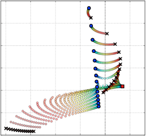
The stability map is shown in figure 5, where the abscissa displays the growth rate: the right half contains eigenfrequencies with positive growth rates, which yield unstable combustion. The computed eigenvalues correspond to cavity lengths  $0.05\ \textrm {m} \le L \le 0.18\ \textrm {m}$, for which a switch from unstable to stable combustion is reported (figure 1b). Note that the smallest cavity length tested experimentally is 0.085 m. For the sake of brevity, we concentrate on this first transition from unstable to stable combustion. The same mechanism accounts for the stability transitions at
 $0.35\ \textrm {m} \le L \le 0.45\ \textrm {m}$ and
 $0.70\ \textrm {m} \le L \le 0.75\ \textrm {m}$ (figure 1b).
Eigenvalues computed for the full, ITA and acoustic systems (figure 3). The coupling factor traces the path of both acoustic and ITA systems ( $\mu =0$) to the original full system (
 $\mu =1$). Cavity length is denoted as
 $L$, which varies from 0.05 m to 0.18 m. The acoustic and ITA modes are only computed for
 $\mu = 0$ at each cavity length. The acoustic mode for each cavity length corresponds to the first unstable mode.

The ITA system is unstable at 418 Hz (figure 5, red square), which is coherent with the  $-{\rm \pi}$ criterion for the phase of the FTF (figure 2) (Hoeijmakers et al. Reference Hoeijmakers, Kornilov, Arteaga, de Goey and Nijmeijer2014; Courtine et al. Reference Courtine, Selle and Poinsot2015; Emmert et al. Reference Emmert, Bomberg and Polifke2015). For
 $L\le 0.11\ \textrm {m}$, the ITA mode couples to very strongly damped full system modes at approximately 210 Hz. In contrast, the acoustic modes couple to the unstable full system modes, for which the highest growth rates are found for frequencies around
 $510\ \textrm {Hz}\pm 5\ \textrm {Hz}$ (figure 5), which is in agreement with experimental stability observations (figure 1b).
As the cavity length is further increased ( $L\ge 0.12\ \textrm {m}$), the nature of the unstable full system mode changes: now, the acoustic modes couple to the strongly damped full system modes at approximately 210 Hz, whereas the ITA mode couples to the unstable full system modes.
Figure 6 highlights the change in mode nature in more detail. Figure 6(a), for  $L=0.11\ \textrm {m}$, shows that the acoustic modes couple to the unstable full system mode, while the ITA mode couples to damped modes at approximately
 $210\ \textrm {Hz}$ for
 $\mu =1$. Figure 6(b) displays the stability map for
 $L=0.12\ \textrm {m}$. Conversely to figure 6(a), the damped full system mode originates from the acoustic mode and the ITA mode drives the unstable combustion process at frequencies of approximately 470 Hz. This change in mode nature is due to a branch switch. This pattern continues for the next cavity length
 $L=0.13\ \textrm {m}$ (figure 6c) but growth rates start to decay. Further increase of the cavity length
 $L > 0.13\ \textrm {m}$ drastically decreases the growth rates until the unstable mode becomes stable (figure 5). The location of the EP is roughly estimated as the intersection of the average mode distances in the area where no modes are active.
Branch switch and strong mode veering observed during change of cavity length  $L$, featuring typical characteristics of an EP. The branch switch appears for
 $L=0.12\ \textrm {m}$ in panel (b). Panels (a) and (c) display the nature of unstable modes before and after the branch switch, respectively. Arrows indicate increasing coupling factor. The expected EP location is marked with a cross.

To confirm the location of the EP, we use a contour integral method (Gavin, Miedlar & Polizzi Reference Gavin, Miedlar and Polizzi2018) as done by Mensah et al. (Reference Mensah, Magri, Silva, Buschmann and Moeck2018). Next, we applied the method to the present target configuration (figure 7). By varying the cavity length  $L$ and the coupling parameter
 $\mu$ in a small range, we found the exact location of the EP to be close to the estimated location (figure 6). Figure 7 features another property of EPs: when varying the cavity length for the constant coupling parameter
 $\mu =0.34$, the eigenvalue trajectories collide from opposite directions at the EP and, for further increase of
 $L$, veer off in a perpendicular direction. As discussed in Seyranian, Kirillov & Mailybaev (Reference Seyranian, Kirillov and Mailybaev2005) and Mensah et al. (Reference Mensah, Magri, Silva, Buschmann and Moeck2018), this veering pattern is a unique feature of EPs. Finally, we show that the inner product of the eigenfunction close to the EP is approximately unity (figure 8): this demonstrates that, at the EP, the eigenvalues and the corresponding eigenfunctions coalesce.
Computation of the exact EP location based on a contour integral method (Gavin et al. Reference Gavin, Miedlar and Polizzi2018). The cavity length  $L$ is varied from 0.115 m to 0.119 m (displayed by marker size) and the coupling factor
 $\mu$ from 0.30 to 0.38 (displayed by marker colour). The EP is located at
 $L=0.168\ \textrm {m}$ and
 $\mu =0.342$ (displayed by the cross marker).

Inner product computation of the eigenvectors. Values close to unity indicate that the eigenvectors are parallel. The EP is located at  $L=0.168\ \textrm {m}$ and
 $\mu =0.342$ (white panels).

In this work, the most striking consequences of an EP are found: (i) a region indicating large parameter sensitivities, (ii) where strong veering of mode paths is found (figure 5), and (iii) a branch switch that changes the nature of the instability (figure 6). We confirmed our results by computing the exact EP location and the corresponding (almost perfectly) parallel eigenvectors for the same frequency. The branch-switching behaviour provides a possible explanation for the experimentally observed sudden change in noise levels between 80 dB and 120 dB (figure 1b). We also highlight the fact that the ITA mode plays a significant role in the stability of this set-up. To the best of our knowledge, this point has not been reported before.
5. Conclusion
Only recently, the theoretical studies of Mensah et al. (Reference Mensah, Magri, Silva, Buschmann and Moeck2018) featured EPs located in the stable complex plane of prototypical, canonical test cases. In this study, we identify an unstable EP in the numerical stability map of an experimental combustion system. By tracing the nature of the full system modes, the mode paths displayed strong veering and a branch switch close to the EP. The latter was found in the unstable complex plane and triggered stability transition. The results reveal that the ITA feedback loop plays an important role in this stability transition.
The identification of EPs requires two parameters to be changed. In this study, we propose a numerical tool to study EPs that uses one physical parameter (the cavity length  $L$) together with a ‘virtual parameter’ (the coupling parameter
 $\mu$, which decouples the full system into acoustic and ITA modes to understand the nature of the thermoacoustic mode): it can also be used to reduce the experimental complexity of the set-up, as only one variation is needed instead of two.
Future work will focus on the impact of nonlinear forcing amplitudes to incorporate the experimentally reported Flame Describing Function.
Acknowledgements
We thank the anonymous reviewers whose comments helped to improve this paper.
Declaration of interests
The authors report no conflict of interest.
Appendix. Acoustic network model
Fluctuations of velocity  $u'$ and pressure
 $p'$ are linked via characteristic wave amplitudes:
 \begin{equation} f=\frac{1}{2} \left( \frac{p'}{\rho c} + u' \right ), \quad g=\frac{1}{2} \left( \frac{p'}{\rho c} - u' \right ). \end{equation}
From (A1), primitive variables can be computed via  $u'=f-g$ and
 $p'/\rho c = f+g$. The ratio of the characteristic waves describes reflection coefficients as
 $R_u=g_u/f_u$ and
 $R_d=f_d/g_d$. Using the definition of the acoustic impedance, these can be written as
 \begin{equation} \left. \begin{gathered} R_u = (Z_u+1)/(Z_u-1),\\ R_d = (Z_d-1)/(Z_d+1). \end{gathered} \right\} \end{equation}
The configuration shown in figure 3 contains acoustic elements up- and downstream of the flame, which can be lumped together as impedances  $Z_u$ and
 $Z_d$, respectively. Considering the flame as a compact element, the Rankine–Hugoniot jump conditions (Chu Reference Chu1953) formulate an acoustic flame model. Combining the compact flame element together with the upstream cross-sectional area change (figure 3), the scattering matrix is
 \begin{equation} \begin{bmatrix} f_u\\ g_d \end{bmatrix} = \begin{bmatrix} \dfrac{\alpha- \xi}{\alpha +\xi} & \dfrac{2}{\alpha+ \xi} & \dfrac{\theta}{\alpha+\xi} \\[10pt] \dfrac{2 \alpha \xi}{\alpha+ \xi} & \dfrac{\xi-\alpha}{\alpha+\xi} & \dfrac{\xi \theta}{\alpha+\xi} \end{bmatrix} \begin{bmatrix} f_d \\ g_u\\ \dot{q}' \end{bmatrix}, \end{equation}
where  $\dot {q}'=F(\omega )u'_u$ with
 $u'_u=f_u-g_u$. The system matrix
 $\boldsymbol {\mathcal {M}}$ is obtained by combining (A2) and (A3):
 \begin{equation} 0 = \underbrace{\begin{bmatrix} -1 & \dfrac{Z_u+1}{Z_u-1} & 0 & 0 & 0 & 0 \\[10pt] \dfrac{\alpha - \xi}{\alpha+ \xi} & -1 & 0 & \dfrac{2}{\alpha+\xi} & 0 & \dfrac{\theta}{\alpha+\xi} \\[10pt] \dfrac{2 \alpha \xi}{\alpha+ \xi} & 0 & -1 & \dfrac{\xi - \alpha}{\alpha+\xi} & 0 & \dfrac{\xi \theta}{\alpha+\xi} \\[10pt] 0 & 0 & \dfrac{Z_d - 1}{Z_d + 1} & -1 & 0 & 0 \\[10pt] 1 & -1 & 0 & 0 & -1 & 0 \\[10pt] 0 & 0 & 0 & 0 & F & -1 \end{bmatrix}}_{\boldsymbol{\mathcal{M}}} \begin{bmatrix} f_u\\ g_u\\ f_d \\ g_u \\ u'_u\\ \dot{q}' \end{bmatrix}, \end{equation}
Emmert et al. (Reference Emmert, Bomberg, Jaensch and Polifke2017) proposed to separate out the upstream outgoing wave  $g_u$ caused by the flame. From (A4), we find that (i) the heat release
 $\dot {q}'$ drives
 $g_u$ via
 ${\theta }/({\alpha +\xi })$, (ii)
 $g_u$ acts on
 $({Z_u+1})/({Z_u-1})$ via the upstream ingoing wave
 $f_u$ and (iii)
 $g_u$ also acts on the velocity fluctuation
 $u'_u$ by
 $-1$. The equations are rearranged such that
 $\dot {q}'$ directly affects
 $f_u$ and the coupling term
 $\mu$ is introduced:

By transforming the system, the dynamics are not modified, thus the characteristic equation and eigenvalues do not change, but now the system has a block matrix structure (3.4).



