1 Introduction
The study of axial dispersion of a solute with the effect of boundary absorption in a straight tube has always been an interesting topic of research due to its broad applications in the fields of environmental dynamics, chemical engineering, biomedical engineering and physiological fluid dynamics. Related to the theory of dispersion, some examples are the pollutant transport in the environment, chromatographic separations in chemical engineering, the mixing and the transportation of drugs or toxins in physiological systems.
At first, Taylor (Reference Taylor1953) introduced the method of solute dispersion in a steady laminar viscous fluid flow through a straight tube, analytically and experimentally. In this study, it was discussed that solute in the fluid is dispersed due to both radial molecular diffusion and the axial convection with the effective molecular diffusion coefficient,
 $D_{\mathit{eff}}$
, defined by
 $D_{\mathit{eff}}=R^{2}w_{m}^{2}/48D_{m}$
, where
 $D_{m}$
is molecular diffusivity,
 $w_{m}$
is the mean axial velocity and
 $R$
is the radius of the tube. A new approach to study on Taylor dispersion in steady flow was described by Aris (Reference Aris1956) using the method of moments. In this analysis, the asymptotic behaviour of second moment about the mean was analysed by incorporating the effect of axial molecular diffusion with the effective molecular diffusion coefficient,
 $D_{\mathit{eff}}$
, defined by
 $D_{\mathit{eff}}=D_{m}+R^{2}w_{m}^{2}/48D_{m}$
. The axial dispersion of solute in a pulsatile flow of viscous fluid through an infinitely long tube with the pulsating pressure gradient was investigated by Aris (Reference Aris1960) using the method of moments. These studies were analysed only on the dispersion of solute at large times after the injection in the fluid but did not give any information about the solute dispersion for small times after the injection. After that Gill & Sankarasubramanian (Reference Gill and Sankarasubramanian1970) proposed a generalized dispersion model for fully developed steady laminar flow in a tube which provides the idea of solute dispersion at each time after injection of solute in the fluid. Using this method of analysis, the study of solute dispersion with the effect of interphase mass transfer across the tube wall was analysed by Sankarasubramanian & Gill (Reference Sankarasubramanian and Gill1973) under the consideration of three effective transport coefficients i.e. exchange coefficient due to the irreversible first-order reaction at the tube wall, convective coefficient due to velocity of the solute and dispersion coefficient due to the molecular diffusion and the velocity of the fluid. This dispersion model is much more applicable in wide area of unsteady state heat and mass transfer problems.
Several researchers have applied the Taylor–Aris’s dispersion theory and the generalized dispersion model to analyse the dispersion process of solute in steady and oscillatory flows in the Newtonian fluid through a straight and curved tube or channel or annulus with and without the effect of absorption or irreversible first-order catalytic reaction at the boundary. The longitudinal dispersion of passive contaminant in oscillatory flows through a tube with an effective molecular diffusion coefficient,
 $D_{\mathit{eff}}$
was discussed by Chatwin (Reference Chatwin1975). Experimental results for axial transport of contaminant gas in oscillatory flow in a tube were obtained by Joshi et al. (Reference Joshi, Kamm, Drazen and Slutsky1983) to determine the effective molecular diffusion coefficient. Rao & Deshikachar (Reference Rao and Deshikachar1987) studied the axial dispersion of solute in a fully developed laminar steady flow through an annular pipe. The axial dispersion of a passive contaminant in a pulsatile flow of viscous incompressible fluid with the effect of first-order irreversible catalytic reaction at the tube wall was analysed by Mazumder & Das (Reference Mazumder and Das1992) following the method of moments. Using the Aris–Barton method of moments, Bandyopadhyay & Mazumder (Reference Bandyopadhyay and Mazumder1999) developed a dispersion model to study the effect of longitudinal dispersion process for the pulsatile flow in a channel. Based on the generalized dispersion model, the study of solute dispersion in a periodic flow through an annulus with the effect of irreversible boundary reaction was described by Sarkar & Jayaraman (Reference Sarkar and Jayaraman2004). By introducing the method of integral moments, Mazumder & Mondal (Reference Mazumder and Mondal2005) discussed on the dispersion process of passive tracer under the combined effects of frequency of pressure pulsation and first-order heterogeneous chemical reaction at the outer wall in a pulsatile flow through an annular pipe. The combined effects of heterogeneous reversible and irreversible wall reactions on dispersion of a chemical species in steady and oscillatory flows in a small diameter tube were studied by Ng (Reference Ng2006) using the multiple scale asymptotic analysis. The unsteady longitudinal dispersion of solute in oscillatory flow through a curved channel with absorbing walls using the Aris–Barton method of moments was analysed by Kumar & Jayaraman (Reference Kumar and Jayaraman2008). Imposing the method of integral moments, the analysis of longitudinal dispersion of solute in a periodic flow between two coaxial cylinders was presented by Paul (Reference Paul2011) to determine the longitudinal dispersion coefficient with the various of radius ratio, absorption parameter and frequency parameter.
The study of solute dispersion in an unsteady flow of non-Newtonian fluids has lots of applications in polymers, biochemical processing and cardiovascular flows. But little literature on dispersion processes can be found on non-Newtonian fluids. Following the theory of Taylor’s dispersion, the effective axial diffusion coefficient was determined by Sharp (Reference Sharp1993) in fully developed steady flow of non-Newtonian fluids such as Casson, power law and Bingham fluids in a straight tube. Based on Taylor’s dispersion model, the axial dispersion of solute in power law fluids through a circular curved tube was analysed by Agrawal & Jayaraman (Reference Agrawal and Jayaraman1994) for low Dean number,
 $Dn$
, defined by
 $Dn=Re/\sqrt{{\it\lambda}}$
, where
 $Re$
is the Reynolds number based on diameter of the tube and
 ${\it\lambda}$
is the curvature ratio. Hazra, Gupta & Niyogi (Reference Hazra, Gupta and Niyogi1997) presented a literature on solute dispersion in oscillatory flow of a viscoelastic non-Newtonian second-order fluid through a channel to obtain the longitudinal dispersion coefficient with the effects of viscoelastic parameter, amplitude and frequency of pressure pulsation by using the generalized dispersion model. Dash, Jayaraman & Mehta (Reference Dash, Jayaraman and Mehta2000) extended the study of Sharp (Reference Sharp1993) for unsteady solute dispersion in a Casson fluid in a pipe and channel under the presence of effective diffusion coefficient and the effect of yield stress of the fluid by using the approach of generalized dispersion model. The solute dispersion in a Casson fluid flow in a pipe and channel with the combined effect of yield stress and irreversible wall reaction was analysed by Nagarani, Sarojamma & Jayaraman (Reference Nagarani, Sarojamma and Jayaraman2004) using the generalized dispersion model. This study was extended by Nagarani, Sarojamma & Jayaraman (Reference Nagarani, Sarojamma and Jayaraman2009) in a Casson fluid flow in an annulus which has an application to catheterized artery under the presence of boundary reaction. But these studies of Nagarani et al. (Reference Nagarani, Sarojamma and Jayaraman2004, Reference Nagarani, Sarojamma and Jayaraman2009) were found to be applicable only for large time after the injection of the solute. Nagarani, Sarojamma & Jayaraman (Reference Nagarani, Sarojamma and Jayaraman2006) described the dispersion process of solute in the flow of a Casson fluid in an annulus by employing the generalized dispersion model with the effects of the yield stress and the annular gap. Applying the generalized dispersion model, the analysis of unsteady solute dispersion in the pulsatile flow of a Casson fluid in a tube was presented by Nagarani & Sebastian (Reference Nagarani and Sebastian2013) to determine the dispersion coefficient and the concentration of solute with the effects of Womersley frequency number, Schmidt number, yield stress and fluctuating pressure component. In this study, the effect of first-order reaction catalysed by the tube wall on the dispersion process has not been discussed.
In the present study, the unsteady axial dispersion of solute in the pulsatile flow of a non-Newtonian Casson fluid in a tube is analysed with the effect of an irreversible first-order boundary reaction. By following the generalized dispersion model proposed by Gill & Sankarasubramanian (Reference Gill and Sankarasubramanian1970) and Sankarasubramanian & Gill (Reference Sankarasubramanian and Gill1973), the solute transport in the fluid is analysed by considering three effective transport coefficients i.e. exchange, convection and dispersion coefficients. From this analysis, it is noticed that the convection and dispersion coefficient not only depend on time but also depend on the wall absorption parameter, yield stress, amplitude of fluctuating pressure component and Womersley frequency parameter in the presence of boundary reaction. The axial mean concentration of solute is also discussed with the effect of the boundary reaction, time, yield stress, fluctuating pressure component and frequency parameter. This study on dispersion process has wide application of blood flows due to pulsatile nature of the flow of blood (Nagarani et al. Reference Nagarani, Sarojamma and Jayaraman2004).
2 Mathematical formulation
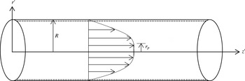
An unsteady, axisymmetric, fully developed, pulsatile flow of Casson fluid in a straight circular cylindrical tube of radius
 $R$
as shown in figure 1 is considered to analyse the axial dispersion of solute. In this study, one-dimensional flow is assumed. Due to an irreversible first-order catalytic reaction, solute is continuously absorbed by the tube wall and the rate of solute absorption is proportional to the solute concentration at the wall. In this study, free convection effects are neglected and a dilute solution is considered so that the product of reaction does not cause any coupling of flux (Sankarasubramanian & Gill Reference Sankarasubramanian and Gill1973).
2.1 Governing equation
The concentration of the solute is analysed by the unsteady convective diffusion equation
 $$\begin{eqnarray}\displaystyle \frac{\partial C^{\prime }}{\partial t^{\prime }}+w^{\prime }(t^{\prime },r^{\prime })\frac{\partial C^{\prime }}{\partial z^{\prime }}=D_{m}\left(\frac{1}{r^{\prime }}\frac{\partial }{\partial r^{\prime }}\left(r^{\prime }\frac{\partial C^{\prime }}{\partial r^{\prime }}\right)+\frac{\partial ^{2}C^{\prime }}{\partial z^{\prime 2}}\right), & & \displaystyle\end{eqnarray}$$
where
 $C^{\prime }$
is the local concentration of the solute,
 $w^{\prime }$
is the axial velocity of the fluid in tube,
 $D_{m}$
is the molecular diffusivity,
 $t^{\prime }$
is the time and
 $r^{\prime }$
and
 $z^{\prime }$
represent the radial and axial directions, respectively.
2.2 Initial and boundary conditions
(I) Initial condition:
Following Sankarasubramanian & Gill (Reference Sankarasubramanian and Gill1973), the initial solute distribution at
 $t^{\prime }=0$
is considered by introducing the solute of mass
 $M$
at the plane
 $z^{\prime }=0$
in a circular tube over the circular cross-section of radius
 $R$
. Hence, the initial concentration distribution may be written as
 $$\begin{eqnarray}\displaystyle C^{\prime }(0,z^{\prime },r^{\prime })=C_{0}{\it\psi}_{1}(z^{\prime })Y_{1}(r^{\prime }), & & \displaystyle\end{eqnarray}$$
with
 $$\begin{eqnarray}\displaystyle & \displaystyle C_{0}=\frac{M}{{\rm\pi}R^{3}}, & \displaystyle\end{eqnarray}$$
 $$\begin{eqnarray}\displaystyle & \displaystyle {\it\psi}_{1}(z^{\prime })=R{\it\delta}(z^{\prime }), & \displaystyle\end{eqnarray}$$
and
 $$\begin{eqnarray}\displaystyle & \displaystyle Y_{1}(r^{\prime })=1, & \displaystyle\end{eqnarray}$$
where
 ${\it\delta}(z^{\prime })$
is the Dirac delta function.
(II) Boundary conditions:
The following three boundary conditions are relevant for the present study.
-
(i) Condition due to symmetry
(2.6) $$\begin{eqnarray}\displaystyle \frac{\partial C^{\prime }}{\partial r^{\prime }}(t^{\prime },z^{\prime },0)=0. & & \displaystyle\end{eqnarray}$$
-
(ii) Condition due to the irreversible first-order heterogeneous reaction at the tube wall
(2.7)where
$$\begin{eqnarray}\displaystyle -D_{m}\frac{\partial C^{\prime }}{\partial r^{\prime }}(t^{\prime },z^{\prime },R)=kC^{\prime }(t^{\prime },z^{\prime },R), & & \displaystyle\end{eqnarray}$$
$k$
is the reaction rate constant.
-
(iii) Since the amount of solute in the system is finite, we shall have
(2.8)
$$\begin{eqnarray}\displaystyle C^{\prime }(t^{\prime },\infty ,r^{\prime })=\frac{\partial C^{\prime }}{\partial z^{\prime }}(t^{\prime },\infty ,r^{\prime })=0. & & \displaystyle\end{eqnarray}$$


2.3 Constitutive equation for Casson fluid and momentum equation
Following Aroesty & Gross (Reference Aroesty and Gross1972), the constitutive equation for Casson fluid in one dimensional shear flow may be written as
 $$\begin{eqnarray}\displaystyle & \displaystyle {\it\tau}^{\prime 1/2}={\it\tau}_{y}^{\prime 1/2}+\left(-{\it\mu}\frac{\partial w^{\prime }}{\partial r^{\prime }}\right)^{1/2},\quad \text{if}~{\it\tau}^{\prime }\geqslant {\it\tau}_{y}^{\prime }, & \displaystyle\end{eqnarray}$$
 $$\begin{eqnarray}\displaystyle & \displaystyle \frac{\partial w^{\prime }}{\partial r^{\prime }}=0,\quad \text{if}~{\it\tau}^{\prime }\leqslant {\it\tau}_{y}^{\prime }, & \displaystyle\end{eqnarray}$$
 ${\it\tau}^{\prime }$
and
 $\partial w^{\prime }/\partial r^{\prime }$
are the shear stress and shear rate, respectively,
 ${\it\tau}_{y}^{\prime }$
is the yield stress, and
 ${\it\mu}$
is the viscosity of Casson fluid (viscosity at high shear rate).
In the plug flow region in which shear stress
 ${\it\tau}^{\prime }$
is less than yield stress
 ${\it\tau}_{y}^{\prime }$
, the velocity gradients become zero. When shear rates in the fluid become very high i.e. for
 ${\it\tau}^{\prime }>{\it\tau}_{y}^{\prime }$
, Newtonian behaviour induces in the fluid. This behaviour is related to the blood flow in small tubes (Aroesty & Gross Reference Aroesty and Gross1972). The yield stress of the human blood is typically
 $0.04~\text{dyn cm}^{-2}$
at a hematocrit of 40 % (Merrill Reference Merrill1969).
Due to the pulsatile flow, the pressure gradient at any
 $z^{\prime }$
is represented by
 $$\begin{eqnarray}\displaystyle -\frac{\partial p^{\prime }}{\partial z^{\prime }}(t^{\prime })=P_{0}+P_{1}\sin ({\it\omega}t^{\prime }), & & \displaystyle\end{eqnarray}$$
where
 $P_{0}$
and
 $P_{1}$
are the steady and fluctuating components of the pressure gradient acting along the axis of tube,
 ${\it\omega}$
is the frequency of the pressure pulsation.
The momentum equation for Casson fluid is represented as
 $$\begin{eqnarray}\displaystyle {\it\rho}\frac{\partial w^{\prime }}{\partial t^{\prime }}=-\frac{\partial p^{\prime }}{\partial z^{\prime }}-\frac{1}{r^{\prime }}\frac{\partial }{\partial r^{\prime }}(r^{\prime }{\it\tau}^{\prime }), & & \displaystyle\end{eqnarray}$$
with boundary conditions
 $$\begin{eqnarray}{\it\tau}^{\prime }~\text{is finite}\quad \text{at}~r^{\prime }=0\end{eqnarray}$$
and
 $$\begin{eqnarray}w^{\prime }=0\quad \text{at}~r^{\prime }=R.\end{eqnarray}$$
2.4 Non-dimesionalization and velocity distribution
By introducing the following non-dimensional variables
 $$\begin{eqnarray}\displaystyle \left.\begin{array}{@{}c@{}}\displaystyle C=\frac{C^{\prime }}{C_{0}},\quad w=\frac{w^{\prime }}{w_{0}},\quad r=\frac{r^{\prime }}{R},\quad z=\frac{D_{m}z^{\prime }}{R^{2}w_{0}},\\ \displaystyle t=\frac{D_{m}t^{\prime }}{R^{2}},\quad {\it\tau}=\frac{{\it\tau}^{\prime }}{{\it\mu}(w_{0}/R)},\quad {\it\tau}_{y}=\frac{{\it\tau}_{y}^{\prime }}{{\it\mu}(w_{0}/R)},\quad e=\frac{P_{1}}{P_{0}},\end{array}\right\} & & \displaystyle\end{eqnarray}$$
the governing equation (2.1) transforms to
 $$\begin{eqnarray}\displaystyle \frac{\partial C}{\partial t}+w(t,r)\frac{\partial C}{\partial z}=\frac{1}{r}\frac{\partial }{\partial r}\left(r\frac{\partial C}{\partial r}\right)+\frac{1}{Pe^{2}}\frac{\partial ^{2}C}{\partial z^{2}}, & & \displaystyle\end{eqnarray}$$
where
 $w_{0}=(R^{2}/4{\it\mu})P_{0}$
is the characteristic velocity, and
 $Pe=Rw_{0}/D_{m}$
is the Peclet number.
The initial condition (2.2) and boundary conditions (2.6)–(2.8) can be written in non-dimensional form as:
 $$\begin{eqnarray}\displaystyle C(0,z,r)={\it\psi}(z)Y(r), & & \displaystyle\end{eqnarray}$$
with
 $$\begin{eqnarray}\displaystyle {\it\psi}(z)={\it\delta}(z)/Pe, & & \displaystyle\end{eqnarray}$$
and
 $$\begin{eqnarray}\displaystyle & \displaystyle Y(r)=1, & \displaystyle\end{eqnarray}$$
 $$\begin{eqnarray}\displaystyle & \displaystyle \frac{\partial C}{\partial r}(t,z,0)=0, & \displaystyle\end{eqnarray}$$
 $$\begin{eqnarray}\displaystyle & \displaystyle \frac{\partial C}{\partial r}(t,z,1)=-{\it\beta}C(t,z,1), & \displaystyle\end{eqnarray}$$
 $$\begin{eqnarray}\displaystyle & \displaystyle C(t,\infty ,r)=\frac{\partial C}{\partial z}(t,\infty ,r)=0, & \displaystyle\end{eqnarray}$$
where
 ${\it\beta}=kR/D_{m}$
is the wall absorption parameter.
Using the non-dimensional variables, the constitutive equation (2.9) reduces to
 $$\begin{eqnarray}\displaystyle & \displaystyle {\it\tau}^{1/2}={\it\tau}_{y}^{1/2}+\left(-\frac{\partial w}{\partial r}\right)^{1/2},\quad \text{if}~{\it\tau}\geqslant {\it\tau}_{y}, & \displaystyle\end{eqnarray}$$
 $$\begin{eqnarray}\displaystyle & \displaystyle \frac{\partial w}{\partial r}=0,\quad \text{if}~{\it\tau}\leqslant {\it\tau}_{y}. & \displaystyle\end{eqnarray}$$
 $$\begin{eqnarray}\displaystyle {\it\varepsilon}\frac{\partial w}{\partial t}=2p(t)-\frac{1}{r}\frac{\partial }{\partial r}(r{\it\tau}), & & \displaystyle\end{eqnarray}$$
with boundary conditions
 $$\begin{eqnarray}\displaystyle & \displaystyle {\it\tau}~\text{is finite}\quad \text{at}~r=0 & \displaystyle\end{eqnarray}$$
and
 $$\begin{eqnarray}\displaystyle w=0\quad \text{at}~r=1, & & \displaystyle\end{eqnarray}$$
where
 ${\it\varepsilon}=1/Sc$
,
 $p(t)=-2(\partial p^{\prime }/\partial z^{\prime })/P_{0}$
,
 $Sc={\it\nu}/D_{m}$
is the Schmidt number and
 ${\it\nu}$
is the kinematic viscosity coefficient.
Since the Schmidt number is very large
 $(O(10^{3}))$
in arterial blood flows (Caro et al.
Reference Caro, Pedley, Schroter and Seed1978), the parameter
 ${\it\varepsilon}$
is very small. In this study,
 ${\it\varepsilon}$
is treated as a perturbation parameter to obtain the velocity distribution for small as well as large values of Womersley frequency parameter
 ${\it\alpha}$
. Because of large values of
 $Sc$
, it is more appropriate to use this non-dimensionalization instead of the one that was given in Nagarani & Sebastian (Reference Nagarani and Sebastian2013).
By solving the nonlinear coupled equations (2.22) and (2.23) with perturbation analysis for small parameter
 ${\it\varepsilon}$
, the velocity distribution (Aroesty & Gross Reference Aroesty and Gross1972) in the plug flow region
 $(0\leqslant r\leqslant r_{p})$
is obtained as
 $$\begin{eqnarray}\displaystyle w_{1} & = & \displaystyle \frac{p(t)}{2}\left[1-\frac{8}{3}r_{p}^{1/2}+2r_{p}-\frac{1}{3}r_{p}^{2}\right]\nonumber\\ \displaystyle & & \displaystyle -\,{\it\varepsilon}\frac{p^{\prime }(t)}{32}\left[3-\frac{1144}{147}r_{p}^{1/2}+\frac{320}{63}r_{p}+\frac{4}{3}r_{p}^{2}-\frac{16}{9}r_{p}^{5/2}+\frac{65}{441}r_{p}^{4}\right],\quad \text{if}~0\leqslant r\leqslant r_{p},\nonumber\\ \displaystyle & & \displaystyle\end{eqnarray}$$
and that in the outside of plug region
 $(r_{p}\leqslant r\leqslant 1)$
is obtained as
 $$\begin{eqnarray}\displaystyle w_{2} & = & \displaystyle \frac{p(t)}{2}\left[(1-r^{2})-\frac{8}{3}r_{p}^{1/2}(1-r^{3/2})+2r_{p}(1-r)\right]\nonumber\\ \displaystyle & & \displaystyle -\,{\it\varepsilon}\frac{p^{\prime }(t)}{2}\left[\frac{3}{16}-\frac{r^{2}}{16}(4-r^{2})-\frac{r_{p}^{1/2}}{16}\left(\frac{1144}{147}-\frac{16}{3}(r^{2}+r^{3/2})+\frac{424}{147}r^{7/2}\right)\right]\nonumber\\ \displaystyle & & \displaystyle -\,{\it\varepsilon}p^{\prime }(t)\frac{r_{p}}{32}\left[\frac{320}{63}+\frac{128}{63}r^{3}-\frac{64}{9}r^{3/2}\right],\quad \text{if}~r_{p}\leqslant r\leqslant 1.\end{eqnarray}$$
In the above equations for velocity,
 $p(t)=2(1+e\sin ({\it\alpha}^{2}Sc\,t))$
,
 ${\it\alpha}^{2}={\it\omega}R^{2}/({\it\mu}/{\it\rho})$
,
 ${\it\alpha}$
is known as Womersley frequency parameter,
 $e$
is the amplitude of the fluctuating pressure component,
 $r_{p}={\it\tau}_{y}/p(t)$
is the dimensionless radius of the plug flow region and
 $p^{\prime }(t)=\text{d}p/\text{d}t$
. The product
 ${\it\alpha}^{2}Sc$
is the ratio of characteristic time of diffusion to the period of oscillation.
3 Method of solution
The unsteady convective diffusion equation (2.15) along with the initial and boundary conditions (2.16)–(2.21) is solved using the method suggested in Sankarasubramanian & Gill (Reference Sankarasubramanian and Gill1973). The solute concentration
 $C(t,z,r)$
is expanded in an infinite series as
 $$\begin{eqnarray}\displaystyle C(t,z,r)=\mathop{\sum }_{i=0}^{\infty }f_{i}(t,r)\frac{\partial ^{i}C_{m}(t,z)}{\partial z^{i}}, & & \displaystyle\end{eqnarray}$$
where the dimensionless mean concentration
 $C_{m}(t,z)$
is defined by
 $$\begin{eqnarray}\displaystyle C_{m}(t,z)=2\int _{0}^{1}Cr\,\text{d}r, & & \displaystyle\end{eqnarray}$$
and
 $f_{i}$
(
 $i=0,1,2,\ldots$
) are functions of
 $t$
and
 $r$
.
After multiplying by
 $2r$
and integrating with respect to
 $r$
from 0 to 1, the non-dimensional form of the governing equation (2.15) can be rewritten as
 $$\begin{eqnarray}\displaystyle \frac{\partial C_{m}}{\partial t}=\frac{1}{Pe^{2}}\frac{\partial ^{2}C_{m}}{\partial z^{2}}+2\frac{\partial C}{\partial r}(t,z,1)-2\frac{\partial }{\partial z}\int _{0}^{1}w(t,r)C(t,z,r)r\,\text{d}r. & & \displaystyle\end{eqnarray}$$
By substituting (3.1) into (3.3), the following dispersion model for
 $C_{m}$
is derived:
 $$\begin{eqnarray}\displaystyle \frac{\partial C_{m}}{\partial t}=\mathop{\sum }_{i=0}^{\infty }K_{i}(t)\frac{\partial ^{i}C_{m}}{\partial z^{i}}, & & \displaystyle\end{eqnarray}$$
where
 $$\begin{eqnarray}\displaystyle K_{i}(t)=\frac{{\it\delta}_{i2}}{Pe^{2}}+2\frac{\partial f_{i}}{\partial r}(t,1)-2\int _{0}^{1}f_{i-1}(t,r)w(t,r)r\,\text{d}r,\quad i=0,1,2,\ldots , & & \displaystyle\end{eqnarray}$$
and
 ${\it\delta}_{ij}$
denotes Kronecker delta
 $$\begin{eqnarray}{\it\delta}_{ij}=\left\{\begin{array}{@{}ll@{}}1, & i=j,\\ 0, & i\neq j.\end{array}\right.\end{eqnarray}$$
In (3.4), the terms involving
 $K_{i}(t)$
(
 $i=\text{3, 4, 5, }\ldots \text{}$
) can be neglected as their contribution is not significant (Gill & Sankarasubramanian Reference Gill and Sankarasubramanian1970). Then the resulting generalized dispersion model for mean concentration
 $C_{m}(t,z)$
is represented as
 $$\begin{eqnarray}\displaystyle \frac{\partial C_{m}}{\partial t}=K_{0}(t)C_{m}+K_{1}(t)\frac{\partial C_{m}}{\partial z}+K_{2}(t)\frac{\partial ^{2}C_{m}}{\partial z^{2}}, & & \displaystyle\end{eqnarray}$$
where
 $$\begin{eqnarray}\displaystyle K_{i}(t)=\frac{{\it\delta}_{i2}}{Pe^{2}}+2\frac{\partial f_{i}}{\partial r}(t,1)-2\int _{0}^{1}f_{i-1}(t,r)w(t,r)r\,\text{d}r,\quad i=0,1,2. & & \displaystyle\end{eqnarray}$$
In this study,
 $K_{0}(t)$
,
 $K_{1}(t)$
, and
 $K_{2}(t)$
are the exchange coefficient due to non-zero solute flux at the tube wall, convection coefficient due to the velocity of solute and dispersion coefficient due to the molecular diffusion and the velocity of the fluid, respectively. Due to the presence of pulsatile flow, both the coefficients
 $K_{1}(t)$
and
 $K_{2}(t)$
are the periodic functions of time (Chatwin Reference Chatwin1975; Sarkar & Jayaraman Reference Sarkar and Jayaraman2004).
Now the solute concentration
 $C(t,z,r)$
can be expanded in a finite series as
 $$\begin{eqnarray}\displaystyle C(t,z,r)=\mathop{\sum }_{i=0}^{2}f_{i}(t,r)\frac{\partial ^{i}C_{m}(t,z)}{\partial z^{i}}. & & \displaystyle\end{eqnarray}$$
Substituting (3.7) and (3.9) into (2.15), and equating the coefficients of
 $\partial ^{n}C_{m}/\partial z^{n}$
(
 $n=0,1,2$
), the set of differential equations for
 $f_{n}$
are obtained as
 $$\begin{eqnarray}\displaystyle \frac{\partial f_{n}}{\partial t}=\frac{1}{r}\frac{\partial }{\partial r}\left(r\frac{\partial f_{n}}{\partial r}\right)-w(t,r)f_{n-1}+\frac{1}{Pe^{2}}f_{n-2}-\mathop{\sum }_{i=0}^{n}K_{i}(t)f_{n-i}, & & \displaystyle\end{eqnarray}$$
where
 $n=0$
, 1, 2, and
 $f_{-1}=f_{-2}=0$
.
Using (3.2) and (3.9) in the initial and boundary conditions (2.16)–(2.21), the coefficients
 $C_{m}$
and
 $f_{n}$
are expressed as
 $$\begin{eqnarray}\displaystyle & \displaystyle C_{m}(0,z)=2{\it\psi}(z)\int _{0}^{1}Y(r)r\,\text{d}r, & \displaystyle\end{eqnarray}$$
 $$\begin{eqnarray}\displaystyle & \displaystyle f_{0}(0,r)=\frac{Y(r)}{2\displaystyle \int _{0}^{1}Y(r)r\,\text{d}r}, & \displaystyle\end{eqnarray}$$
 $$\begin{eqnarray}\displaystyle & \displaystyle f_{n}(0,r)=0,\quad n=1,2, & \displaystyle\end{eqnarray}$$
 $$\begin{eqnarray}\displaystyle & \displaystyle \frac{\partial f_{n}}{\partial r}(t,0)=0,\quad n=0,1,2, & \displaystyle\end{eqnarray}$$
 $$\begin{eqnarray}\displaystyle & \displaystyle \frac{\partial f_{n}}{\partial r}(t,1)=-{\it\beta}f_{n}(t,1),\quad n=0,1,2, & \displaystyle\end{eqnarray}$$
and
 $$\begin{eqnarray}\displaystyle & \displaystyle C_{m}(t,\infty )=\frac{\partial C_{m}}{\partial z}(t,\infty )=0. & \displaystyle\end{eqnarray}$$
Now using the definition of mean concentration
 $C_{m}(t,z)$
defined by (3.2) into (3.9), we have
 $$\begin{eqnarray}\displaystyle \int _{0}^{1}f_{n}(t,r)r\,\text{d}r=\frac{1}{2}{\it\delta}_{n0},\quad n=0,1,2, & & \displaystyle\end{eqnarray}$$
where
 ${\it\delta}_{n0}$
denotes as Kronecker delta described in (3.6).
The unknown functions
 $f_{0}$
,
 $K_{0}$
,
 $f_{1}$
,
 $K_{1}$
,
 $f_{2}$
and
 $K_{2}$
are obtained by solving the coupled system of partial differential equations (3.8) and (3.10). The method of eigenfunction expansion is used to determine the effective transport coefficients
 $K_{i}$
,
 $i=0,1,2$
.
3.1 Estimation of
$f_{0}(t,r)$
and
$K_{0}(t)$


The equation involving
 $f_{0}(t,r)$
and exchange coefficient
 $K_{0}(t)$
can be written from (3.10) as
 $$\begin{eqnarray}\displaystyle \frac{\partial f_{0}}{\partial t}=\frac{1}{r}\frac{\partial }{\partial r}\left(r\frac{\partial f_{0}}{\partial r}\right)-f_{0}K_{0}, & & \displaystyle\end{eqnarray}$$
with the initial and boundary conditions (3.12), (3.14), (3.15) for
 $n=0$
, and an additional condition obtained from (3.17) as
 $$\begin{eqnarray}\displaystyle \int _{0}^{1}f_{0}(t,r)r\,\text{d}r=\frac{1}{2}. & & \displaystyle\end{eqnarray}$$
Using the method of eigenfunction expansion, the solution of non-homogeneous boundary value problem (3.18) for
 $f_{0}(t\text{,}\,\,r)$
satisfying the initial and boundary conditions (3.12), (3.14), (3.15) and the condition (3.19) is obtained as (Boyce, DiPrima & Haines Reference Boyce, DiPrima and Haines1992)
 $$\begin{eqnarray}\displaystyle f_{0}(t,r)=\frac{\displaystyle \mathop{\sum }_{n=0}^{\infty }A_{n}\text{J}_{0}({\it\mu}_{n}r)\text{e}^{-{\it\mu}_{n}^{2}t}}{2\displaystyle \mathop{\sum }_{n=0}^{\infty }(A_{n}/{\it\mu}_{n})\text{J}_{1}({\it\mu}_{n})\text{e}^{-{\it\mu}_{n}^{2}t}}, & & \displaystyle\end{eqnarray}$$
where
 $\text{J}_{0}$
and
 $\text{J}_{1}$
are the Bessel functions of the first kind of order zero and one, respectively and
 ${\it\mu}_{n}$
are the roots of transcendental equation
 $$\begin{eqnarray}\displaystyle {\it\mu}_{n}\text{J}_{1}({\it\mu}_{n})={\it\beta}\text{J}_{0}({\it\mu}_{n}),\quad n=0,1,2,\ldots & & \displaystyle\end{eqnarray}$$
and
 $$\begin{eqnarray}\displaystyle A_{n}=\frac{{\it\mu}_{n}^{2}\displaystyle \int _{0}^{1}rY(r)\text{J}_{0}({\it\mu}_{n}r)\,\text{d}r}{({\it\mu}_{n}^{2}+{\it\beta}^{2})\text{J}_{0}^{2}({\it\mu}_{n})\displaystyle \int _{0}^{1}rY(r)\,\text{d}r},\quad n=0,1,2,\ldots . & & \displaystyle\end{eqnarray}$$
From (3.8) and (3.20)–(3.22), we obtain the exchange coefficient
 $K_{0}(t)$
as
 $$\begin{eqnarray}\displaystyle K_{0}(t)=2\frac{\partial f_{0}}{\partial r}(t,1)=-\frac{\displaystyle \mathop{\sum }_{n=0}^{\infty }A_{n}{\it\mu}_{n}\text{J}_{1}({\it\mu}_{n})\text{e}^{-{\it\mu}_{n}^{2}t}}{\displaystyle \mathop{\sum }_{n=0}^{\infty }(A_{n}/{\it\mu}_{n})\text{J}_{1}({\it\mu}_{n})\text{e}^{-{\it\mu}_{n}^{2}t}}, & & \displaystyle\end{eqnarray}$$
which is exactly the same as derived by Sankarasubramanian & Gill (Reference Sankarasubramanian and Gill1973). It is seen that
 $K_{0}(t)$
is independent of velocity field.
3.2 Estimation of
$f_{1}(t,r)$
and
$K_{1}(t)$


The governing equation for
 $f_{1}(t,r)$
and the convection coefficient
 $K_{1}(t)$
is derived from (3.10) by taking
 $n=1$
and is written as
 $$\begin{eqnarray}\displaystyle \frac{\partial f_{1}}{\partial t}=\frac{1}{r}\frac{\partial }{\partial r}\left(r\frac{\partial f_{1}}{\partial r}\right)-f_{1}K_{0}-(w(t,r)+K_{1})f_{0}. & & \displaystyle\end{eqnarray}$$
The appropriate initial and boundary conditions are given in (3.13)–(3.15) and we have also an additional condition obtained from (3.17) as
 $$\begin{eqnarray}\displaystyle \int _{0}^{1}f_{1}(t,r)r\,\text{d}r=0. & & \displaystyle\end{eqnarray}$$
The eigenfunction expansion solution for
 $f_{1}(t,r)$
satisfying the initial and boundary conditions (3.13)–(3.15) and the condition (3.25) is obtained as
 $$\begin{eqnarray}\displaystyle f_{1}(t,r)=-\frac{\displaystyle \mathop{\sum }_{n=0}^{\infty }\left[\displaystyle \mathop{\sum }_{m=0}^{\infty }B_{1mn}\left(\displaystyle \int _{0}^{t}\text{e}^{-({\it\mu}_{m}^{2}-{\it\mu}_{n}^{2})s}D_{mn}(s)\,\text{d}s\right)+B_{2n}F_{1}(t)\right]\text{J}_{0}({\it\mu}_{n}r)\text{e}^{-{\it\mu}_{n}^{2}t}}{2\displaystyle \mathop{\sum }_{n=0}^{\infty }(A_{n}/{\it\mu}_{n})\text{J}_{1}({\it\mu}_{n})\text{e}^{-{\it\mu}_{n}^{2}t}},\qquad & & \displaystyle\end{eqnarray}$$
where
 $$\begin{eqnarray}\displaystyle F_{1}(t) & = & \displaystyle \int _{0}^{t}K_{1}(s)\,\text{d}s\nonumber\\ \displaystyle & = & \displaystyle -\frac{\displaystyle \mathop{\sum }_{n=0}^{\infty }\displaystyle \mathop{\sum }_{m=0}^{\infty }B_{1mn}\left({\displaystyle \frac{\text{J}_{1}({\it\mu}_{n})}{{\it\mu}_{n}}}\right)\left(\displaystyle \int _{0}^{t}\text{e}^{-({\it\mu}_{m}^{2}-{\it\mu}_{n}^{2})s}D_{mn}(s)\,\text{d}s\right)\text{e}^{-{\it\mu}_{n}^{2}t}}{\displaystyle \mathop{\sum }_{n=0}^{\infty }B_{2n}\left({\displaystyle \frac{\text{J}_{1}({\it\mu}_{n})}{{\it\mu}_{n}}}\right)\text{e}^{-{\it\mu}_{n}^{2}t}},\end{eqnarray}$$
 $$\begin{eqnarray}\displaystyle D_{mn}(s) & = & \displaystyle \int _{0}^{1}rw(s,r)\text{J}_{0}({\it\mu}_{m}r)\text{J}_{0}({\it\mu}_{n}r)\,\text{d}r\nonumber\\ \displaystyle & = & \displaystyle w_{1}(s)\int _{0}^{r_{p}}r\text{J}_{0}({\it\mu}_{m}r)\text{J}_{0}({\it\mu}_{n}r)\,\text{d}r+\int _{r_{p}}^{1}rw_{2}(s,r)\text{J}_{0}({\it\mu}_{m}r)\text{J}_{0}({\it\mu}_{n}r)\,\text{d}r,\qquad\end{eqnarray}$$
 $$\begin{eqnarray}\displaystyle \left.\begin{array}{@{}c@{}}\displaystyle B_{1mn}=A_{m}A_{n}^{\prime 2},\quad B_{2n}=A_{n}A_{n}^{\prime 2}\left(\frac{\text{J}_{0}^{2}({\it\mu}_{n})+\text{J}_{1}^{2}({\it\mu}_{n})}{2}\right),\\ \displaystyle A_{n}=\frac{\left({\it\mu}_{n}^{2}\displaystyle \int _{0}^{1}rY(r)\text{J}_{0}({\it\mu}_{n}r)\,\text{d}r\right)}{({\it\mu}_{n}^{2}+{\it\beta}^{2})\text{J}_{0}^{2}({\it\mu}_{n})\displaystyle \int _{0}^{1}rY(r)\,\text{d}r},\quad A_{n}^{\prime 2}=\frac{2{\it\mu}_{n}^{2}}{({\it\mu}_{n}^{2}+{\it\beta}^{2})\text{J}_{0}^{2}({\it\mu}_{n})},\end{array}\right\} & & \displaystyle\end{eqnarray}$$
 $m=0,1,2,\ldots$
,
 $n=0,1,2,\ldots$
, and
 ${\it\mu}_{n}$
are the roots of transcendental equation
 $$\begin{eqnarray}\displaystyle {\it\mu}_{n}\text{J}_{1}({\it\mu}_{n})={\it\beta}\text{J}_{0}({\it\mu}_{n}),\quad n=0,1,2,\ldots . & & \displaystyle\end{eqnarray}$$
From (3.8),
 $K_{1}(t)$
is obtained and it is represented as
 $$\begin{eqnarray}\displaystyle K_{1}(t)=2\frac{\partial f_{1}}{\partial r}(t,1)-2\int _{0}^{1}f_{0}(t,r)w(t,r)r\,\text{d}r, & & \displaystyle\end{eqnarray}$$
where
 $$\begin{eqnarray}\displaystyle \frac{\partial f_{1}}{\partial r}(t,1)=\frac{\displaystyle \mathop{\sum }_{n=0}^{\infty }\left[\displaystyle \mathop{\sum }_{m=0}^{\infty }B_{1mn}\left(\displaystyle \int _{0}^{t}\text{e}^{-({\it\mu}_{m}^{2}-{\it\mu}_{n}^{2})s}D_{mn}(s)\,\text{d}s\right)+B_{2n}F_{1}(t)\right]{\it\mu}_{n}\text{J}_{1}({\it\mu}_{n})\text{e}^{-{\it\mu}_{n}^{2}t}}{2\displaystyle \mathop{\sum }_{n=0}^{\infty }(A_{n}/{\it\mu}_{n})\text{J}_{1}({\it\mu}_{n})\text{e}^{-{\it\mu}_{n}^{2}t}}.\qquad & & \displaystyle\end{eqnarray}$$
Now from (3.31) using (3.20), (3.27)–(3.30) and (3.32), the convective coefficient
 $K_{1}(t)$
is obtained numerically using the Simpson’s
 $1/3$
rule for integration.
3.3 Estimation of
$f_{2}(t,r)$
and
$K_{2}(t)$


By taking
 $n=2$
in (3.10), we obtain the equation for
 $f_{2}(t,r)$
involving the dispersion coefficient
 $K_{2}(t)$
as
 $$\begin{eqnarray}\displaystyle \frac{\partial f_{2}}{\partial t}=\frac{1}{r}\frac{\partial }{\partial r}\left(r\frac{\partial f_{2}}{\partial r}\right)-f_{2}K_{0}+\left(\frac{1}{Pe^{2}}-K_{2}\right)f_{0}-(w(t,r)+K_{1})f_{1}. & & \displaystyle\end{eqnarray}$$
The initial and boundary conditions are obtained from (3.13)–(3.15) for
 $n=2$
, and the addition condition is given by
 $$\begin{eqnarray}\displaystyle \int _{0}^{1}f_{2}(t,r)r\,\text{d}r=0. & & \displaystyle\end{eqnarray}$$
Using the method of eigenfunction expansion, the solution of (3.33) for
 $f_{2}(t,r)$
satisfying the initial and boundary conditions (3.13)–(3.15) and the additional condition (3.34) is obtained as
 $$\begin{eqnarray}\displaystyle f_{2}(t,r)=\frac{\displaystyle \mathop{\sum }_{n=0}^{\infty }\left[\displaystyle \mathop{\sum }_{m=0}^{\infty }B_{3mn}\left(\displaystyle \mathop{\sum }_{k=0}^{\infty }F_{3mnk}(t)+F_{4mn}(t)\right)-B_{5n}F_{2}(t)+\displaystyle \mathop{\sum }_{m=0}^{\infty }B_{4n}F_{5mn}(t)\right]\text{J}_{0}({\it\mu}_{n}r)\text{e}^{-{\it\mu}_{n}^{2}t}}{2\displaystyle \mathop{\sum }_{n=0}^{\infty }(A_{n}/{\it\mu}_{n})\text{J}_{1}({\it\mu}_{n})\text{e}^{-{\it\mu}_{n}^{2}t}},\hspace{-12.0pt} & & \displaystyle \nonumber\\ \displaystyle & & \displaystyle\end{eqnarray}$$
where
 $$\begin{eqnarray}\displaystyle F_{2}(t) & = & \displaystyle \int _{0}^{t}\left(K_{2}(s)-\frac{1}{Pe^{2}}\right)\text{d}s\nonumber\\ \displaystyle & = & \displaystyle \frac{\displaystyle \mathop{\sum }_{n=0}^{\infty }\left[\displaystyle \mathop{\sum }_{m=0}^{\infty }B_{3mn}\left(\displaystyle \mathop{\sum }_{k=0}^{\infty }F_{3mnk}(t)+F_{4mn}(t)\right)+\displaystyle \mathop{\sum }_{m=0}^{\infty }B_{4n}F_{5mn}(t)\right]\left({\displaystyle \frac{\text{J}_{1}({\it\mu}_{n})}{{\it\mu}_{n}}}\right)\text{e}^{-{\it\mu}_{n}^{2}t}}{\displaystyle \mathop{\sum }_{n=0}^{\infty }B_{5n}{\displaystyle \frac{\text{J}_{1}({\it\mu}_{n})}{{\it\mu}_{n}}}\text{e}^{-{\it\mu}_{n}^{2}t}},\nonumber\\ \displaystyle & & \displaystyle\end{eqnarray}$$
 $$\begin{eqnarray}\displaystyle & \displaystyle F_{3mnk}(t)=A_{k}A_{m}^{\prime }\int _{0}^{t}\left[\text{e}^{-({\it\mu}_{m}^{2}-{\it\mu}_{n}^{2})s}\left(\int _{0}^{s}\text{e}^{-({\it\mu}_{k}^{2}-{\it\mu}_{m}^{2})s^{\prime }}D_{km}(s^{\prime })\,\text{d}s^{\prime }\right)D_{mn}(s)\right]\text{d}s, & \displaystyle\end{eqnarray}$$
 $$\begin{eqnarray}\displaystyle & \displaystyle F_{4mn}(t)=A_{m}A_{m}^{\prime }\left(\frac{\text{J}_{0}^{2}({\it\mu}_{m})+\text{J}_{1}^{2}({\it\mu}_{m})}{2}\right)\int _{0}^{t}\text{e}^{-({\it\mu}_{m}^{2}-{\it\mu}_{n}^{2})s}\left[\left(\int _{0}^{s}K_{1}(s^{\prime })\,\text{d}s^{\prime }\right)D_{mn}(s)\right]\text{d}s, & \displaystyle \nonumber\\ \displaystyle & & \displaystyle\end{eqnarray}$$
 $$\begin{eqnarray}\displaystyle & \displaystyle F_{5mn}(t)=\int _{0}^{t}\left[\int _{0}^{s}\left(E_{mn}(s^{\prime })+A_{n}A_{n}^{\prime }\left(\frac{\text{J}_{0}^{2}({\it\mu}_{n})+\text{J}_{1}^{2}({\it\mu}_{n})}{2}\right)K_{1}(s^{\prime })\right)\text{d}s^{\prime }\right]K_{1}(s)\,\text{d}s,\qquad & \displaystyle\end{eqnarray}$$
 $$\begin{eqnarray}\displaystyle & \displaystyle E_{mn}(s^{\prime })=A_{m}A_{n}^{\prime }\text{e}^{-({\it\mu}_{m}^{2}-{\it\mu}_{n}^{2})s^{\prime }}D_{mn}(s^{\prime }), & \displaystyle\end{eqnarray}$$
 $$\begin{eqnarray}\displaystyle D_{mn}(s) & = & \displaystyle \int _{0}^{1}rw(s,r)\text{J}_{0}({\it\mu}_{m}r)\text{J}_{0}({\it\mu}_{n}r)\,\text{d}r\nonumber\\ \displaystyle & = & \displaystyle w_{1}(s)\int _{0}^{r_{p}}r\text{J}_{0}({\it\mu}_{m}r)\text{J}_{0}({\it\mu}_{n}r)\,\text{d}r+\int _{r_{p}}^{1}rw_{2}(s,r)\text{J}_{0}({\it\mu}_{m}r)\text{J}_{0}({\it\mu}_{n}r)\,\text{d}r,\qquad\end{eqnarray}$$
 $$\begin{eqnarray}\displaystyle \left.\begin{array}{@{}c@{}}\displaystyle B_{3mn}=A_{m}^{\prime }A_{n}^{\prime \prime 2},\quad B_{4n}=A_{n}^{\prime }A_{n}^{\prime \prime 2}\left(\frac{\text{J}_{0}^{2}({\it\mu}_{n})+\text{J}_{1}^{2}({\it\mu}_{n})}{2}\right),\\ \displaystyle B_{5n}=A_{n}A_{n}^{\prime \prime 2}\left(\frac{\text{J}_{0}^{2}({\it\mu}_{n})+\text{J}_{1}^{2}({\it\mu}_{n})}{2}\right),\quad A_{n}=\frac{{\it\mu}_{n}^{2}\displaystyle \int _{0}^{1}rY(r)\text{J}_{0}({\it\mu}_{n}r)\,\text{d}r}{({\it\mu}_{n}^{2}+{\it\beta}^{2})\text{J}_{0}^{2}({\it\mu}_{n})\displaystyle \int _{0}^{1}rY(r)\,\text{d}r},\\ \displaystyle {A^{\prime }}_{n}=\frac{\sqrt{2}{\it\mu}_{n}}{\sqrt{({\it\mu}_{n}^{2}+{\it\beta}^{2})}\text{J}_{0}({\it\mu}_{n})},\quad A_{n}^{\prime \prime 2}=\frac{2{\it\mu}_{n}^{2}}{({\it\mu}_{n}^{2}+{\it\beta}^{2})\text{J}_{0}^{2}({\it\mu}_{n})},\end{array}\right\}\quad & & \displaystyle\end{eqnarray}$$
 $m=0,1,2,\ldots$
,
 $n=0,1,2,\ldots$
, and
 ${\it\mu}_{n}$
are the roots of transcendental equation
 $$\begin{eqnarray}\displaystyle {\it\mu}_{n}\text{J}_{1}({\it\mu}_{n})={\it\beta}\text{J}_{0}({\it\mu}_{n}),\quad n=0,1,2,\ldots . & & \displaystyle\end{eqnarray}$$
From (3.8),
 $K_{2}(t)$
is obtained as
 $$\begin{eqnarray}\displaystyle K_{2}(t)=\frac{1}{Pe^{2}}+2\frac{\partial f_{2}}{\partial r}(t,1)-2\int _{0}^{1}f_{1}(t,r)w(t,r)r\,\text{d}r, & & \displaystyle\end{eqnarray}$$
where
 $$\begin{eqnarray}\displaystyle \frac{\partial f_{2}}{\partial r}(t,1)=-\frac{\displaystyle \mathop{\sum }_{n=0}^{\infty }\left[\displaystyle \mathop{\sum }_{m=0}^{\infty }B_{3mn}\left(\displaystyle \mathop{\sum }_{k=0}^{\infty }F_{3mnk}(t)+F_{4mn}(t)\right)-B_{5n}F_{2}(t)+\displaystyle \mathop{\sum }_{m=0}^{\infty }B_{4n}F_{5mn}(t)\right]F_{6n}(t)}{2\displaystyle \mathop{\sum }_{n=0}^{\infty }(A_{n}/{\it\mu}_{n})\text{J}_{1}({\it\mu}_{n})\text{e}^{-{\it\mu}_{n}^{2}t}}\hspace{-9.60004pt} & & \displaystyle \nonumber\\ \displaystyle & & \displaystyle\end{eqnarray}$$
and
 $$\begin{eqnarray}\displaystyle F_{6n}(t)={\it\mu}_{n}\text{J}_{1}({\it\mu}_{n})\text{e}^{-{\it\mu}_{n}^{2}t}. & & \displaystyle\end{eqnarray}$$
Now from (3.44) using (3.26), (3.36)–(3.43), (3.45) and (3.46), the dispersion coefficient
 $K_{2}(t)$
is obtained numerically using the Simpson’s
 $1/3$
rule of integration.
3.4 Solution for mean concentration
$C_{m}(t,z)$

The solution of (3.7) satisfying the initial and boundary conditions (3.11), (3.16) is given by
 $$\begin{eqnarray}\displaystyle C_{m}(t,z)=\frac{1}{2Pe\sqrt{{\rm\pi}T}}\exp \left({\it\xi}-\frac{z_{1}^{2}}{4T}\right), & & \displaystyle\end{eqnarray}$$
where
 $$\begin{eqnarray}\displaystyle & \displaystyle {\it\xi}(t)=\int _{0}^{t}K_{0}({\it\eta})\,\text{d}{\it\eta}, & \displaystyle\end{eqnarray}$$
 $$\begin{eqnarray}\displaystyle & \displaystyle z_{1}(t,z)=z+\int _{0}^{t}K_{1}({\it\eta})\,\text{d}{\it\eta}, & \displaystyle\end{eqnarray}$$
and
 $$\begin{eqnarray}\displaystyle & \displaystyle T(t)=\int _{0}^{t}K_{2}({\it\eta})\,\text{d}{\it\eta}. & \displaystyle\end{eqnarray}$$
4 Results and discussion
This study is undertaken to analyse the dispersion process of a solute in the pulsatile flow of Casson fluid through a tube with the irreversible boundary reaction. The generalized dispersion model suggested by Sankarasubramanian & Gill (Reference Sankarasubramanian and Gill1973) is applied to determine the three effective transport coefficients, i.e. the exchange, convection and dispersion coefficients which describe the whole dispersion process of solute. In the present analysis, the effect of wall absorption parameter
 ${\it\beta}$
on these three coefficients, the effect of yield stress
 ${\it\tau}_{y}$
, the fluctuating pressure component
 $e$
and Womersley frequency parameter
 ${\it\alpha}$
on the convection and dispersion coefficients is analysed by fixing the Schmidt number
 $Sc=1000$
and Peclet number
 $Pe=1000$
. The Schmidt number
 $Sc$
which is the ratio of viscous diffusion to molecular diffusion, is taken as
 $O(10^{3})$
(Caro et al.
Reference Caro, Pedley, Schroter and Seed1978; Mazumder & Das Reference Mazumder and Das1992; Truskey, Yuan & Katz Reference Truskey, Yuan and Katz2004) in arterial blood flows. In accordance with the physical process considered in the present investigations, the value of Peclet number
 $Pe$
is considered as 1000 (Mazumder & Das Reference Mazumder and Das1992; Nagarani & Sebastian Reference Nagarani and Sebastian2013). The variations in axial mean concentration
 $C_{m}$
has been discussed with the effect of wall absorption, yield stress and flow pulsatility using the expressions given in (3.47) and (3.48a–c
).
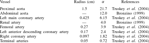
Values of Womersley frequency parameter
 ${\it\alpha}$
in human circulatory system.

In this study, the value of
 ${\it\beta}$
is taken in the range 0–100 to account for small and large absorption rates at the wall (Sankarasubramanian & Gill Reference Sankarasubramanian and Gill1973; Nagarani et al.
Reference Nagarani, Sarojamma and Jayaraman2004). The experimental values of
 ${\it\beta}$
are 0.7 for carbon dioxide, and
 ${\it\beta}\rightarrow \infty$
for acetaldehyde (Kaye, Kavafyan & Schroter Reference Kaye, Kavafyan and Schroter1993). By considering a small perturbation parameter
 ${\it\varepsilon}$
(
 $=\,1/Sc$
), the nonlinear coupled equations (2.22) and (2.23) are solved to analyse the velocity distribution of Casson fluid for both small and large values of the frequency parameter
 ${\it\alpha}$
. The parameter
 ${\it\alpha}$
is the ratio of unsteady inertial force to viscous force, and it can be rewritten as
 $R/\sqrt{({\it\nu}/{\it\omega})}$
or
 $\sqrt{2{\rm\pi}}R/\sqrt{({\it\nu}T)}$
, where
 $T$
is the period of pulsation. In the human circulatory system,
 ${\it\alpha}$
ranges from
 $O(10^{-3})$
in the capillaries to nearly 20 in the ascending aorta at rest (Caro et al.
Reference Caro, Pedley, Schroter and Seed1978; Chandran, Rittgers & Yoganathan Reference Chandran, Rittgers and Yoganathan2012). The values of
 ${\it\alpha}$
in human arteries are given in table 1. In this analysis,
 ${\it\alpha}$
is taken as 0.05, 0.1, 0.2, 0.5, 1, 2, 3, 3.05, 4, 6 and 10 to compare the present results with those existing in the literature. Due to pulsatile nature of the pressure, the velocity of the fluid is periodic in time with period
 $2{\rm\pi}/{\it\alpha}^{2}Sc$
and hence for
 ${\it\alpha}=0.05$
, 0.1, 0.2, 0.5, 1, 2, 3, 3.05, 4, 6 and 10, the time periods are calculated as 2.513, 0.628, 0.157, 0.025, 0.00628, 0.00157, 0.000698, 0.000675, 0.00039, 0.0001745 and 0.0000628, respectively. All the results in the present investigations are shown for three cycles of oscillation. Since the fluctuating pressure component
 $e$
varies from 0 to 1, its value is taken as 0.5 (Nagarani & Sebastian Reference Nagarani and Sebastian2013) in this study. The value of yield stress
 ${\it\tau}_{y}$
in the range 0–0.1 is appropriate for physiological flow situations in blood vessels (Dash, Jayaraman & Mehta Reference Dash, Jayaraman and Mehta1996). The value of
 ${\it\tau}_{y}$
is taken in the range 0–0.05 (Nagarani & Sebastian Reference Nagarani and Sebastian2013). The value of the diffusion coefficient in blood varies in the range
 $0.75\times 10^{-5}$
to
 $0.5\times 10^{-5}~\text{cm}^{2}~\text{s}^{-1}$
at a hematocrit of 33–45 % (Nagarani et al.
Reference Nagarani, Sarojamma and Jayaraman2004). When
 $e\rightarrow 0$
,
 ${\it\tau}_{y}=0$
and time is very large, the present results are found to be in agreement with Sankarasubramanian & Gill (Reference Sankarasubramanian and Gill1973) and Nagarani et al. (Reference Nagarani, Sarojamma and Jayaraman2004).
Integrals involved in the solution of convection coefficient
 $K_{1}(t)$
, dispersion coefficient
 $K_{2}(t)$
and mean concentration
 $C_{m}(t,z)$
are evaluated numerically using Simpson’s
 $1/3$
rule. It is seen that the exchange coefficient
 $K_{0}(t)$
depends on wall absorption parameter
 ${\it\beta}$
. The convection coefficient
 $K_{1}(t)$
and dispersion coefficient
 $K_{2}(t)$
depend on wall absorption parameter
 ${\it\beta}$
, yield stress
 ${\it\tau}_{y}$
, fluctuating pressure component
 $e$
of the fluid and Womersley frequency parameter
 ${\it\alpha}$
.
Schematic diagram of proposed model.

4.1 Exchange coefficient
$K_{0}(t)$

The amount of solute is continuously reduced in the tube due to the irreversible first-order reaction occurring at the tube wall. From (3.15) for
 $n=0$
and (3.23), it is seen that the exchange coefficient
 $K_{0}(t)$
directly depends on the wall absorption parameter
 ${\it\beta}$
. The coefficient
 $K_{0}(t)$
accounting for the non-zero solute flux at the tube wall will be negative for the depletion of solute in the system. At the time
 $t=0$
,
 $K_{0}$
becomes zero due to the absence of solute at the tube wall. As the time increases, solute moves along the tube and diffuses to the wall region. Due to which, the concentration of solute increases at the wall region. An equilibrium between the diffusive transport from the centre of the tube to the wall region and the reaction at the wall occurs due to which there is a steady state of the process and from that instant,
 $K_{0}$
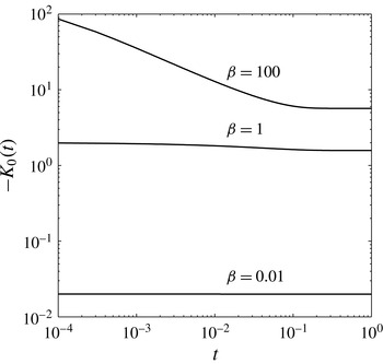
becomes constant. Figure 2 shows the variation of negative exchange coefficient
 $-K_{0}$
with time for
 ${\it\beta}=0.01$
, 1 and 100, respectively. From this figure, it is seen that there is no significant change in
 $-K_{0}$
with time
 $t$
for
 ${\it\beta}=0.01$
and
 ${\it\beta}=1$
. But the magnitude of
 $-K_{0}$
decreases rapidly as
 $t$
increases for large values of
 ${\it\beta}$
(
 ${\it\beta}=100$
is shown in the figure 2) and after a certain time it reaches a constant value. For small values of
 ${\it\beta}$
, an equilibrium between the diffusion of solute and the wall reaction occurs within small time and
 $K_{0}$
reaches the constant value. But, for large
 ${\it\beta}$
, as the time increases, solute in the system is reduced more rapidly due to the reaction at the wall and large time is taken to reach a steady state. From figure 2, it is also seen that as
 ${\it\beta}$
increases,
 $-K_{0}$
increases at initial time. The same phenomenon for
 $-K_{0}$
was reported for
 ${\it\beta}=0.01$
, 1 and 100 by Sankarasubramanian & Gill (Reference Sankarasubramanian and Gill1973).
Variation of negative exchange coefficient
 $-K_{0}(t)$
with time for wall absorption parameter
 ${\it\beta}=0.01$
, 1 and 100.

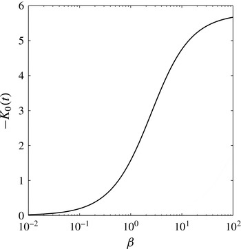
Figure 3 shows the variation of negative exchange coefficient
 $-K_{0}$
with
 ${\it\beta}$
at large time
 $t$
(Here the time
 $t=1$
is taken as very large). As
 ${\it\beta}$
increases, the magnitude of
 $-K_{0}$
increases continuously and becomes
 $5.669$
at
 $t=1$
for
 ${\it\beta}=100$
. Further, for very large values of
 ${\it\beta}$
, it approaches the value
 $5.78$
, as discussed in Sankarasubramanian & Gill (Reference Sankarasubramanian and Gill1973). The reason for this is because at sufficiently large value of
 ${\it\beta}$
, solute is consumed rapidly by the first-order reaction at the wall than it is supplied by the molecular diffusion and as a result the diffusion process is stabilized. It is worth mentioning that the exchange coefficient
 $K_{0}(t)$
is independent of the nature of the fluid (Newtonian/non-Newtonian) and the pulsatility of the vessels. Hence, the coefficient
 $K_{0}(t)$
is independent of
 ${\it\tau}_{y}$
,
 $e$
and
 ${\it\alpha}$
.
Variation of negative exchange coefficient
 $-K_{0}(t)$
at large time
 $t=1$
with wall absorption parameter
 ${\it\beta}$
.

4.2 Convection coefficient
$K_{1}(t)$

The convective coefficient
 $K_{1}$
is arising because of the fluid movement, unlike
 $K_{0}$
, the convection coefficient depends on yield stress of the fluid
 ${\it\tau}_{y}$
, amplitude of the fluctuating pressure component
 $e$
and frequency parameter
 ${\it\alpha}$
. In this analysis, the effects of
 ${\it\tau}_{y}$
,
 $e$
,
 ${\it\beta}$
and
 ${\it\alpha}$
on negative convection coefficient
 $-K_{1}$
have been discussed for small and large time.
The variation of negative convection coefficient
 $-K_{1}$
with small and large time for different values of yield stress
 ${\it\tau}_{y}$
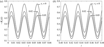
has been shown in figure 4(a,b). From these figures, it is seen that as
 ${\it\tau}_{y}$
increases, both the amplitude of fluctuations and the magnitude of
 $-K_{1}$
decreases. The coefficient
 $-K_{1}$
oscillates and reaches a non-transient state after certain period of time. For yield stress
 ${\it\tau}_{y}=0$
, 0.02 and 0.05,
 $-K_{1}$
starts to oscillate at initial time
 $t=0$
from the values 0.49, 0.384 and 0.329, respectively. So, solute is started initially to convect with the velocity of the fluid 0.49 along the tube for
 ${\it\tau}_{y}=0$
. At non-transient state in each period of oscillation,
 $-K_{1}$
reaches a constant value 0.74, 0.62 and 0.549 for
 ${\it\tau}_{y}=0$
, 0.02 and 0.05, respectively. Due to increase in
 ${\it\tau}_{y}$
or in other words, increase in the non-Newtonian parameter decreases the velocity of the fluid, which in turn caused a reduction in the value of
 $-K_{1}$
.
Variation of negative convection coefficient
 $-K_{1}(t)$
with
 $t$
for different values of
 ${\it\tau}_{y}$
when
 ${\it\beta}=0.01$
,
 ${\it\alpha}=0.5$
,
 $e=0.5$
and
 $Sc=1000$
. (a) For small times; (b) for large times.

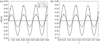
Figure 5(a,b) show the variation of
 $-K_{1}$
with small and large time for different values of fluctuating pressure component
 $e$
. It is observed from these figures that the amplitude of fluctuations of
 $-K_{1}$
increases with
 $e$
. The flow is steady for the case
 $e=0$
. In steady flow at non-transient state,
 $-K_{1}$
reaches a constant value 0.336, that means the solute is convected along the tube with the constant velocity of the fluid 0.336 for
 ${\it\tau}_{y}=0.05$
. For unsteady flow at non-transient state, the amplitude of fluctuations of
 $-K_{1}$
reaches a constant value 0.549 and 0.421 in each cycle of oscillation when
 $e=0.5$
and
 $e=0.2$
, respectively. The critical time for which
 $K_{1}$
reaches a non-transient state is independent of
 $e$
. As
 $e$
increases, fluctuating component of the pressure gradient increases and hence flow velocity increases which leads to increase in
 $-K_{1}$
.
Variation of negative convection coefficient
 $-K_{1}(t)$
with
 $t$
for different values of
 $e$
when
 ${\it\tau}_{y}=0.05$
,
 ${\it\beta}=0.01$
,
 ${\it\alpha}=0.5$
and
 $Sc=1000$
. (a) For small times; (b) for large times.

The variation of
 $-K_{1}$
has been shown at small and large time for different values of wall absorption parameter
 ${\it\beta}$
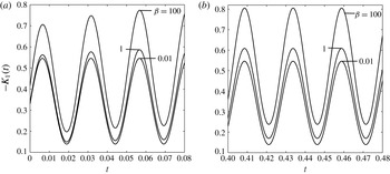
in figure 6. For
 ${\it\beta}=0.01$
, the fluctuation of
 $-K_{1}$
does not increase significantly and reaches a stationary state at small time after certain period of oscillation. But for
 ${\it\beta}=1$
and
 ${\it\beta}=100$
, the amplitude of oscillations of
 $-K_{1}$
increases at small time and becomes stable at large time. At each period of oscillation in stationary state,
 $-K_{1}$
reaches a constant value
 $0.809$
,
 $0.61$
and
 $0.549$
for
 ${\it\beta}=100$
, 1 and 0.01, respectively. It is evident from these figures that as
 ${\it\beta}$
increases, the amplitude of oscillations of
 $-K_{1}$
increases at small and large time. The growth of oscillations of
 $-K_{1}$
at small time becomes larger for larger values of
 ${\it\beta}$
. The reason for this enhancement of
 $-K_{1}$
at large value of
 ${\it\beta}$
is due to the consumption of solute in the presence of boundary absorption at the wall. Higher values of
 ${\it\beta}$
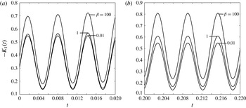
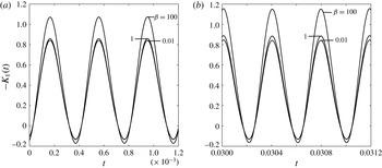
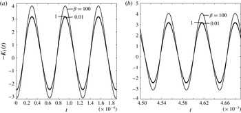
satisfies more absorption at the wall region and lesser solute is available for convection compared to that at the central region of the tube. So, the solute distribution is weighted in favour of the central region and solute is convected with faster velocity near the central region than that at the wall region. From the figures 7–9, it is also seen that as
 ${\it\beta}$
increases, the amplitude of oscillations of
 $-K_{1}$
increases for different values of
 ${\it\alpha}$
. But the difference between the amplitude of fluctuations of
 $-K_{1}$
for different values of
 ${\it\beta}$
decreases as
 ${\it\alpha}$
increases and becomes very small at large value of
 ${\it\alpha}$
.
Variation of negative convection coefficient
 $-K_{1}(t)$
with
 $t$
for different values of
 ${\it\beta}$
when
 ${\it\tau}_{y}=0.05$
,
 ${\it\alpha}=0.5$
,
 $e=0.5$
and
 $Sc=1000$
. (a) For small times; (b) for large times.

Variation of negative convection coefficient
 $-K_{1}(t)$
with
 $t$
for different values of
 ${\it\beta}$
when
 ${\it\tau}_{y}=0.05$
,
 ${\it\alpha}=1$
,
 $e=0.5$
and
 $Sc=1000$
. (a) For small times; (b) for large times.

Variation of negative convection coefficient
 $-K_{1}(t)$
with
 $t$
for different values of
 ${\it\beta}$
when
 ${\it\tau}_{y}=0.05$
,
 ${\it\alpha}=4$
,
 $e=0.5$
and
 $Sc=1000$
. (a) For small times; (b) for large times.

Variation of negative convection coefficient
 $-K_{1}(t)$
with
 $t$
for different values of
 ${\it\beta}$
when
 ${\it\tau}_{y}=0.05$
,
 ${\it\alpha}=10$
,
 $e=0.5$
and
 $Sc=1000$
. (a) For small times; (b) for large times.

The Womersley frequency parameter
 ${\it\alpha}$
is seen to have significant influence on
 $-K_{1}$
in the case of non-Newtonian fluid. Figures 6–9 show the variation of
 $-K_{1}$
with small and large time for different values of
 ${\it\alpha}=0.5$
,
 $1$
,
 $4$
and
 $10$
. It can be observed that the amplitude of fluctuation of
 $-K_{1}$
increases with
 ${\it\alpha}$
. The period of oscillation becomes short at large value of
 ${\it\alpha}$
. At small time, the fluctuation of
 $-K_{1}$
does not increase significantly for large values of
 ${\it\alpha}$
and
 $-K_{1}$
reaches a stationary state at small time. In each period of oscillation for
 ${\it\beta}=0.01$
,
 $-K_{1}$
reaches a constant value
 $0.549$
,
 $0.551$
,
 $0.845$
and
 $3.195$
at non-transient state for
 ${\it\alpha}=0.5$
,
 $1$
,
 $4$
and
 $10$
, respectively. It also seen that as
 ${\it\alpha}$
increases, the magnitude of
 $-K_{1}$
decreases initially at time
 $t=0$
but after that the amplitude of fluctuations of
 $-K_{1}$
increases more and becomes positive and negative during the period of oscillation. The negative value of
 $-K_{1}$
occurs due to the flow reversal in the period.
When
 $e=0$
and time
 $t$
is very large, the variation of negative convection coefficient
 $-K_{1}$
with
 ${\it\beta}$
for various values of the non-Newtonian parameter
 ${\it\tau}_{y}$
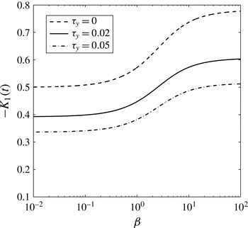
has been shown in figure 10. It is observed that as
 ${\it\beta}$
increases, the magnitude of
 $-K_{1}$
increases and it decreases as
 ${\it\tau}_{y}$
increases (Nagarani et al.
Reference Nagarani, Sarojamma and Jayaraman2004). The fluid velocity in Casson fluid is less compared to that of the Newtonian fluid and this leads to lesser convective coefficient in the Casson fluid. As
 ${\it\beta}\rightarrow \infty$
,
 $K_{1}\rightarrow -0.78$
for
 ${\it\tau}_{y}=0$
, i.e. as
 ${\it\beta}$
increases, the coefficient
 $-K_{1}$
increases and possesses to the value
 $0.78$
for
 ${\it\tau}_{y}=0$
. In the absence of wall absorption, i.e. for
 ${\it\beta}=0$
, the value of
 $-K_{1}$
is
 $0.5$
which means that solute is moved along the tube with the average velocity of the flow. As
 ${\it\beta}$
increases, solute is transported with the velocity higher than the average velocity of the flow. Similar profile for
 $-K_{1}$
with
 ${\it\tau}_{y}=0$
is seen in Sankarasubramanian & Gill (Reference Sankarasubramanian and Gill1973) and Nagarani et al. (Reference Nagarani, Sarojamma and Jayaraman2004).
Variation of negative convection coefficient
 $-K_{1}(t)$
for different values of
 ${\it\tau}_{y}$
with wall absorption parameter
 ${\it\beta}$
at large time
 $t=1$
when
 $e=0$
.

4.3 Dispersion coefficient
$K_{2}(t)$

The dispersion coefficient
 $K_{2}$
depends on the yield stress of the fluid
 ${\it\tau}_{y}$
, amplitude of the fluctuating pressure component
 $e$
, wall absorption parameter
 ${\it\beta}$
and frequency parameter
 ${\it\alpha}$
. In the present study, the effects of
 ${\it\tau}_{y}$
,
 $e$
,
 ${\it\beta}$
and
 ${\it\alpha}$
on solute dispersion have been discussed for small as well as large time.
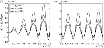
Figure 11(a,b) show the variation of dispersion coefficient
 $K_{2}$
(from which the additive contribution of the axial diffusion
 $1/Pe^{2}$
is deducted) with small and large time for different values of
 ${\it\tau}_{y}$
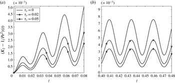
. From these figures, it is noticeable that as
 ${\it\tau}_{y}$
increases, both the amplitude of fluctuations and the magnitude of
 $K_{2}$
decreases. With the injection of solute in the blood flow, the solute dispersion starts within small time. At small time,
 $K_{2}$
increases periodically with wavy nature and thereafter decreases as time increases and reaches a non-transient state at large time
 $t$
, which is related to the characteristic time of transverse diffusion
 $R^{2}/D_{m}$
. After the initial increment of the amplitude of oscillation for small time as seen in figure 11(a), these oscillations become stable at large time as large as
 $t\geqslant 0.4$
(as shown in figure 11
b) and thereafter the dispersion of solute takes place with the period of oscillation at a uniform rate. Due to increase in
 ${\it\tau}_{y}$
, the velocity decreases and hence a decrease in the dispersion coefficient is noticed.
Variation of dispersion coefficient
 $(K_{2}-1/Pe^{2})(t)$
with
 $t$
for different values of
 ${\it\tau}_{y}$
when
 ${\it\beta}=0.01$
,
 ${\it\alpha}=0.5$
,
 $e=0.5$
and
 $Sc=1000$
. (a) For small times; (b) for large times.

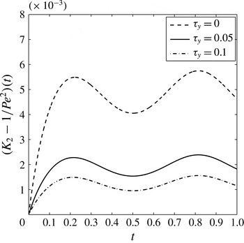
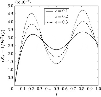
In figure 12(a,b), the variation of dispersion coefficient
 $K_{2}$
at all times is shown for steady flow
 $(e=0)$
of Newtonian fluid
 $({\it\tau}_{y}=0)$
and Casson fluid
 $({\it\tau}_{y}=0.05)$
with and without the effect of wall absorption (
 ${\it\beta}=0.01$
and
 ${\it\beta}=0$
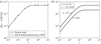
). Present result (shown in the figure 12
a) for steady flow of Newtonian fluid in the absence of wall absorption matches exactly with the result of Gill & Sankarasubramanian (Reference Gill and Sankarasubramanian1970) (figure 1) at small and large time. Also, our result for steady flow of Newtonian fluid with the effect of wall absorption is found to be in best agreement with Sankarasubramanian & Gill (Reference Sankarasubramanian and Gill1973) at very large time. From figure 12(a,b), it is seen that as time increases,
 $K_{2}$
increases rapidly at small time and reaches a constant value at large time
 $(t\geqslant 0.5)$
. For
 ${\it\tau}_{y}=0$
and
 ${\it\tau}_{y}=0.05$
with
 ${\it\beta}=0$
,
 $K_{2}$
reaches a constant value
 $5.21\times 10^{-3}$
and
 $2.13\times 10^{-3}$
, respectively at large time
 $(t\geqslant 0.5)$
. It is also observed that
 $K_{2}$
decreases as
 ${\it\tau}_{y}$
increases at small as well as large time. Also,
 $K_{2}$
decreases with the increment of wall absorption parameter
 ${\it\beta}$
. But the difference of
 $K_{2}$
between the case of
 ${\it\beta}=0$
and
 ${\it\beta}=0.01$
is small and for each case
 $K_{2}$
attains a same constant value at very large time
 $(t=10)$
.
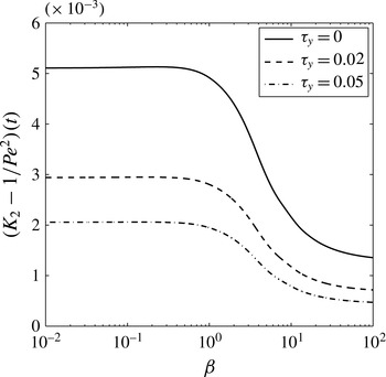
Variation of dispersion coefficient
 $(K_{2}-1/Pe^{2})(t)$
with
 $t$
for different values of
 ${\it\tau}_{y}$
and
 ${\it\beta}$
at small and large time when
 $e=0$
. The data of Gill & Sankarasubramanian (Reference Gill and Sankarasubramanian1970) for
 $K_{2}$
is obtained from the equations (19) and (20) of their paper. (a)
 ${\it\tau}_{y}=0$
with
 ${\it\beta}=0$
; (b)
 ${\it\tau}_{y}=0$
and 0.05 with
 ${\it\beta}=0$
and 0.01.

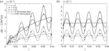
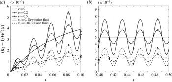
At small as well as large time, the variation of
 $K_{2}$
for different values of
 $e$
and
 ${\it\tau}_{y}$
has been presented for
 ${\it\beta}=0$
and
 ${\it\beta}=0.01$
in figures 13 and 14, respectively. For the clarity in comparison, these results are presented here for four cycles of oscillation for both Newtonian fluid
 $({\it\tau}_{y}=0)$
and Casson fluid
 $({\it\tau}_{y}=0.05)$
. From these figures, it is seen that as
 $e$
increases, both the amplitude of fluctuations and the magnitude of
 $K_{2}$
increases. For the steady flow,
 $K_{2}$
increases at small time and attains a value
 $4.04\times 10^{-3}$
at
 $t=0.1$
and
 $5.19\times 10^{-3}$
at
 $t=0.4$
for
 ${\it\beta}=0$
and
 ${\it\tau}_{y}=0$
. For
 ${\it\tau}_{y}=0$
with
 ${\it\beta}=0.01$
,
 $K_{2}$
reaches a value
 $3.89\times 10^{-3}$
at
 $t=0.1$
and
 $5.04\times 10^{-3}$
at
 $t=0.4$
. For the unsteady flow
 $(e>0)$
,
 $K_{2}$
increases cyclically at small time and reaches a stationary state at large time. At each cycle of oscillation in large time with
 ${\it\tau}_{y}=0$
and
 ${\it\beta}=0.01$
,
 $K_{2}$
reaches a constant value
 $6.1\times 10^{-3}$
and
 $7.64\times 10^{-3}$
for
 $e=0.2$
and
 $e=0.5$
, respectively. A similar nature is seen for other values of
 ${\it\tau}_{y}$
. The critical time at which
 $K_{2}$
reaches a non-transient state becomes independent of
 $e$
. It is worth noting that the value of
 $K_{2}$
at small time
 $t=0.1$
for steady flow of Newtonian fluid without wall absorption as observed by Nagarani & Sebastian (Reference Nagarani and Sebastian2013) (referred to their figure 5) is near about
 $1\times 10^{-3}$
which deviates much from the value
 $(4.04\times 10^{-3})$
of Gill & Sankarasubramanian (Reference Gill and Sankarasubramanian1970) (equations (19) and (20) therein, for
 $K_{2}$
).
Variation of dispersion coefficient
 $(K_{2}-1/Pe^{2})(t)$
with
 $t$
for different values of
 $e$
and
 ${\it\tau}_{y}$
when
 ${\it\beta}=0$
. (a) For small times; (b) for large times.

Variation of dispersion coefficient
 $(K_{2}-1/Pe^{2})(t)$
with
 $t$
for different values of
 $e$
and
 ${\it\tau}_{y}$
when
 ${\it\beta}=0.01$
. (a) For small times; (b) for large times.

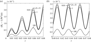
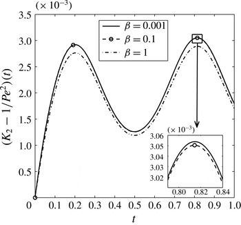
The effect on
 $K_{2}$
has been studied for different values of absorption parameter
 ${\it\beta}=0$
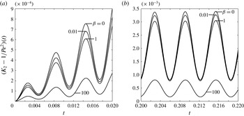
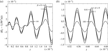
, 0.01, 1 and 100 with small and large time and it is shown in figures 15(a) and 15(b), respectively. It is observed from these figures that as
 ${\it\beta}$
increases, both the amplitude of fluctuations and the magnitude of
 $K_{2}$
decreases. Initially, the amplitude of oscillation of
 $K_{2}$
increases and reaches a constant value
 $3.56\times 10^{-3}$
,
 $3.42\times 10^{-3}$
,
 $3.2\times 10^{-3}$
and
 $0.81\times 10^{-3}$
at each period of oscillation in large time for
 ${\it\beta}=0$
, 0.01, 1 and 100, respectively. With increase in the value of
 ${\it\beta}$
, the dispersion coefficient
 $K_{2}$
decreases because number of moles of reactive material at the wall increases to undergo the chemical reaction or absorption and hence, more amount of solute near the wall is continuously depleted in the system. Therefore, the solute distribution is weighted in favour of the region near the centre of the tube and in this region, the solute is convected with the faster velocity than that near the wall region. So, the velocity gradients are smaller near the central region than near the wall and smaller gradients cause smaller dispersion. This could be a reason for decrease in axial dispersion when
 ${\it\beta}$
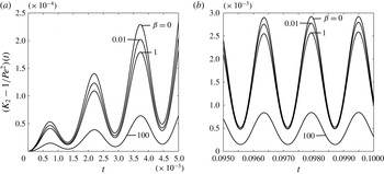
increases. Also, transverse diffusion of solute is increased by the larger transverse concentration gradients in the system with the presence of wall absorption and this causes the decrement in axial dispersion. From figures 16, 17 and 20–25, it is also noticed that the increase in
 ${\it\beta}$
tends to decrease the axial dispersion for various values of
 ${\it\alpha}$
.
Variation of dispersion coefficient
 $(K_{2}-1/Pe^{2})(t)$
with
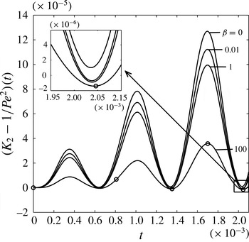
 $t$
for different values of
 ${\it\beta}$
when
 ${\it\tau}_{y}=0.05$
,
 ${\it\alpha}=0.5$
,
 $e=0.5$
and
 $Sc=1000$
. (a) For small times; (b) for large times.

Variation of dispersion coefficient
 $(K_{2}-1/Pe^{2})(t)$
with
 $t$
for different values of
 ${\it\beta}$
when
 ${\it\tau}_{y}=0.05$
,
 ${\it\alpha}=1$
,
 $e=0.5$
and
 $Sc=1000$
. (a) For small times; (b) for large times.

Variation of dispersion coefficient
 $(K_{2}-1/Pe^{2})(t)$
with
 $t$
for different values of
 ${\it\beta}$
when
 ${\it\tau}_{y}=0.05$
,
 ${\it\alpha}=2$
,
 $e=0.5$
and
 $Sc=1000$
. (a) For small times; (b) for large times.

Variation of dispersion coefficient
 $(K_{2}-1/Pe^{2})(t)$
with small time
 $t$
for different values of
 ${\it\tau}_{y}$
when
 ${\it\beta}=0.01$
,
 ${\it\alpha}=3$
,
 $e=0.5$
and
 $Sc=1000$
.

Variation of dispersion coefficient
 $(K_{2}-1/Pe^{2})(t)$
with small time
 $t$
for different values of
 ${\it\tau}_{y}$
when
 ${\it\beta}=0.01$
,
 ${\it\alpha}=3.05$
,
 $e=0.5$
and
 $Sc=1000$
.

Variation of dispersion coefficient
 $(K_{2}-1/Pe^{2})(t)$
with small time
 $t$
for different values of
 ${\it\beta}$
when
 ${\it\tau}_{y}=0.05$
,
 ${\it\alpha}=3$
,
 $e=0.5$
and
 $Sc=1000$
.

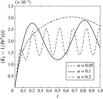
Variation of
 $K_{2}$
for small and large values of Womersley frequency parameter
 ${\it\alpha}$
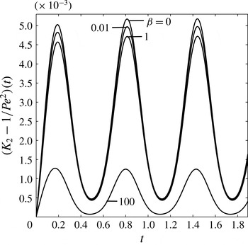
is shown through the figures 15–17 and 22–25 for small and large time. From these figures, it is seen that as
 ${\it\alpha}$
increases, the axial dispersion decreases. The amplitude of fluctuations of
 $K_{2}$
decreases at both small and large time as
 ${\it\alpha}$
increases. For all values of
 ${\it\alpha}$
,
 $K_{2}$
oscillates in increasing manner at small time and reaches a static state in oscillation at large time. In each period of oscillation for
 ${\it\beta}=0.01$
, the dispersion coefficient becomes stable at large time with a constant value
 $5\times 10^{-3}$
,
 $3.42\times 10^{-3}$
,
 $3.28\times 10^{-3}$
,
 $2.8\times 10^{-3}$
,
 $2.1\times 10^{-3}$
,
 $1.75\times 10^{-3}$
and
 $1.5\times 10^{-3}$
for
 ${\it\alpha}=0.1$
, 0.5, 1, 2, 4, 6 and 10, respectively. As
 ${\it\alpha}$
increases, amplitude of oscillations of
 $K_{2}$
decreases and
 $K_{2}$
becomes negative during the period of oscillation for large values of
 ${\it\alpha}$
. This nature also depends on
 ${\it\tau}_{y}$
,
 $e$
and
 ${\it\beta}$
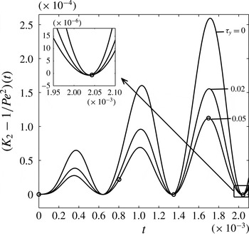
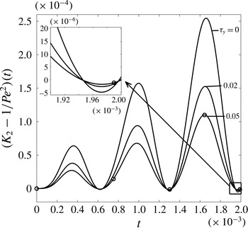
. From the figures 18 and 19, it is seen that
 $K_{2}$
attains the negative value within three cycles of oscillation in small time at
 ${\it\alpha}=3$
for different values of
 ${\it\tau}_{y}$
and as
 ${\it\tau}_{y}$
increases, the peak of negative dispersion increases for a value of
 ${\it\alpha}$
around
 ${\it\alpha}=3$
. With
 ${\it\alpha}=3.05$
, this phenomenon is shown in figure 19. Similar observations w.r.t.
 ${\it\beta}$
are shown in figures 20 and 21. From these figures, it is observed that for
 ${\it\beta}=0.01$
, 1 and 100,
 $K_{2}$
becomes negative at
 ${\it\alpha}=3$
but for
 ${\it\beta}=0$
,
 $K_{2}$
becomes negative at
 ${\it\alpha}=3.05$
within three cycles of oscillation in small time. So, negative dispersion is seen at
 ${\it\alpha}=3$
and the peak of negative dispersion increases with
 ${\it\alpha}$
. Womersley parameter directly depends on the radius of the vessel and its value is high in large vessels. The reversal of blood flow occurs in large vessels undergoing peristalsis (Craciunescu & Clegg Reference Craciunescu and Clegg2001). The backward flow is experienced during late systole and early diastole in the arteries such as carotid, brachial, femoral arteries, renal arteries and abdominal aorta in which the values of
 ${\it\alpha}$
are large (Ku Reference Ku1997). Due to the flow reversal in period, negative dispersion occurs and the material is moved back with the flow during the cycle of oscillation for large values of
 ${\it\alpha}$
(Mazumder & Das Reference Mazumder and Das1992). During the period of oscillation at each reversal of flow, the material dispersion is contracted (Smith Reference Smith1982).
Variation of dispersion coefficient
 $(K_{2}-1/Pe^{2})(t)$
with small time
 $t$
for different values of
 ${\it\beta}$
when
 ${\it\tau}_{y}=0.05$
,
 ${\it\alpha}=3.05$
,
 $e=0.5$
and
 $Sc=1000$
.

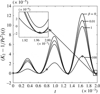
Variation of dispersion coefficient
 $(K_{2}-1/Pe^{2})(t)$
with
 $t$
for different values of
 ${\it\beta}$
when
 ${\it\tau}_{y}=0.05$
,
 ${\it\alpha}=4$
,
 $e=0.5$
and
 $Sc=1000$
. (a) For small times; (b) for large times.

From figures 15–17, it can be seen that fluctuation of
 $K_{2}$
increases cyclically in small time with single frequency at each cycle of oscillation for
 ${\it\alpha}=0.5$
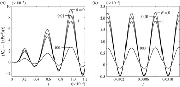
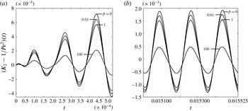
, 1 and 2. But, from the figures 23 and 24, it is observed that in small time, the amplitude of fluctuations of
 $K_{2}$
increases periodically with double frequency at first cycle for
 ${\it\alpha}=6$
and at first two cycles of oscillation for
 ${\it\alpha}=10$
. The double frequency period was also observed by Mazumder & Das (Reference Mazumder and Das1992) for Newtonian fluid. For
 ${\it\alpha}=4$
, very small double frequency period is seen in small time at first cycle of oscillation (see figure 22). So, double frequency period can be seen in the oscillation of
 $K_{2}$
at small time for large values of
 ${\it\alpha}$
(
 ${\geqslant}\,4$
) and becomes more frequent with the increase in
 ${\it\alpha}$
. From the figures 15–25, it is noticed that as
 ${\it\alpha}$
increases, the period of oscillations become shorter and the critical time for
 $K_{2}$
to reach a stationary state decreases.
Variation of dispersion coefficient
 $(K_{2}-1/Pe^{2})(t)$
with
 $t$
for different values of
 ${\it\beta}$
when
 ${\it\tau}_{y}=0.05$
,
 ${\it\alpha}=6$
,
 $e=0.5$
and
 $Sc=1000$
. (a) For small times; (b) for large times.

Variation of dispersion coefficient
 $(K_{2}-1/Pe^{2})(t)$
with
 $t$
for different values of
 ${\it\beta}$
when
 ${\it\tau}_{y}=0.05$
,
 ${\it\alpha}=10$
,
 $e=0.5$
and
 $Sc=1000$
. (a) For small times; (b) for large times.

Variation of dispersion coefficient
 $(K_{2}-1/Pe^{2})(t)$
with
 $t$
for different values of
 ${\it\beta}$
in small and large time when
 ${\it\tau}_{y}=0.05$
,
 ${\it\alpha}=0.1$
,
 $e=0.5$
and
 $Sc=1000$
.

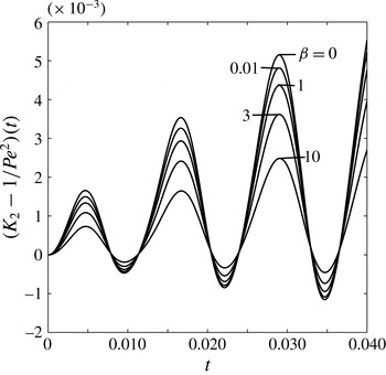
From the figures 22 and 26, it is evident that for
 ${\it\alpha}=4$
,
 $K_{2}$
becomes both positive and negative during the period of oscillation. It is worth mentioning that Nagarani & Sebastian (Reference Nagarani and Sebastian2013) have not been able to notice this in their study, (see the figure 4 of Nagarani & Sebastian (Reference Nagarani and Sebastian2013)). This could be due to the error associated with the numerical integration of their equation (32) for finding
 $K_{2}$
. This figure is reproduced in this work for the same set of parameter values and is shown in figure 26. Also, the expression given for
 $K_{1}$
is erroneous. In fact, the perturbation solution that was presented in Nagarani & Sebastian (Reference Nagarani and Sebastian2013) is valid only for small values of the Womersley frequency parameter
 ${\it\alpha}<1$
, but they have considered the values as large as 4, which is not acceptable.
Variation of dispersion coefficient
 $(K_{2}-1/Pe^{2})(t)$
with
 $t$
for different values of
 ${\it\tau}_{y}$
when
 ${\it\beta}=0$
,
 ${\it\alpha}=4$
,
 $e=0.5$
and
 $Sc=1000$
. (a) For small times; (b) for large times.

Limiting to smaller values of Womersley frequency parameter
 ${\it\alpha}<1$
, Sebastian & Nagarani (Reference Sebastian and Nagarani2015) studied the effect of wall absorption on the solute dispersion in pulsatile Casson fluid flow numerically using the Crank–Nicolson method adopted at each time step. The present investigation is a thorough analytical study considering the small and large values of Womersley frequency parameter
 ${\it\alpha}$
along with the effects of
 ${\it\tau}_{y}$
,
 $e$
and
 ${\it\beta}$
on both the convective coefficient
 $K_{1}$
and the dispersion coefficient
 $K_{2}$
and the present results are discussed already earlier in this paper. By considering the same set of parameters, we have re-examined the results that were presented in Sebastian & Nagarani (Reference Sebastian and Nagarani2015). Our results for small values of
 ${\it\alpha}$
are shown in figures 27–30. Comparison of the two calculations for the dispersion coefficient against the Womersley frequency parameter
 ${\it\alpha}$
between Sebastian & Nagarani (Reference Sebastian and Nagarani2015) and the present work revealed the following discrepancies.
Variation of dispersion coefficient
 $(K_{2}-1/Pe^{2})(t)$
with
 $t$
for different values of
 ${\it\tau}_{y}$
when
 ${\it\beta}=1$
,
 ${\it\alpha}=0.1$
,
 $e=0.1$
and
 $Sc=1000$
.

Variation of dispersion coefficient
 $(K_{2}-1/Pe^{2})(t)$
with
 $t$
for different values of
 $e$
when
 ${\it\tau}_{y}=0.02$
,
 ${\it\beta}=1$
,
 ${\it\alpha}=0.1$
and
 $Sc=1000$
.

Variation of dispersion coefficient
 $(K_{2}-1/Pe^{2})(t)$
with
 $t$
for different values of
 ${\it\beta}$
when
 ${\it\tau}_{y}=0.05$
,
 ${\it\alpha}=0.1$
,
 $e=0.2$
and
 $Sc=1000$
.

Variation of dispersion coefficient
 $(K_{2}-1/Pe^{2})(t)$
with
 $t$
for different values of
 ${\it\alpha}$
when
 ${\it\tau}_{y}=0.05$
,
 ${\it\beta}=1$
,
 $e=0.2$
and
 $Sc=1000$
.

It is seen from the figure (a) of Sebastian & Nagarani (Reference Sebastian and Nagarani2015) that
 $K_{2}$
becomes negative at large time
 $t=1$
for
 ${\it\tau}_{y}=0.1$
, but the present investigation shows that dispersion coefficient is non-negative for those chosen values of the parameters (see figure 27). Similarly, as
 ${\it\beta}$
increases in its range,
 $K_{2}$
is shown to decrease and become negative (see figure (c) of Sebastian & Nagarani (Reference Sebastian and Nagarani2015)). But it is noticed from the present investigation that as
 ${\it\beta}$
increases,
 $K_{2}$
decreases but does not become negative for
 ${\it\beta}=1$
at large time
 $t=1$
and this decrement of
 $K_{2}$
is small for small values of
 ${\it\beta}$
as shown in figure 29. The reason for decrement of dispersion coefficient has been discussed earlier in this study. Similar discrepancy is noticed for the dispersion coefficient
 $K_{2}$
when plotted against
 ${\it\alpha}$
, which are shown in figure (d) of Sebastian & Nagarani (Reference Sebastian and Nagarani2015) and figure 30 of the present investigation. The period of oscillation becomes shorter and
 $K_{2}$
reaches early a non-transient state as
 ${\it\alpha}$
increases. It is seen that for
 ${\it\alpha}=0.2$
, the amplitude of oscillations of
 $K_{2}$
becomes stable after four cycles of oscillation. But figure (d) of Sebastian & Nagarani (Reference Sebastian and Nagarani2015) indicated that
 $K_{2}$
decreases sharply at large time for
 ${\it\alpha}=0.2$
and does not reach a stationary state at large time
 $(0.5<t<1)$
. Figure 25 also shows that
 $K_{2}$
is positive for small value of
 ${\it\alpha}$
(say 0.1). This result is shown in three cycles of oscillation. As time increases, the amplitude of oscillations of
 $K_{2}$
increases and becomes stable at large time after first cycle of oscillation. All these above mentioned discrepancies are probably associated with the numerical treatment made in Sebastian & Nagarani (Reference Sebastian and Nagarani2015). Also, by considering
 ${\it\tau}_{y}=0$
(Newtonian fluid case), the variation of
 $K_{2}$
with small time
 $t$
for different values of
 ${\it\beta}$
and
 $e=1.5$
has been shown in figure 31. These results coincide exactly with those presented in figure 10 of Mazumder & Das (Reference Mazumder and Das1992) for all values of
 ${\it\beta}$
. To make this comparison, we set
 ${\it\alpha}$
as
 ${\it\omega}R^{2}/({\it\mu}/{\it\rho})$
instead of
 ${\it\alpha}^{2}$
which is used throughout this investigation. This comparison also shows that the present results are consistent for small and large times.
Variation of dispersion coefficient
 $(K_{2}-1/Pe^{2})(t)$
for different values of
 ${\it\beta}$
with small time
 $t$
when
 ${\it\tau}_{y}=0$
,
 $e=1.5$
,
 ${\it\alpha}=0.5$
and
 $Sc=1000$
.

Variation of dispersion coefficient
 $(K_{2}-1/Pe^{2})(t)$
for different values of
 ${\it\tau}_{y}$
with wall absorption parameter
 ${\it\beta}$
at large time
 $t=1$
when
 $e=0$
.

Variation of axial mean concentration
 $C_{m}(t,z)$
with axial distances
 $z$
for different values of
 ${\it\tau}_{y}$
when
 ${\it\beta}=0.01$
,
 $t=0.2$
,
 ${\it\alpha}=0.5$
,
 $e=0.5$
and
 $Sc=1000$
.

Yet other comparison of the present results is made with Sankarasubramanian & Gill (Reference Sankarasubramanian and Gill1973) (see figure 4) and Nagarani et al. (Reference Nagarani, Sarojamma and Jayaraman2004) (see figure 4a), which are in the best agreement, for the variation of axial dispersion coefficient
 $K_{2}$
with
 ${\it\beta}$
for different values of
 ${\it\tau}_{y}$
when
 $e=0$
and time
 $t$
is very large and is shown in figure 32. As
 ${\it\beta}$
increases,
 $K_{2}$
decreases and it also decreases as
 ${\it\tau}_{y}$
increases. The physical reason for this behaviour is discussed already earlier in this paper. This comparison also reveals that the present results are reliable.
4.4 Mean concentration
$C_{m}(t,z)$

The axial distribution of mean concentration
 $C_{m}$
depends on the time
 $t$
, yield stress
 ${\it\tau}_{y}$
, absorption parameter
 ${\it\beta}$
, amplitude of the fluctuating pressure component
 $e$
and frequency parameter
 ${\it\alpha}$
. In this study, the effects of
 $t$
,
 ${\it\tau}_{y}$
,
 ${\it\beta}$
,
 $e$
and
 ${\it\alpha}$
on the axial distribution of mean concentration have been analysed. The equation (3.7) involving exchange coefficient
 $K_{0}$
, convection coefficient
 $K_{1}$
and dispersion coefficient
 $K_{2}$
is solved to obtain the mean concentration
 $C_{m}$
. From (3.47) and (3.48a–c
),
 $C_{m}$
is obtained and it directly depends on
 $K_{0}$
,
 $K_{1}$
and
 $K_{2}$
.
The distribution profiles of mean concentration
 $C_{m}$
along the axial distance
 $z$
with different
 ${\it\tau}_{y}$
have been shown in figure 33. The increase in the non-Newtonian nature of the fluid is seen to have increasing value of the mean concentration. It is seen that as
 ${\it\tau}_{y}$
increases, the peak of mean concentration increases. Due to increase in yield stress of the fluid, flow velocity decreases and hence decreases the solute dispersion. Therefore, the mean concentration of solute increases in the axial direction. Figure 34 shows the distribution of mean concentration along the axial distance
 $z$
at different times
 $t$
. It is noticed that as
 $t$
increases, the peak of mean concentration decreases. Due to the presence of the boundary absorption at the tube wall, the solute in the system is continuously depleted and more amount of solute from the system is absorbed with the increasing of time
 $t$
. So, the solute concentration decreases as time increases. At small time after the injection of solute in the system, solute dispersion is controlled by convection and the molecular diffusion is not quite effective. Hence, the distribution profile of mean concentration at small time
 $(t=0.1)$
is more peaky. As the time increases, the dispersion becomes diffusion controlled at large time
 $(t=0.3)$
and the concentration profile becomes more blunt and dispersed. From figure 35, it is noticed that as
 ${\it\beta}$
increases, the peak of mean concentration decreases along the axial distance
 $z$
. Due to increase in
 ${\it\beta}$
, more amount of solute is supplied to conduct the boundary absorption or reaction at the tube wall and it reduces the concentration in the tube. From figure 36, it is observed that the peak of
 $C_{m}$
decreases as
 $e$
increases. As
 $e$
increases, both the flow velocity and the dispersion coefficient increases. Hence it decreases the solute concentration. But the decrement of
 $C_{m}$
is very small and it can be neglected. Figure 37 shows the axial distribution of mean concentration along the axial distance
 $z$
with different values of
 ${\it\alpha}$
. It is seen that the peak of
 $C_{m}$
increases with
 ${\it\alpha}$
but this increment is also very very small and it can be neglected.
Variation of axial mean concentration
 $C_{m}(t,z)$
with axial distances
 $z$
for different values of time
 $t$
when
 ${\it\tau}_{y}=0.05$
,
 ${\it\beta}=0.01$
,
 ${\it\alpha}=0.5$
,
 $e=0.5$
and
 $Sc=1000$
.

Variation of axial mean concentration
 $C_{m}(t,z)$
with axial distances
 $z$
for different values of
 ${\it\beta}$
when
 $t=0.2$
,
 ${\it\alpha}=0.5$
,
 ${\it\tau}_{y}=0.05$
,
 $e=0.5$
and
 $Sc=1000$
.

Variation of axial mean concentration
 $C_{m}(t,z)$
with axial distances
 $z$
for different values of
 $e$
when
 $t=0.2$
,
 ${\it\beta}=0.01$
,
 ${\it\alpha}=0.5$
,
 ${\it\tau}_{y}=0.05$
and
 $Sc=1000$
.

Variation of axial mean concentration
 $C_{m}(t,z)$
with axial distances
 $z$
for different values of
 ${\it\alpha}$
when
 $t=0.2$
,
 ${\it\beta}=0.01$
,
 $e=0.5$
,
 ${\it\tau}_{y}=0.05$
and
 $Sc=1000$
.

When
 $e=0$
and
 $t$
is very large, the distribution profiles of mean concentration
 $C_{m}$
at
 $z=0.5$
with
 $t$
for various values of
 ${\it\beta}$
and
 ${\it\tau}_{y}$
are presented in figure 38. It is observed that as
 ${\it\beta}$
increases, the peak of
 $C_{m}$
decreases as also seen in Nagarani et al. (Reference Nagarani, Sarojamma and Jayaraman2004). The mean concentration
 $C_{m}$
decreases with the time due to constant depletion of solute occurring at the tube wall. These results are found to be in agreement with Sankarasubramanian & Gill (Reference Sankarasubramanian and Gill1973) for
 ${\it\tau}_{y}=0$
and Nagarani et al. (Reference Nagarani, Sarojamma and Jayaraman2004).
Variation of axial mean concentration
 $C_{m}(t,z)$
with time
 $t$
for different values of
 ${\it\tau}_{y}$
and
 ${\it\beta}$
at large time
 $t=1$
when
 $e=0$
and
 $z=0.5$
.

5 Conclusions
In this analysis, the effect of catalytic reaction at the tube wall on axial dispersion of solute in a periodic flow of Casson fluid is discussed with the pulsatile pressure gradient by applying the generalized dispersion model. The three effective transport coefficients i.e. exchange, convective and dispersion coefficients are determined to analyse the axial dispersion and axial mean concentration of solute in the presence of the boundary absorption at the tube wall. It is observed that exchange coefficient
 $K_{0}$
depends on time
 $t$
and wall absorption parameter
 ${\it\beta}$
but the convective coefficient
 $K_{1}$
and dispersion coefficient
 $K_{2}$
depend on time
 $t$
, wall absorption parameter
 ${\it\beta}$
, yield stress of the fluid
 ${\it\tau}_{y}$
, the fluctuating pressure component
 $e$
and Womersley frequency parameter
 ${\it\alpha}$
. The results of
 $K_{0}$
,
 $K_{1}$
,
 $K_{2}$
and
 $C_{m}$
for a Newtonian fluid at large time are found to be in best agreement with Sankarasubramanian & Gill (Reference Sankarasubramanian and Gill1973) and Nagarani et al. (Reference Nagarani, Sarojamma and Jayaraman2004). As
 ${\it\tau}_{y}$
increases, the amplitude of fluctuations and the magnitude of both negative convective coefficient
 $-K_{1}$
and dispersion coefficient
 $K_{2}$
decreases. In this study, it is seen that the amplitude of fluctuations of both
 $-K_{1}$
and
 $K_{2}$
increases with
 $e$
. As
 ${\it\beta}$
increases,
 $K_{1}$
and
 $K_{2}$
increases and decreases, respectively. As
 ${\it\alpha}$
increases, the amplitude of oscillations of
 $K_{2}$
decreases. At small time,
 $K_{2}$
increases cyclically with the period of oscillation and becomes stable at large time. It is observed that the critical time for which
 $K_{2}$
reaches a non-transient state is independent of
 ${\it\tau}_{y}$
and
 $e$
of the fluid but dependent of
 ${\it\alpha}$
. For small
 ${\it\alpha}$
,
 $K_{2}$
oscillates with single frequency period at small time but for large
 ${\it\alpha}$
, it begins to oscillate at small time with double frequency period. As
 ${\it\alpha}$
increases,
 $K_{2}$
fluctuates in shorter period of oscillation. For large values of
 ${\it\alpha}$
,
 $K_{2}$
becomes positive and negative during the cycle of oscillation and this phenomena also depends on
 ${\it\tau}_{y}$
,
 $e$
and
 ${\it\beta}$
. The peak of axial mean concentration
 $C_{m}$
increases with
 ${\it\tau}_{y}$
. As the time
 $t$
increases after the injection of solute, the peak of
 $C_{m}$
decreases and becomes flat. It is also seen that the peak of
 $C_{m}$
decreases with increment of
 ${\it\beta}$
. For the variation of
 $e$
and
 ${\it\alpha}$
, there is not significant change in axial distribution of mean concentration
 $C_{m}$
and it can be neglected.
Acknowledgements
The authors are thankful to all the reviewers for their valuable comments and constructive criticism for the improvement of the technical content of the manuscript.