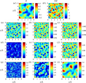
1. Introduction
Near-inertial waves (NIWs) are ubiquitous in the ocean. They contribute strongly to surface mixing, and hence to biological activity, (e.g. Granata, Wiggert & Dickey Reference Granata, Wiggert and Dickey1995). They also propagate to depth where they eventually dissipate, thus participating in deep vertical mixing and the global overturning circulation (Ferrari & Wunsch Reference Ferrari and Wunsch2009). The propagation of NIWs in heterogeneous flows has motivated a great deal of work. One of the main conclusions, emerging from both numerical simulations (Lee & Niiler Reference Lee and Niiler1998; Zhai, Greatbach & Zhao Reference Zhai, Greatbach and Zhao2005; Danioux, Klein & Rivière Reference Danioux, Klein and Rivière2008) and observational data (Kunze & Sanford Reference Kunze and Sanford1984; Elipot, Lumpkin & Prieto Reference Elipot, Lumpkin and Prieto2010; Joyce et al. Reference Joyce, Toole, Klein and Thomas2013), is that near-inertial energy concentrates in anticyclones, i.e. in regions of negative relative vorticity in the Northern Hemisphere and positive relative vorticity in the Southern Hemisphere.
Various explanations have been advanced for this phenomenon. Using a Wentzel–Kramers–Brillouin (WKB) approach, Kunze (Reference Kunze1985) showed that refraction by a background flow leads to an ‘effective’ inertial frequency
 $f_{e}$
shifted from the local Coriolis frequency
 $f$
by
 ${\it\zeta}/2$
, where
 ${\it\zeta}$
is the local relative vorticity:
 $f_{e}=f+{\it\zeta}/2$
. Because the range of allowed wave frequencies
 ${\it\omega}$
satisfies
 $|\,f_{e}|<{\it\omega}<N$
, where
 $N$
is the stratification frequency (usually much larger than
 $|\,f|$
), it is larger in regions of negative vorticity in the Northern Hemisphere. Therefore, anticyclonic regions are expected to be more energetic because (i) NIWs propagating poleward can enter regions of negative vorticity, but not regions of positive vorticity, and (ii) frequencies lower than
 $f$
present in the forcing can become resonant (Kunze Reference Kunze1985). This explanation is subject to caution, however, because the initial length scales of NIWs, set by atmospheric storms, are typically much larger than the length scales of geostrophic flows (the ratio of tropospheric to oceanic radii of deformation is approximately 10), thus invalidating the assumption underlying the WKB approximation.
Alternative explanations were offered by Young & Ben Jelloul (Reference Young and Ben Jelloul1997) and Klein, Llewellyn Smith & Lapeyre (Reference Klein, Llewellyn Smith and Lapeyre2004). These rely on the NIW model developed by Young & Ben Jelloul (Reference Young and Ben Jelloul1997), hereafter referred to as the YBJ model, which exploits the small frequency spread of NIWs near
 $f$
and makes no assumption about their spatial scales. These explanations rely on strong assumptions: strong dispersion for Young & Ben Jelloul (Reference Young and Ben Jelloul1997), short time and restrictions on the spectrum of the vorticity field for Klein et al. (Reference Klein, Llewellyn Smith and Lapeyre2004) In this paper, we revisit the issue and, taking the YBJ model as a starting point, show that a so-far overlooked conservation law provides a robust argument for the concentration of NIWs in anticyclones. Section 2 derives the conservation law in the simple case of a reduced-gravity shallow-water model, the YBJ approximation of which is obtained in appendix A. (The extension to a continuously stratified fluid is straightforward when the background flow is assumed to be barotropic, so that NIWs can be expanded in vertical modes.) Section 3 demonstrates analytically and numerically how NIW concentration in anticyclones stems from the conservation law. Some conclusions and perspectives are offered in § 4.
2. Model and conservation laws
2.1. The YBJ model and analogy with the Schrödinger equation
We study the propagation of NIWs in a steady geostrophic flow with a reduced-gravity shallow-water model (e.g. Cushman-Roisin Reference Cushman-Roisin1994). This slab model can be thought of as representing the dynamics of NIWs confined in a mixed layer capping an abyssal layer where the only motion is the imposed geostrophic flow, assumed to be identical in both layers. For NIWs, the horizontal velocity
 $(u,v)$
can be written in terms of a complex amplitude
 $M$
according to
 $u+\text{i}v=M\text{e}^{-\text{i}ft}$
. The slow (compared with
 $f^{-1}$
) time evolution of
 $M$
is governed by the YBJ equation
 $$\begin{eqnarray}\partial _{t}M+J({\it\psi},M)-\text{i}\frac{h}{2}{\rm\Delta}M+\text{i}\frac{{\rm\Delta}{\it\psi}}{2}M=0,\end{eqnarray}$$
where
 ${\it\psi}$
and
 ${\rm\Delta}{\it\psi}$
are the streamfunction and vorticity of the steady geostrophic flow,
 $J$
is the horizontal Jacobian and
 $h=g^{\prime }H/f$
is a dispersion parameter, with
 $g^{\prime }$
and
 $H$
the reduced gravity and average depth of the mixed layer. We assume that
 $h>0$
, as in the Northern Hemisphere where
 $f>0$
. The respective terms quantify the effects due to advection, dispersion and refraction. A concise derivation of (2.1) is given in appendix A.
Two simple facts help in understanding the dynamics of (2.1). First, for any constant
 ${\it\alpha}>0$
the YBJ equation is invariant under the scaling transformation
 ${\it\psi}\mapsto {\it\alpha}{\it\psi}$
,
 $h\mapsto {\it\alpha}h$
,
 $t\mapsto t/{\it\alpha}$
. This makes it obvious that the intrinsic dynamics of (2.1) depends only on the single non-dimensional parameter
 $h/{\it\Psi}$
, say, where
 ${\it\Psi}$
is the amplitude scale of
 ${\it\psi}$
.
Second, without the advection term
 $J({\it\psi},M)$
the YBJ equation is identical to the Schrödinger equation that governs the complex wavefunction
 ${\it\phi}(x,y,t)$
for a single particle with unit mass and external potential
 $V(x,y)$
:
 $$\begin{eqnarray}\partial _{t}{\it\phi}-\text{i}\frac{\hbar}{2}{\rm\Delta}{\it\phi}+\text{i}\frac{V}{\hbar}{\it\phi}=0.\end{eqnarray}$$
Here,
 $\hbar$
is Planck’s constant divided by
 $2{\rm\pi}$
. Comparing (2.1) and (2.2) and identifying
 $\hbar$
with
 $h$
shows that the effective potential in (2.1) is
 $$\begin{eqnarray}V=h\frac{{\rm\Delta}{\it\psi}}{2}.\end{eqnarray}$$
Clearly, regions of higher
 $V$
repel the particle whereas regions of lower
 $V$
attract it. Hence, if the advection term is negligible, then the mathematical analogy between the particle probability density
 $|{\it\phi}|^{2}$
and the inertial wave kinetic energy density
 $|M|^{2}$
readily implies that cyclones repel inertial waves while anticyclones attract them (Balmforth, Llewellyn Smith & Young Reference Balmforth, Llewellyn Smith and Young1998). For the special case of an axisymmetric anticyclonic vortex, this is confirmed by the existence of axisymmetric trapped modes (Llewellyn Smith Reference Llewellyn Smith1999).
Of course, if the advection term cannot be neglected then the simple analogy with the Schrödinger equation breaks down. Hence, the main task is to understand how the advection term alters the basic Schrödinger dynamics as a function of
 $h/{\it\Psi}$
. For this it becomes crucial to study the full set of conservation laws associated with (2.1), as we shall do now.
2.2. Conservation laws
By multiplying (2.1) by
 $M^{\ast }$
and adding its complex conjugate we obtain
 $$\begin{eqnarray}\partial _{t}{\textstyle \frac{1}{2}}|M|^{2}+J\left({\it\psi},{\textstyle \frac{1}{2}}|M|^{2}\right)+\boldsymbol{{\rm\nabla}}\boldsymbol{\cdot }\boldsymbol{F}=0,\end{eqnarray}$$
where
 $\boldsymbol{F}=\text{i}h(M\boldsymbol{{\rm\nabla}}M^{\ast }-M^{\ast }\boldsymbol{{\rm\nabla}}M)/4$
. In a finite domain with suitable boundary conditions (periodicity or
 $M=0$
), integration of (2.4) gives the conservation of NIW kinetic energy, as derived by Young & Ben Jelloul (Reference Young and Ben Jelloul1997),
 $$\begin{eqnarray}\frac{\text{d}}{\text{d}t}\iint \frac{1}{2}|M|^{2}\,\text{d}x\,\text{d}y=0.\end{eqnarray}$$
There is another conservation law associated with (2.1) and not mentioned in Young & Ben Jelloul (Reference Young and Ben Jelloul1997). It is derived by forming the combination
 $M_{t}^{\ast }(2.1)-M_{t}(2.1)^{\ast }$
and integrating the result over the domain. Using properties of the Jacobian and integrating by parts, this gives
 $$\begin{eqnarray}\frac{\text{d}}{\text{d}t}(I_{1}+I_{2}+I_{3})=0,\end{eqnarray}$$
where
 $$\begin{eqnarray}I_{1}=\iint \text{i}h{\it\psi}J(M^{\ast },M)\,\text{d}x\,\text{d}y,\quad I_{2}=\iint \frac{h^{2}}{2}|\boldsymbol{{\rm\nabla}}M|^{2}\,\text{d}x\,\text{d}y,\quad I_{3}=\iint h\frac{{\rm\Delta}{\it\psi}}{2}|M|^{2}\,\text{d}x\,\text{d}y.\end{eqnarray}$$
The terms
 $I_{1}$
,
 $I_{2}$
and
 $I_{3}$
stem directly from the advection, dispersion and refraction terms in the YBJ equation. The overall factors of
 $h$
are included for two practical reasons: to keep the values of the invariants comparable when
 $h$
is varied and to highlight the appearance of the effective potential
 $V$
from (2.3) in
 $I_{3}$
. The consequences of the new conservation law (2.6) are discussed in more detail in the next section. In the absence of a geostrophic flow,
 $I_{1}$
and
 $I_{3}$
are identically zero, and
 $I_{2}$
can be recognized as the scaled NIW potential energy averaged over the fast time scale. This is not unexpected, as explained in appendix B. In the presence of a steady flow,
 $I_{1}+I_{2}+I_{3}$
can be interpreted as an energy in that its conservation is associated with the time invariance of (2.1). Unlike (2.5),
 $I_{1}+I_{2}+I_{3}$
is not conserved for arbitrary time-dependent flows. However, when the flow and NIWs evolve in a dynamically consistent manner, an analogous conservation law holds that accounts for energy transfers between the flow and the NIWs (Xie & Vanneste Reference Xie and Vanneste2015).
We remark that, in a steady geostrophic flow, differentiation of (2.1) with respect to time shows that
 $M_{t}$
satisfies the same equation as
 $M$
, and hence the same conservation laws. In particular,
 $$\begin{eqnarray}\frac{\text{d}}{\text{d}t}\iint \frac{1}{2}|M_{t}|^{2}\,\text{d}x\,\text{d}y=0\end{eqnarray}$$
means that no stationary state can be reached.
3. Near-inertial-wave concentration in anticyclones
Non-dimensionalization of (2.1) using
 $x=Lx^{\prime }$
,
 ${\it\psi}={\it\Psi}{\it\psi}^{\prime }$
,
 $h={\it\Psi}h^{\prime }$
and
 $t=(L^{2}/{\it\Psi})t^{\prime }$
, with
 $L$
the typical length scale of the geostrophic flow, gives an identical equation for the primed variables. Again, this makes it obvious that
 $h^{\prime }=h/{\it\Psi}$
is the only relevant parameter; in § 3.3 we conduct simulations with different values of
 $h/{\it\Psi}$
. This parameter is the reduced-gravity shallow-water equivalent of the parameter
 ${\it\Upsilon}={\it\Psi}/h=1/h^{\prime }$
used in Young & Ben Jelloul (Reference Young and Ben Jelloul1997) and Balmforth et al. (Reference Balmforth, Llewellyn Smith and Young1998), on which they base their ‘strong-dispersion’ (
 $h/{\it\Psi}\gg 1$
) and ‘strong-trapping’ (or ‘strong-advection’,
 $h/{\it\Psi}\ll 1$
) approximations. In the ocean,
 $h/{\it\Psi}$
is highly variable because of varying kinetic energy levels and stratification. For instance, typical values for the North Atlantic might be
 $f=10^{-4}~\text{s}^{-1}$
,
 $g^{\prime }=2\times 10^{-3}~\text{m}~\text{s}^{-2}$
,
 $L=50~\text{km}$
; taking
 $H$
and
 $U$
in the ranges
 $H\in [50,100]~\text{m}$
,
 $U\in [0.005,0.1]~\text{m}~\text{s}^{-1}$
gives
 $h/{\it\Psi}\in [0.2,8]$
.
We will consider a specific initial-value problem in which
 $M(x,y,0)=1$
. Without loss of generality this represents an eastward NIW momentum deposition by a storm: because storm scales are typically much larger than ocean eddy scales, a homogeneous initial condition for
 $M$
is appropriate.
The conservation law (2.6) involves
 $I_{3}$
, which is proportional to the covariance between
 $|M|^{2}$
and
 ${\rm\Delta}{\it\psi}$
; it is therefore relevant to the concentration of NIWs in anticyclones, which corresponds to
 $I_{3}<0$
. At
 $t=0$
,
 $I_{1}=I_{2}=I_{3}=0$
(assuming no net vorticity – a given with periodic boundary conditions). The development of spatial heterogeneities in the
 $M$
field must lead to an increase in the positive definite
 $I_{2}$
, which is then compensated by
 $I_{1}+I_{3}<0$
. Of course, if
 $I_{1}$
is negligible then
 $I_{3}$
must take negative values, but in the general case it is less clear whether
 $I_{3}$
behaves in this way. We next provide an asymptotic argument that
 $I_{3}$
becomes negative for all values of
 $h/{\it\Psi}$
at short times. This is followed by a long-time scaling argument for (2.1) as a function of
 $h/{\it\Psi}$
, which predicts that
 $I_{3}<0$
for large and intermediate values of
 $h/{\it\Psi}$
but not for small values of this parameter. These predictions are then checked against numerical simulations in § 3.3.
3.1. Short-time solution
With homogeneous initial conditions, the first physical effect on NIW propagation is due to refraction, and the short-time behaviour is
 $M(x,y,t)=\exp (-\text{i}t{\rm\Delta}{\it\psi}(x,y)/2)\equiv \bar{M}(x,y,t)$
(Danioux et al.
Reference Danioux, Klein and Rivière2008). A cautious definition for short time here is
 $t\ll t_{s}=1/\!\max \{{\it\Psi}/(2L^{2}),h/(2L^{2})\}$
. For such times, the solution can be sought as the expansion
 $M=\bar{M}+M^{\prime }$
, with
 $M^{\prime }(x,y,t=0)=0$
and
 $|M^{\prime }|\ll 1$
. Introducing this into (2.1) gives
 $$\begin{eqnarray}\partial _{t}M^{\prime }+J({\it\psi},M^{\prime })-\text{i}\frac{h}{2}{\rm\Delta}M^{\prime }+\text{i}\frac{{\rm\Delta}{\it\psi}}{2}M^{\prime }=-J({\it\psi},\bar{M})+\text{i}\frac{h}{2}{\rm\Delta}\bar{M}.\end{eqnarray}$$
Because of the form of
 $\bar{M}$
, the short-time behaviour of the right-hand side of (3.1) behaves as
 $O(t)$
, hence forcing
 $M^{\prime }(t)=O(t^{2})$
for small
 $t$
. Keeping this in mind, we now compare the relative size of terms
 $I_{1}$
and
 $I_{2}$
in (2.6). First, because
 $J(\bar{M}^{\ast },\bar{M})=0$
,
 $I_{1}$
is dominated by terms of the form
 $\text{i}h{\it\psi}J(\bar{M}^{\ast },M^{\prime })$
, resulting in an
 $O(t^{3})$
dependence. Second,
 $I_{2}$
is dominated by
 $h^{2}|\boldsymbol{{\rm\nabla}}\bar{M}|^{2}/2$
, yielding an
 $O(t^{2})$
dependence. Hence, for short enough times,
 $I_{2}\gg I_{1}$
. The NIW energy concentration in regions of negative vorticity can also be deduced from (2.4). On injecting the short-time solution
 $\bar{M}(x,y,t)$
into
 $\boldsymbol{F}$
, one finds that the amplitude of
 $M$
obeys
 $$\begin{eqnarray}\partial _{t}\frac{1}{2}|M|^{2}\simeq \frac{ht}{4}{\it\Delta}^{2}{\it\psi}\end{eqnarray}$$
at short times, consistent with the short-time solution of Klein et al. (Reference Klein, Llewellyn Smith and Lapeyre2004). Because the vorticity field and its Laplacian are anticorrelated, (3.2) gives an increase of NIW energy in anticyclonic regions for all values of
 $h/{\it\Psi}$
.
3.2. Long-time scaling arguments
For long times the spatial scales of
 $M$
need not be equal to those of
 ${\it\psi}$
anymore and hence the dominant balance between the various terms in (2.1) may shift accordingly. However, the conservation law (2.8) implies
 $$\begin{eqnarray}\iint \frac{1}{2}|M_{t}|^{2}\,\text{d}x\,\text{d}y=\iint \frac{1}{2}|M_{t}(t=0)|^{2}\,\text{d}x\,\text{d}y=\iint \frac{1}{2}({\rm\Delta}{\it\psi}/2)^{2}\,\text{d}x\,\text{d}y,\end{eqnarray}$$
and together with (2.5) this means that for all times the root-mean-square magnitudes of
 $M$
and
 $M_{t}$
scale with unity and
 ${\it\Psi}/L^{2}$
respectively. This allows a simple scaling analysis of the four terms in (2.1), which after rearranging yields
 $$\begin{eqnarray}1,\quad \frac{L}{l},\quad \frac{h}{{\it\Psi}}\frac{L^{2}}{l^{2}},\quad 1.\end{eqnarray}$$
Here,
 $l$
is the long-time spatial scale of
 $M$
such that
 $\boldsymbol{{\rm\nabla}}M=O(1/l)$
. We use (3.4) to determine how
 $l/L$
may depend on
 $h/{\it\Psi}$
. First, in the ‘strong-dispersion’ regime
 $h/{\it\Psi}\gg 1$
the only possible balance in (3.4) is
 $l/L=\sqrt{h/{\it\Psi}}$
, which balances dispersion and refraction whilst advection is negligible. As expected, this reduces the YBJ dynamics to that of the Schrödinger equation, so
 $I_{1}$
is negligible and
 $I_{3}\approx -I_{2}$
. In this regime the spatial scale of
 $M$
is larger than that of the background flow
 ${\it\psi}$
by a factor of
 $\sqrt{h/{\it\Psi}}$
.
Second, in the opposite regime
 $h/{\it\Psi}\ll 1$
one scaling possibility is
 $l=L$
, which balances advection and refraction whilst dispersion becomes negligible. However, from (2.1) this would correspond to an advective dynamics along streamlines in which
 $|M|$
is conserved while its phase continues to change by the refraction as in the short-term solution derived in § 3.1. This would inevitably lead to the generation of increasingly small spatial scales in
 $M$
and hence defeat the assumption
 $l=L$
. We must therefore look at the alternative, a balance between the advective and dispersive terms based on
 $l/L=h/{\it\Psi}$
. The advective and dispersive terms then provide a new leading-order dominant balance of size
 ${\it\Psi}/h\gg 1$
to the long-term evolution of the YBJ equation. Consequently, in this scenario the refraction is weak and
 $I_{3}$
becomes negligible, and so
 $I_{1}\approx -I_{2}$
. Moreover, the spatial scale of
 $M$
is much smaller than that of
 ${\it\psi}$
, by a factor of
 $h/{\it\Psi}$
.
It should be noted that this small horizontal scale may invalidate the assumption of small
 $h/(\,fl^{2})$
that underpins the near-inertial YBJ model (see appendix A). Using
 $l=hL/{\it\Psi}$
, we rewrite this assumption as
 ${\it\Psi}/(\,fL^{2})\ll h/{\it\Psi}$
in terms of the Rossby number on the left-hand side. Hence, for small but fixed
 $h/{\it\Psi}$
the near-inertial approximation holds provided that the Rossby number is small enough.
Finally, in the intermediate regime
 $h/{\it\Psi}=1$
the scaling
 $l/L=1$
makes all terms equally important. It stands to reason that in this intermediate regime
 $I_{3}$
will take moderate negative values, consistent with a monotonic transition between its value
 $I_{3}\approx 0$
for
 $h/{\it\Psi}\ll 1$
and its negative value
 $I_{3}\approx -I_{2}$
for
 $h/{\it\Psi}\gg 1$
. However, only in this intermediate regime does the length scale of
 $M$
equal that of
 ${\it\psi}$
, which arguably is the best situation for effective concentration of NIW energy in anticyclones. This suggests that the intermediate regime might be the most effective for this purpose. Of course, this simple scaling analysis can only provide a heuristic guide to the full NIW energy dynamics, not least because the spatial scales of
 $|M|^{2}$
are not related in a trivial way to those of
 $M$
. Still, we will see that the present scaling arguments do indeed provide a useful guide for understanding the numerical simulations.
3.3. Numerical simulations
Equation (2.1) is solved numerically on a doubly periodic
 $256\times 256$
grid using a pseudo-spectral time-split Euler scheme. A weak biharmonic dissipation is added for numerical stability. The streamfunction
 ${\it\psi}$
is taken as a single realization of a homogeneous isotropic Gaussian random process, with Gaussian correlation function and a correlation length
 $L$
of approximately
 $1/5$
of the domain size. The chosen vorticity field is shown in figure 1(
 $b^{\prime }$
). Because its correlation scale is much smaller than the size of the domain, the results presented here are generic. We run three simulations with the same background flow but different values of
 $h$
such that
 $h/{\it\Psi}=0.2$
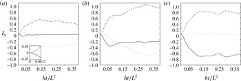
, 1 and 10, representative of the strong-advection, intermediate and strong-dispersion regimes. Simulations are stopped when the various terms in (2.6) no longer evolve significantly, which occurs at
 $t\simeq 0.3L^{2}/h$
(figure 2). For the intermediate case, using the values given at the beginning of this section, we find a time scale of between four and eight days, which is realistic.
Streamfunction (
 $a^{\prime }$
) and associated normalized vorticity field (
 $b^{\prime }$
) of the background flow, and evolution of the NIW amplitude
 $|M|$
for
 $h/{\it\Psi}=0.2$
(a,d,g),
 $h/{\it\Psi}=1$
(b,e,h) and
 $h/{\it\Psi}=10$
(c,f,i). Here, (a–c) correspond to very short times after the start of the simulations (
 $1/80$
th of the length of the simulations), (d–f) to short times (
 $1/16$
th of the length of the simulations) and (g–i) to the end of the simulations.

Snapshots of
 $|M|$
are shown in figure 1 for very short, short and long times for the three values of
 $h/{\it\Psi}$
. At very short times, for all values of
 $h$
,
 $|M|$
is clearly anticorrelated with the vorticity field (or correlated with its Laplacian), as predicted by (3.2). As time increases, the variance of
 $|M|$
increases, substantially for small
 $h/{\it\Psi}$
but much less for large
 $h/{\it\Psi}$
. This is consistent with the scaling
 $|M-1|=O({\it\Psi}/h)$
that holds for short time and arbitrary
 $h/{\it\Psi}$
(as follows from integrating (3.2) for
 $t\lesssim L^{2}/h$
) and for all time and large
 $h/{\it\Psi}$
(as follows from a perturbative treatment of (2.1)). At the end of the simulation,
 $M$
has larger scales than at the very first instants for
 $h/{\it\Psi}=10$
, in accordance with the scaling arguments in § 3.2 and also with the ‘truncated Laplacian’ solution of Klein et al. (Reference Klein, Llewellyn Smith and Lapeyre2004). The spectrum of
 $M$
does not change much afterwards (not shown), in contrast to the theory of Klein et al. (Reference Klein, Llewellyn Smith and Lapeyre2004) which predicts a continued cascade towards large scales. As expected, the evolution is very different for
 $h/{\it\Psi}=0.2$
. The short-time solution (figure 1
d) is consistent with a passive-scalar-type scenario: after the initial generation of spatial scales in
 $|M|$
(figure 1
a), the
 $|M|$
field is stretched and folded, while its amplitude grows due to dispersion. Later on (figure 1
g), NIW scales much smaller than the flow scales develop, consistent with § 3.2.
The behaviour of
 $|M|$
is reflected in the evolution of
 $I_{1}$
,
 $I_{2}$
and
 $I_{3}$
displayed in figure 2. The generation of small scales by refraction subsequently modulated by dispersion leads to an increase of
 $I_{2}$
. This is balanced by the decrease of
 $I_{3}$
at short times for all values of
 $h/{\it\Psi}$
and for all times for
 $h/{\it\Psi}=10$
, as predicted by our scaling argument. Conversely, for
 $h/{\it\Psi}=0.2$
we obtain
 $I_{1}\simeq -I_{2}$
, indicative of the balance between advection and dispersion noted above (in this case, the amplitude of these quantities decreases slightly in time because of numerical dissipation). For
 $h/{\it\Psi}=1$
, all terms
 $I_{1}$
,
 $I_{2}$
and
 $I_{3}$
have similar final amplitudes. It should be noted that the amplitude of
 $I_{2}$
is roughly the same in the three simulations. From the scaling
 $|M-1|=O({\it\Psi}/h)$
mentioned above, we infer that
 $I_{2}$
is proportional to
 ${\it\Psi}^{2}/L^{2}$
, and similarly for
 $I_{3}$
. This justifies a posteriori the inclusion of the overall factor
 $h$
in the definition of
 $I_{1}$
,
 $I_{2}$
and
 $I_{3}$
.
Evolution of the integrals
 $I_{1}$
(dotted line),
 $I_{2}$
(dashed line) and
 $I_{3}$
(thin solid line) in (2.6) for
 $h/{\it\Psi}=0.2$
(a), 1 (b) and 10 (c). Here,
 $I_{1}$
,
 $I_{2}$
and
 $I_{3}$
are scaled by the area of the domain. The inset in (a) represents a zoom on very short times.

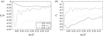
We now turn to the concentration of NIW energy in anticyclones. This is best quantified by
 $I_{3}/h$
, that is, the covariance between
 ${\rm\Delta}{\it\psi}/2$
and
 $|M|^{2}$
. An alternative diagnostic is the correlation between
 $|M|^{2}$
and
 ${\rm\Delta}{\it\psi}/2$
, namely
 $$\begin{eqnarray}C=\frac{I_{3}}{h\left(\displaystyle {\it\sigma}_{M}^{2}\iint ({\rm\Delta}{\it\psi}/2)^{2}\,\text{d}x\,\text{d}y\right)^{1/2}},\quad \text{where}~{\it\sigma}_{M}^{2}=\iint (|M|^{4}-1)\,\text{d}x\,\text{d}y\end{eqnarray}$$
is the variance of the NIW energy. We emphasize that
 $C$
focuses on the match between the spatial patterns of NIW energy and vorticity irrespective of their amplitudes; the more intuitive colocation of high values of NIW energy with regions of anticyclonic vorticity is measured by
 $I_{3}/h$
. The evolution of both
 $I_{3}/h$
and
 $C$
is shown for the three values of
 $h/{\it\Psi}$
in figure 3. At the end of the simulations, the covariance
 $I_{3}/h$
is largest for intermediate values of
 $h/{\it\Psi}$
. Small values of
 $h/{\it\Psi}$
lead to a strongly heterogeneous
 $|M|^{2}$
(large
 ${\it\sigma}_{M}^{2}$
, as seen in figure 1
g) but relatively weak correlation of
 $|M|^{2}$
and
 ${\rm\Delta}{\it\psi}$
(figure 3
b, dashed line); conversely, large values of
 $h/{\it\Psi}$
lead to a strong correlation (figure 3
b, solid line) but weak heterogeneity of
 $|M|^{2}$
. The intermediate case displays both a relatively strong
 ${\it\sigma}_{M}^{2}$
(figure 1
h) and a strong correlation (figure 3
b, dotted line), giving the maximum covariance.
(a) Spatial covariance
 $I_{3}/h$
and (b) correlation
 $C$
between
 $|M|^{2}$
and
 ${\rm\Delta}{\it\psi}/2$
for
 $h/{\it\Psi}=0.2$
, 1 and 10. Legend in (a) applies also to (b).

4. Discussion
The results described in this paper in the context of the reduced-gravity shallow-water system demonstrate that the development of spatial heterogeneity in a homogeneous field of NIWs due to the interaction with the barotropic vorticity field is inevitably accompanied by a concentration of NIW energy in anticyclones. We emphasize that this result does not make assumptions about the relative importance of dispersion (such as the strong-dispersion approximation of Young & Ben Jelloul Reference Young and Ben Jelloul1997 and Balmforth et al.
Reference Balmforth, Llewellyn Smith and Young1998) or the nature of the vorticity field and smallness of advection (Klein et al.
Reference Klein, Llewellyn Smith and Lapeyre2004). Instead, it arises as a consequence of a conservation law associated with the model of Young & Ben Jelloul (Reference Young and Ben Jelloul1997). Therefore, the concentration of NIW energy in anticyclones is a much more robust phenomenon than previously thought. In particular, it is the strongest for the intermediate regime
 $h/{\it\Psi}=O(1)$
, when refraction, dispersion and advection are all significant.
We note that (3.3) leads to an interesting conclusion for
 $h/{\it\Psi}\gg 1$
. In this limit,
 $M\rightarrow 1$
, as explained above, so that the refraction term in (2.1) becomes approximately
 $\text{i}{\rm\Delta}{\it\psi}/2$
. By (3.3) the time-derivative term has the same amplitude as the refraction term in (2.1), in contrast to previous treatments of the strong-dispersion limit which neglect it (Young & Ben Jelloul Reference Young and Ben Jelloul1997; Balmforth et al.
Reference Balmforth, Llewellyn Smith and Young1998). In this case, a more complete solution of (2.1) at short times is
 $$\begin{eqnarray}M=1+\frac{1}{h}\iint \hat{{\it\psi}}(\boldsymbol{k})\text{e}^{\text{i}\boldsymbol{k}\boldsymbol{\cdot }\boldsymbol{x}}(1-\text{e}^{-\text{i}h|\boldsymbol{k}|^{2}t/2})\,\text{d}\boldsymbol{k}+O(({\it\Psi}/h)^{^{2}}),\end{eqnarray}$$
where
 $\hat{{\it\psi}}(\boldsymbol{k})$
is the Fourier transform of the streamfunction
 ${\it\psi}$
at wavenumber
 $\boldsymbol{k}$
. From (4.1), the adjustment of the initial condition
 $M=1$
towards the ‘balanced state’ with
 $M=1+{\it\psi}/h+O(({\it\Psi}/h)^{2})$
is accompanied by the emission of
 $O({\it\Psi}/h)$
-amplitude waves. Although the latter part is missing from Young & Ben Jelloul (Reference Young and Ben Jelloul1997) and Balmforth et al. (Reference Balmforth, Llewellyn Smith and Young1998), (4.1) shows that the correlation between
 $|M|$
and
 ${\it\psi}$
(hence the anticorrelation between
 $|M|$
and the vorticity field) remains true on average. It should be noted that a slow modulation of (4.1) should be added to describe the long-time behaviour of
 $M$
(Young & Ben Jelloul Reference Young and Ben Jelloul1997).
In this paper, we make the strong assumption of a steady background flow. The advective time scale
 $L^{2}/{\it\Psi}$
typical of the flow evolution can be compared with the
 $O(L^{2}/h)$
time taken for
 $I_{1}$
,
 $I_{2}$
and
 $I_{3}$
to reach saturation (see figure 2), to conclude that the assumption of steadiness can be relaxed when
 $h\gg {\it\Psi}$
. When
 $h/{\it\Psi}=1$
, saturation occurs for
 $ht/L^{2}\simeq 0.3$
, so the impact of unsteadiness can be expected to remain weak. In the strong-advection regime
 $h/{\it\Psi}\ll 1$
, however, the time dependence of
 ${\it\psi}$
cannot be neglected and only the short-time solution described in 3.1 remains strictly valid.
Last, the assumption that NIWs initially have much larger horizontal scales than the geostrophic flow is crucial for the results reported here. Although this holds in many parts of the ocean, NIWs can also be generated at scales similar to those of the geostrophic flow (e.g. by a moving hurricane). The study of the propagation of NIWs in a geostrophic flow with similar scales is the subject of a forthcoming paper.
Acknowledgement
This research is funded by the UK Natural Environment Research Council (grant NE/J022012/1).
Appendix A. The reduced-gravity shallow-water YBJ model
We begin by considering the reduced-gravity shallow-water system linearized about a barotropic geostrophic flow
 $(U,V)=(-{\it\psi}_{y},{\it\psi}_{x})$
(e.g. Klein et al.
Reference Klein, Llewellyn Smith and Lapeyre2004). That is, we assume
 $u,v\ll U,V$
and
 ${\it\eta}\ll H$
, where
 $H$
is the horizontally averaged depth of the top layer. We emphasize that, because the geostrophic flow is barotropic (i.e. the same in the top layer and beneath), there is no associated interface slope. Under these assumptions, the NIW-velocity and layer-depth perturbations obey
 $$\begin{eqnarray}\displaystyle & \partial _{t}u+U\partial _{x}u+V\partial _{y}u+u\partial _{x}U+v\partial _{y}U-fv=-g^{\prime }\partial _{x}{\it\eta}, & \displaystyle\end{eqnarray}$$
 $$\begin{eqnarray}\displaystyle & \partial _{t}v+U\partial _{x}v+V\partial _{y}v+u\partial _{x}V+v\partial _{y}V+fu=-g^{\prime }\partial _{y}{\it\eta}, & \displaystyle\end{eqnarray}$$
 $$\begin{eqnarray}\displaystyle & \partial _{t}{\it\eta}+U\partial _{x}{\it\eta}+V\partial _{y}{\it\eta}+H(\partial _{x}u+\partial _{y}v)=0. & \displaystyle\end{eqnarray}$$
 $(x,y)=L(x^{\prime },y^{\prime })$
,
 ${\it\psi}={\it\Psi}{\it\psi}^{\prime }$
,
 $(u,v)=U_{w}(u^{\prime },v^{\prime })$
,
 ${\it\eta}=HU_{w}/(\,fL)\,{\it\eta}^{\prime }$
and
 $t=t^{\prime }/f$
, and introducing a slow time scale
 ${\it\tau}={\it\epsilon}t$
, we obtain the following equation for the complex velocity
 $\mathscr{U}=u^{\prime }+\text{i}v^{\prime }$
by forming
 $(\text{A}\,1)+\text{i}(\text{A}\,2)$
:
 $$\begin{eqnarray}\partial _{t}\mathscr{U}+\text{i}\mathscr{U}=-{\it\epsilon}\!\left(\partial _{{\it\tau}}\mathscr{U}+J({\it\psi},\mathscr{U})+2{\it\eta}_{{\it\xi}^{\ast }}+\text{i}\frac{{\rm\Delta}{\it\psi}}{2}\mathscr{U}+2\text{i}{\it\psi}_{{\it\xi}^{\ast }{\it\xi}^{\ast }}\mathscr{U}^{\ast }\right),\end{eqnarray}$$
where
 ${\it\xi}=x+\text{i}y$
and
 ${\it\Delta}$
is the horizontal Laplacian. Primes in (A 4) have been omitted for simplicity. We have assumed
 ${\it\epsilon}={\it\Psi}/(\,fL^{2})\sim g^{\prime }H/(\,f^{2}L^{2})\ll 1$
; this corresponds to assuming a low Rossby number for the background flow and a small Burger number for the waves (i.e. waves oscillating at a frequency close to
 $f$
). The non-dimensional version of (A 3) is
 $$\begin{eqnarray}\partial _{t}{\it\eta}+{\it\epsilon}J({\it\psi},{\it\eta})+(\mathscr{U}_{{\it\xi}}+\mathscr{U}_{{\it\xi}^{\ast }}^{\ast })=0.\end{eqnarray}$$
An approximate solution can be sought by expanding
 $\mathscr{U}$
in powers of
 ${\it\epsilon}$
:
 $$\begin{eqnarray}\mathscr{U}=\mathscr{U}^{(0)}+{\it\epsilon}\mathscr{U}^{(1)}+O({\it\epsilon}^{2}).\end{eqnarray}$$
The leading-order solution can be written as
 $$\begin{eqnarray}\mathscr{U}^{(0)}=M(x,y,{\it\tau})\text{e}^{-\text{i}t},\end{eqnarray}$$
where
 $M$
describes the spatial and long-time modulation of the NIW field. Insertion of this form in (A 5) gives the leading-order depth
 $$\begin{eqnarray}{\it\eta}=-\text{i}M_{{\it\xi}}\text{e}^{-\text{i}t}+\text{c.c.},\end{eqnarray}$$
where c.c. denotes complex conjugate. The evolution equation for
 $M$
is found at the next order by eliminating resonant terms, and the dimensional version of the resulting equation is then (2.1). Equation (2.1) is also found for continuously stratified flows when the geostrophic flow is barotropic. In this case, it applies to the projection of the NIW amplitude onto a single vertical mode, with
 $g^{\prime }H/f$
replaced by
 $fr_{d}^{2}$
, where
 $r_{d}$
is the deformation radius of the vertical mode. More details on the derivation (in the continuous stratification case) can be found in Young & Ben Jelloul (Reference Young and Ben Jelloul1997). It should be noted that (2.1) differs from that obtained by Falkovich, Kuznetsov & Medvedev (Reference Falkovich, Kuznetsov and Medvedev1994) and Reznik, Zeitlin & Ben Jelloul (Reference Reznik, Zeitlin and Ben Jelloul2001) for the shallow-water model. This is because they consider a single-layer model in which the geostrophic flow is balanced by a sloping free surface. Our assumption of barotropic geostrophic flow and consequent absence of interface slope is more relevant to the oceanic context where geostrophic flows typically have vertical scales much larger than the mixed-layer depth.
Appendix B. NIW energy in the absence of a background flow
The energy associated with the linearized reduced-gravity shallow-water system (A 1)–(A 3) in the absence of a flow (
 $U=V=0$
) is
 $$\begin{eqnarray}E=\iint \frac{1}{2}(u^{2}+v^{2}+{\it\epsilon}{\it\eta}^{2})\,\text{d}x\,\text{d}y,\end{eqnarray}$$
using the non-dimensionalization of appendix A. As expected, (B 1) indicates that NIWs have much more kinetic than potential energy. Insertion of expansion (A 6) and solutions (A 7) and (A 8) into (B 1) gives
 $E=E_{0}+{\it\epsilon}E_{1}+O({\it\epsilon}^{2})$
, where
 $$\begin{eqnarray}E_{0}=\iint \frac{1}{2}|M|^{2}\,\text{d}x\,\text{d}y\quad \text{and}\quad E_{1}=\iint (2|M_{{\it\xi}}|^{2}+M\text{e}^{-\text{i}t}\mathscr{U}_{1}^{\ast }-M_{{\it\xi}}^{2}\text{e}^{-2\text{i}t}+\text{c.c.})\,\text{d}x\,\text{d}y.\end{eqnarray}$$
Here,
 $E_{0}$
is the NIW kinetic energy appearing in (2.5). Because
 $\mathscr{U}_{1}$
varies as
 $\text{e}^{\text{i}t}$
(since secular terms were removed, see Young & Ben Jelloul Reference Young and Ben Jelloul1997, (2.25)), the fast-time average of
 $E_{1}$
is just the first term, which is clearly proportional to
 $I_{2}$
.
Thus, for
 ${\it\psi}=0$
, conservation of total energy averaged over fast time gives (2.5) at leading order and (2.6) at the next order. It should be noted that (2.5)–(2.6) are exact conservation laws for the YBJ model, but only adiabatic invariants, i.e. approximate conservation laws, for the parent shallow-water model (e.g. Cotter & Reich Reference Cotter and Reich2004).