1 Introduction
The edge of a thin sheet of viscous fluid surrounded by air will retract under the influence of surface tension. Examples include the expansion of the hole in a ruptured soap film (e.g. Culick Reference Culick1960; Bird et al.
Reference Bird, de Ruiter, Courbin and Stone2010), rim formation in a retracting fluid sheet (e.g. Taylor Reference Taylor1959; Keller Reference Keller1983; Savva & Bush Reference Savva and Bush2009), and the early stages of the coalescence of two bubbles (e.g. Paulsen et al.
Reference Paulsen, Carmigniani, Burton, Kannanand and Nagel2014; Munro et al.
Reference Munro, Anthony, Basaran and Lister2015). The rate of retraction is controlled by the Ohnesorge number
 $Oh=\unicode[STIX]{x1D707}/\sqrt{\unicode[STIX]{x1D70C}h\unicode[STIX]{x1D6FE}}$
, where
 $\unicode[STIX]{x1D707}$
,
 $\unicode[STIX]{x1D70C}$
and
 $h$
are the viscosity, density and typical thickness of the fluid sheet near the edge and
 $\unicode[STIX]{x1D6FE}$
is the coefficient of surface tension. If
 $Oh\gg 1$
, as is the case for sufficiently thin or viscous sheets, then viscous forces are more important than inertia near the edge of the sheet. An important industrial example in this regime
 $Oh\gg 1$
is the process of glass redrawing, in which a pre-formed sheet of molten glass is drawn through rollers to stretch it thinner (Scheid et al.
Reference Scheid, Quiligotti, Tran and Stone2009; O’Kiely et al.
Reference O’Kiely, Breward, Griffiths, Howell and Lange2015). The final thickness of the glass sheet produced is affected both by the net surface tension force
 $2\unicode[STIX]{x1D6FE}$
at the edges and by the imposed stretching along its length. The longitudinal stretching motion itself produces some viscous stress, which changes the flow and the rate of lateral retraction of the fluid edge. With
 $E$
as the typical rate of stretching, the capillary number
 $Ca=\unicode[STIX]{x1D707}Eh/\unicode[STIX]{x1D6FE}$
is a dimensionless measure of the relative importance of stretching and capillary effects. Remarkably, we will show that the scaled shape of the edge is independent of the capillary number.
Many previous models of thin fluid sheets and slender threads have used a long-wavelength (slowly varying/extensional-flow/slenderness) approximation in which the thickness of the sheet is taken to be much less than the typical length scale along the sheet, and the velocity and pressure are expanded in terms of this small parameter. This approximation has been used to study the motion of sheets of molten glass (Scheid et al. Reference Scheid, Quiligotti, Tran and Stone2009), retracting threads (Eggers Reference Eggers2014), hole growth (Brenner & Gueyffier Reference Brenner and Gueyffier1999; Savva & Bush Reference Savva and Bush2009), drop breakup (Eggers & Dupont Reference Eggers and Dupont1994) and bubble coalescence (Munro et al. Reference Munro, Anthony, Basaran and Lister2015). The approximation works well in the bulk of the sheet, but fails near the edge, where the dominant length scale is the thickness of the sheet itself. As a result, these models cannot predict the rounding of the sheet edge, and need a boundary condition at the edge for the resultant stress. Some accounts have attempted to model the shape of the curved edge by including the full expression for the curvature in the long-wavelength model (e.g. Eggers & Dupont Reference Eggers and Dupont1994; Brenner et al. Reference Brenner, Eggers, Joseph, Nagel and Shi1997; Brenner & Gueyffier Reference Brenner and Gueyffier1999; Savva & Bush Reference Savva and Bush2009), but without including the corresponding full expansion of the velocity and pressure. There is no reason for these asymptotically inconsistent models to correctly predict the curved shape of the sheet edge, although they are a convenient qualitative approximation.
Instead, we consider here an asymptotic solution in which we match between the long length scale of the sheet and the short length scale of the edge. Far from the edge, the long-wavelength approximation with the leading-order curvature governs the sheet thickness and velocity, with a resultant stress boundary condition at the edge representing the net force
 $2\unicode[STIX]{x1D6FE}$
on the sheet per unit length along the edge. Near the edge, however, the detailed shape of the curved edge is set by the full form of the curvature and the full form of the Stokes equations, and we solve for this edge flow here. The edge solution will justify the force boundary condition on the bulk of the sheet and quantifies the extent of the near-edge correction.
The two-dimensional analogue of edge retraction without stretching was calculated numerically by Billingham (Reference Billingham2005) in the context of retracting wedges of fluid with inertia; here we adapt this edge solution to the universal case with stretching. The universality of the solution is in part due to a decoupling of the stretching motion from the capillary motion with a suitable decomposition of the velocity; this allows a single numerical solution to describe the whole family of solutions parametrised by
 $Ca$
. Such a decomposition has been used before for a thread of fluid by Cummings & Howell (Reference Cummings and Howell1999, § 8). Similarly, Dewynne, Ockendon & Wilmott (Reference Dewynne, Ockendon and Wilmott1992) note that the cross-section of a non-axisymmetric stretched thread retains its relative shape.
2 Equations of motion
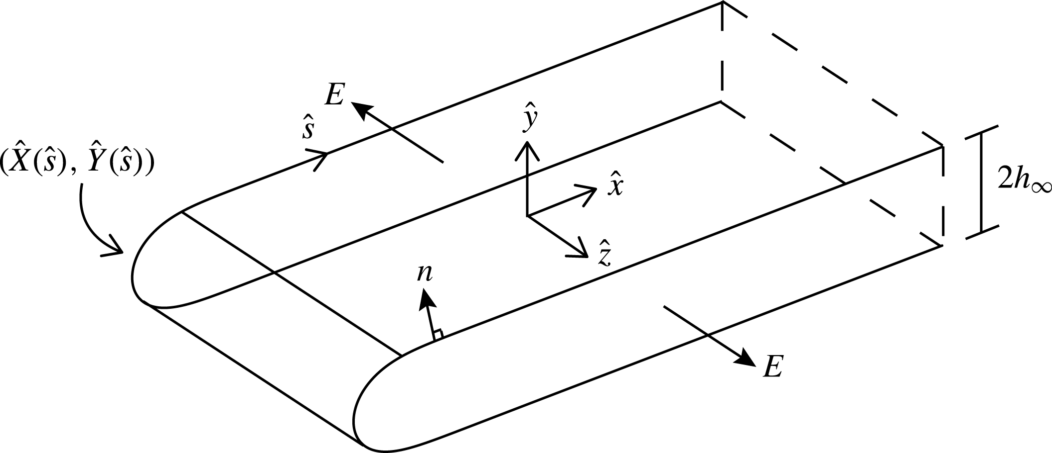
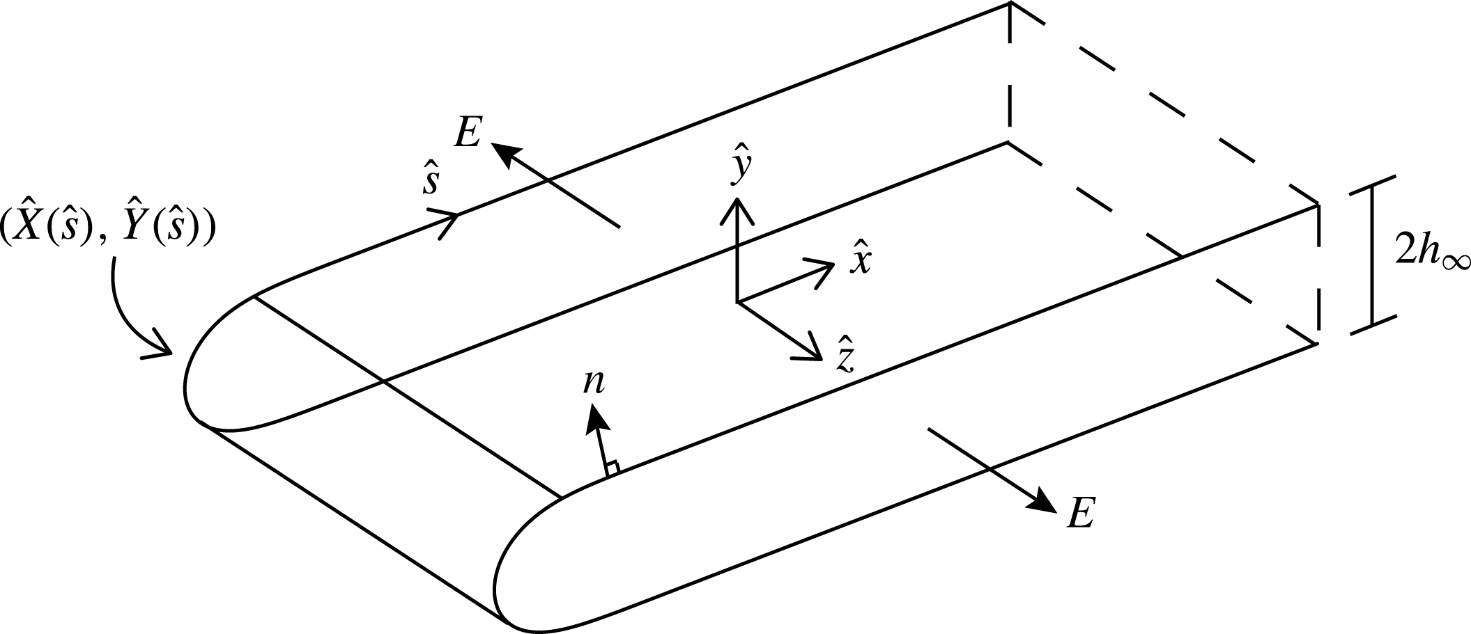
We consider the motion of the edge of a semi-infinite planar fluid sheet with constant cross-section, which is being stretched in the direction parallel to the edge, as in figure 1. We take the fluid parameters
 $\unicode[STIX]{x1D707}$
and
 $\unicode[STIX]{x1D6FE}$
and the strain rate
 $E$
along the edge all to be uniform, but we allow the strain rate to vary with time
 $\hat{t}$
. We consider a sheet with uniform thickness
 $2h_{\infty }(\hat{t})$
in the far field.
We define a coordinate system
 $(\hat{x},{\hat{y}},\hat{z})$
oriented as shown in figure 1, with the
 $\hat{z}$
axis parallel to the edge. The
 $(\hat{x},{\hat{y}})$
-plane is normal to the edge, with the mid-plane of the sheet lying in the
 $(\hat{x},\hat{z})$
-plane. The corresponding three-dimensional velocity
 $\hat{\boldsymbol{u}}=(\hat{u} ,\hat{v},{\hat{w}})$
satisfies the Stokes equations
 $$\begin{eqnarray}\displaystyle & \displaystyle \hat{\unicode[STIX]{x1D735}}\boldsymbol{\cdot }\hat{\boldsymbol{u}}=0,\quad -\hat{\unicode[STIX]{x1D735}}\hat{p}+\unicode[STIX]{x1D707}\hat{\unicode[STIX]{x1D6FB}}^{2}\hat{\boldsymbol{u}}=\mathbf{0}. & \displaystyle\end{eqnarray}$$
Since the stretching is uniform, we can choose the origin of
 $\hat{z}$
such that
 ${\hat{w}}=E(\hat{t})\hat{z}$
, where
 $E(\hat{t})$
is the strain rate. We parametrise the surface shape by the arclength
 ${\hat{s}}$
and time
 $\hat{t}$
as
 $\hat{\boldsymbol{X}}=(\hat{X}({\hat{s}},\hat{t}),{\hat{Y}}({\hat{s}},\hat{t}))$
, so that
 ${\hat{Y}}\rightarrow h_{\infty }$
as
 ${\hat{s}}\rightarrow \infty$
.
Sketch of the sheet, with the
 $\hat{z}$
-axis parallel to the edge. The far-field thickness
 $2h_{\infty }$
, the longitudinal strain rate
 $E$
and the fluid parameters
 $\unicode[STIX]{x1D707}$
and
 $\unicode[STIX]{x1D6FE}$
are uniform.
Since
 $\hat{u}$
,
 $\hat{v}$
,
 $\hat{p}$
and
 $E$
are independent of
 $\hat{z}$
, the local mass-conservation equation and the momentum equation for the two-dimensional in-section velocity
 $\hat{\boldsymbol{u}}_{H}=(\hat{u} ,\hat{v})$
reduce to
 $$\begin{eqnarray}\displaystyle & \displaystyle \hat{\unicode[STIX]{x1D735}}\boldsymbol{\cdot }\hat{\boldsymbol{u}}_{H}=-E,\quad -\hat{\unicode[STIX]{x1D735}}\hat{p}+\unicode[STIX]{x1D707}\hat{\unicode[STIX]{x1D6FB}}^{2}\boldsymbol{u}_{H}=\mathbf{0}, & \displaystyle\end{eqnarray}$$
with kinematic and dynamic boundary conditions on the surface
 $$\begin{eqnarray}\displaystyle & \displaystyle {\displaystyle \frac{\unicode[STIX]{x2202}\hat{\boldsymbol{X}}}{\unicode[STIX]{x2202}\hat{t}}}\boldsymbol{\cdot }\boldsymbol{n}=\hat{\boldsymbol{u}}_{H}\boldsymbol{\cdot }\boldsymbol{n},\quad \text{and}\quad -\hat{p}\boldsymbol{n}+\unicode[STIX]{x1D707}(\hat{\unicode[STIX]{x1D735}}\hat{\boldsymbol{u}}_{H}+(\hat{\unicode[STIX]{x1D735}}\hat{\boldsymbol{u}}_{H})^{\text{T}})\boldsymbol{\cdot }\boldsymbol{n}=-\unicode[STIX]{x1D6FE}\hat{\unicode[STIX]{x1D705}}\boldsymbol{n}, & \displaystyle\end{eqnarray}$$
where
 $\hat{\unicode[STIX]{x1D705}}=\hat{\unicode[STIX]{x1D735}}\boldsymbol{\cdot }\boldsymbol{n}$
is the curvature of the surface and
 $\boldsymbol{n}$
the surface normal.
Consider the stress
 $\hat{\unicode[STIX]{x1D748}}=-\hat{p}\unicode[STIX]{x1D644}+\unicode[STIX]{x1D707}(\hat{\unicode[STIX]{x1D735}}\hat{\boldsymbol{u}}_{H}+(\hat{\unicode[STIX]{x1D735}}\hat{\boldsymbol{u}}_{H})^{\text{T}})$
in the far field. The sheet is almost flat and uniform so, by translational symmetry, the far-field stress is independent of
 $\hat{x}$
at leading order. In the far field, we have
 ${\hat{Y}}\sim h_{\infty }$
, so
 $\boldsymbol{n}\sim (0,1)$
and the curvature is negligible. Hence the stress boundary condition (2.3b
) gives
 $\hat{\unicode[STIX]{x1D70E}}_{xy}=0$
and
 $\hat{\unicode[STIX]{x1D70E}}_{yy}=0$
in the far field. In addition, the viscous force over the sheet in the far field,
 $2h_{\infty }\unicode[STIX]{x1D70E}_{xx}$
, must balance the net force from surface tension,
 $2\unicode[STIX]{x1D6FE}$
. Together, these conditions specify
 $\hat{\unicode[STIX]{x1D748}}$
in the far field, and then local mass conservation (2.2) gives the far-field velocity and pressure as
 $$\begin{eqnarray}\displaystyle & \displaystyle \hat{\boldsymbol{u}}_{H}\sim {\displaystyle \frac{\unicode[STIX]{x1D6FE}}{4\unicode[STIX]{x1D707}h_{\infty }}}(-\hat{x},{\hat{y}})-{\displaystyle \frac{E}{2}}(\hat{x},{\hat{y}}),\quad \hat{p}\sim {\displaystyle \frac{\unicode[STIX]{x1D6FE}}{2h_{\infty }}}-\unicode[STIX]{x1D707}E\quad \text{as }\hat{x}\rightarrow \infty . & \displaystyle\end{eqnarray}$$
Here, we have chosen the origin so that the velocity grows linearly in the far field, without a constant term. Since the Stokes equations are linear, we may add any solid-body motion to our solution below.
The kinematic boundary condition (2.3a ) with the far-field velocity (2.4) gives
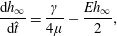 $$\begin{eqnarray}\displaystyle & \displaystyle {\displaystyle \frac{\text{d}h_{\infty }}{\text{d}\hat{t}}}={\displaystyle \frac{\unicode[STIX]{x1D6FE}}{4\unicode[STIX]{x1D707}}}-{\displaystyle \frac{Eh_{\infty }}{2}}, & \displaystyle\end{eqnarray}$$
and so we have found the effect of the stretching and capillarity on the far-field thickness.
Note that the two-dimensional velocity
 $\boldsymbol{u}_{H}$
does not satisfy the two-dimensional Stokes equations when
 $E\neq 0$
because
 $\unicode[STIX]{x1D735}\boldsymbol{\cdot }\boldsymbol{u}_{H}=-E$
and so mass is not conserved. However, if subtract the far-field velocity and non-dimensionalise by setting
 $$\begin{eqnarray}\displaystyle & \displaystyle {\displaystyle \frac{\unicode[STIX]{x1D6FE}}{\unicode[STIX]{x1D707}}}(u,v)=(\hat{u} ,\hat{v})-{\displaystyle \frac{\unicode[STIX]{x1D6FE}}{4\unicode[STIX]{x1D707}h_{\infty }}}(-\hat{x},{\hat{y}})+{\displaystyle \frac{E}{2}}(\hat{x},{\hat{y}}), & \displaystyle\end{eqnarray}$$
then
 $\boldsymbol{u}=(u,v)$
satisfies the Stokes equations. We also subtract the far-field pressure, and non-dimensionalise lengths with respect to
 $h_{\infty }$
by setting
 $$\begin{eqnarray}\displaystyle & \displaystyle p={\displaystyle \frac{h_{\infty }}{\unicode[STIX]{x1D6FE}}}\hat{p}-{\displaystyle \frac{1}{2}}+Ca,\quad \boldsymbol{x}={\displaystyle \frac{\hat{\boldsymbol{x}}}{h_{\infty }}},\quad \boldsymbol{X}={\displaystyle \frac{\hat{\boldsymbol{X}}}{h_{\infty }}}\quad \text{and}\quad \unicode[STIX]{x1D705}=h_{\infty }\hat{\unicode[STIX]{x1D705}}, & \displaystyle\end{eqnarray}$$
where
 $Ca=\unicode[STIX]{x1D707}Eh_{\infty }/\unicode[STIX]{x1D6FE}$
is the capillary number. Then the two-dimensional Stokes equations (2.2) become
 $$\begin{eqnarray}\displaystyle & \displaystyle -\unicode[STIX]{x1D735}p+\unicode[STIX]{x1D6FB}^{2}\boldsymbol{u}=\mathbf{0},\quad \unicode[STIX]{x1D735}\boldsymbol{\cdot }\boldsymbol{u}=0, & \displaystyle\end{eqnarray}$$
where the derivatives are taken with respect to the scaled variables. The stress boundary condition (2.3b ) on the surface becomes
 $$\begin{eqnarray}\displaystyle & \displaystyle -p\boldsymbol{n}+(\unicode[STIX]{x1D735}\boldsymbol{u}+\unicode[STIX]{x1D735}\boldsymbol{u}^{\text{T}})\boldsymbol{\cdot }\boldsymbol{n}=-\unicode[STIX]{x1D705}\boldsymbol{n}+\left(\begin{array}{@{}cc@{}}1 & 0\\ 0 & 0\end{array}\right)\boldsymbol{\cdot }\boldsymbol{n}, & \displaystyle\end{eqnarray}$$
and in the far field
 $$\begin{eqnarray}\displaystyle & \displaystyle X\rightarrow \infty ,\quad Y\rightarrow \pm 1,\quad \boldsymbol{u}\rightarrow \mathbf{0}\quad \text{as }s\rightarrow \pm \infty . & \displaystyle\end{eqnarray}$$
We note that, by subtracting the far-field velocity in the definition of
 $\boldsymbol{u}$
, we have removed
 $E$
from the Stokes problem entirely at any given time. Moreover, if we rescale the time variable appropriately, then the kinematic boundary condition (2.3a
) becomes
 $$\begin{eqnarray}\displaystyle & \displaystyle {\displaystyle \frac{\unicode[STIX]{x2202}\boldsymbol{X}}{\unicode[STIX]{x2202}t}}\boldsymbol{\cdot }\boldsymbol{n}=\boldsymbol{u}\boldsymbol{\cdot }\boldsymbol{n}-{\displaystyle \frac{1}{2}}(x,0)\boldsymbol{\cdot }\boldsymbol{n},\quad \text{where}~{\displaystyle \frac{\text{d}t}{\text{d}\hat{t}}}={\displaystyle \frac{\unicode[STIX]{x1D6FE}}{\unicode[STIX]{x1D707}h_{\infty }(\hat{t})}} & \displaystyle\end{eqnarray}$$
and
 $h_{\infty }(\hat{t})$
is given by the solution to (2.5). We have therefore removed the time-dependent stretching from the problem entirely, and rather than solving a family of problems parametrised by
 $Ca$
, we need only solve a single Stokes problem (2.8)–(2.11). Independent of the initial conditions, we expect that the solution of (2.8)–(2.11) will tend to a steady state,
 $\boldsymbol{n}\boldsymbol{\cdot }\unicode[STIX]{x2202}\boldsymbol{X}/\unicode[STIX]{x2202}t=0$
, in these scaled variables, which corresponds to a similarity solution with length scale
 $h_{\infty }(\hat{t})$
in the original variables. We solve for this similarity solution numerically below.
3 Numerical solution
We divide the sheet into two regions: a local region
 $S_{1}=\{(X,Y):X-X(0,t)\leqslant 4\}$
and a far-field region
 $S_{2}=\{(X,Y):X-X(0,t)>4\}$
. In
 $S_{1}$
, we solve for the velocity
 $\boldsymbol{u}$
with the boundary integral equation for Stokes flow (e.g. Pozrikidis Reference Pozrikidis1992). For a point
 $\boldsymbol{y}$
on the surface,
 $$\begin{eqnarray}\displaystyle & \displaystyle \int _{S}\unicode[STIX]{x1D645}(\boldsymbol{y}-\boldsymbol{x})\boldsymbol{\cdot }\unicode[STIX]{x1D748}\boldsymbol{\cdot }\boldsymbol{n}\,\text{d}s_{\boldsymbol{x}}+\int _{S}\boldsymbol{u}\boldsymbol{\cdot }\unicode[STIX]{x1D646}(\boldsymbol{y}-\boldsymbol{x})\boldsymbol{\cdot }\boldsymbol{n}\,\text{d}s_{\boldsymbol{x}}={\textstyle \frac{1}{2}}\boldsymbol{u}(\boldsymbol{y}), & \displaystyle\end{eqnarray}$$
where
 $$\begin{eqnarray}\displaystyle & \displaystyle \unicode[STIX]{x1D645}(\boldsymbol{x})={\displaystyle \frac{1}{4\unicode[STIX]{x03C0}}}\left(-\unicode[STIX]{x1D644}\log |\boldsymbol{x}|+{\displaystyle \frac{\boldsymbol{x}\boldsymbol{x}}{|\boldsymbol{x}|^{2}}}\right),\quad \unicode[STIX]{x1D646}(\boldsymbol{x})=-{\displaystyle \frac{\boldsymbol{x}\boldsymbol{x}\boldsymbol{x}}{\unicode[STIX]{x03C0}|\boldsymbol{x}|^{4}}}, & \displaystyle\end{eqnarray}$$
and
 $\unicode[STIX]{x1D748}\boldsymbol{\cdot }\boldsymbol{n}$
is given by (2.9). We discretise the surface in
 $S_{1}$
with grid points at
 $(X(s_{i}),Y(s_{i}))$
for
 $1\leqslant i\leqslant n$
. Between the grid points, we interpolate
 $X(s)$
and
 $Y(s)$
with quintic splines. In appendix A, we derive an asymptotic series for the far-field decay of the shape, which we use here to set
 $Y^{\prime }(s_{n})$
and
 $Y^{\prime \prime }(s_{n})$
as boundary conditions on the spline. We also use the asymptotic form of
 $\boldsymbol{u}$
to integrate (3.1) numerically for
 $\boldsymbol{x}$
in
 $S_{2}$
.
For any
 $\boldsymbol{y}$
on the surface, the first integrand in (3.1) diverges at
 $s_{\boldsymbol{x}}=s_{\boldsymbol{y}}$
, where
 $\unicode[STIX]{x1D645}(\boldsymbol{y}-\boldsymbol{x})\boldsymbol{\cdot }\unicode[STIX]{x1D748}\boldsymbol{\cdot }\boldsymbol{n}\sim \log |s_{\boldsymbol{y}}-s_{\boldsymbol{x}}|\,\unicode[STIX]{x1D748}(\boldsymbol{y})\boldsymbol{\cdot }\boldsymbol{n}$
. We subtract
 $\log |s_{\boldsymbol{y}}-s_{\boldsymbol{x}}|\,\unicode[STIX]{x1D748}(\boldsymbol{y})\boldsymbol{\cdot }\boldsymbol{n}$
from the integrand on panels where the integrand diverges and integrate the remainder with seven-point Gaussian quadrature. The subtracted term can be integrated analytically.
The second integral in (3.1) depends on the unknown velocity
 $\boldsymbol{u}$
. We discretise this integral by considering a set of test functions for the velocity. For each component of the velocity at each grid point in
 $S_{1}$
, we set a test function to 1 at that point and 0 on the other points. We interpolate the velocity with quintic splines and again use Gaussian integration to find the contribution to the integral. The result of this discretisation is a matrix problem for the velocity components in
 $S_{1}$
, which we invert for the velocity.
We advect the surface with the kinematic boundary condition (2.11), using a time step of order
 $10^{-2}$
. After each advection step, we rescale the shape so that
 $Y(s_{n})-1$
matches the asymptotic expression derived in appendix A. We repeat and step forward in time up to
 $t=30$
to allow any transients to decay.
We initialised the shape with a rectangle of fluid rounded by a semicircular cap. With 51 points spaced so that
 $\unicode[STIX]{x0394}s\approx 0.1$
, the far end of the rectangle is initially at
 $X(s_{n})\approx 4.4$
.
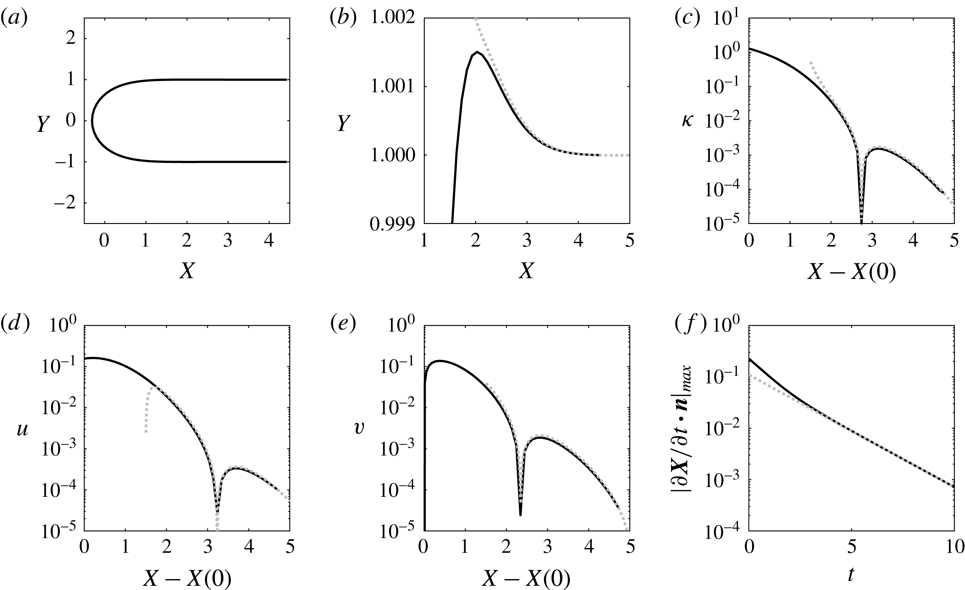
The shape relaxes to the steady-state solution shown in figure 2(a). The edge of the sheet is at
 $X(0)=-0.312$
, and we recall that the origin of
 $X$
(the frame of reference) was chosen such that the far-field velocity is given by (2.4). This choice implies that the steady-state shape must have the same area as a rectangle of height 2 with its end at
 $X=0$
. The sheet thickness does not monotonically decay to the far-field thickness; the maximum half-thickness is
 $Y=1+1.5\times 10^{-3}$
at
 $X=2.03$
, as shown in figure 2(b). Changing the number of points used to discretise the surface does not affect these constants, so we can be confident that we have resolved the shape accurately.
The numerically calculated steady-state solution to (2.8)–(2.11) (solid lines) and its far-field behaviour (dashed lines). (a) The self-similar shape of the retracting edge. (b) The decay of the shape to its far-field thickness
 $Y=1$
. (c) The full curvature
 $\unicode[STIX]{x1D705}$
of the surface. (d,e) The velocity components
 $\boldsymbol{u}=(u,v)$
, defined by (2.6). (f) The maximum of the normal velocity at each time step. In (b–e), the asymptotic solution found in appendix A is shown for comparison.
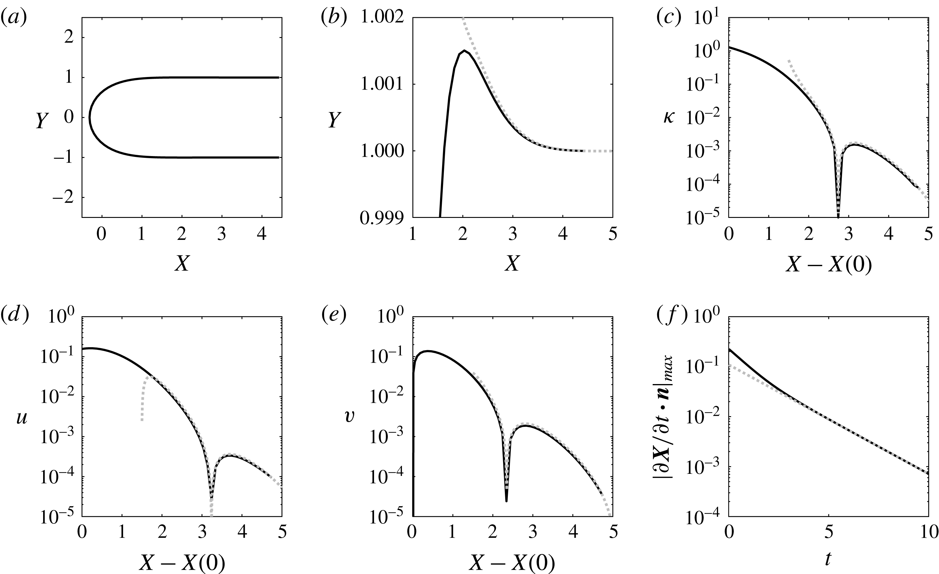
We can compare the shape and velocity with the far-field asymptotic series given in appendix A, calculating the amplitude
 $A_{1,0}$
of the series from the final velocity components
 $(u(s_{n}),v(s_{n}))$
. Figure 2(b) shows the asymptotic decay of the surface shape to its far-field thickness, and there is good agreement between the numerically calculated similarity solution and the asymptotic series. The full curvature is compared with
 $Y_{XX}$
in figure 2(c), showing that the approximation
 $\unicode[STIX]{x1D705}\sim Y_{XX}$
holds far from the edge. The velocity components are shown in figure 2(d,e). The numerically calculated values agree well with the far-field asymptotic series not only at
 $s_{n}$
, where the series is set to match the velocity components, but also in some overlap region where
 $X-X(0)\gtrsim 2$
. This verifies the accuracy of the solution.
The similarity solution is stable; changing the initial shape of the sheet does not affect the resultant steady state. Moreover, our numerical solution shows the decay rate of the slowest-decaying mode. Figure 2(f) shows the maximum absolute value of the normal component of the velocity at each time step. After some shorter-lived transients, the residual normal velocity decays exponentially with time. We fit an exponential to the data between
 $t=5$
and
 $t=10$
and find that the slowest mode decays proportional to
 $\text{e}^{-0.50t}$
(shown as a dashed line in figure 2
f). We can therefore be sure that the solution has converged to the required accuracy by time
 $t=30$
.
4 Discussion
We have solved for the free-surface motion of a sheet of viscous fluid surrounded by air, driven by surface tension on the interface and by uniform stretching along the edge. The solution is universal, giving the retraction of a viscous sheet at any capillary number. With the choice of variables given above (in (2.6), (2.7) and (2.11)), there is a steady-state similarity solution for the retraction of the edge.
The shape of the similarity solution shows that surface tension invariably causes a minor thickening of the edge by a maximum of just 0.15 %, a perturbation which decays exponentially with distance on the scale of the sheet thickness. This thickening is distinct from the effects of inertia or non-uniform stretching in the bulk of the sheet, which can cause the sheet to thicken on a much longer length scale (Brenner & Gueyffier Reference Brenner and Gueyffier1999; O’Kiely et al. Reference O’Kiely, Breward, Griffiths, Howell and Lange2015).
The exponential decay of the near-edge solution to the far-field linear flow justifies the use of a resultant stress condition in long-wavelength models for fluid sheets. As an example, we consider the application to bubble coalescence. In our previous work (Munro et al.
Reference Munro, Anthony, Basaran and Lister2015), we considered the thin-sheet flow around the growing hole that joins two coalescing bubbles. In that paper, we used a resultant stress condition at the edge of the thin sheet to model the stress from surface tension on the sheet. We found the thickness of the sheet at the edge to be
 $2\unicode[STIX]{x1D6FE}\hat{t}/5\unicode[STIX]{x1D707}$
by analysis of the boundary conditions at the edge. We can now resolve the tightly curved shape of the surface. The hole grows as
 $\hat{t}^{1/2}$
, and the azimuthal strain rate is therefore
 $E=1/(2\hat{t})$
. With this strain rate, we can solve the differential equation (2.5) for
 $h_{\infty }=\unicode[STIX]{x1D6FE}\hat{t}/5\unicode[STIX]{x1D707}$
in agreement with our previous result. The similarity solution above gives the shape of the curved edge. Relative to the edge position in the thin-sheet model, the edge of the curved sheet is therefore at
 $\hat{x}=-0.0625\unicode[STIX]{x1D6FE}\hat{t}/\unicode[STIX]{x1D707}$
, which is an asymptotically small correction to the
 $\hat{t}^{1/2}$
growth at early times.
The solution above neglects inertia. Our typical time scale and length scale are
 $T\propto \unicode[STIX]{x1D707}h_{\infty }/\unicode[STIX]{x1D6FE}$
and
 $L\propto h_{\infty }$
, which we can use to compare terms in the Navier–Stokes equations. The inertial terms are smaller than the viscous terms if
 $\unicode[STIX]{x1D70C}/T\ll \unicode[STIX]{x1D707}/L^{2}$
, which is the case if
 $Oh^{2}\gg 1$
, where
 $Oh=\unicode[STIX]{x1D707}/\sqrt{\unicode[STIX]{x1D70C}h_{\infty }\unicode[STIX]{x1D6FE}}$
is the Ohnesorge number based on the sheet thickness. If the sheet is sufficiently thin or viscous that
 $Oh^{2}\gg 1$
, then the solution above will apply. Note that in the bulk of the sheet, the typical length scale will be larger and inertia may enter the long-wavelength equations (e.g. Brenner & Gueyffier Reference Brenner and Gueyffier1999; Savva & Bush Reference Savva and Bush2009; Munro et al.
Reference Munro, Anthony, Basaran and Lister2015).
We have taken the strain rate
 $E$
and the fluid parameters
 $\unicode[STIX]{x1D707}$
and
 $\unicode[STIX]{x1D6FE}$
to be independent of
 $\hat{z}$
. If
 $E$
slowly varies along the sheet edge, for example in a sheet falling under its own weight, then we could replace the time derivatives in the kinematic boundary condition with material derivatives, and follow a fluid parcel down the sheet as the local stretching rate changes. If the fluid parameters change slowly along the sheet edge, for example in a cooling glass sheet, then we could also adapt the rescaled time variable (2.11) with the time-dependent fluid parameters experienced by a fluid parcel, which would again give the problem solved above. In any case, the shape approaches the similarity solution given above.
Acknowledgements
J.P.M. gratefully acknowledges an Engineering and Physical Sciences Research Council studentship. All data accompanying this publication are directly available within the publication.
Appendix A. Far-field steady-state asymptotic behaviour
We solve for the far-field Stokes flow, driven by surface tension on the free surface. We seek the asymptotic form of the similarity solution.
Previous work on Stokes flows in a rectangular geometry with rigid walls expands the streamfunction in a series of eigenfunctions (e.g. Fadle Reference Fadle1940; Papkovich Reference Papkovich1940; Moffatt Reference Moffatt1964). Here, the flow must instead satisfy free-surface boundary conditions, with forcing from surface tension.
We use a streamfunction
 $\unicode[STIX]{x1D713}$
with
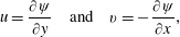 $$\begin{eqnarray}\displaystyle & \displaystyle u={\displaystyle \frac{\unicode[STIX]{x2202}\unicode[STIX]{x1D713}}{\unicode[STIX]{x2202}y}}\quad \text{and}\quad v=-{\displaystyle \frac{\unicode[STIX]{x2202}\unicode[STIX]{x1D713}}{\unicode[STIX]{x2202}x}}, & \displaystyle\end{eqnarray}$$
where
 $\unicode[STIX]{x1D713}$
satisfies the biharmonic equation
 $\unicode[STIX]{x1D6FB}^{4}\unicode[STIX]{x1D713}=0$
. On the surface
 $Y(x)\approx 1$
, the normal is
 $\boldsymbol{n}\sim (-Y_{x},1)$
since
 $|Y_{x}|\ll 1$
by (2.10). Using
 $|\unicode[STIX]{x1D713}|\ll 1$
also, the kinematic boundary condition (2.11) can be linearised to
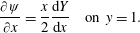 $$\begin{eqnarray}\displaystyle & \displaystyle {\displaystyle \frac{\unicode[STIX]{x2202}\unicode[STIX]{x1D713}}{\unicode[STIX]{x2202}x}}={\displaystyle \frac{x}{2}}{\displaystyle \frac{\text{d}Y}{\text{d}x}}\quad \text{on }y=1. & \displaystyle\end{eqnarray}$$
Similarly, the stress boundary conditions (2.9) become
 $$\begin{eqnarray}\displaystyle & \displaystyle -p-2{\displaystyle \frac{\unicode[STIX]{x2202}^{2}\unicode[STIX]{x1D713}}{\unicode[STIX]{x2202}x\unicode[STIX]{x2202}y}}={\displaystyle \frac{\text{d}^{2}Y}{\text{d}x^{2}}}\quad \text{and}\quad {\displaystyle \frac{\unicode[STIX]{x2202}^{2}\unicode[STIX]{x1D713}}{\unicode[STIX]{x2202}x^{2}}}-{\displaystyle \frac{\unicode[STIX]{x2202}^{2}\unicode[STIX]{x1D713}}{\unicode[STIX]{x2202}y^{2}}}={\displaystyle \frac{\text{d}Y}{\text{d}x}}\quad \text{on }y=1. & \displaystyle\end{eqnarray}$$
We take an
 $x$
-derivative of (A 3a
) and use the Stokes equations (2.8) to eliminate
 $p$
in favour of
 $\unicode[STIX]{x1D713}$
. Then we can eliminate
 $Y$
with the kinematic boundary condition, giving boundary conditions on
 $y=1$
in terms of
 $\unicode[STIX]{x1D713}$
alone:
 $$\begin{eqnarray}\displaystyle & \displaystyle -{\displaystyle \frac{\unicode[STIX]{x2202}^{3}\unicode[STIX]{x1D713}}{\unicode[STIX]{x2202}y^{3}}}-3{\displaystyle \frac{\unicode[STIX]{x2202}^{3}\unicode[STIX]{x1D713}}{\unicode[STIX]{x2202}x^{2}\unicode[STIX]{x2202}y}}=2{\displaystyle \frac{\unicode[STIX]{x2202}^{2}}{\unicode[STIX]{x2202}x^{2}}}\left({\displaystyle \frac{1}{x}}{\displaystyle \frac{\unicode[STIX]{x2202}\unicode[STIX]{x1D713}}{\unicode[STIX]{x2202}x}}\right)\quad \text{and}\quad {\displaystyle \frac{\unicode[STIX]{x2202}^{2}\unicode[STIX]{x1D713}}{\unicode[STIX]{x2202}x^{2}}}-{\displaystyle \frac{\unicode[STIX]{x2202}^{2}\unicode[STIX]{x1D713}}{\unicode[STIX]{x2202}y^{2}}}={\displaystyle \frac{2}{x}}{\displaystyle \frac{\unicode[STIX]{x2202}\unicode[STIX]{x1D713}}{\unicode[STIX]{x2202}x}}\quad \text{on }y=1. & \displaystyle \nonumber\\ \displaystyle & & \displaystyle\end{eqnarray}$$
If
 $Y$
were constant, then the surface would be flat and completely stress-free, and we would expect exponentially decaying eigensolutions to the biharmonic equation. However, such eigensolutions have a non-zero normal velocity on
 $y=1$
, which by (A 2) deflects the interface away from uniformity, which then, by (A 3), produces stresses that drive further flow. Consideration of the form of the boundary conditions suggests that each eigenmode drives a series of algebraically smaller corrections, and so we seek a solution of the form
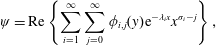 $$\begin{eqnarray}\displaystyle & \displaystyle \unicode[STIX]{x1D713}=\text{Re}\left\{\mathop{\sum }_{i=1}^{\infty }\mathop{\sum }_{j=0}^{\infty }\unicode[STIX]{x1D719}_{i,j}(y)\text{e}^{-\unicode[STIX]{x1D706}_{i}x}x^{\unicode[STIX]{x1D70E}_{i}-j}\right\}, & \displaystyle\end{eqnarray}$$
where the
 $\unicode[STIX]{x1D706}_{i}$
are complex eigenvalues of the free-surface problem, the functions
 $\unicode[STIX]{x1D719}_{i,j}(y)$
are the eigenfunctions and the terms
 $j\geqslant 1$
are the corrections. By symmetry, the functions
 $\unicode[STIX]{x1D719}_{i,j}(y)$
are odd. The offset constants
 $\unicode[STIX]{x1D70E}_{i}$
in the exponents are shown below to be necessary as the forcing of the correction is resonant, with the same spatial structure as the eigensolutions of the free-surface problem.
We consider the leading-order term,
 $j=0$
, for the
 $i$
th mode, and find the biharmonic equation at leading order in
 $x$
gives the odd solution
 $$\begin{eqnarray}\displaystyle & \displaystyle \unicode[STIX]{x1D719}_{i,0}(y)=A_{i,0}y\cos \unicode[STIX]{x1D706}_{i}y+B_{i,0}\sin \unicode[STIX]{x1D706}_{i}y & \displaystyle\end{eqnarray}$$
for some constants
 $A_{i,0}$
and
 $B_{i,0}$
. The boundary conditions (A 4) yield, at leading order in
 $x$
,
 $$\begin{eqnarray}\displaystyle & \displaystyle \unicode[STIX]{x1D647}_{i}\left(\begin{array}{@{}c@{}}A_{i,0}\\ B_{i,0}\end{array}\right)=\mathbf{0},\quad \text{where}~\unicode[STIX]{x1D647}_{i}=\left(\begin{array}{@{}cc@{}}\sin \unicode[STIX]{x1D706}_{i} & -\text{cos}\,\unicode[STIX]{x1D706}_{i}\\ \sin \unicode[STIX]{x1D706}_{i}+\unicode[STIX]{x1D706}_{i}\cos \unicode[STIX]{x1D706}_{i} & \unicode[STIX]{x1D706}_{i}\sin \unicode[STIX]{x1D706}_{i}\end{array}\right). & \displaystyle\end{eqnarray}$$
This is an eigenvalue problem for
 $\unicode[STIX]{x1D706}_{i}$
. There are non-trivial solutions only if
 $\det \unicode[STIX]{x1D647}_{i}=0$
, which requires
 $$\begin{eqnarray}\displaystyle & \displaystyle \sin 2\unicode[STIX]{x1D706}_{i}+2\unicode[STIX]{x1D706}_{i}=0. & \displaystyle\end{eqnarray}$$
We number the roots of (A 8) in order of increasing real part, with
 $\unicode[STIX]{x1D706}_{1}\approx 2.106+1.125\text{i}$
,
 $\unicode[STIX]{x1D706}_{2}\approx 5.356+1.552\text{i}$
and so on. With these eigenvalues,
 $$\begin{eqnarray}\displaystyle & \displaystyle \unicode[STIX]{x1D719}_{i,0}(y)=A_{i,0}(y\cos \unicode[STIX]{x1D706}_{i}y+\tan \unicode[STIX]{x1D706}_{i}\sin \unicode[STIX]{x1D706}_{i}y). & \displaystyle\end{eqnarray}$$
We note that, while the eigenvalues are the same as for the rigid boundary condition (Moffatt Reference Moffatt1964), these stress-free eigenfunctions are not.
At the next algebraic order,
 $j=1$
, and the biharmonic equation gives
 $$\begin{eqnarray}\displaystyle & \displaystyle \unicode[STIX]{x1D719}_{i,1}(y)=A_{i,0}\unicode[STIX]{x1D70E}_{i}y^{2}\sin \unicode[STIX]{x1D706}_{i}y+A_{i,1}y\cos \unicode[STIX]{x1D706}_{i}y+B_{i,1}\sin \unicode[STIX]{x1D706}_{i}y. & \displaystyle\end{eqnarray}$$
The first term is driven by the leading-order flow through the Stokes equations and the other terms are the complementary solutions of the biharmonic equation. The boundary conditions at this order become
 $$\begin{eqnarray}\displaystyle & \displaystyle \unicode[STIX]{x1D647}_{i}\left(\begin{array}{@{}c@{}}A_{i,1}\\ B_{i,1}\end{array}\right)=A_{i,0}\left(\begin{array}{@{}c@{}}\unicode[STIX]{x1D70E}_{i}\cos \unicode[STIX]{x1D706}_{i}-\sec \unicode[STIX]{x1D706}_{i}\\ \unicode[STIX]{x1D70E}_{i}(2\cos \unicode[STIX]{x1D706}_{i}-\unicode[STIX]{x1D706}_{i}\sin \unicode[STIX]{x1D706}_{i})-\sec \unicode[STIX]{x1D706}_{i}\end{array}\right), & \displaystyle\end{eqnarray}$$
which is a singular matrix problem for
 $A_{i,1}$
and
 $B_{i,1}$
. The right-hand side lies in the image of
 $\unicode[STIX]{x1D647}_{i}$
only if
 $\unicode[STIX]{x1D70E}_{i}=1/2$
. With this condition, we have
 $$\begin{eqnarray}\displaystyle & \displaystyle \unicode[STIX]{x1D719}_{i,1}=A_{i,0}\left({\textstyle \frac{1}{2}}(1+y^{2})+\tan ^{2}\unicode[STIX]{x1D706}_{i}\right)\sin \unicode[STIX]{x1D706}y+A_{i,1}(y\cos \unicode[STIX]{x1D706}_{i}y+\tan \unicode[STIX]{x1D706}_{i}\sin \unicode[STIX]{x1D706}_{i}y). & \displaystyle\end{eqnarray}$$
This solution includes a multiple of the stress-free eigensolution, the magnitude
 $A_{i,1}$
of which will be set at the next algebraic order.
We now proceed through algebraic orders by induction. For
 $j\geqslant 2$
, suppose that we know
 $B_{i,k}$
in terms of
 $A_{i,0}$
for all
 $k<j$
and that we know
 $A_{i,k}$
in terms of
 $A_{i,0}$
for all
 $k<j-1$
. Then the boundary conditions at the
 $j$
th order give
 $$\begin{eqnarray}\displaystyle & \displaystyle \unicode[STIX]{x1D647}_{i}(A_{i,j},B_{i,j})=A_{i,0}\boldsymbol{e}_{1}+A_{i,j-1}\boldsymbol{e}_{2}, & \displaystyle\end{eqnarray}$$
where
 $\boldsymbol{e}_{1}$
and
 $\boldsymbol{e}_{2}$
are vectors depending on
 $\unicode[STIX]{x1D706}_{i}$
. There is a solution only if the right-hand side lies in the image of
 $\unicode[STIX]{x1D647}_{i}$
, and this requirement gives an expression for
 $A_{i,j-1}$
in terms of
 $A_{i,0}$
. The corresponding solution to the matrix problem (A 13) gives
 $B_{i,j}$
. We can therefore induct to arbitrary algebraic order for each
 $\unicode[STIX]{x1D706}_{i}$
.
For the numerical solution above, we used the first ten algebraic terms corresponding to the first eigenvalue with
 $i=1$
, and we neglected the terms corresponding to further eigenvalues
 $i>1$
as they are asymptotically smaller. For this truncated series, the velocity and shape are proportional to
 $A_{1,0}$
. At each time step, we set the series for the velocity at
 $s_{n}$
equal to the numerically calculated
 $\boldsymbol{u}(s_{n})$
from the previous time step, and we solved for
 $A_{1,0}$
. We used this in our boundary condition for
 $Y$
; we interpolated
 $Y(s)$
with a quintic spline, with
 $Y^{\prime }(s_{n})$
and
 $Y^{\prime \prime }(s_{n})$
given by the truncated asymptotic series.
As the transients decayed, the constant
 $A_{1,0}$
converged. For the steady-state solution, we found the numerical value
 $A_{1,0}=0.05$
. This gives the series solution shown with dashed lines in figure 2.
The accuracy of the numerical solution depends on the size of the neglected terms. We have truncated the shape at
 $x\approx 4$
, so the further exponential terms are smaller by a factor of approximately
 $|\text{e}^{4(\unicode[STIX]{x1D706}_{1}-\unicode[STIX]{x1D706}_{2})}|\approx 2\times 10^{-6}$
. In addition, the further algebraic terms are smaller than the leading order by a factor of approximately
 $4^{-10}\approx 1\times 10^{-6}$
. In forming this linearised problem, we have neglected quadratic terms that are smaller by a factor of approximately
 $|\text{e}^{-4\unicode[STIX]{x1D706}_{1}}|\approx 2\times 10^{-4}$
. This gives an estimate of the accuracy of the solution.
The leading-order expressions for the displacement and the velocity on the surface are the real parts of
 $$\begin{eqnarray}\displaystyle & \displaystyle (u,v)\sim A_{1,0}\text{e}^{-\unicode[STIX]{x1D706}_{1}x}x^{1/2}(\cos \unicode[STIX]{x1D706}_{1},\unicode[STIX]{x1D706}_{1}\sec \unicode[STIX]{x1D706}_{1}),\quad Y\sim 1+2A_{1,0}\sec \unicode[STIX]{x1D706}_{1}\text{e}^{-\unicode[STIX]{x1D706}_{1}x}x^{-1/2}. & \displaystyle \nonumber\\ \displaystyle & & \displaystyle\end{eqnarray}$$
This corresponds to a series of counter-rotating eddies with wavelength
 $2\unicode[STIX]{x03C0}/\text{Im}(\unicode[STIX]{x1D706}_{1})\approx 5.59$
times the sheet half-thickness, while the magnitude of the flow decays exponentially over the length scale
 $1/\text{Re}(\unicode[STIX]{x1D706}_{1})\approx 0.475$
times the sheet half-thickness. This is similar to Moffatt’s solution for eddies in a zero-angle wedge, but here there is an additional factor of
 $x^{1/2}$
arising from the resonant free-surface forcing, and a series of further algebraic corrections.