


1. Introduction
Following decades of low and stable inflation in advanced economies, and after a gradual recovery in the post-pandemic period, prices accelerated dramatically in the year 2022 (for a thorough discussion see, for instance, Reis, Reference Reis and Reis2023, Guerrieri et al. Reference Guerrieri, Marcussen, Reichlin and Tenreyro2023, and Blanchard and Bernanke, Reference Blanchard and Bernanke2024). In the euro area, the year-on-year inflation rate, as measured by the harmonized index of consumer prices, peaked in October 2022 at 10.6%, recording an annual inflation rate of 8.4% in 2022 after 2.6% in 2021. The episode of high inflation in 2022 was driven by a combination of factors. In particular, the Russian invasion of Ukraine in February 2022 caused restrictions in gas supply to Europe which led to a sharp increase of energy prices. This had a direct impact on petrol prices along with household gas and electricity bills paid by the consumers. Additionally, due to the war, Ukraine, a leading grain exporter, saw a dramatic drop in its exports, which has further driven up food prices in global markets. This resulted in a strong and unexpected increase in inflation, with energy and food prices being the main drivers of the aggregate price developments.
As stated by Milton Friedman, inflation is the one form of taxation that can be imposed without legislation, while being the cruelest tax of all. In the presence of such an inflationary shock, households must adjust their behavior to cope with higher prices namely by changing their consumption. Besides adjusting consumption, consumers may decrease their savings or increase income. However, Bobasu et al. (Reference Bobasu, Charalambakis and Kouvavas2024) show, based on the ECB’s Consumer Expectations Survey data, that the primary strategy used by consumers during such recent inflationary episode was to adjust their consumption. Given the magnitude of the shock, it is of utmost importance to assess its welfare impact on consumers and shed light on the heterogeneous effect across the income distribution resulting from an inflation episode (e.g., Pallotti et al. Reference Pallotti, Paz-Pardo, Slacalek, Tristani and Violante2024).
Index-number methods have been used extensively to study inflation heterogeneity across different household groups (see Jaravel (Reference Jaravel2021) for a survey). A natural benchmark in this literature is a superlative price index computed separately for different spending groups, using group-specific expenditure shares to weight observed price changes. Such an index captures heterogeneity in inflation exposure that arises from differences in the composition of the consumption basket across groups. This paper takes a distinct and complementary approach. We estimate a structural demand system (see Barnett and Serletis (Reference Barnett and Serletis2008) for a review of consumer demand modeling), delivering expenditure and price elasticities grounded in consumer theory. This framework explicitly models substitution responses to relative price changes and allows Engel curves to be nonlinear so that the magnitude and direction of consumption adjustments can vary systematically with total expenditure. Consequently, households with different expenditure levels may not only face different effective price changes because of their initial bundles, but may also respond differently to those price changes. Given the large and heterogeneous price changes observed in 2022, these features can materially affect the distribution of welfare losses across spending levels.
We pursue a consumer demand analysis based on the Quadratic Almost Ideal Demand System (QUAIDS) model. The QUAIDS model was proposed by Banks et al. (Reference Banks, Blundell and Lewbel1997) and corresponds to the quadratic extension of the well-known AIDS model put forward by Deaton and Muellbauer (Reference Deaton and Muellbauer1980). Such coherent demand systems allow to model consumption behavior by taking into account the interdependence in the choices made by consumers between a large number of commodities, while simultaneously satisfying restrictions given by the economic theory. The popularity of the AIDS model can be attributed to several reasons (see, for example, Eales and Unnevehr, Reference Eales and Unnevehr1994). In particular, it gives an arbitrary first-order approximation to any demand system, satisfies the axioms of choice exactly, and aggregates perfectly across consumers. Hence, it can be interpreted in terms of economic models of consumer behavior when estimated with aggregated macroeconomic or detailed household survey data. In addition, it is derived from a specific cost function and therefore corresponds with a well-defined preference structure making it suitable for welfare analysis. However, the AIDS model struggles to capture the effects of nonlinear Engel curves. To preserve the desirable properties of the AIDS model while ensuring consistency with both Engel curve and relative price effects within a utility maximization framework, the AIDS model has been generalized to obtain demand systems quadratic in income, resulting in the QUAIDS model specification. The QUAIDS model has been used in a considerable number of studies, like Lewbel (Reference Lewbel1995), Jones and Mazzi (Reference Jones and Mazzi1996), Denton et al. (Reference Denton, Mountain and Spencer1999), Blundell and Robin (Reference Blundell and Robin1999, Reference Blundell and Robin2000), Fisher et al. (Reference Fisher, Fleissig and Serletis2001), Luo (Reference Luo2002), Cranfield et al. (Reference Cranfield, Eales, Hertel and Preckel2003), and Nicol (Reference Nicol2003), among others.
This paper focuses on a small open economy in the euro area to assess the heterogeneous welfare impact of the latest inflation episode on the consumers. As measured by the consumer price index (CPI), the year-on-year inflation rate in Portugal peaked in October 2022 at 10.1%, recording an annual inflation rate of 7.8% in 2022 vis-à-vis 1.3% in the previous year. To capture the changes in consumption patterns and estimate the response of consumers to the fast and sharp increases in prices, we resort to electronic payments transaction data. Such data has attracted a lot of interest in recent years. In particular, it has proved to be quite valuable to track and study private consumption behavior in several countries. Examples of empirical applications using this type of data include Duarte et al. (Reference Duarte, Rodrigues and Rua2017) and Carvalho et al. (Reference Carvalho, Peralta and dos Santos2022) for Portugal, Verbaan et al. (Reference Verbaan, Bolt and van der Cruijsen2017) and Kapetanios et al. (Reference Kapetanios, Neuteboom, Ritsema and Ventouri2022) for the Netherlands, Galbraith and Tkacz (Reference Galbraith and Tkacz2018) for Canada, Aprigliano et al. (Reference Aprigliano, Ardizzi and Monteforte2019) for Italy, Aastveit et al. (Reference Aastveit, Fastbø, Granziera, Paulsen and Torstensen2024) for Norway, Baker et al. (Reference Baker, Farrokhnia, Meyer, Pagel and Yannelis2020) for the United States, Chen et al. (Reference Chen, Qian and Wen2021) for China, Carvalho et al. (Reference Carvalho, Garcia, Hansen, Ortiz, Rodrigo, Rodríguez Mora and Ruiz2021) for Spain, Andersen et al. (Reference Andersen, Hansen, Johannesen and Sheridan2022) for Denmark, and Bounie et al. (Reference Bounie, Camara and Galbraith2023) for France.
In the case of Portugal, we can leverage the availability of electronic payments data disaggregated by product and municipality on a monthly basis to estimate the QUAIDS model. By considering a system with seven commodity groups, we estimate expenditure and price elasticities and derive the welfare impact of the inflation shock. We find the welfare cost to be, on average, around 10% of total expenditure, higher for consumers with lower budgets and smaller for those with greater spending. Such evidence confirms the regressive effect of inflation on consumers. Furthermore, as lower-income households may respond differently to price changes than higher-income households, we estimate separate demand systems for each group. In this respect, Deaton (Reference Deaton2019) states that while there is no reason to rule out systematic differences in elasticities between the poor and the rich, there is no strong evidence on the topic. Recently, Auer et al. (Reference Auer, Burstein, Lein and Vogel2024) have documented large differences in price elasticities across the income distribution. We find that lower-expenditure consumers tend to exhibit larger own-price elasticities than higher-expenditure consumers. Taking into account the different responses to price changes, we assess the welfare costs within each expenditure group in more detail. We find that lower-expenditure consumers experience a welfare loss of approximately 10.5% of their total expenditure, whereas higher-expenditure consumers display greater heterogeneity, with welfare losses showing a clear declining trend as expenditure levels rise. Overall, our results underscore the importance of developing targeted policies that effectively address the varying impacts of inflation across different income groups.
The paper is organized as follows. In Section 2, we lay out the underlying theoretical blocks of the QUAIDS model and discuss its estimation. Section 3 describes the data used in the empirical analysis, while the main results are presented in Section 4. In Section 5, we further differentiate between lower- and higher-expenditure consumers by estimating separate demand systems for each group. Finally, Section 6 concludes.
2. Methodological framework
2.1 The quadratic almost ideal demand system
The QUAIDS is derived from the Almost Ideal Demand System (AIDS) developed by Deaton and Muellbauer (Reference Deaton and Muellbauer1980). It incorporates an extra quadratic log-expenditure term in the budget share equations to offer greater flexibility in the shape of the Engel curves, as discussed by Banks et al. (Reference Banks, Blundell and Lewbel1997). This functional form aligns with empirical evidence, as it enables a luxury good to transform into a necessity (or the opposite) when income increases (or decreases).
Excluding the indexation of households
 $h$
 $(h=1,2,\ldots ,H)$
for simplicity and adopting the terminology of Banks et al. (Reference Banks, Blundell and Lewbel1997), we define household preferences with the following indirect utility function:
 \begin{equation} \ln V = \left \lbrace \left [ \frac {\ln m - \ln a(p)}{b(p)} \right ]^{-1} + \lambda (p) \right \rbrace ^{-1} , \end{equation}
where the term
 $\left [ \ln m - \ln a(p)\right ] / b(p)$
is the indirect utility function of the Price-Independent Generalized Logarithmic (PIGLOG) demand system (i.e., a system with budget shares linear in log total expenditure),
 $m$
is the household’s total expenditure on all goods within the demand system, and
 $a(p)$
,
 $b(p)$
, and
 $\lambda (p)$
are functions of the vector of prices
 $p$
corresponding to
 $N$
sets of goods.
The price index
 $\ln a(p)$
has the usual translog form:
 \begin{equation} \ln a(p) = \alpha _0 + \sum _{i=1}^{N} \alpha _i \ln p_i + \frac {1}{2} \sum _{i=1}^{N} \sum _{j=1}^{N} \gamma _{ij} \ln p_i \ln p_j \end{equation}
and
 $b(p)$
is the simple Cobb–Douglas price aggregator defined as:
 \begin{equation} b(p) = \prod _{i=1}^{N} p_i^{\beta _i} \end{equation}
 $ \lambda (p)$
is defined as:
 \begin{equation} \lambda (p) = \sum _{i=1}^{N} \lambda _i \ln p_i \end{equation}
To ensure theoretical consistency and reduce the number of unknown parameters, the following set of additivity, homogeneity and symmetry restrictions are imposed at the individual (household) level.
The adding-up restriction is directly applied to the Marshallian demand system due to the consumer’s budget constraint. This restriction assumes that the total value of consumed goods is equal to total expenditure. Consequently, any changes in total expenditure and prices result in adjustments in purchasing patterns that remain within the limits of the budget constraint. Equivalently, the budget shares of demand functions sum to one. The additivity property requires that
 \begin{equation} \sum _{i=1}^{N} \alpha _i = 1; \quad \sum _{i=1}^{N} \beta _i = 0; \quad \sum _{i=1}^{N} \lambda _i = 0; \quad \sum _{i=1}^{N} \gamma _{ij} = 0 \quad \forall j \end{equation}
The homogeneity condition assumes that Hicksian demands are homogeneous of degree zero in prices, and Marshallian demands are homogeneous of degree zero in both total expenditure and prices. This condition implies that the quantity demanded remains unchanged if all prices and income increase by the same proportion, that is, there exists no money illusion. Homogeneity implies that, for a given good, the sum of all Marshallian price elasticities (own- and cross-price) along with the income elasticity equals zero for individual demand functions. A sufficient condition for expenditure shares to be homogeneous of degree zero is given by
 \begin{equation} \sum _{j=1}^{N} \gamma _{ij} = 0 \quad \forall i \end{equation}
The symmetry restriction of the Slutsky matrix implies that the compensated cross-price elasticities at the household level are equal for every pair of goods. Symmetric changes in compensated demand functions can be enforced by setting
 \begin{equation} \gamma _{ij} = \gamma _{ji} \quad \forall i \neq j \end{equation}
These conditions are easily met in a model with
 $N$
goods by estimating a subset of
 $N-1$
independent equations. The parameters of the omitted equation are then derived from these restrictions along with the estimated parameters of the
 $N-1$
expenditure shares.
By applying Roy’s identity to the indirect utility function of equation (1), the budget share equations of the QUAIDS are given by
 \begin{equation} w_i = \alpha _i + \sum _{j=1}^{N} \gamma _{ij} \ln p_j + \beta _i \ln \left [ \frac {m}{a(p)} \right ] + \frac {\lambda _i}{b(p)} \left \{ \ln \left [ \frac {m}{a(p)} \right ] \right \}^2 , \end{equation}
where
 $w_i$
is the share of commodity
 $i$
in total consumption expenditure of the household.
The presence of considerable cross-sectional heterogeneity motivates the inclusion of sociodemographic effects in the specification. Following Banks et al. (Reference Banks, Blundell and Lewbel1996, Reference Banks, Blundell and Lewbel1997), we incorporate demographic effects into preferences by adjusting the intercept in equation (8) as
 \begin{equation} \alpha _i = \rho _{i0} + \sum _{r=1}^{R} \rho _{ir} d_r , \end{equation}
where
 $d_r$
is the
 $r^{th}$
demographic variable (
 $r=1,\ldots ,R$
). This is called the translating approach (Pollak and Wales, Reference Pollak and Wales1978, Reference Pollak and Wales1981), and it allows the level of demand to depend on demographic variables. Linear demographic translation shifts the intercept
 $\alpha _i$
in the budget share equations by a linear combination of demographic effects. In addition, the adjusted
 $\alpha _i$
also enter the budget share equations through the price aggregator
 $a(p)$
, thus introducing a nonlinear effect. Note that incorporating heterogeneity in this manner, it maintains the conditional linearity of the model.
The formulae for the elasticities in the QUAIDS defined by Banks et al. (Reference Banks, Blundell and Lewbel1997) are obtained by first differentiating equation (8) with respect to total expenditure,
 $\ln m$
, and prices,
 $\ln p_i$
, to get
 \begin{equation} \mu _i \equiv \frac {\partial w_i}{\partial \ln m} = \beta _i + \frac {2 \lambda _i}{b(p)} \left \{ \ln \left [ \frac {m}{a(p)} \right ] \right \} \end{equation}
and
 \begin{equation} \mu _{ij} \equiv \frac {\partial w_i}{\partial \ln p_j} = \gamma _{ij} - \mu _i \left ( \alpha _j + \sum _k \gamma _{jk} \ln p_k \right ) - \frac {\lambda _i \beta _j}{b(p)} \left \{ \ln\!\left [ \frac {m}{a(p)} \right ] \right \}^2 \end{equation}
The expenditure elasticities are then derived as
 \begin{equation} e_i = \frac {\mu _i}{w_i} + 1 \end{equation}
Regarding price elasticities, economic theory differentiates between two types. Compensated (or Hicksian) elasticity, derived from Hicksian (compensated) demand, measures only the substitution effect, that is, the change in demand resulting from a change in relative prices when the effect on real income from the price change is offset. In contrast, Marshallian demand and elasticity account for both the substitution effect due to changes in relative prices and the income effect arising from changes in real income caused by price changes.
The uncompensated or Marshallian price elasticities are given by
 \begin{equation} e_{ij}^u = \frac {\mu _{ij}}{w_i} - \delta _{ij} , \end{equation}
where
 $\delta _{ij}$
is Kronecker’s delta, which is equal to 1 for
 $i = j$
and
 $0$
otherwise.
Using the Slutsky equation, the compensated or Hicksian price elasticities can be computed as
 \begin{equation} e_{ij}^{c} = e_{ij}^{u} + e_i w_j \end{equation}
In the estimation of the above described QUAIDS model, it is common to account for the potential endogeneity of total expenditure in the right-hand side of the system of demand equations. Although nonlinear, almost-ideal demand models are conditionally linear, that is, they are linear in all parameters given a set of functions of explanatory variables and parameters. Browning and Meghir (Reference Browning and Meghir1991) leveraged this conditional linearity to develop a straightforward iterated linear least-squares (ILLS) estimator for the almost-ideal demand model, while Blundell and Robin (Reference Blundell and Robin1999) extended this approach, establishing the conditions for consistency and asymptotic normality. Blundell and Robin (Reference Blundell and Robin1999) have also shown how to address the endogeneity of total expenditure using instrumental-variable and augmented regression techniques developed by Hausman (Reference Hausman1978) and Holly and Sargan (Reference Holly and Sargan1982). The standard practice is to instrument total expenditure with disposable income. Herein, we follow the estimation procedure developed by Lecocq and Robin (Reference Lecocq and Robin2006, Reference Lecocq and Robin2015), which further generalizes the Blundell and Robin (Reference Blundell and Robin1999) estimator.
As described above, the QUAIDS model imposes the equality restrictions implied by consumer theory, namely additivity, homogeneity, and symmetry. Nevertheless, the three theoretical regularity conditions (positivity, monotonicity, and curvature) are not guaranteed by the model unless additional constraints are imposed (see Barnett and Serletis, Reference Barnett and Serletis2008). Our empirical strategy is to estimate the demand system without imposing these inequality constraints and then assess these conditions ex post using the estimated parameters and the data.
2.2 Welfare analysis
One of the main motivations for estimating demand systems is to enable welfare analysis. Compensating variation (CV) and equivalent variation (EV) are economic measures commonly used to assess consumer welfare changes due to price shocks, following the seminal contributions of Hicks (Reference Hicks1939, Reference Hicks1942). These metrics assign a monetary amount to a household’s change in welfare and can accommodate shocks that cause multiple prices to change simultaneously. CV is the amount of money that would need to be given to the consumer after the price increase to restore their original level of utility. It measures the compensation required after the price change to bring the consumer back to their initial level of welfare. EV is the amount of money that, if taken away from the consumer before the price increase, would make them as well off as they would be after the price increase. It measures the amount of money the consumer would be willing to give up before the price increase to avoid the price change. Both metrics can be easily computed using the indirect utility function of equation (1), the parameters of equations (2) to (4), and two price vectors as inputs,
 $p^0$
and
 $p^1$
defined as the prices before and after the price shock, respectively.
More formally, the CV can be expressed as
 \begin{equation} CV = m - e(p^1, v^0), \end{equation}
where
 $m$
is the observed level of total expenditure on all goods,
 $p^1$
is the price vector after the price shock and
 $v^0$
is the household’s level of utility in the absence of the price shock.
The expenditure function
 $e(p,v)$
can be computed from equation (1) as
 \begin{equation} e(p, v) = \exp \left ( \ln a(p) + \frac {b(p) \ln v}{1 - \lambda (p) \ln v} \right ) = m(p, v), \end{equation}
with
 $e(p^0, v^0) = e(p^1, v^1) = m$
. The household’s level of utility in the absence of the price shock,
 $v^0$
, is obtained using the estimated parameters and the price vector
 $p^0$
in the indirect utility function of equation (1).
From a social planner’s perspective, CV denotes how much a consumer must be compensated to offset the effect of a change in prices in order to maintain the same level of utility as before the price change. That is, if the equation (15) is negative it means that the social planner has to pay the consumer.
The EV can be specified in a similar way, except that it uses the post-shock level of utility
 $v^1$
and the price vector in the absence of the shock,
 $p^0$
, rather than the pre-shock level of utility
 $v^0$
and post-shock price vector
 $p^1$
:
 \begin{equation} EV = e(p^0, v^1) - m \end{equation}
Similar to the CV, a negative value in equation (17) indicates that the consumer is worse off, and in this case, the consumer is willing to pay to avoid a price increase. In general, the amount of money the consumer would be willing to pay to avoid a price change is different from the amount of money the consumer would have to be paid to compensate for a price change. In practice, for small price changes, CV and EV tend to be similar. Herein, following Banks et al. (Reference Banks, Blundell and Lewbel1996, Reference Banks, Blundell and Lewbel1997) and Tóth et al. (Reference Tóth, Cupák and Rizov2021), we focus on CV in the empirical analysis below, but we find that the two welfare measures lead to similar conclusions in our case.Footnote 1
3. Data
We draw on electronic payments to collect data on consumer spending during the inflationary period. The Portuguese ATMs and point of sale (POS) network (also known as the Multibanco network) is run by SIBS Forward Payment Solutions, which is the main payment cards processor in Portugal. The Portuguese network stands as a leading example globally in terms of innovation and functionality and the availability of terminals throughout the country has contributed to its widespread use. The data covers all purchases made through the physical Multibanco terminal network with cards issued in Portugal. In 2022, this network accounted for over 90% of the retail payment transactions processed in the national system, capturing the vast majority of payments made with cards.
The database on card payments has two limitations for assessing private consumption: it does not include data on cash withdrawals nor online purchases.Footnote 2 These are necessary limitations to allow for the identification of both the regional location of the operation and the sector of activity of the seller. The value of payments with Portuguese cards represents around 40% of the value of private consumption. However, as documented in previous work (Banco de Portugal, 2020, Cabral et al. Reference Cabral, Manteu, Serra and Silva2021), the electronic payments data capture quite well overall private consumption developments in Portugal: the correlation between a long series of payments with cards and private consumption is around 80%.
Empirical applications of demand system models generally follow one of two approaches. The first approach utilizes data collected from individuals or households. This method commonly assumes a shared underlying structure for tastes and preferences, often incorporating demographic adjustments to account for individual differences. The second approach uses aggregate macro data usually spanning multiple time periods.
Herein, although we do not have electronic payments data available at the individual level, we have data by municipality.Footnote 3 This enables us to consider all 308 Portuguese municipalities and treat each municipality (on a per-capita basis) as a consumer unit of interest. The QUAIDS model, being part of the PIGLOG class of preferences, admits consistent aggregation under certain conditions. In particular, if preferences are quasi-homothetic, aggregate demands can be interpreted as if they were the outcomes of a rational representative consumer. Nonetheless, we acknowledge that our empirical implementation relies on the log of average expenditure, whereas aggregation theory requires the average of log expenditures – an important distinction that we cannot address directly due to data limitations. Since we only observe total or average expenditure at the municipality level, we base our analysis on that.
The database provided by SIBS aggregates individual card transactions into monthly observations by municipality and by sellers’ sector of activity, according to the Portuguese industrial classification (CAE-Rev.3) at the 5-digit level. One should note that part of the card transactions relates to business-to-business activities and not to private consumption expenditure. In order to mitigate this issue, only payments associated with retail trade, utilities, and services are considered in our sample, representing around 90% of all card payments in 2022. As usual in the related literature, we also do not consider expenditures on durables and focus on non-durable consumption categories. This approach relies on the implicit assumption that non-durable goods are separable from durable goods within the household’s preference structure. Note that, unlike non-durables, it is the stock of a durable good, rather than its purchase (or more specifically, its consumption), that provides utility to the consumer. As a result, the purchase of durable goods is often regarded as an investment in the literature.
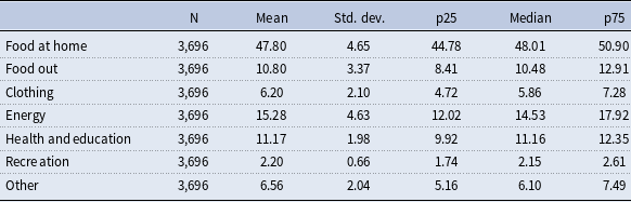
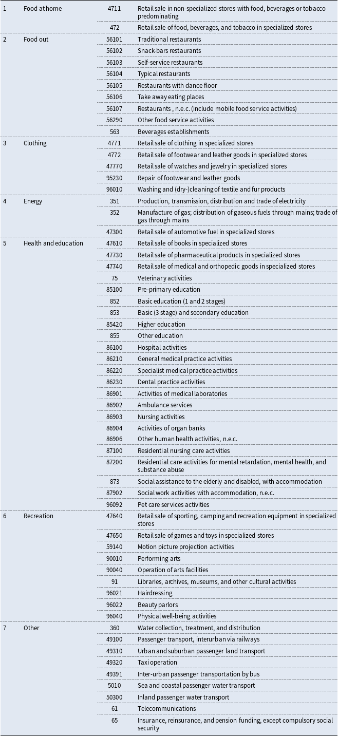
In particular, we consider 61 detailed sectors (refer to Appendix A for the detailed list). For the sake of parsimony, we manually aggregate those sectors into 7 broad groups of commodities based on their functional similarity, after analyzing the detailed description of each sector. The 7 groups are: food at home; food out; clothing; energy; health and education; recreation; other goods and services (Table 1). These commodities account for a large fraction of the non-durable consumption basket (near 80% in 2022). Moreover, the expenditure composition resulting from payments data is qualitatively similar to the one implicit in the CPI.
Budget shares of the seven commodity groups for the year 2022, in percentage
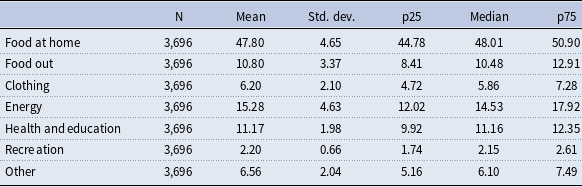
The largest budget share corresponds to food at home followed by energy, and health and education. Food out ranks next, while clothing and other goods and services (which include transportation, telecommunications, insurance, and water) have a similar weight. Finally, recreation accounts for the smallest budget share.
As payments data are disclosed on value terms only, we match a monthly price index for each of the 61 sectors. For the retail trade sectors, we use the deflators implicit in monthly retail turnover data released by Statistics Portugal. For the remaining sectors, we resort to monthly detailed CPI data (up to 5-digit level) also provided by Statistics Portugal. To obtain prices for the seven commodity groups, we start from these price indices of the 61 detailed sectors over time (common to all municipalities in a given month). At the municipality-month-sector level, we compute spending at constant prices by dividing the nominal amount of payments by the respective price index. We then aggregate both the nominal and constant price series of payments to the level of the seven commodity groups. The implicit deflator for each commodity group is obtained by dividing the two series. Thus, for each month and municipality, the weights of each sector reflect its share in total deflated expenditure of the respective commodity group. Due to this procedure, the price indices for the seven commodity groups vary across municipalities, reflecting different consumption patterns.
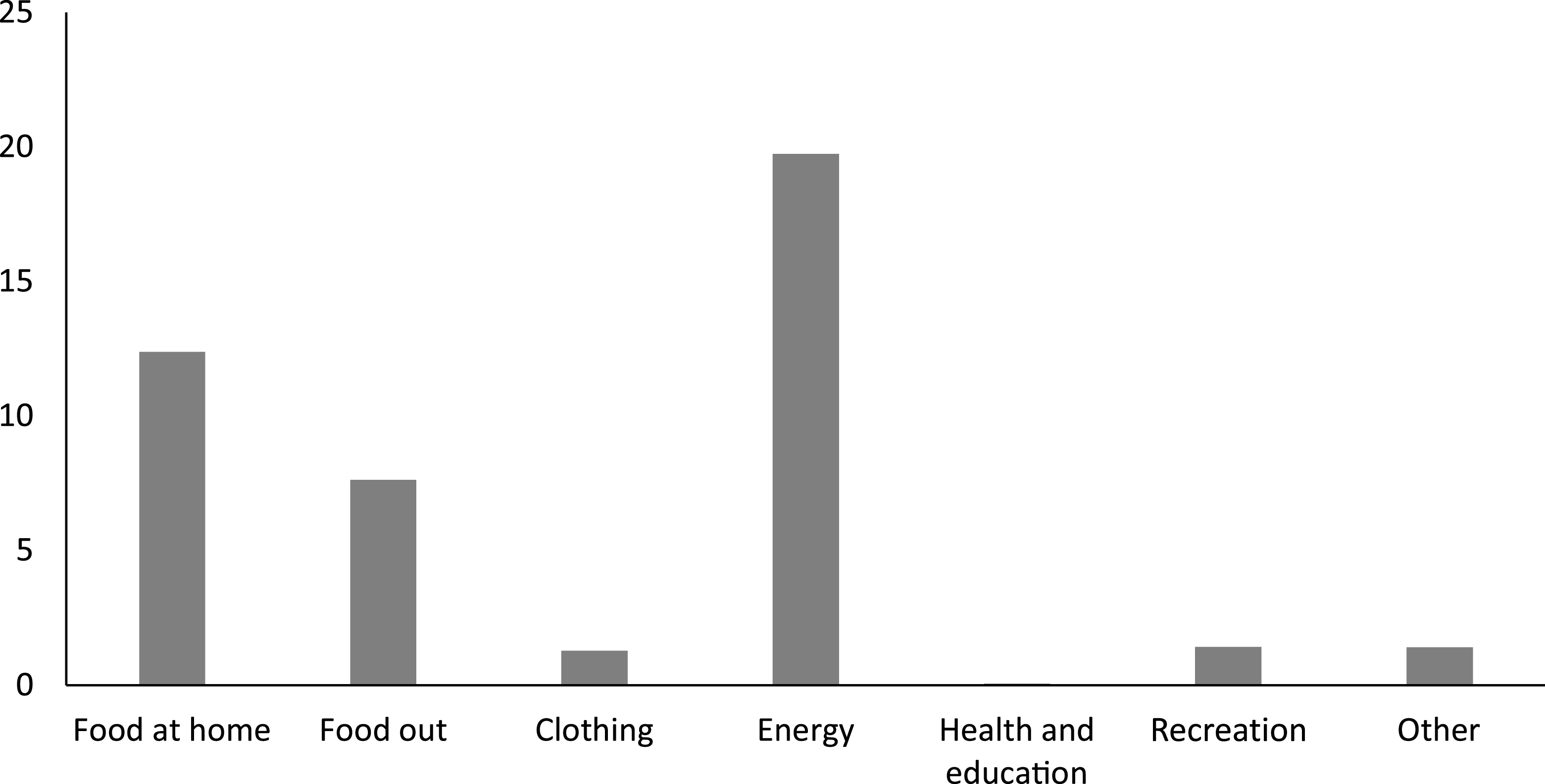
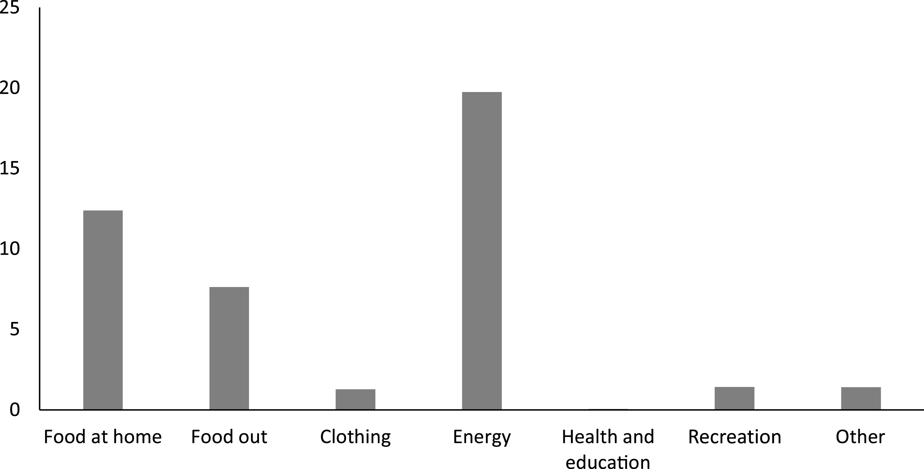
One should mention that the commodity groups that recorded the highest inflation rates were, as expected, energy, food at home, and food out, with annual changes of 19.7%, 12.4%, and 7.6%, respectively (Figure 1). In sharp contrast, the remaining commodity groups presented small price changes.
Inflation in the seven commodity groups for the year 2022, in percentage.
To obtain a per-capita measure of total nominal expenditures, we divide total monthly expenditures in the seven commodity groups by the population of each municipality, as reported by Statistics Portugal. Hence, we end up with a dataset comprising expenditure and prices for 308 consumer units, with the period under analysis running from January to December 2022 (that is, 3,696 observations). As the dataset covers the full twelve months of 2022, all welfare metrics are computed using annual averages, which mitigates potential seasonal effects; moreover, seasonal fluctuations such as sales periods in January–February and July–August are retained, as they reflect genuine price–quantity adjustments relevant to the estimated demand system.
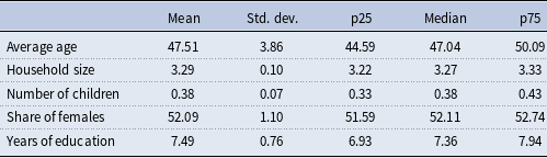
As mentioned above, we also consider a set of sociodemographic variables in the estimation of the QUAIDS model. The set of variables include age, household size, number of children per household, share of females, and years of education (Table 2). This set encompasses the commonly used demographic variables in the related literature. We draw on the population census, which provides a complete description on the size, location, and characteristics of the entire population and is conducted typically every ten years. In particular, we use the data from the Census 2021 released by Statistics Portugal and collect those variables for each municipality.
Demographic variables for the year 2021
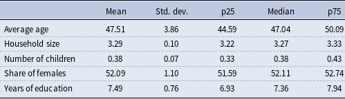
Notes: The demographic variables come from the 2021 Census and are measured at the municipality level, comprising 308 distinct units. Average age refers to the mean age of the population in each municipality. The average size of the household is computed as the ratio between the total population and the number of households in the municipality. The average number of children per household is computed as the ratio between the number of people under the age of 15 in family units and the number of households in the municipality. The share of females is the number females as a percentage of the total population. The average years of education are computed taking into account the years required to obtain the highest level of formal education, multiplied by the number of persons with such levels, and divided by the total of population of the municipality.
To instrument total expenditure, we gathered data on the after-tax household income by municipality for the year 2022, which is conveyed in the publication Income Statistics at Local Level released by Statistics Portugal. We then divided it by the population of each municipality to obtain a measure of per-capita income in each municipality. At the municipality level, the linear correlation between total per-capita expenditure and net income per capita in 2022 is 73.4%.
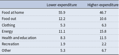
SIBS provides a breakdown of the data by quartile of average card expenditure within each municipality.Footnote 4 The SIBS quartile classification is obtained by ranking individual cards according to their total expenditure at the national level over the preceding twelve months. Based on this information, we construct two subsamples of consumers: lower- and higher-expenditure groups, defined as those below and above the national median of total spending. Each subsample contains 3,696 observations (308 municipalities observed over 12 months), as in the full sample described above. The lower- (higher-) expenditure group therefore includes only expenditure from cards in each municipality with below- (above-) median spending. Estimating separate demand systems for these two groups allows the parameters of the budget share equations to differ between lower- and higher-expenditure consumers.
In Table 3 we report the average budget shares for the two expenditure groups. Food weighs more on the consumption basket of the lower-expenditure group, whereas for the other commodity groups the shares are smaller when compared with the higher-expenditure group.
Average budget shares for lower- and higher-expenditure groups for the year 2022, in percentage
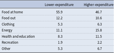
Notes: The lower-expenditure group refers to the 50% of cards with the lowest spending (at national level) over the previous 12 months in each municipality. The higher-expenditure group refers to the 50% of cards with the highest spending (at national level) over the previous 12 months in each municipality. Each group comprises 3,696 observations, 308 municipalities over 12 months.
To estimate the QUAIDS model for each consumer group and to instrument for expenditure, we collected data on after-tax household income by municipality, categorized as below or above the national median. We also gathered information on the number of fiscal aggregates in each group and municipality, both kindly provided by Statistics Portugal. The percentage share of fiscal aggregates in each group was applied to the total municipality’s population to obtain the corresponding number of individuals in each group within each municipality. Finally, the total nominal expenditure per capita for each group and municipality was calculated as described previously and then instrumented using income per capita in the separate demand system estimations.
4. Empirical analysis
4.1 QUAIDS estimation results
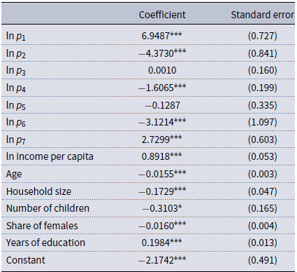
As discussed earlier, to cope with the potential endogeneity of total expenditures, a standard practice is to instrument it with income and other proxies (see, e.g., Banks et al. Reference Banks, Blundell and Lewbel1997, Blundell and Robin, Reference Blundell and Robin1999, Reference Blundell and Robin2000, Lecocq and Robin, Reference Lecocq and Robin2006, Aguiar and Bils, Reference Aguiar and Bils2015). Hence, we firstly estimate a reduced form equation for the log of total monthly per-capita expenditure considering as independent variables the identifying instrument, the log of after-tax per-capita income, as well as the seven log prices and the set of sociodemographic variables (age, household size, number of children per household, share of females, and years of education). The results are presented in Table B1 of Appendix B. We find that most variables are significant at the 1% level and the overall F-statistic from the first stage is quite high, corroborating its usefulness as expenditure instruments (
 $F(13,3682)=496.29$
).
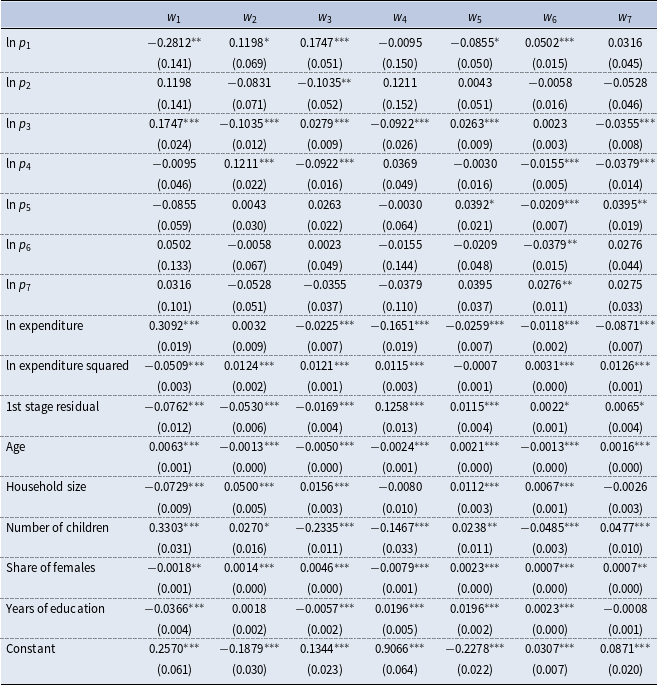
Afterward, we estimate the system of demand equations as previously described. In particular, we have as independent variables for each equation, the seven log prices, the log of total per-capita expenditure and its square, and the set of sociodemographic variables described previously. The first stage residuals of total expenditure are also added as additional regressors to the estimating equations (Hausman, Reference Hausman1978). The full set of estimation results of the budget share regressions are presented in Table 4.
Estimates of the parameters of the QUAIDS model
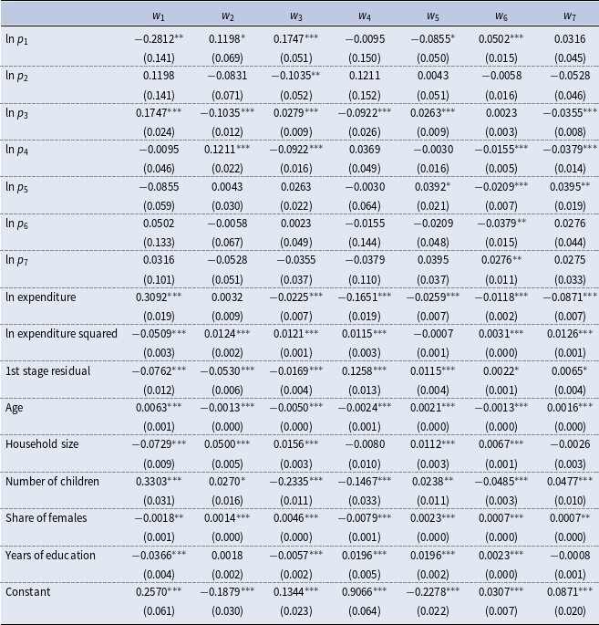
Table 4 Long description
A table showing estimates of the parameters of the QUAIDS model. The table has 20 rows and 10 columns. The columns are labeled as W1, W2, W3, W4, W5, W6, W7, ln expenditure, ln expenditure squared, 1st stage residual, Age, Household size, Number of children, Share of females, Years of education, and Constant. The rows are labeled as ln p1, ln p2, ln p3, ln p4, ln p5, ln p6, ln p7, ln expenditure, ln expenditure squared, 1st stage residual, Age, Household size, Number of children, Share of females, Years of education, and Constant. Each cell contains numerical values with standard errors in parentheses. Notable trends include significant values marked with asterisks indicating levels of statistical significance.
Notes: Estimation results of the budget share regressions of equation (8). Commodity groups: 1 “Food at home”; 2 “Food out”; 3 “Clothing”; 4 “Energy”; 5 “Health and education”; 6 “Recreation”; 7 “Other”. Number of observations: 3,696. Standard errors are in parenthesis. Stars indicate significance levels of 10% (*), 5% (**), and 1%(***).
Firstly, we find that the quadratic expenditure term is statistically significant at the 1% level for all commodities but health and education. This finding confirms the empirical adherence of the extension provided by the QUAIDS model of Banks et al. (Reference Banks, Blundell and Lewbel1997).
Secondly, we find that the residuals of the instrumental regression are significant in most cases at the 1% level (and in all equations at the 10% level). Based on the statistical significance in each equation separately as well as jointly, the null hypothesis of exogeneity of total expenditure can be rejected (
 $ {\chi }^2(6)=142.25, \hspace {0.5em} Prob \gt {\chi }^2 = 0.0000$
).
Regarding the sociodemographic variables, we find that age impacts positively the expenditure share on food at home, but negatively on food out. It also presents a positive coefficient for health and education, and for other goods and services, and a negative one for the remaining commodities. In contrast, the household size has associated a negative coefficient on the budget share for food at home, but a positive one for food out. It also presents a positive parameter for clothing, health and education, and recreation. The number of kids per household affects positively the expenditure share on food at home (and to a lesser extent food out), health and education, and other goods and services and negatively the remaining commodity groups. The share of females affects positively the share of spending on food out, clothing, health and education, recreation, and other goods and services. Finally, years of education impact positively the budget share on energy, health and education, and recreation.
4.2 Expenditure and price elasticities
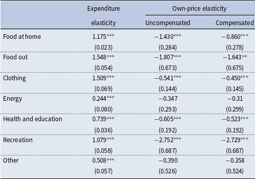
Interpreting the remaining parameters of the QUAIDS model can be challenging because the dependent variable is not the total expenditure on the commodity group or the quantity consumed but rather the budget share. A change in budget share does not necessarily indicate an increase or decrease in either total expenditure on the commodity group or the quantity consumed. Consequently, calculating expenditure and price elasticities from the coefficients obtained in the QUAIDS estimation provides a more straightforward approach to interpreting the results. The estimated expenditure and own-price elasticities are reported in Table 5.Footnote 5
Expenditure and own-price elasticities (compensated and uncompensated)
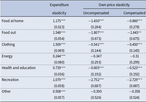
Notes: Number of observations: 3,696. Elasticities are computed at the sample mean point. Standard errors are in parenthesis. Stars indicate significance levels of 10% (*), 5% (**), and 1%(***).
Commodities with expenditure elasticities between 0 and 1 are classified as necessity goods, while those with elasticities greater than 1 are considered luxury goods. This implies that the demand for necessity goods increases less than proportionally with expenditure, whereas the demand for luxury goods increases more than proportionally. Hence, as expenditure grows, the budget share for necessities tends to decline, while the budget share for luxuries tends to rise.
We find that food at home, food out, clothing, and recreation present an expenditure elasticity above one. This means that all these group commodities can be considered luxury goods. Apart from food at home, all these commodity groups would be expected to be classified as luxuries. In the case of food at home, one should note that, for example, Lecocq and Robin (Reference Lecocq and Robin2006) report elasticities higher than one for several food items in France, with our elasticity estimate of 1.175 being within their range of estimates. All the other commodity groups can be classified as necessities, with energy displaying the lowest expenditure elasticity (as also found by Banks et al. (Reference Banks, Blundell and Lewbel1997) for the UK).
Concerning the own-price elasticities reported in Table 5, all estimated elasticities, uncompensated or compensated, have the expected negative sign, which means that an increase in the price of a commodity would lead to a decrease in its consumption demand, assuming that all other factors remain constant. If the own-price elasticity lies in the interval between −1 and 0, one can classify the commodity as price inelastic, whereas if it is lower than −1 then it can be considered price elastic.
We find that energy is the commodity group that presents the lowest (in absolute value) own-price elasticity. In addition, the null hypothesis of being zero cannot be rejected. This indicates that the demand for energy is quite price inelastic. The same happens with other goods and services, which includes transportation, telecommunications and water. Health and education can also be classified as price inelastic, but the estimated elasticities are statistically different from zero. In contrast, food out and recreation are the commodity groups with larger own-price elasticities (in absolute terms) being highly responsive to changes in their prices.
One should also mention that although the estimated compensated elasticities are higher than the uncompensated ones, as expected from equation (14), they are not that different. Only in the case of food at home the difference is larger, with the uncompensated elasticity being lower than −1, while the compensated elasticity is higher than −1.
Finally, before moving to the welfare analysis of the inflation shock, we evaluate the theoretical regularity conditions of positivity, monotonicity, and curvature using the estimated parameters and the data (see Barnett and Serletis, Reference Barnett and Serletis2008 and Serletis and Shahmoradi, Reference Serletis and Shahmoradi2007). In our application, positivity and monotonicity hold for all observations in the sample, indicating non-negative estimated budget shares and indirect utility that is increasing in total expenditure. Curvature is assessed by examining the negative semidefiniteness of the Slutsky substitution matrix, the standard necessary and sufficient condition for concavity of preferences in prices. Using an observation-specific evaluation of the Slutsky matrix, we find that this condition does not hold in the sample. To understand the source of these violations, we decompose the Slutsky quadratic form and identify the goods and substitution channels contributing most to the failure of concavity. The results indicate that the violations arise almost entirely from a single cross-price interaction, namely between good 1 (Food at home) and good 3 (Clothing). All other own- and cross-price components contribute little to the observed violations and are consistent with concavity throughout the sample.Footnote 6 This caveat does not undermine the overall usefulness of the estimated demand system for policy analysis, but estimated cross-price elasticities between these two goods should be interpreted with caution as local approximations rather than as globally valid substitution relationships.
4.3 Welfare cost of the inflation episode on consumers
As discussed earlier, the estimation of a demand system enables measuring changes in welfare due to exogenous variations in prices. Price shocks can occur for several reasons and policymakers may want to assess their impact on welfare either ex post or ex ante. In this respect, for instance, Banks et al. (Reference Banks, Blundell and Lewbel1997) simulate a tax reform comprising the imposition of a 17.5% sales tax on clothing in the UK; and Tóth et al. (Reference Tóth, Cupák and Rizov2021) evaluate a VAT tax cut of 10 percentage points (from 20% to 10%) for certain basic food categories in Slovakia. In what follows, we use our estimated QUAIDS model to quantify the welfare cost of the 2022 inflation episode for Portuguese consumers.
Recall from Section 2.2 that the CV is defined as
 $CV = m - e(p^1, v^0)$
. To calculate the CV associated with the 2022 inflation episode, we must first specify the two price vectors,
 $p^1$
and
 $p^0$
, used as inputs to the expenditure function.
 $p^1$
denotes the observed 2022 prices for every municipality–commodity–month combination, that is, for each municipality
 $h$
, commodity group
 $i$
and month
 $t$
,
 $p^1(h,i,t)$
is the realized price in 2022.
 $p^0$
represents the counterfactual price vector in which every commodity’s price is fixed at its 2021 municipality-specific average. That is, for each municipality
 $h$
and commodity
 $i$
,
 $p^0(h,i)$
equals the arithmetic mean of the monthly prices in 2021 of commodity
 $i$
and is held constant throughout the analysis.
Using the estimated QUAIDS parameters together with the price vectors
 $p^1$
and
 $p^0$
, we compute the CV for each municipality and month to quantify the welfare cost of this inflation episode. Intuitively, when prices move from
 $p^0$
to
 $p^1$
, a consumer would need to spend more to attain the same level of utility as in the absence of the price change. The CV thus represents this monetary shortfall, the amount required to restore the original level of utility. Because CV is negative under our definition, we report its absolute value in the figures for readability. Since our data are monthly, the CV is computed at a monthly frequency as well. To facilitate the presentation and abstract from potential seasonality, we aggregate monthly CVs to an annual measure by summing the monthly values and then expressing the result both in euros per year and as a percentage of each municipality’s annual per-capita expenditure.
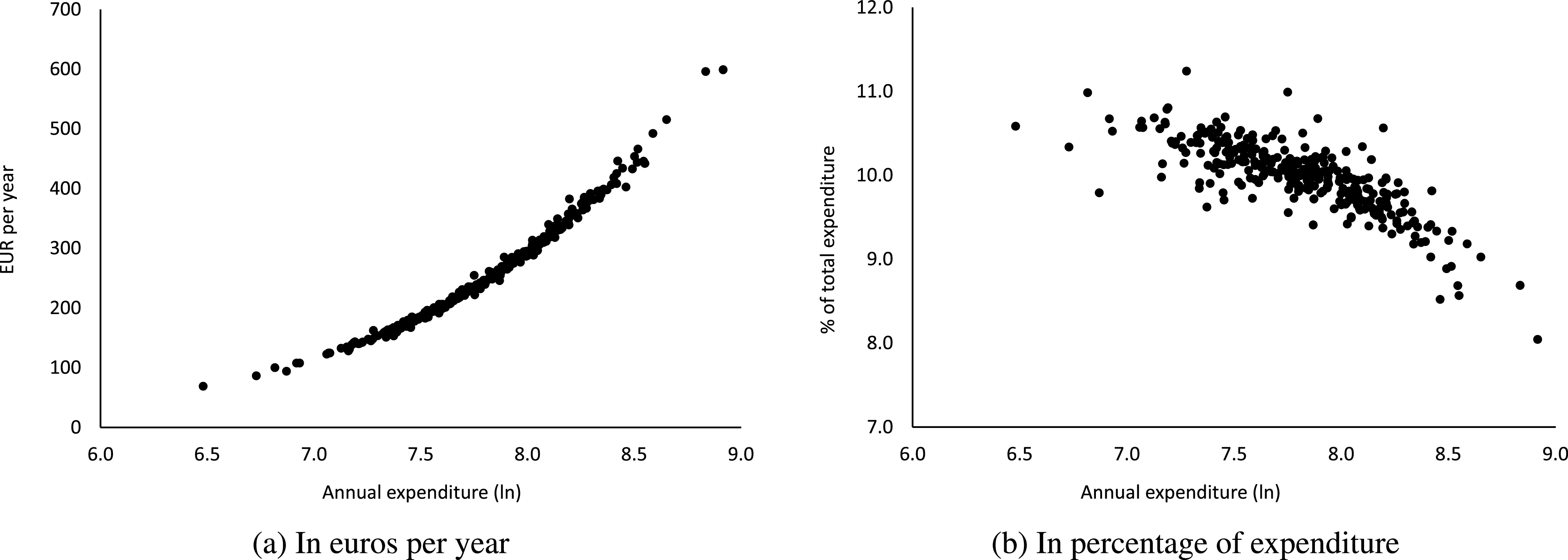
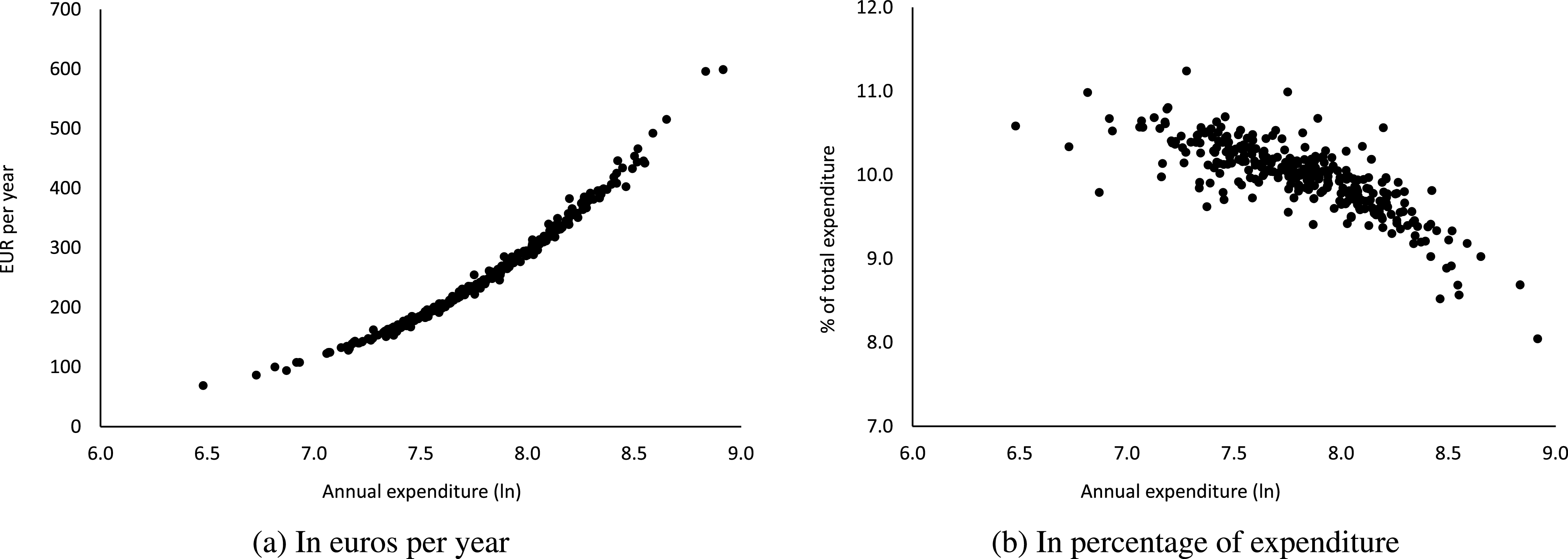
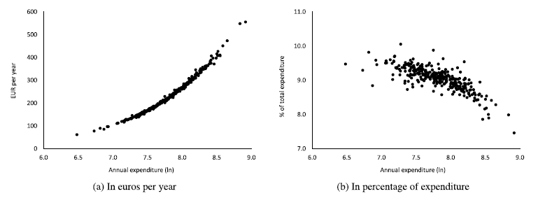
Panel A of Figure 2 illustrates the welfare loss by plotting the CV measured in euros per year for the 308 municipalities against the log of total annual per-capita expenditure. As expected, all consumer units experienced a welfare loss, which increases with total expenditure (see also Banks et al. (Reference Banks, Blundell and Lewbel1997)). The average of the CV is 259 euros.Footnote 7
The previous analysis is based on absolute terms, that is, in euros. However, it is also relevant to assess how much the welfare cost of inflation represents over annual per-capita expenditure. This type of analysis allows to shed light on the progressivity or regressivity of the inflation tax. When we assess the welfare loss in percentage of the total expenditure, we find that the welfare cost decreases as total expenditure increases (Figure 2, panel B). This means that the lower-expenditure consumers underwent a relatively larger welfare loss than higher-expenditure consumers, a regressive effect.Footnote 8
Welfare loss based on compensating variation (CV).
Notes: Panel A depicts the annual CV in EUR per year for each of the 308 consumer units and panel B in percentage of total annual per-capita expenditure. For readability, we present the absolute values of CV (the metric is negative in all cases).
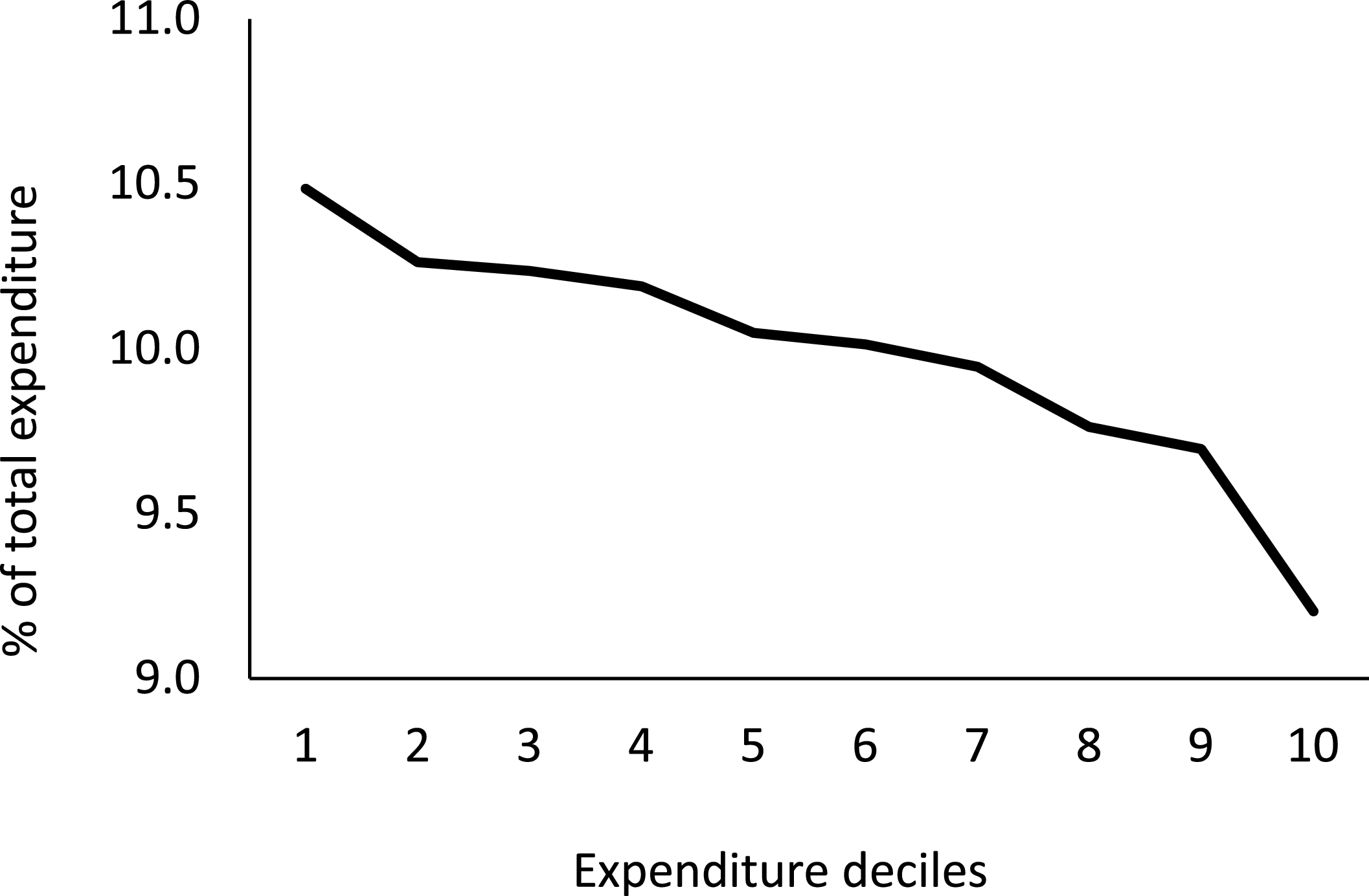
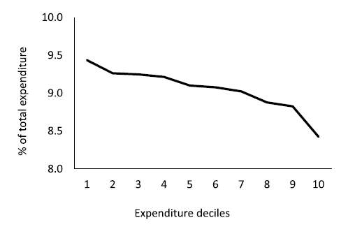
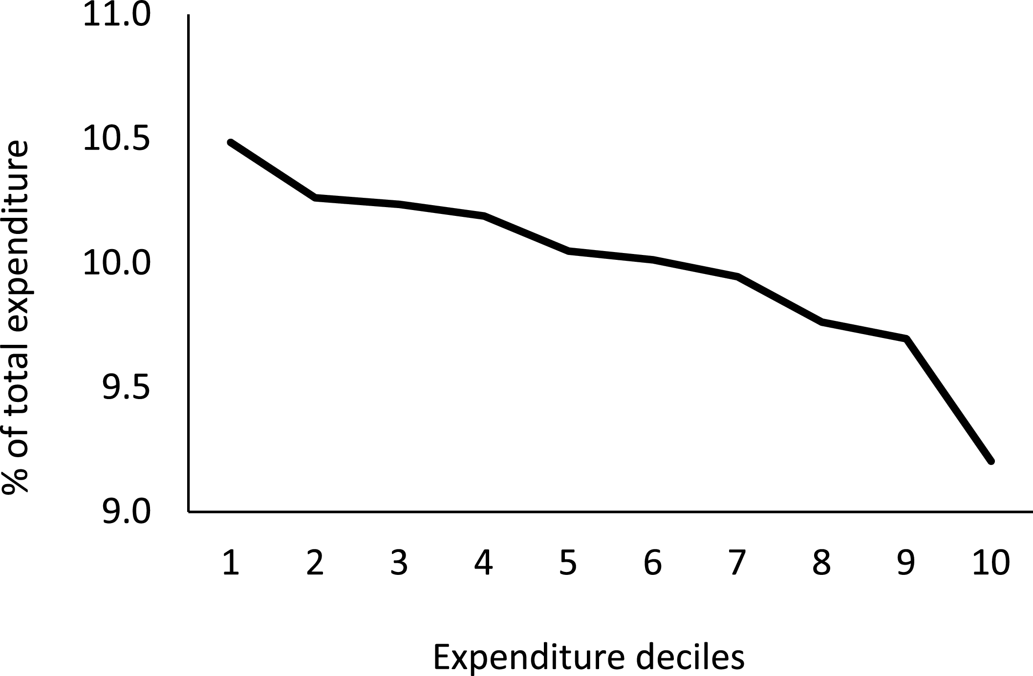
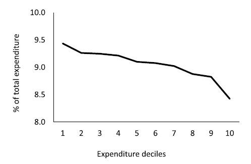
To enhance clarity on the distributional impact of inflationary shocks, Figure 3 plots the welfare cost, as a proportion of total expenditure, across expenditure deciles. The annual average CV is 10% of total expenditure, but there is a noteworthy heterogeneity across expenditure levels. The lowest expenditure decile underwent a welfare loss of 10.5% of total expenditure, whereas the highest decile recorded a welfare loss of 9.2%.Footnote 9 Hence, households with lower budgets had, in relative terms, a larger welfare loss than higher-expenditure households as a result of the inflation shock observed in 2022.
Welfare loss based on compensating variation (CV), in percentage of total expenditure.
Notes: Average values of the CV (in percentage of total expenditure) in each decile of total annual per-capita expenditure. For readability, we present the absolute values of CV (the metric is negative in all cases).
To better understand the mechanisms behind the observed distributional patterns of welfare losses, we complement the CV baseline analysis with a set of benchmark comparisons reported in Appendix E. We begin by comparing the QUAIDS-based CV with a simple share-weighted price index that captures only differences in inflation exposure. We then conduct two post-estimation calibration exercises that selectively shut down cross-price substitution effects and the nonlinear Engel-curve component of the model. Taken together, these exercises show that the heterogeneity in welfare losses does not appear to be primarily driven by differences in inflation exposure or substitution patterns, but instead by the non-homothetic structure of the Engel curves. This highlights the importance of allowing expenditure-dependent behavioral responses when assessing the distributional impact of large and uneven price shocks like the one observed in 2022.
5. Further differentiating lower- and higher-expenditure consumers
In the previous section, we estimated a demand system for the average consumer in each municipality, comprising both high- and low-expenditure consumers, which yielded a set of representative expenditure and price elasticities. In this section, we estimate two separate QUAIDS models for the average of the lower- and higher-expenditure consumers in each municipality. As described in Section 3, for each municipality we have data on card payments of consumers with below- and above-median spending. Accordingly, we partition the dataset into two parallel subsamples, namely low-spending and high-spending consumers within each municipality. Each subsample contains 308 municipalities observed over 12 months, and we estimate separate QUAIDS models for the two groups. For example, the low-spending group includes only households in each municipality whose expenditure is below the national median. This approach allows the budget share parameters to differ across groups, providing additional flexibility to assess whether demand responses vary systematically along the expenditure distribution, beyond the nonlinear Engel-curve effects captured by the baseline QUAIDS model in the previous section.
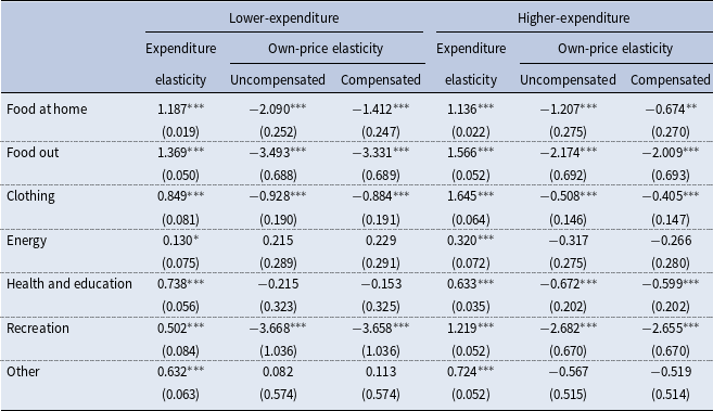
Table 6 reports the estimated elasticities for the lower- and higher-expenditure consumers. Concerning the expenditure elasticities, the estimates are broadly similar across the two consumer groups except for clothing and recreation. In these two cases, for the lower-expenditure group the estimated elasticities are below one, suggesting that these commodities are necessities. In contrast, for the higher-expenditure consumers, the estimated values are above one indicating that they are luxuries.
Expenditure and own-price elasticities (compensated and uncompensated)
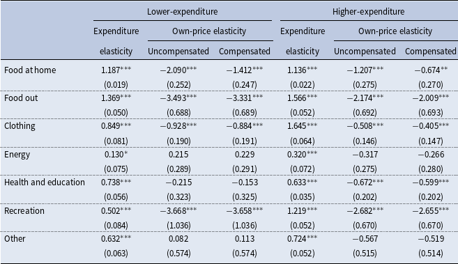
Table 6 Long description
A table with six rows and four columns comparing expenditure and own-price elasticities for lower- and higher-expenditure consumers. The columns are labeled Expenditure elasticity, Uncompensated own-price elasticity, and Compensated own-price elasticity for both lower- and higher-expenditure groups. The rows are labeled with different categories: Food at home, Food out, Clothing, Energy, Health and education, Recreation, and Other. Each cell contains numerical values representing the elasticities. Notable trends include lower expenditure elasticities for clothing and recreation in the lower-expenditure group, indicating these are necessities, while higher expenditure elasticities for the same categories in the higher-expenditure group, indicating luxuries.
Notes: Number of observations: 3,696 in each demand system. Elasticities are computed at the sample mean point. Standard errors are in parenthesis. Stars indicate significance levels of 10% (*), 5% (**), and 1%(***).
Regarding own-price elasticities, one should note the following. Firstly, as found in the previous section, the demand is quite price inelastic in the cases of energy, health and education, and other goods and services. In fact, the estimated elasticities of these commodities are not statistically different from zero for both lower- and higher-expenditure consumers, except for health and education for the latter group where the elasticity is negative but still below 1 in absolute value.
For all the other commodity groups, we find that lower-expenditure consumers present larger elasticities (in absolute value) than higher-expenditure consumers. In particular, for food (either at home or out), clothing, and recreation, the estimated elasticities (either uncompensated or compensated) for lower-expenditure consumers are larger, in absolute value, than for higher-expenditure consumers. That is, the price response for consumers with a smaller budget is more pronounced than for those with higher income. This is in line with Lewbel and Pendakur (Reference Lewbel and Pendakur2009) who argue that the poor substitute more than the rich, as well as with the recent empirical evidence of Auer et al. (Reference Auer, Burstein, Lein and Vogel2024) who find that lower-income households have higher price elasticities leading to unequal welfare effects of import price shocks in Switzerland. In addition, Bobasu et al. (Reference Bobasu, Charalambakis and Kouvavas2024) document, based on the ECB’s Consumer Expectations Survey data, that households facing budget constraints were more likely to adjust their consumption patterns compared with households with unconstrained budgets during the latest inflationary episode.
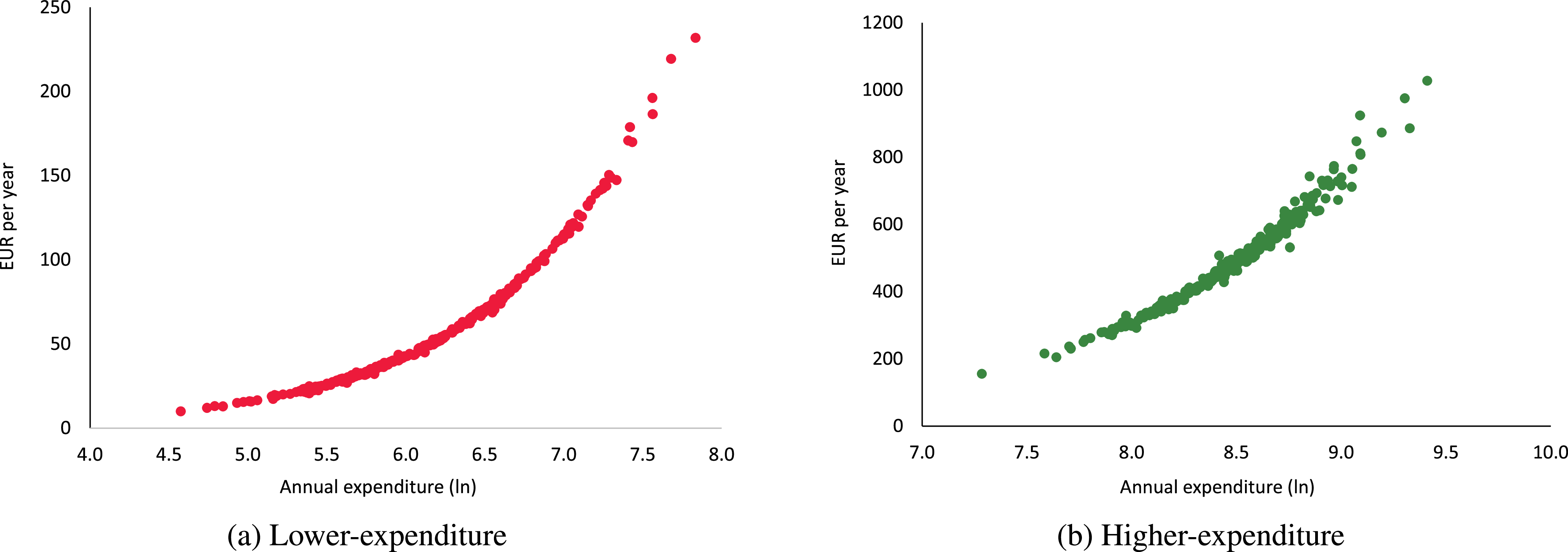
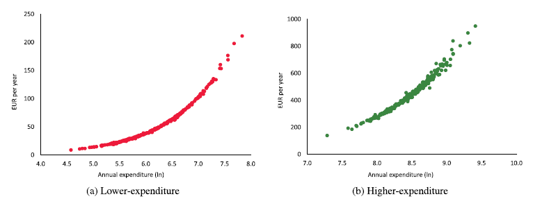
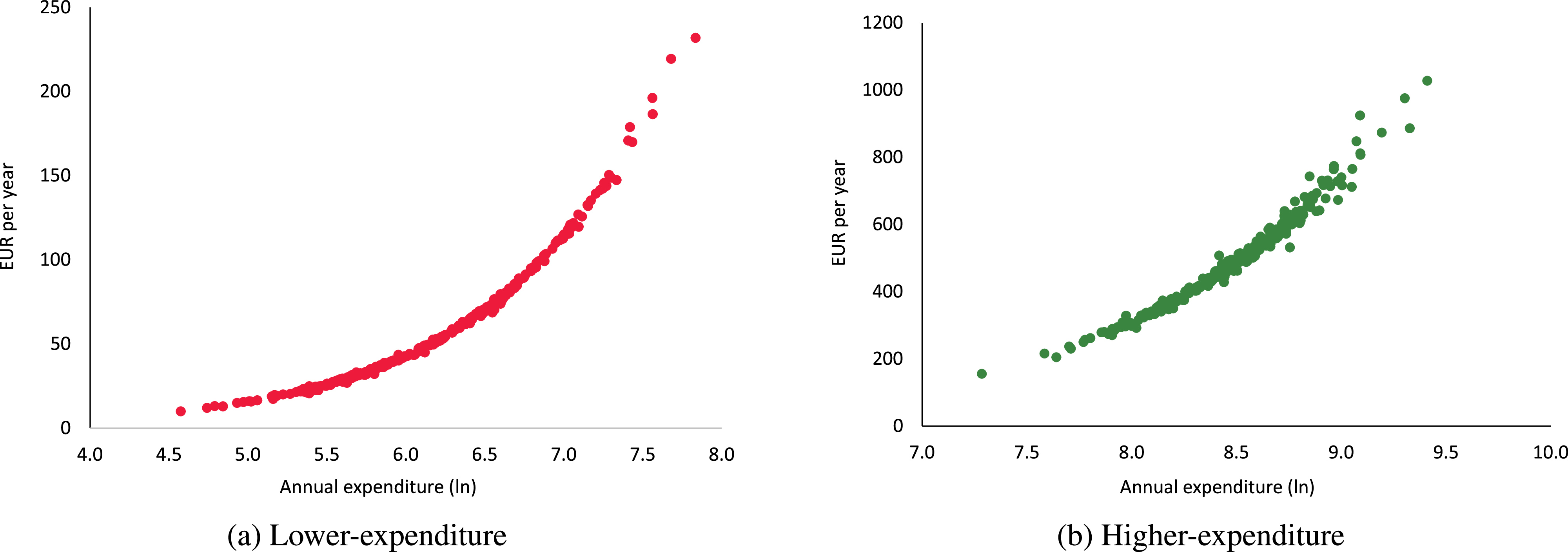
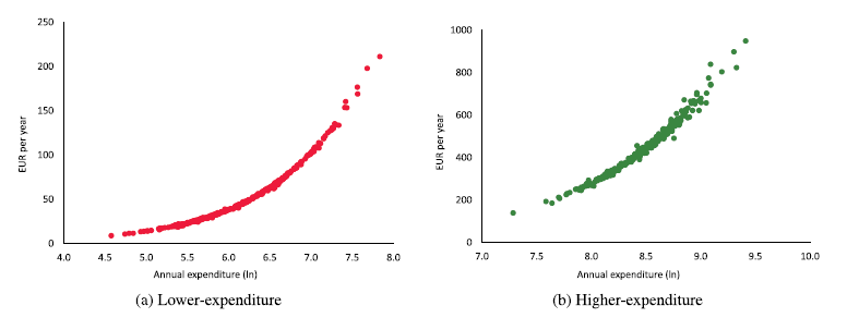
Given the estimated QUAIDS parameters for lower- and higher-expenditure consumers, one can further differentiate the welfare cost of the inflation episode. Figure 4 presents the annual CVs in euros per year for the 308 consumer units on each group. As before, we find that, either lower- or higher-expenditure consumers, all units had a welfare loss, which increases with total expenditure.Footnote 10
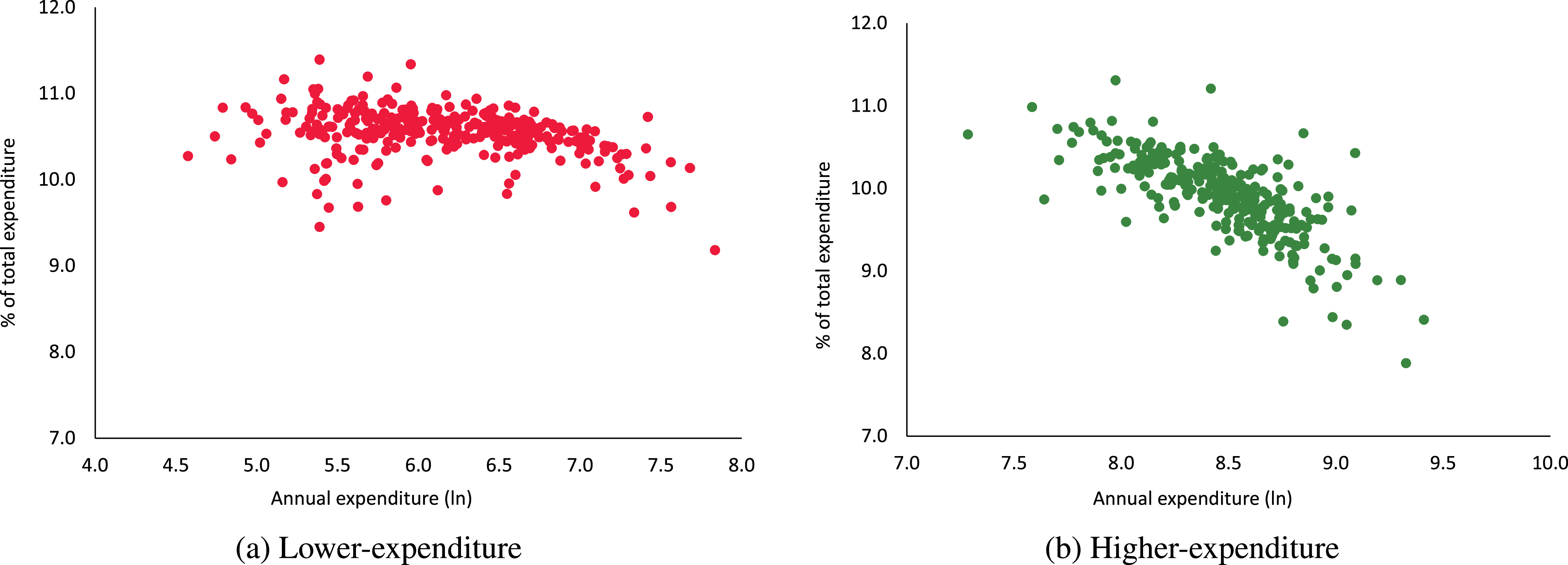
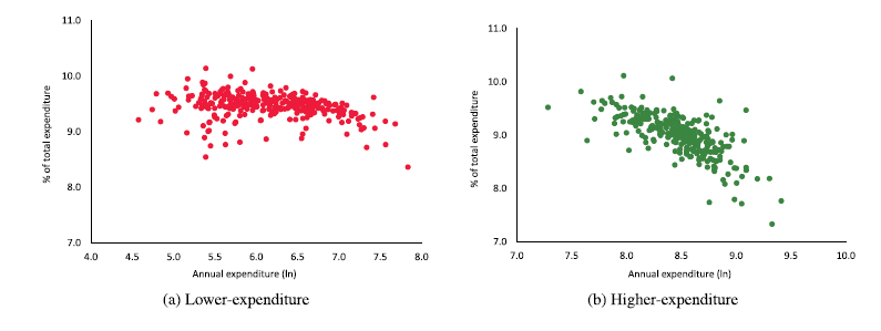
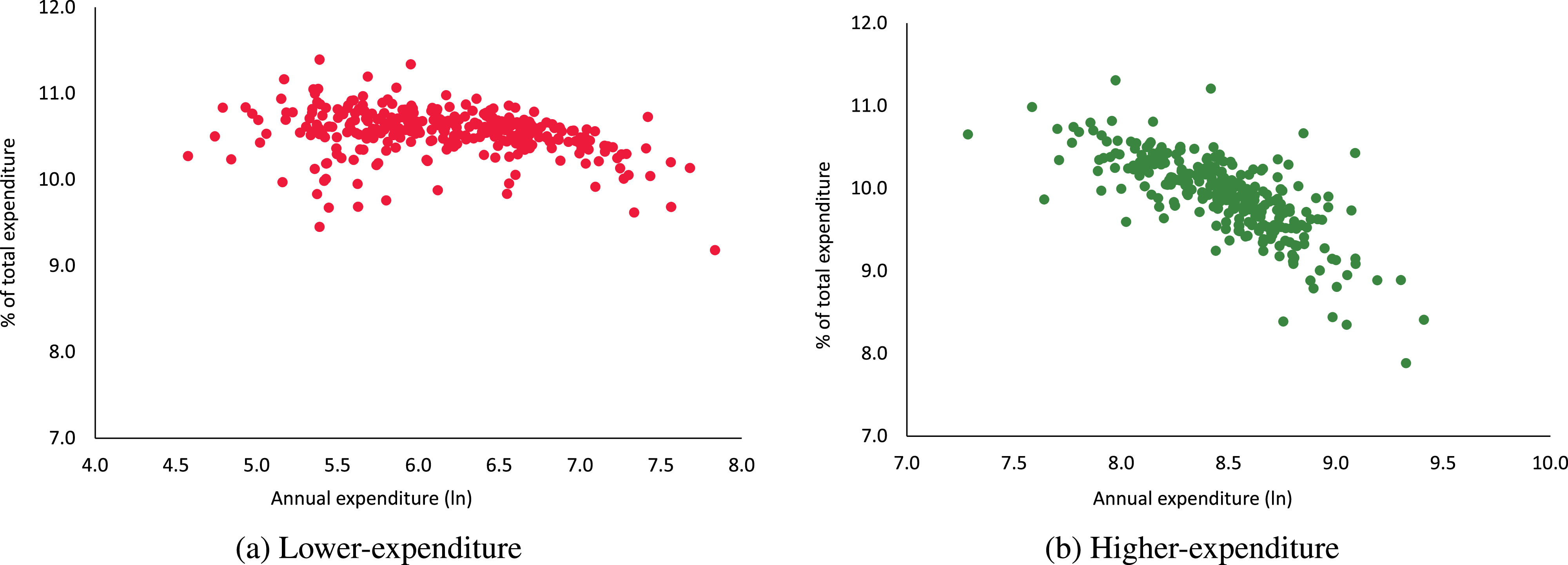
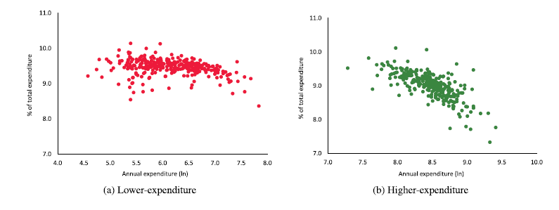
When the welfare cost is evaluated in percentage of total expenditure (Figure 5), the loss for lower-expenditure consumers hovers around 10.5%. In contrast, there is more heterogeneity among higher-expenditure consumers, with a clear decreasing pattern as expenditure rises. For the lowest decile among the higher-expenditure consumers, the welfare loss amounts to 10.5%, whereas for the highest decile, the welfare cost is less than 9.3%. Hence, although there is no major inequality among the lower-expenditure consumers, the differences are much larger within the higher-expenditure group.
Welfare loss based on compensating variation (CV).
Notes: Annual CV in EUR per year for each of the 308 consumer units on each group. For readability, we present the absolute values of CV (the metric is negative in all cases).
Welfare loss based on compensating variation (CV), in percentage of total expenditure.
Notes: Annual CV in percentage of total annual per-capita expenditure for each of the 308 consumer units on each group. For readability, we present the absolute values of CV (the metric is negative in all cases).
6. Conclusions
After an extended period of low and stable inflation in developed countries, prices rose gradually in the aftermath of the COVID-19 pandemic before experiencing a dramatic increase with the onset of the war in Ukraine in February 2022. This surge was abrupt and primarily driven by international food and energy prices, leading to inflation peaking in many European countries toward the end of 2022.
In this paper, we examine the heterogeneous and unequal welfare costs of inflation, using the recent inflationary episode as a case study. We quantify the welfare impact of the substantial relative price changes on consumers of a small open European economy. We focus on Portuguese consumers by using electronic payments data to capture changing spending patterns during 2022.
We estimate a demand system, specifically a QUAIDS model, to infer expenditure and price elasticities for seven commodity groups. Our findings reveal that food (both at home and out), clothing, and recreation exhibit expenditure elasticities greater than one, while health and education, energy, and other goods and services are classified as necessities. All own-price elasticities are negative. Notably, the identified commodity groups classified as necessities are also characterized by price inelasticity.
Using the estimated QUAIDS parameters, we quantify the welfare cost of the inflationary episode. We find that the average CV is around 10% of total expenditure, with significant heterogeneity across expenditure levels. Lower-expenditure consumers experience a relatively larger welfare loss compared to those with higher expenditure, underscoring the distributive effects of the inflation shock and its regressive nature.
To further investigate this issue, we estimate separate demand systems for lower- and higher-expenditure consumer groups. Our findings indicate that lower-expenditure consumers generally exhibit larger own-price elasticities compared to their higher-expenditure counterparts. Given the two different sets of estimated parameters, we can more thoroughly assess welfare costs within each group. For lower-expenditure consumers, the welfare cost hovers around 10.5% of total expenditure. In contrast, higher-expenditure consumers show more heterogeneity, with a clear downward trend in welfare costs as expenditure increases. Overall, our findings highlight the need for policy frameworks that address the unequal impacts of inflation, ensuring support measures are targeted toward the most affected consumer groups.
Acknowledgements
The authors are grateful to the co-editor, Apostolos Serletis, and two anonymous referees for their helpful comments and suggestions. The analyses, opinions, and findings expressed in this article are those of the authors and do not necessarily coincide with those of Banco de Portugal or the Eurosystem. Any errors and omissions are the sole responsibility of the authors.
Appendix
A. Definition of the commodity groups
Detailed description of the seven groups of commodities
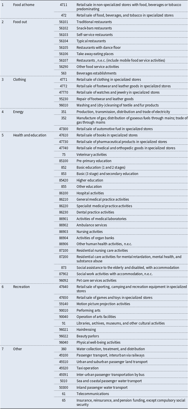
Notes: The codes refer to the Portuguese industrial classification CAE-Rev 3.
B. Instrumental regression
First-stage expenditure estimates
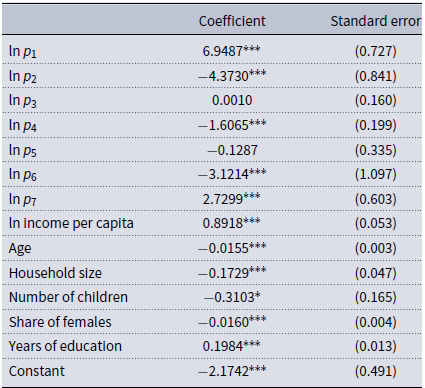
Table B1 Long description
A table with 8 columns and 8 rows showing first-stage expenditure estimates. The columns are labeled as Food at home, Food out, Clothing, Energy, Health and education, Recreation, and Other. The rows are labeled similarly. Each cell contains a value and a significance level in parentheses. Notable values include strong negative correlations like -0.860 between Food at home and itself, and strong positive correlations like 3.306 between Clothing and itself. The table provides a detailed view of how different expenditure categories relate to each other.
Notes: The dependent variable is the logarithm of monthly total per-capita expenditure. Commodity groups: 1 “Food at home”; 2 “Food out”; 3 “Clothing”; 4 “Energy”; 5 “Health and education”; 6 “Recreation”; 7 “Other”. Standard errors are in parenthesis. Number of observations: 3,696. Stars indicate significance levels of 10% (*), 5% (**), and 1%(***).
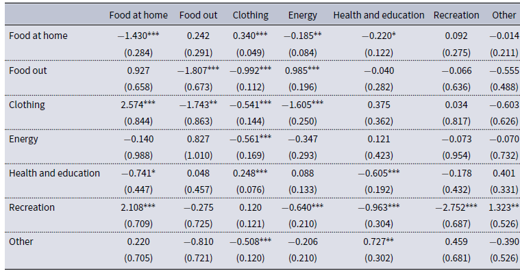
C. Own- and cross-price elasticities of demand
Uncompensated own- and cross-price elasticities
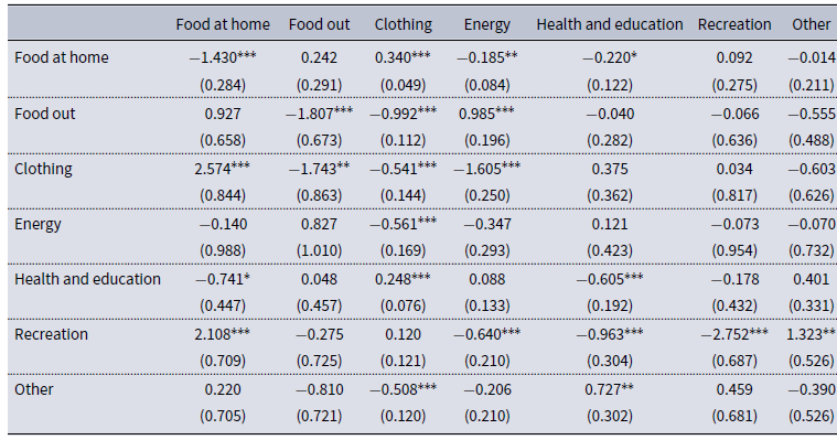
Notes: Number of observations: 3,696. Elasticities are computed at the sample mean point. Standard errors are in parenthesis. Stars indicate significance levels of 10% (*), 5% (**), and 1%(***).
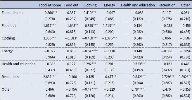
Compensated own- and cross-price elasticities
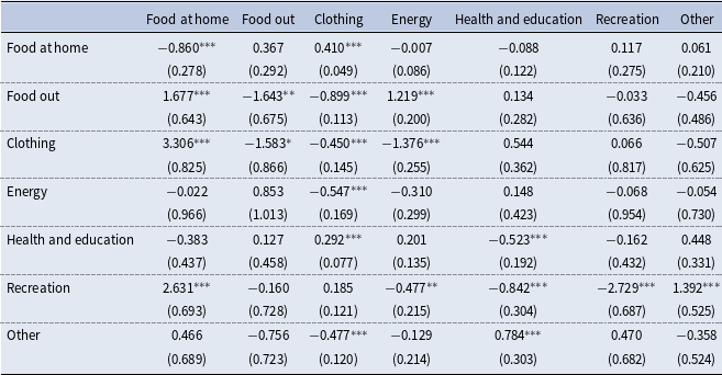
Notes: Number of observations: 3,696. Elasticities are computed at the sample mean point. Standard errors are in parenthesis. Stars indicate significance levels of 10% (*), 5% (**), and 1%(***).
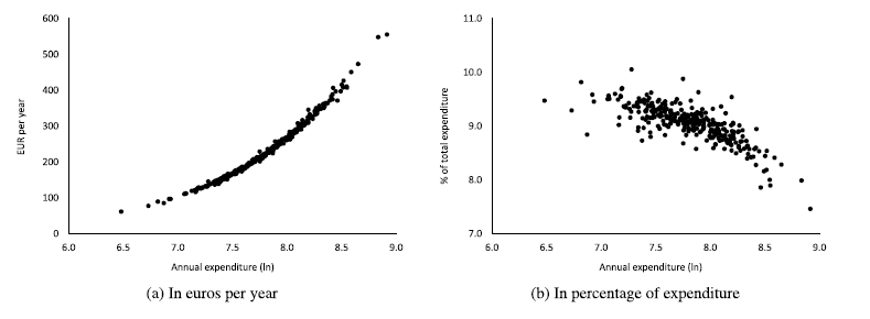
D. Equivalent variation
Welfare loss based on equivalent variation (EV).
Notes: Panel A depicts the annual EV in EUR per year for each of the 308 consumer units and panel B in percentage of total annual per-capita expenditure. For readability, we present the absolute values of EV (the metric is negative in all cases).
Welfare loss based on equivalent variation (EV), in percentage of total expenditure.
Notes: Average values of the EV (in percentage of total expenditure) in each decile of total annual per-capita expenditure. For readability, we present the absolute values of EV (the metric is negative in all cases).
Welfare loss based on equivalent variation (EV).
Notes: Annual EV in EUR per year for each of the 308 consumer units on each group. For readability, we present the absolute values of EV (the metric is negative in all cases).
Welfare loss based on equivalent variation (EV), in percentage of total expenditure.
Notes: Annual EV in percentage of total annual per-capita expenditure for each of the 308 consumer units on each group. For readability, we present the absolute values of EV (the metric is negative in all cases).
E. Benchmark comparisons of the CV
This appendix includes a set of benchmark exercises to compare with our baseline measure of CV derived from the QUAIDS model. First, we compute a log-geometric price index using municipality-specific budget shares fixed in the same month of the previous year and the corresponding log price changes of the seven commodity groups.
Second, we perform two post-estimation calibration exercises that selectively shut down channels in the estimated QUAIDS model: (i) eliminate cross-price substitution by imposing
 $\gamma _{ij}=0$
for all
 $i\neq j$
; (ii) remove the nonlinear Engel-curve component by setting
 $\lambda _i=0$
for all
 $i$
. All counterfactual CVs are computed using the baseline estimated parameters and the same pre- and post-shock price vectors used in the main analysis.
As a first benchmark, we consider a simple price index based on a share-weighted average of log price changes. For each municipality
 $h$
and month
 $t$
, the index is defined as:
 \begin{equation} \pi _{h,t} = \sum _{i=1}^{N} w_{h,i,t-12} \, \Delta \ln p_{h,i,t}, \end{equation}
where
 $w_{h,i,t-12}$
denotes the expenditure share of good
 $i$
in municipality
 $h$
in the same month of the previous year, and
 $\Delta \ln p_{h,i,t} = \ln p_{h,i,t} - \ln p_{h,i,t-12}$
is the corresponding log price change.
The annual price index for each municipality is obtained by averaging the monthly values:
 \begin{equation} \pi _{h} = \frac {1}{12} \sum _{t=1}^{12} \pi _{h,t} \end{equation}
This measure corresponds to a log-geometric index with lagged shares. Intuitively, if all households had kept their 2021 budget shares fixed, the cost of living would have increased by this amount. It captures differences in inflation exposure arising from disparities in expenditure composition across municipalities. As such, this index can be interpreted as an exact cost-of-living index under preferences consistent with a Cobb–Douglas structure. In contrast, the CV derived from the QUAIDS model allows both expenditure shares and substitution patterns to adjust endogenously to price changes, with responses that vary according to the level of total expenditure.
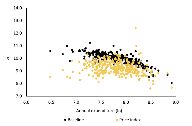
The resulting average annual inflation rate across municipalities is 9.3% in 2022, compared with a welfare cost of roughly 10% of total expenditure. Figure E1 compares the municipality-level annual average log price changes with the CV, expressed as a percentage of per-capita expenditure, shown in panel B of Figure 2. Although the average level of the index of log price changes is broadly similar to the average annual CV, the decreasing pattern across the expenditure distribution is less pronounced. The linear correlation between the two annual municipality-level series is 42.4%.
Welfare loss based on compensating variation (CV), in percentage of total expenditure, and log-geometric index of price changes.
Notes: The CV values correspond to those reported in panel B of Figure 2. The price index values represent, for each municipality, the annual average of monthly share-weighted log price changes, where the expenditure shares correspond to those of the same month in the previous year.
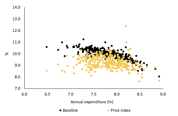
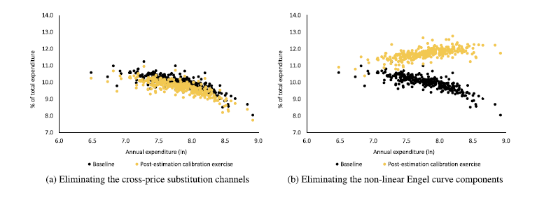
Figure E2 presents the results of the two post-estimation calibration exercises based on the estimated QUAIDS parameters. Panel A reports the results obtained after eliminating cross-price substitution effects, by setting
 $\gamma _{ij}=0$
for all
 $i \neq j$
, while leaving all other parameters unchanged. The resulting welfare measures are very close to the baseline estimates: the average CV is 9.7% of total expenditure, and the cross-municipality variation is largely preserved, with a correlation of 99% with the baseline CV. This suggests that cross-price substitution effects play a limited role in shaping both the level and the distribution of welfare losses in our setting.
Panel B reports the results obtained after eliminating the nonlinear Engel-curve component of the model, by setting
 $\lambda _i = 0$
for all
 $i$
, while leaving all other parameters unchanged. In this case, the average CV increases to 11.7% of total expenditure, and the gradient of welfare losses across the expenditure distribution changes markedly, with a slightly negative correlation with the baseline CV (-6%). This indicates that the non-homotheticity captured by the QUAIDS specification appears to play a central role in shaping the distributional pattern of welfare effects.
Taken together, these findings underscore the value of a structural demand-system approach in our setting: allowing expenditure-dependent behavioral responses is essential to capture the distributional consequences of large and uneven price shocks like the ones observed in 2022.
Welfare loss based on compensating variation (CV), in percentage of total expenditure.
Notes: The baseline results are those included in panel B of Figure 2. In panel A, the results of the post-estimation calibration exercise are obtained using the estimated parameters of the baseline QUAIDS specification but setting all cross-price parameters to zero, that is, imposing
 $\gamma _{ij}=0$
for all
 $i \neq j$
. In panel B, the results of the post-estimation calibration exercise are obtained using the estimated parameters of the same QUAIDS specification but setting
 $\lambda _i = 0$
for all
 $i$
, that is, removing the quadratic term in log expenditure.
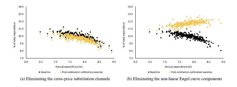
Figure E2. Long description
Two scatter plots compare the percentage of total expenditure against annual expenditure in natural logarithm scale, showing baseline and post-estimation calibration exercise results. Panel A: Eliminating the cross-price substitution channels. The scatter plot shows the percentage of total expenditure on the vertical axis ranging from 7.0 to 14.0 percent and annual expenditure in natural logarithm on the horizontal axis ranging from 6.0 to 9.0. Black dots represent baseline results, and yellow dots represent post-estimation calibration exercise results. The trend shows a general decrease in the percentage of total expenditure as annual expenditure increases. Panel B: Eliminating the non-linear Engel curve components. The scatter plot shows the percentage of total expenditure on the vertical axis ranging from 7.0 to 14.0 percent and annual expenditure in natural logarithm on the horizontal axis ranging from 6.0 to 9.0. Black dots represent baseline results, and yellow dots represent post-estimation calibration exercise results. The trend shows a general decrease in the percentage of total expenditure as annual expenditure increases.

 γij=0
 i≠j
 λi=0
 i


