




1. Introduction
Massive stars exhibit unique physical processes, including strong winds and eruptive outbursts (e.g., Davidson & Humphreys Reference Davidson and Humphreys2012; Vink Reference Vink2015; Kashi et al. Reference Kashi, Davidson and Humphreys2016; Schneider et al. Reference Schneider, Podsiadlowski and Laplace2024; Maryeva Reference Maryeva2024). These stars are characterized by high mass loss rate winds, which become more intense as they evolve (e.g., Krtička & Kubát Reference Krtička and Kubát2006; Vink Reference Vink2022; Curé & Araya Reference Curé and Araya2023; Krtička et al. Reference Krtička, Kubát and Krtičková2025). Many massive stars are part of binary and multiple systems (Vanbeveren et al. Reference Vanbeveren, De Donder, Van Bever, Van Rensbergen and De Loore1998; Sana et al. Reference Sana, de Mink and de Koter2012; Sana et al. Reference Sana, Shenar and Bodensteiner2025). Evolutionary stages such as the Luminous Blue Variable (LBV) and Wolf-Rayet (WR) stages, are often attributed to binary evolution with mass exchange rather than single star evolution paths (e.g., Kashi & Soker Reference Kashi and Soker2010; Mahy et al. Reference Mahy, Lanthermann and Hutsemékers2022; Aghakhanloo et al. Reference Aghakhanloo, Smith and Andrews2022; Lobel & Gorlova Reference Lobel and Gorlova2025).
In binary systems with two stars ejecting winds, these winds collide, forming a colliding wind structure (CWS) (e.g., Stevens et al. Reference Stevens, Blondin and Pollock1992; Eichler & Usov Reference Eichler and Usov1993). Its apex is usually near this line, divided by a contact discontinuity with shock waves on either side. The shocked gas flows asymptotically along the cone sides close to the stars, where we focus our simulation and discussion. The primary parameter influencing the contact discontinuity shape and the CWS is the momentum ratio of the winds
 $ \eta={\dot{M}_2 v_2}/{\dot{M}_1 v_1}$
, where
 $\dot{M}_2$
and
 $v_2$
are the mass loss rate and wind velocity of the secondary star, and
 $\dot{M}_1$
and
 $v_1$
are those of the primary.
Observations of colliding wind systems can reveal information about the stars and their orbital orientation (e.g., GossetNaze2016; Nazé et al. Reference Nazé, Rauw, Johnson, Gosset and Hoffman2023; Rauw et al. Reference Rauw, Nazé and Gosset2023; Rauw et al. Reference Rauw, Blomme, Nazé and Volpi2024; Pollock et al. Reference Pollock, Crowther, Bestenlehner, Broos and Townsley2025; Rauw Reference Rauw2025; Tasseroul et al. Reference Tasseroul, De Becker, Blanco, Benaglia and del Palacio2025). The study of these systems extends beyond the Milky Way. Notable examples in the LMC’s 30 Doradus region include Melnick 34 (Mk 34; Brey 84; Pollock et al. Reference Pollock, Crowther, Tehrani, Broos and Townsley2018; Tehrani et al. Reference Tehrani, Crowther and Bestenlehner2019), Melnick 33Na (Bestenlehner et al. Reference Bestenlehner, Crowther, Broos, Pollock and Townsley2022), and V.R144 (Shenar et al. Reference Shenar, Sana and Marchant2021)). In the SMC, HD 5980 is a multiple system composed of an LBV primary and a WR secondary (Koenigsberger et al. Reference Koenigsberger, Morrell and Hillier2014; Nazé et al. Reference Nazé, Koenigsberger and Pittard2018; Hillier et al. Reference Hillier, Koenigsberger and Nazé2019). Beyond the Magellanic Clouds, Garofali et al. (Reference Garofali, Levesque, Massey and Williams2019) reported N604-WRX in M33, the first known colliding-wind binary in that galaxy, consisting of a WC4 star and an O-star companion.
Analytical descriptions of colliding winds are feasible only when they are adiabatic, as radiative cooling introduces instabilities and inhomogeneities (Stevens et al. Reference Stevens, Blondin and Pollock1992; Usov Reference Usov1992). Non-linear growth of instabilities (e.g., the NTSI; Vishniac Reference Vishniac1994) makes analytical description of the problem limited, thus numerical simulations are essential for addressing colliding wind problems. As an example of modern 3D simulations a colliding wind system we chose to present Mk 34. The binary system consists of two WN5h stars located in the 30 Doradus region of the LMC. It has a high eccentricity of
 $e=0.68$
and an orbital period of
 $P\simeq155$
days (Pollock et al. Reference Pollock, Crowther, Tehrani, Broos and Townsley2018), with mass estimates of 139–
 $147 ~\rm{M_\odot}$
and 127–
 $136~\rm{M_\odot}$
for its components (Tehrani et al. Reference Tehrani, Crowther and Bestenlehner2019). The wind momentum ratio of Mk 34 is
 $\eta=0.69$
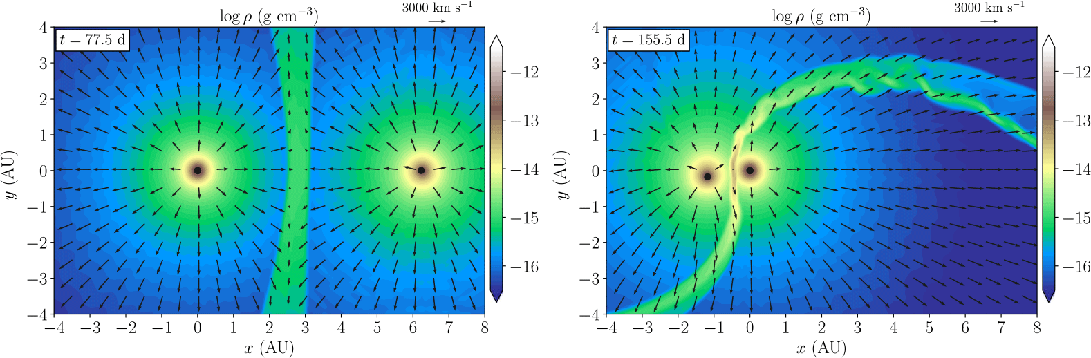
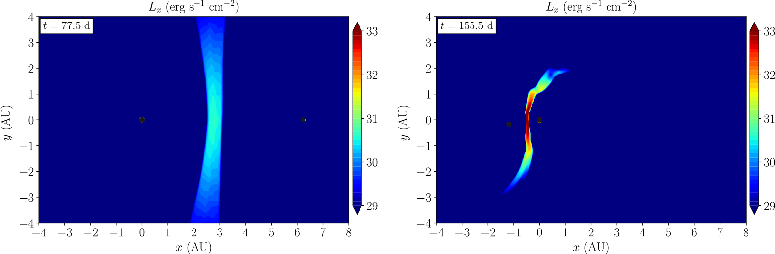
, and the winds of both stars are adiabatic which makes it unlikely to experience accretion close to periastron. Figure 1 and 2 show our simulations of Mk 34 close to periastron and apastron. The shape of the CWS changes between a conical shape and a spiral. Indeed the simulations show that there is no accretion at any point during the orbital period. To study these processes quantitatively, we conducted 3D hydrodynamical simulations of representative systems, focusing on colliding winds and their transition to accretion regimes. These simulations reveal how such interactions shape both the circumstellar medium and stellar evolution.
Simulations of the colliding wind binary Mk 34. Left: Density at apastron, showing a conical shell with a wide angle. Right: Density at periastron, showing a transition into a spiral. There is no accretion at any point during the orbital period, as the two stars have comparable wind momentum.

Figure 1 Long description
Panel A: A density plot at apastron. The x-axis ranges from -4 to 8 astronomical units (AU) and the y-axis ranges from -4 to 4 AU. The plot shows a conical shell with a wide angle, indicated by the color gradient and arrows representing wind direction. Panel B: A density plot at periastron. The x-axis ranges from -4 to 8 AU and the y-axis ranges from -4 to 4 AU. The plot shows a transition into a spiral pattern, with the color gradient and arrows indicating the wind direction and density changes.
Simulations of the colliding wind binary Mk 34. Left: X-ray emission at apastron. Right: X-ray emission at periastron. Color codes are in log scale.

2. Colliding winds with accretion
While Mk 34 exemplifies a system where colliding winds remain stable and accretion is suppressed, other binaries exhibit different behavior when the wind momentum ratio decreases. We extend our simulations to such systems to investigate how accretion can proceed against a stellar wind. Accretion against wind is rare and challenging to simulate. In this case the arriving gas experiences an opposing force by the wind and radiation of the secondary.
 $\eta$
Car was the first system where accretion against wind was suggested and tested (Soker Reference Soker2005; Kashi & Soker Reference Kashi and Soker2007; Kashi & Soker Reference Kashi and Soker2008; Kashi & Soker Reference Kashi and Soker2009; Kashi & Soker Reference Kashi and Soker2016). Hydrodynamical simulations by Akashi et al. (Reference Akashi, Kashi and Soker2013) found dense clumps formed by instabilities in the primary wind of
 $\eta$
Car, which then hit the secondary close to periastron passage. Kashi (Reference Kashi2017) and Kashi (Reference Kashi2019) showed that such filaments get accreted onto the secondary, and radiative braking or inhibition did not stop the accretion.
In Kashi et al. (Reference Kashi, Michaelis and Kaminetsky2022) we ran a numerical experiment of ejecting winds in a massive colliding wind binary system, and quantified the accretion onto the secondary star under different primary mass loss rates. The goal was to test accretion against wind problem and quantify the effect of the secondary wind in reducing the accretion rate below the classical Bondi-Hoyle-Lyttleton (BHL) value that assumes no wind from the secondary. We set a binary system comprising a LBV primary and a WR secondary, with
 $M_1 = 80 \, ~\rm{M_\odot}$
and
 $M_2 = 20 \, ~\rm{M_\odot}$
. For the fiducial run, the primary mass loss rate is
 $\dot{M}_1 = 3 \times 10^{-4} ~\rm{M_{\odot}}~\rm{yr^{-1}}$
with a wind terminal velocity value of
 $v_{1,\infty} = 500 ~\rm{km~s^{-1}}$
. The secondary mass loss rate is
 $\dot{M}_2 = 10^{-5} ~\rm{M_{\odot}}~\rm{yr^{-1}}$
, with a of
 $v_{2,\infty} = 3000 \, ~\rm{km~s^{-1}}$
and a momentum ratio
 $\eta = 0.2$
. By increasing the primary mass loss rate, we reduced the momentum ratio
 $\eta$
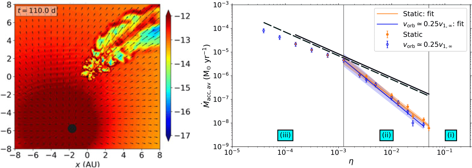
and checked the resulted accreted mass on the companion. The CWS exhibits strong instabilities, forming dense clumps and filaments. The secondary gravity pulls these filaments, leading to accretion. The secondary wind attempts to flow against the incoming gas, forming bubbles. Figure 3 shows an example for an extreme case where the secondary wind is almost extinguished by the wind of the primary. Figure 3 (right panel) shows the accretion rates. For
 $\eta\gt0.05$
there was no accretion (region (i) in Figure 3). For smaller values accretion occurs while the wind of the secondary is still dominant, and we get sub-BHL accretion (region (ii)). The instabilities in the CWS form clumps that have a velocity component in the direction of the flow but also have the acceleration of the secondary. Depending on the parameters, some of the clumps can be pulled towards the secondary and get accreted. As long as the wind of the secondary is able to push part of the clumps away and prevent them from being accreted, the accretion follows a power law of about
 $\dot{M}_{\rm acc} \propto \eta^{-1.73}$
for static stars and steeper
 $\dot{M}_{\rm acc} \propto \eta^{-1.86}$
when orbital motion is included. For very low
 $\eta$
the secondary wind almost does not exist. Accretion under such conditions (region (iii) in Figure 3) is directly onto the secondary as there is not colliding wind structure, but instead a geometry that resembles BHL accretion.
Left: A simulation with a
 $80~\rm{M_\odot}$
primary and
 $20~\rm{M_\odot}$
secondary on a circular orbit of
 $a=6~\rm{AU}$
. The momentum ratio of the two winds is almost as low as the threshold where the secondary wind is shut. This situation is representative for a giant eruption with a relatively low mass loss or a secondary with a strong wind of its own. Behind the secondary (marked by the small black circle at the center of the grid) a turbulent wind is formed. In such a case the accretion is sub-BHL and the accretion rate is highly fluctuating. An accretion disk is not formed under these conditions as there is insufficient angular momentum. Right: Time averaged accretion rates results from simulations of accretion at different secondary to primary wind momentum ratios (
 $\eta$
). Region (i) – No accretion: For
 $0.05 \lt \eta$
the secondary wind pushes away all the primary wind material so there is a well-defined colliding wind structure with a conical shape and no accretion. Region (ii) – Sub-BHL Accretion: For
 $0.01 \lt \eta \lt 0.05$
there is a transition region, in which accretion is very sporadic, mass can occasionally be accreted but for most of the time the secondary wind and radiation prevent accretion. For
 $0.001 \lt \eta \lt 0.01$
accretion occurs most of the time. The accretion rate and the accretion duty cycle are larger as
 $\eta$
decreases. The accretion rate satisfies a power-law relation with a slope of
 $\sim -1.8$
. Region (iii) – BHL accretion: For
 $\eta \lesssim 0.001$
the accretion becomes continuous in time and the accretion rate is close to BHL. The two most left points are results of new simulations with extremely low
 $\eta$
, indicative of a secondary with almost no wind at all.

3. The effect of accretion on the accreted star
Accretion at very high rates can lower the effective temperature of a star and thereby weaken its wind, as proposed by Kashi & Soker (Reference Kashi and Soker2009) for accretion near periastron in
 $\eta$
Car, and later confirmed in simulations (Kashi Reference Kashi2017). Kashi et al. (Reference Kashi, Davidson and Humphreys2016) modeled state changes triggered by a giant eruption using energy-conserving approaches and found that the star developed a wind with velocities of a few
 $\times 100~\rm{km~s^{-1}}$
and an initial mass-loss rate of
 $\sim 0.1~\rm{M_{\odot}~yr^{-1}}$
, which declined over time. The outflow, powered by
 $\kappa$
-mechanism radial pulsations, persisted for about 200 years, comparable to the recovery timescale of
 $\eta$
Car after its giant eruption.
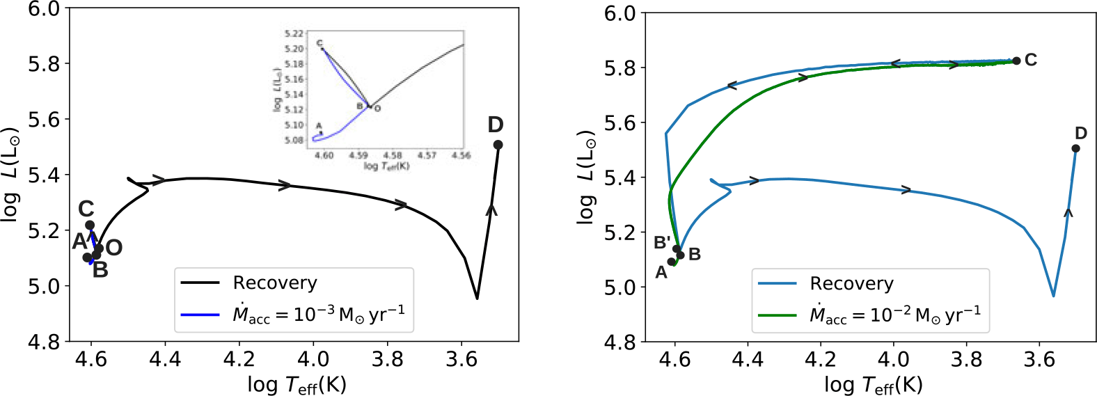
In Mukhija & Kashi (Reference Mukhija and Kashi2024) we examined the response of a massive companion star in a binary system to rapid gas accretion during a Giant Eruption of the primary. The accretion rate is governed by the erupting star’s mass loss, the binary separation, and the radiation field of the accretor, which can reduce the inflowing material. To isolate the stellar response, we adopted a simplified setup with a constant accretion rate, tracking how accumulated material alters the outer layers and surface parameters. Using the 1D stellar evolution code mesa, we modeled the evolution of a
 $30~\rm M_{\odot}$
star. The reference case followed its track from the ZAMS to the end of helium burning without accretion (Figure 4). From point B, we introduced accretion over 20 yrs with different rates. High accretion (
 $\gtrsim 10^{-2}-10^{-1}~\rm M_{\odot}~yr^{-1}$
) led to cooling, while lower rates kept the star on the hotter side of the HR diagram.
Stellar evolutionary tracks for a
 $30~\rm M_{\odot}$
star under different accretion rates were computed using mesa. Left panel: For an accretion rate of
 $10^{-3}~\rm M_{\odot}~yr^{-1}$
, the segment from B to C represents the accretion phase, while C-O and O-D mark the recovery. In this scenario, the C-O portion corresponds to the loss of gravitational energy through stellar winds, producing a vertical luminosity drop at low accretion rates. This drop occurs because high temperatures at point C drive wind-induced mass loss. Right panel: For a higher accretion rate of
 $10^{-2}~\rm M_{\odot} yr^{-1}$
, the star undergoes flashes during accretion. After accretion ends, the star shifts to the hot side of the HR diagram and continues evolving. Here, B-C again denotes the accretion phase, while the recovery is represented by the segments C-B’ and B’-D.

At high rates flashes appeared during accretion, and once accretion ended, the star moved to the hot side of the HR diagram and continued evolving. For low rates, the higher surface temperature triggered wind-driven mass loss shortly after accretion, lowering luminosity. Early in the accretion phase, both luminosity and effective temperature rose rapidly as gravitational energy from infalling gas was converted into thermal energy in the outer layers. As evolution proceeded, L and R stabilized, while
 $T_{\rm eff}$
declined under high accretion due to the dominance of outer layers. High accretion rates also induced significant compression in the outer envelope, producing fluctuations in luminosity during the first days of the accretion episode.
Mass ejection obscures the system, and only after the material dissipates (on timescales of decades to centuries) can the system be fully revealed. Both stars undergo changes during the eruption, but variations in high-excitation lines along the orbit may indicate whether the secondary remained hot or experienced cooling. However, because the ejection timescale is comparable to the recovery time from accretion, the secondary may already have returned to a hotter state by the time it becomes observable.
4. Accretion in a B[e]SG systems
GG Car (HD 94878) is a binary B[e] supergiant (B[e]SG) system that has been investigated for half a century (e.g., Kraus et al. Reference Kraus, Oksala and Nickeler2013; Porter et al. Reference Porter, Grant, Blundell and Lee2021; Porter et al. Reference Porter, Blundell and Lee2022). The primary a mass is
 $M_1 = 24 \pm 4 ~\rm{M_\odot}$
, and highly luminous with
 $\log(L_1/\rm{L_\odot}) = 5.26 \pm 0.19$
, and the secondary mass is taken to be
 $M_2 = 7.2 ~\rm{M_\odot}$
. (Porter et al. Reference Porter, Grant, Blundell and Lee2021). Earlier work on the evolutionary history of GG Car generally assumed that both stars evolved in a manner similar to isolated single stars (Kraus et al. Reference Kraus, Oksala and Nickeler2013; Kraus Reference Kraus2019). Porter et al. (Reference Porter, Grant, Blundell and Lee2021) advanced a different interpretation, treating GG Car as an interacting binary.
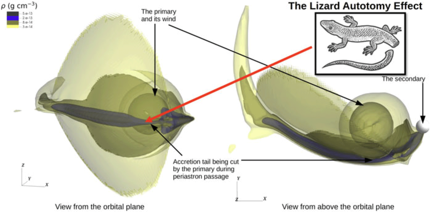
In Kashi (Reference Kashi2023) we simulated the hydrodynamics of the wind flow of GG Car and obtained the mass accretion rate onto the secondary and the observed lightcurve. We found that the accretion takes a geometric form that resembles inhomogeneous BHL accretion. The primary wind flows from both sides of the secondary and focused by its gravity into a curved tail. Part of the accretion tail flows towards the secondary and gets accreted, and part of it flows outwards and creates a spiral structure. Accretion also takes place from other directions but at a lower rate. After periastron passage a clear dense accretion disk is obtained around the secondary. We identified an effect related to the orbital motion of the two stars, wherein the accretion tail is severed by the primary star – the Lizard Autotomy Effect (Figure 5). As part of this effect, the primary star re-accretes wind that it had previously ejected. The Lizard Autotomy Effect results in an outwardly expanding spiral shell composed of broken segments. We suggested that such tails exists in other B[e]SGs systems and can be the source of the circumstellar material observed in such systems. The accretion onto the secondary also forms a disk around the secondary (not a circumbinary disk) near periastron that later disperses. Some of the gas later remains, and form dense filament. The formation of such a disk can be accompanied by the launching of two opposite jets perpendicular to the plane of the disk. These two jets can push ambient gas and form a bipolar structure, like those observed around some B[e]SGs (Torres et al. Reference Torres, Cidale and Kraus2018; Liimets et al. Reference Liimets, Kraus and Moiseev2022).
A 3D view of the GG Car binary system close to periastron passage. There is a dense tail behind the secondary, part of which is an accretion tail towards the secondary and part is outflowing away from it. The secondary takes a sharp elliptical turn close to periastron and as a result the close primary and its wind cut the tail and creates a gap in the tail – the Lizard Autotomy Effect. The process repeats every periastron passage, creating an outflowing spiral with gaps.

5. Conclusions
We investigated a complex physical system consisting of two massive stars in a binary configuration, which may follow eccentric orbits. Each star launches a powerful stellar wind, and the interaction between them gives rise to a shocked region where the winds collide, producing hot plasma that emits in the X-ray range. Our results span three representative regimes: (1) stable colliding winds without accretion (Mk 34), (2) systems exhibiting sub-BHL accretion near periastron (
 $\eta$
Car-like configurations), and (3) persistent disk-mediated accretion in B[e] supergiants (GG Car). Together, these cases delineate the transition from colliding-wind dominance to accretion dominance across massive binaries.
In cases where one star possesses a weaker wind momentum it can accrete material from the stronger wind of the primary. This accretion may be continuous, intermittent, or restricted to specific orbital phases, most notably near periastron when the stars are closest and the density and velocity gradients are strongest. The onset of accretion often disrupts the colliding wind structure, either partially or entirely, thereby altering or suppressing the X-ray emission generated in the shocked region. The accreted material might form a circumstellar structure around the secondary, such as an accretion disk or a more transient accretion belt. The presence of such a disk has multiple consequences: it can obscure or absorb part of the ionizing radiation emitted by the secondary, thereby modifying the ionization state of the circumstellar environment and affecting the production of high-ionization emission lines across the system. Furthermore, the accumulated material changes the photospheric boundary conditions of the accreting star, increasing its luminosity and potentially altering its evolutionary path.
The author thanks the organizers for this very interesting symposium. We acknowledge the Ariel HPC Center at Ariel University for providing computing resources that have contributed to the research results reported within this paper.
 80 M⊙
 20 M⊙
 a=6 AU
 η
 0.05<η
 0.01<η<0.05
 0.001<η<0.01
 η
 ∼−1.8
 η≲0.001
 η
 30 M⊙
 10−3 M⊙ yr−1
 10−2 M⊙yr−1

 Open access

