1. Introduction
Transport of mass, momentum, energy, charge and other physical quantities are of tremendous significance to scientists and engineers. In the literature, such transport processes have been described mathematically using microtransport equations, which are continuum equations applicable at length scales much larger than molecular length scales. For example, the ion conservation equations employed in describing electroosmotic processes are microtransport equations (Probstein Reference Probstein1994). The Navier–Stokes equation is a micro-continuum equation that describes the transport of momentum during flow for a relatively simple class of fluid materials – Newtonian fluids (Leal Reference Leal2007). Most engineering applications however involve macroscale processes, which occur over length scales much larger than those for which microtransport equations are derived. Thus, while microtransport equations may still be used to describe these macrotransport processes, the disparity in length scales in the two situations is challenging to surmount numerically even with present day computers. Particle-level microtransport equation-based approaches (Guazzelli & Morris Reference Guazzelli and Morris2011) such as Stokesian dynamics (Brady & Bossis Reference Brady and Bossis1988; Sierou & Brady Reference Sierou and Brady2001), the force coupling method (Sune & Maxey Reference Sune and Maxey2003; Yeo & Maxey Reference Yeo and Maxey2011) and the boundary element method (Pozrikidis Reference Pozrikidis1992; Ingber et al. Reference Ingber, Feng, Graham and Brenner2008) have improved our understanding of such various suspension properties as viscosity, first and second normal stress differences, and particle migration behaviour, and their dependencies on particle size and volume fraction. But these techniques are computationally demanding due to the need of incorporating far-field as well as near-field hydrodynamic interactions for multiple particles at the same time (Brady & Bossis Reference Brady and Bossis1988; Sierou & Brady Reference Sierou and Brady2001), and have traditionally been limited to simple, periodic domains containing a relatively small number of particles. While the number of particles in a box in Stokesian dynamics simulations has steadily increased over the past three decades, with the most recent version capable of handling hundreds of thousands of particles (Fiore & Swan Reference Fiore and Swan2019), it is still computationally expensive and cannot handle the flow of concentrated suspensions through complex geometries over length scales of practical interest.
One way to solve this computational challenge is to derive macrotransport equations by averaging microtransport equations over length scales larger than those relevant to the microscale processes, but smaller than those pertinent to the macroscale process. Several models have been introduced over the past two decades to obtain a macrotransport description of the migration of particles in flowing suspensions (Jenkins & McTigue Reference Jenkins and McTigue1990; Drew & Lahey Reference Drew and Lahey1993; Nott & Brady Reference Nott and Brady1994; Jackson Reference Jackson1997; Morris & Boulay Reference Morris and Boulay1999; Fang et al. Reference Fang, Mammoli, Brady, Ingber, Mondy and Graham2002; Guazzelli & Morris Reference Guazzelli and Morris2011; Lecampion & Garagash Reference Lecampion and Garagash2014; Municchi, Nagrani & Christov Reference Municchi, Nagrani and Christov2019), and one of the more prominent ones among these has been the suspension balance model (Nott & Brady Reference Nott and Brady1994; Morris & Boulay Reference Morris and Boulay1999; Fang et al. Reference Fang, Mammoli, Brady, Ingber, Mondy and Graham2002; Guazzelli & Morris Reference Guazzelli and Morris2011). This macrotransport model introduces an additional level of coarsening by volume averaging the continuity and momentum equations, first for the suspension as a whole, and then only for the particulate phase. The averaged equations are then closed by assuming that non-zero gradients in the particulate normal stresses result in a difference in the average particulate and suspension velocities. Averaging the microtransport equations also produces new, lumped, physical parameters. For instance, in a dilute suspension of spheres subjected to simple shear flow, a volume averaging of the stresses reveals that such a suspension may be modelled as Newtonian fluid to leading order in the volume fraction of spheres, with a viscosity equal to the Einstein viscosity (Einstein Reference Einstein1906; Batchelor Reference Batchelor1970; Kim & Karrila Reference Kim and Karrila2005; Leal Reference Leal2007; Guazzelli & Morris Reference Guazzelli and Morris2011). The new variable that results from the averaging process in the derivation of the suspension balance model is a shear-induced migration flux, which exhibits a scaling of  $\dot {\gamma }^{\prime }a^{\prime 2},$
 $\dot {\gamma }^{\prime }$ being the local shear rate and
 $a^{\prime }$ being the particle radius, and is a monotonically increasing function of the particle volume fraction
 $\phi$. When the complete non-Newtonian rheology of the suspension is included in the framework of the suspension balance model, it successfully describes the fully developed particle distributions in various flow geometries (Morris & Boulay Reference Morris and Boulay1999; Fang et al. Reference Fang, Mammoli, Brady, Ingber, Mondy and Graham2002; Ramachandran & Leighton Reference Ramachandran and Leighton2008; Boyer, Pouliquen & Guazzelli Reference Boyer, Pouliquen and Guazzelli2011b), and the agreement is nearly quantitative even in such complicated flows as resuspension in a settling tube (Ramachandran & Leighton Reference Ramachandran and Leighton2007a,Reference Ramachandran and Leightonb). The suspension balance model thus makes a tremendous simplification in the modelling of suspension flows and particle migration by coarsening the physics from the level of particles to the length scale corresponding to the characteristic dimension of the flow (typically the smaller length scale in the cross-section of the flow conduit). We note here that advancements to the suspension balance approach have been presented in the literature in recent years, with the inclusion of the frictional rheology (Boyer, Guazzelli & Pouliquen Reference Boyer, Guazzelli and Pouliquen2011a) to model viscoplastic suspension stresses at volume fractions approaching maximum packing (Lecampion & Garagash Reference Lecampion and Garagash2014). In this work we have chosen to focus on the suspension balance approach we have adopted previously (Ramachandran & Leighton Reference Ramachandran and Leighton2008; Ramachandran Reference Ramachandran2013), recognizing that the generated results will be restricted to volume fractions below 50 % (Zarraga, Hill & Leighton Reference Zarraga, Hill and Leighton2000).
Despite the advantages of the suspension balance model, three-dimensional simulations for the flow of concentrated suspensions through complicated geometries based on the model are computationally challenging (Lam et al. Reference Lam, Chen, Tam and Yu2003; Miller & Morris Reference Miller and Morris2006; Ramachandran & Leighton Reference Ramachandran and Leighton2007b), as singularities are observed in regions where the shear stresses vanish (e.g. at the centreline in the tube flow of suspensions). A practical example of such a geometry is the Hele-Shaw geometry or the pressure-driven flow between two parallel plates, which is encountered in applications such as powder injection moulding (Lam et al. Reference Lam, Chen, Tam and Yu2003), proppant transport (Hormozi & Frigaard Reference Hormozi and Frigaard2017; Dontsov et al. Reference Dontsov, Boronin, Osiptsov and Derbyshev2019) or in the testing of the spreading properties of cement grout in rock fractures (Shamu et al. Reference Shamu, Zou, Kotzé, Wiklund and Håkansson2020). In the Hele-Shaw geometry, the shear stresses vanish at the centreplane between the two Hele-Shaw plates to leading order, and this can lead to complexities in the numerical solution of the suspension balance model. Additionally, the largest dimensions in the flow geometry may significantly exceed the characteristic cross-sectional dimension – the channel depth. Thus, a macrotransport equation that further reduces the dimensionality of the problem can be extremely helpful to simulate the particle, velocity and pressure distributions for length scales encountered in engineering processes.
The objective of this paper is to derive a depth-averaged macrotransport equation describing the hydrodynamic transport of a concentrated suspension of rigid, non-colloidal, neutrally buoyant particles flowing through a Hele-Shaw geometry. Inspiration for this paper may be traced back to the work of Taylor (Reference Taylor1953), who obtained a macrotransport equation describing the axial spreading of a bolus of solute in the flow of a Newtonian fluid through a tube. The partial differential equation (PDE) describing the motion of the cross-section-averaged concentration  $\overline {c^{\prime }}$, with the axial spreading being termed as Taylor dispersion, becomes
 \begin{equation} \frac{\partial{\overline{c^{\prime }}}}{\partial t^{\prime }}+U^{\prime }\frac{\partial{\overline{c^{\prime }}}}{\partial x^{\prime }}=D_{{eff}^{\prime }}\frac{\partial^{2}{\overline{c^{\prime }}}}{\partial x^{\prime ^{2}}}. \end{equation}
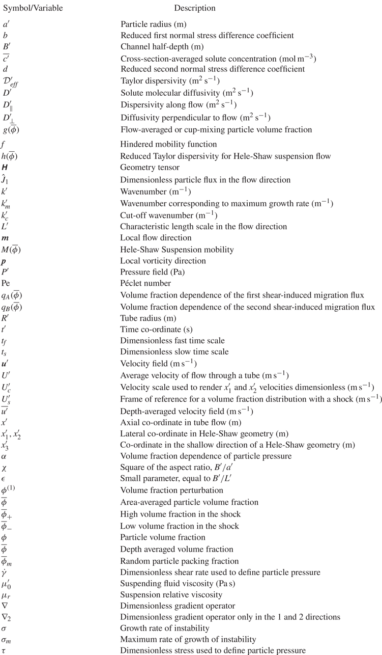
Note that throughout the manuscript, dimensional variables will be denoted using the prime symbol (see Table 2 in Appendix A for a complete list of symbols). In the above equation,  $x^{\prime }$ is the axial co-ordinate,
 $t^{\prime }$ represents time,
 $U^{\prime }$ is the volume-averaged flow velocity through the tube and
 $D_{eff}^{\prime }$ is the Taylor dispersion coefficient, which is defined as
 \begin{equation} D_{eff}^{\prime }=\frac{1}{48} \frac{{U^{\prime }}^{2}R^{\prime 2}}{D^{\prime }}=\frac{Pe^{2}D^{\prime }}{48},\quad \text{where} \ Pe=\frac{U^{\prime }R^{\prime }}{D^{\prime }}. \end{equation}
Here,  $R^{\prime }$ is the radius of the tube and
 $D^{\prime }$ represents the molecular diffusivity of the solute. According to the above PDE, when a solute slug is introduced, the centre of mass of the solute moves at the average fluid velocity
 ${U^{\prime }}$ while simultaneously spreading out in a diffusive manner in the flow direction owing to Taylor dispersion. The above expression for
 $D_{eff}^{\prime }$ is valid when the Péclet number is much larger than unity. More recently, it was shown that analogous equations describe the flow of a concentrated suspension through a tube (Griffiths & Stone Reference Griffiths and Stone2012; Ramachandran Reference Ramachandran2013), and the flow of a dense granular suspension along an incline (Christov & Stone Reference Christov and Stone2014). For example, from the work of Ramachandran (Reference Ramachandran2013), the cross-section averaged, one-dimensional macrotransport equation for a concentrated suspension of rigid, neutrally buoyant, non-colloidal spheres for non-dilute suspensions flowing through a tube is
 \begin{equation} \frac{\partial{\bar{\phi}}}{\partial t^{\prime }}+U^{\prime }\frac{\textrm{d}g}{\textrm{d}{\bar{\phi}}}\frac{\partial{\bar{\phi}}}{\partial x^{\prime }}=\frac{\partial}{\partial x^{\prime }} \left(\frac{R^{\prime 3}U^{\prime }}{a^{\prime 2}}h(\bar{\phi})\frac{\partial{\bar{\phi}}}{\partial x^{\prime }}\right). \end{equation}
Here,  $\bar {\phi }$ is the area-averaged particle volume fraction,
 $a^{\prime }$ is the radius of the spherical particle,
 $g(\bar {\phi })$ is the dimensionless, flow-averaged particle volume fraction (Ramachandran & Leighton Reference Ramachandran and Leighton2007a) (
 $g=\iint u^{\prime }\phi \, \textrm {d}A^{\prime } / \iint u^{\prime }\, \textrm {d}A^{\prime }$, where
 $u^{\prime }$ and
 $\phi$ are the axial velocity and volume fraction profiles, respectively, in the tube cross-section) and
 $h(\bar {\phi })$
 $R^{\prime 3}U^{\prime }/a^{\prime 2}$ is the Taylor dispersion coefficient. The above equation was derived from the suspension balance model of Nott & Brady (Reference Nott and Brady1994) coupled with the constitutive equations of Zarraga et al. (Reference Zarraga, Hill and Leighton2000), by performing a multiple time scale expansion (Pagitsas, Nadim & Brenner Reference Pagitsas, Nadim and Brenner1986; Hinch Reference Hinch1991) involving the small parameter
 $\epsilon = R^{\prime 3}/(a^{\prime 2}L^{\prime })$, where
 $L^{\prime }$ is the characteristic length scale of the geometry along the flow direction.
In this paper we extend the treatment of Ramachandran (Reference Ramachandran2013) to the flow of a suspension in a Hele-Shaw geometry. While depth-averaged models are available in the literature for suspension flows (e.g. see Dontsov & Peirce Reference Dontsov and Peirce2014; Hormozi & Frigaard Reference Hormozi and Frigaard2017; Wong, Lindstrom & Bertozzi Reference Wong, Lindstrom and Bertozzi2019; Dontsov et al. Reference Dontsov, Boronin, Osiptsov and Derbyshev2019), we formally derive, for the first time, a macrotransport equation that includes a Taylor dispersion term along with contributions from shear-induced migration and fluxes arising due to gradients in the local geometry of the flow. We also perform a linear stability analysis on the resulting macrotransport equation for the classic viscous miscible fingering problem (Wooding Reference Wooding1962; Tan & Homsy Reference Tan and Homsy1986) as applied to suspension flows. We have structured this paper as follows. Section 2 describes the governing equations for the particle and velocity distributions, based on the suspension balance model coupled with constitutive equations. In § 3 a two-time-scale perturbation expansion is implemented to arrive at the final form of the macrotransport equation. In § 4 we discuss the physical significance of each term in the equation. We show that a negative step change in volume fraction along the flow direction relaxes continuously; however, a positive step change in volume fraction leads to the emergence of viscous miscible fingering effects. Section 5 then implements a linear stability analysis of the viscous miscible fingering problem for a concentrated suspension flowing through Hele-Shaw geometry using a quasi-steady state approximation (QSSA) and ends with results. Section 6 presents conclusions and future work recommendations. The manuscript is written in a way so as to afford the reader two possible ways to read the article. The first (and obvious) option is to read the manuscript in its entirety. However, readers exclusively interested in understanding the various terms in the macrotransport equation, the nature of the instability and its implications for the evolution of the particle distribution, may skip §§ 2 and 3 and proceed directly on to §§ 4 and 6.
2. Theoretical model
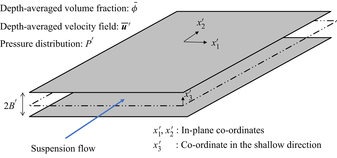
Consider a concentrated suspension of rigid, non-colloidal, neutrally buoyant spheres flowing between two parallel, stationary plates under the influence of a pressure field  $P^{\prime }$ (see figure 1). The suspending medium is Newtonian with a viscosity
 $\mu _0^{\prime }$. The Hele-Shaw geometry has a thickness of
 $2B^{\prime }$ in the depth direction (3), and a characteristic length scale of
 $L^{\prime }$ in the lateral directions, 1 and 2. Here
 $x_1^{\prime }$ and
 $x_2^{\prime }$ are the co-ordinates along the lateral directions, while
 $x_3^{\prime }$ is the co-ordinate in the depth direction, along which the equations and variables will be averaged. We denote the depth-averaged volume fraction by
 $\bar{\phi}$ and the depth-averaged velocity field by
 $\bar{{u_{i}}}^{\prime }$. Following the development of the suspension balance model in our previous work (Ramachandran & Leighton Reference Ramachandran and Leighton2008), and using
 $L^{\prime }$ as the length scale for the
 $x_1^{\prime }$ and
 $x_2^{\prime }$ directions,
 $B^{\prime }$ as the length scale for the
 $x_3^{\prime }$ direction,
 $U_c^{\prime }$ as the velocity scale and
 $\mu _0^{\prime } U_c^{\prime } L^{\prime }/B^{\prime 2}$ as the stress scale, the following dimensionless governing equations emerge:
 \begin{gather} \boldsymbol{\nabla}_{2_j}u_j+\frac{\partial u_3}{\partial x_3}=0,\end{gather}
 $$\begin{gather} \epsilon^2\boldsymbol{\nabla}_{2_j}\left[\mu_r\left(\boldsymbol{\nabla}_{2_j}u_i+\boldsymbol{\nabla}_{2_i}u_j\right)\right]+\epsilon^2\frac{\partial}{\partial x_3}\left(\mu_r\frac{\partial u_3}{\partial x_i}\right)+\frac{\partial}{\partial x_3}\left(\mu_r\frac{\partial u_i}{\partial x_3}\right)\nonumber\\ \hspace{-11pc}=\frac{\partial P}{\partial x_i}+\epsilon\boldsymbol{\nabla}_{2_j}\left(\alpha\tau {\mathsf{H}}_{ij}\right), \end{gather}$$
 \begin{gather} \epsilon^4\boldsymbol{\nabla}_{2_j}\left[\mu_r\left(\frac{\partial u_3}{\partial x_j}+\mu_r\frac{\partial u_j}{\partial x_3}\right)\right] +\epsilon^2\frac{\partial}{\partial x_3}\left(2\mu_r\frac{\partial u_3}{\partial x_3}\right)=\frac{\partial P}{\partial x_3}+\epsilon\frac{\partial }{\partial x_3}\left(\alpha\tau\right), \end{gather}
 \begin{gather} \chi \epsilon \left[\frac{\partial \phi}{\partial t}+\boldsymbol{\nabla}_{2_j}\left(u_j\phi\right)+\frac{\partial}{\partial x_3} \left(u_3\phi\right)\right] =\frac{2}{9}\,\epsilon^2\boldsymbol{\nabla}_{2_i}\left[f\boldsymbol{\nabla}_{2_j}\left(\alpha\tau {\mathsf{H}}_{ij}\right)\right] +\frac{2}{9}\,\frac{\partial}{\partial x_3}\left[f\frac{\partial }{\partial x_3}\left(\alpha\tau \right) \right]. \end{gather}
Equation (2.1a) is the continuity equation, (2.1b) represents the momentum equations in the lateral directions  $(x_1\text { and } x_2)$, (2.1c) is the momentum equation in the shallow direction
 $(x_3)$ and (2.1d) is the particle conservation equation. Here, the fields
 $P$,
 $u_i$ and
 $\phi$ are the dimensionless pressure, velocity and volume fraction, respectively. The operator
 $\boldsymbol {\nabla }_2$ is the gradient operator defined in the 1–2 co-ordinates only. The subscripted indices
 $i$ and
 $j$ assume values of 1 and 2 only. The parameter
 $\epsilon$ is the aspect ratio,
 \begin{equation} \epsilon=\frac{B^{\prime }}{L^{\prime }}, \end{equation}
and is the small parameter that will be exploited in the asymptotic expansion to follow. The quantity  $\alpha$ in (2.1) is the reduced normal stress (Zarraga et al. Reference Zarraga, Hill and Leighton2000), given by
 \begin{equation} \alpha(\phi)=2.17\phi^3\textrm{e}^{2.34\phi}\left(1-\frac{\phi}{\phi_m}\right)^{-0.01}. \end{equation}
By allowing the reduced normal stress to diverge at maximum packing fraction, we overcome the issue of singularity in the volume fraction at  $x_3=0$ (e.g. see Miller & Morris Reference Miller and Morris2006; Ramachandran & Leighton Reference Ramachandran and Leighton2007b, Reference Ramachandran and Leighton2008). The results presented in this paper are relatively insensitive to values of the exponent less than
 $0.01$. In (2.1),
 $\tau$ is a local measure of the dimensionless shear stress (Ramachandran & Leighton Reference Ramachandran and Leighton2008), given by
 \begin{equation} \tau=\mu_r(\phi)\dot{\gamma}, \end{equation}
where the shear rate  $\dot {\gamma }$ is defined as
 \begin{align} \dot{\gamma}=\sqrt{\epsilon^2\left(\boldsymbol{\nabla}_{2_j}u_i+\boldsymbol{\nabla}_{2_i}u_j\right)\boldsymbol{\nabla}_{2_j}u_i+\epsilon^4\left(\boldsymbol{\nabla}_{2_j}u_3+\frac{\partial u_j}{\partial x_3}\right)\boldsymbol{\nabla}_{2_j}u_3+ \left(\frac{\partial u_i}{\partial x_3}\right)^2+\epsilon^2\frac{\partial u_i}{\partial x_3}\boldsymbol{\nabla}_{2_i}u_3}. \end{align}
In (2.1),  ${\mathsf{H}}_{ij}$ is the geometry tensor, defined as
 \begin{equation} {\mathsf{H}}_{ij}=\delta_{ij}-b\frac{m_im_j}{m_km_k}+d\frac{p_ip_j}{p_kp_k}, \end{equation}
where  $m_i$ and
 $p_i$, which are the velocity and vorticity directions, are given by
 \begin{equation} m_i=u_i \quad \mathrm{and} \quad p_i=\epsilon_{ij3}m_j. \end{equation}
Schematic of the flow geometry.

The boundary conditions for the velocity component in the depth direction,  $u_3$, are
 \begin{equation} \left.u_3\right|_{x_3=0,1}=0, \end{equation}
due to the antisymmetry about the centerplane and the zero normal flow condition at the wall. The boundary conditions for  $u_i$ are the symmetry of the in-plane components of the velocity field at the midplane,
 \begin{equation} \left.\frac{\partial u_i}{\partial x_3}\right|_{x_3=0}=0, \end{equation}
and the no-slip boundary condition at the wall,
 \begin{equation} \left.u_i\right|_{x_3=1}=0. \end{equation}
The boundary conditions for the particle concentration are the no-flux restriction at the wall, and symmetry at the midplane, i.e.
 \begin{equation} \left.\left[\chi \epsilon u_3\phi-\frac{2}{9}\,f(\phi)\frac{\partial }{\partial x_3}\left(\alpha\tau H_{33}\right)\right]\right|_{x_3=0,1}=0. \end{equation}
Equation (2.8) allows us to simplify the above equation to
 \begin{equation} \left.\left[\frac{2}{9}\,f(\phi)\frac{\partial }{\partial x_3}\left(\alpha\tau\right)\right]\right|_{x_3=0,1}. \end{equation}
3. Multiple time scale expansion
We follow the procedure in Ramachandran (Reference Ramachandran2013) and implement a multiple time scale expansion of the governing equations and boundary conditions (Pagitsas et al. Reference Pagitsas, Nadim and Brenner1986; Hinch Reference Hinch1991). To begin, we need to define a small parameter relevant to this problem. For this, consider the ratio of time scale for shear-induced migration over the depth and the convective time scale in the flow direction,
 \begin{equation} \frac{B^{\prime 2}/\left[(U_c^{\prime }/B^{\prime })a^{\prime 2}\right]}{L^{\prime }/U_c^{\prime }}=\chi \epsilon. \end{equation}
Here, the parameter  $\chi$ is
 \begin{equation} \chi=\frac{B^{\prime 2}}{a^{\prime 2}}. \end{equation}
In the Taylor dispersion limit (Brenner & Edwards Reference Brenner and Edwards1993; Probstein Reference Probstein1994; Ramachandran Reference Ramachandran2013),  $\chi \epsilon =B^{\prime 3}/a^{\prime 2}L^{\prime }$ is a small parameter, i.e. the length scale
 $L^{\prime }$ in the direction parallel to the Hele-Shaw plates needs to be significantly greater than the induction length scale
 $B^{\prime 3}/a^{\prime 2}$ (Chapman Reference Chapman1990; Nott & Brady Reference Nott and Brady1994; Hampton et al. Reference Hampton, Mammoli, Graham and Tetlow1997; Ramachandran & Leighton Reference Ramachandran and Leighton2007a; Lecampion & Garagash Reference Lecampion and Garagash2014).
In dimensionless terms the two time variables for the multiple time scale expansion are  $t_f=t$ (the fast time scale) and
 $t_s=\chi \epsilon t$ (the slow time scale). The partial derivative
 $\partial /\partial t$ is thus transformed to
 \begin{equation} \partial/\partial t = \partial/\partial t_f+\chi \epsilon\partial/\partial t_s. \end{equation}
After implementing this transformation, the only governing equation in (2.1) that is modified is the particle balance equation (2.1d), and it becomes
 $$\begin{align} &\chi
\epsilon \left[\frac{\partial \phi}{\partial t_f}+\chi
\epsilon\frac{\partial \phi}{\partial
t_s}+\boldsymbol{\nabla}_{2_j}\left(u_j\phi\right)+\frac{\partial}{\partial
x_3} \left(u_3\phi\right)\right] \notag\\
&\quad =\frac{2}{9}\,\epsilon^2\boldsymbol{\nabla}_{2_i}\left[f\boldsymbol{\nabla}_{2_j}\left(\alpha\tau
{\mathsf{H}}_{ij}\right)\right]
+\frac{2}{9}\,\frac{\partial}{\partial
x_3}\left[f\frac{\partial }{\partial x_3}\left(\alpha\tau
\right) \right].
\end{align}$$
All the dependent variables in the problem are now functions of five independent variables:  $t_f$,
 $t_s$,
 $x_1$,
 $x_2$ and
 $x_3$.
The dependent variables can now be written as the following regular perturbation expansions in the small parameter  $\chi \epsilon$:
 \begin{equation} \left. \begin{gathered} \phi=\phi^{(0)}+(\chi \epsilon) \phi^{(1)}+(\chi \epsilon)^2\phi^{(2)}+ \cdots, \\ P=P^{(0)}+(\chi \epsilon) P^{(1)}+(\chi \epsilon)^2P^{(2)}+ \cdots,\\ u_i=u_i^{(0)}+(\chi \epsilon) u_i^{(1)}+(\chi \epsilon)^2u_i^{(2)}+ \cdots\,, \\ u_3=u_3^{(0)}+(\chi \epsilon) u_3^{(1)}+(\chi \epsilon)^2u_3^{(2)}+ \cdots. \end{gathered} \right\} \end{equation}
In the subsections that follow, we will implement the multiple time scale expansion procedure. As a note, the overline that will appear over several variables henceforth represents the operator for performing an average over the depth of the Hele-Shaw geometry, i.e.
 \begin{equation} \bar{\mathcal{F}}\left(x_1,x_2,t\right)=\int_0^1\mathcal{F}\left(x_1,x_2,x_3,t\right)\,\textrm{d}x_3. \end{equation}
Also, the expansion procedure produces a host of functions:  $M$,
 $F$,
 $g$,
 $G$ and
 $Q_1$ through
 $Q_{12}$. These functions are summarized in Appendix B.
To conclude this subsection, we note that the depth averages of the volume fraction and the two-dimensional velocity field are given by the averages of their zeroth-order approximations, i.e.
 \begin{equation} \bar{\phi}=\overline{\phi^{(0)}} \quad \text{and}\quad \overline{u_i}=\overline{u_i^{(0)}}, \end{equation}
implying that
 \begin{equation} \overline{\phi^{(j)}}=0 \quad \text{and} \quad \overline{u_i^{(j)}}=0, \end{equation}
for  $j\geq 1$.
3.1. The  $O[(\chi \epsilon )^0]$ problem

To leading order in  $\chi \epsilon$, the particle balance equation (3.4) is
 \begin{equation} \frac{2}{9}\,\frac{\partial}{\partial x_3}\left[f(\phi^{(0)})\frac{\partial }{\partial x_3}\left(\alpha\tau\right)^{(0)} \right]=0. \end{equation}
The no-flux boundary condition (2.12) at the walls at this order,
 \begin{equation} \left.\left[\frac{2}{9}\,f(\phi^{(0)})\frac{\partial }{\partial x_3}\left(\alpha\tau\right)^{(0)}\right]\right|_{x_3=0,1}, \end{equation}
combined with (3.9) yields the following expression for the particle pressure:
 \begin{equation} \left(\alpha\tau\right)^{(0)}=c'. \end{equation}
Here  $c'$ is the constant of integration. To obtain the stress
 $\tau ^{(0)}$ required for computing the volume fraction profile, the continuity and momentum equations in (2.1a) to (2.1c) are examined at
 $O[(\chi \epsilon )^0]$ to yield
 \begin{gather} \boldsymbol{\nabla}_{2_j}u_j^{(0)}+\frac{\partial u_3^{(0)}}{\partial x_3}=0, \end{gather}
 \begin{gather} \frac{\partial}{\partial x_3}\left[\mu_r(\phi^{(0)})\frac{\partial u_i^{(0)}}{\partial x_3}\right]=\boldsymbol{\nabla}_{2_j} P^{(0)}, \end{gather}
 \begin{gather} \frac{\partial P^{(0)}}{\partial x_3}=0. \end{gather}
As the pressure is invariant in the  $x_3$ direction at this order, (3.12b) can be integrated with respect to
 $x_3$. Doing this once yields
 \begin{equation} \mu_r(\phi^{(0)})\frac{\partial u_i^{(0)}}{\partial x_3}=\boldsymbol{\nabla}_{2_j} P^{(0)}x_3, \end{equation}
where the symmetry condition (2.9) has been applied. The stress,  $\tau$, at this order, defined using (2.4) and (2.5), can be deduced from the above result as
 \begin{equation} \tau^{(0)}=\left|{\boldsymbol{\boldsymbol{\nabla}}}_2 P^{(0)}\right|x_3. \end{equation}
Note that  $\left |{\boldsymbol {\boldsymbol {\nabla }}}_2 P^{(0)}\right |$ is independent of
 $x_3$ due to (3.12c). Substitution of the above result in (3.11) yields
 \begin{equation} \alpha(\phi^{(0)})x_3=\alpha_w, \end{equation}
where  $\alpha _w$ is the reduced normal stress evaluated at the wall. The above equation provides the volume fraction distribution for a given depth-averaged volume fraction
 $\bar {\phi }$,
 \begin{equation} \phi^{(0)}(\bar{\phi},x_3)=\alpha^{{-}1}\left[\frac{\alpha_w}{x_3}\right], \end{equation}
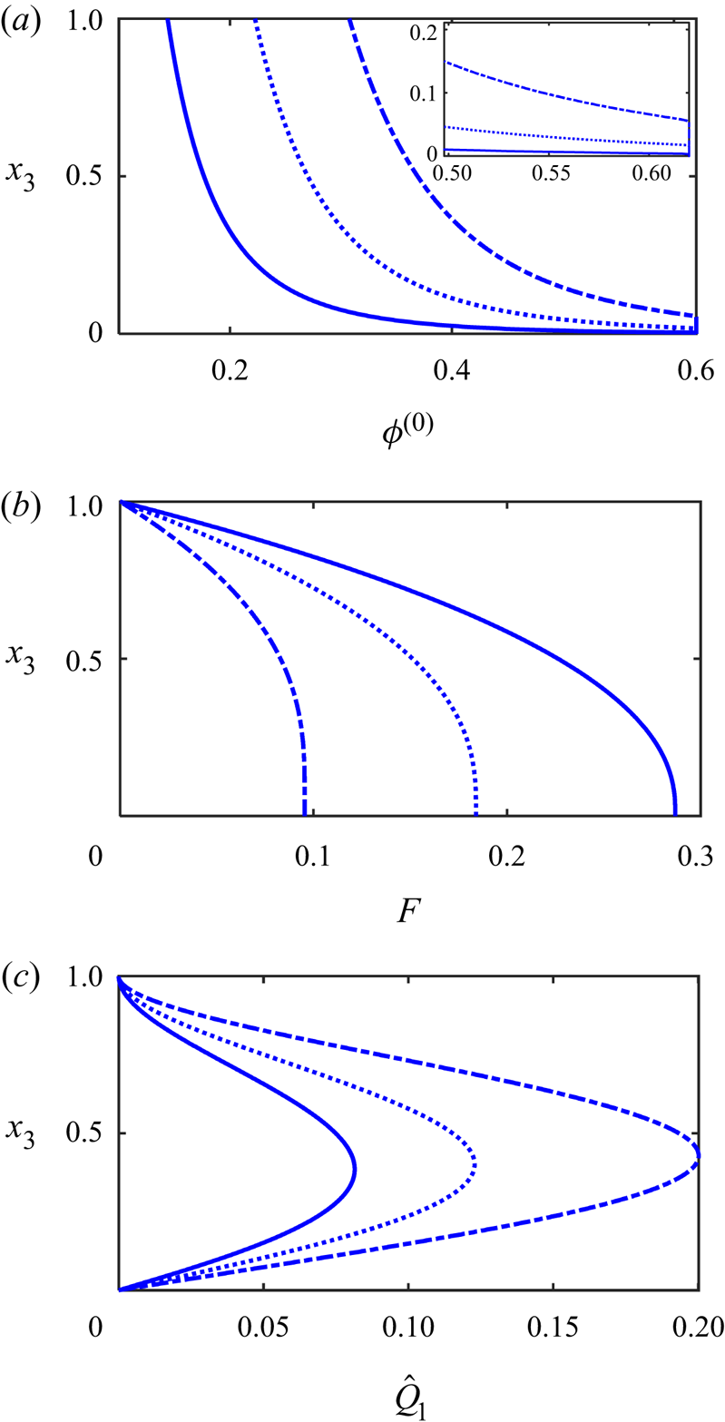
In figure 2(a) we have shown the volume fraction profile over the depth for different  $\bar {\phi }$. Similar to tube flow of suspensions (Phillips et al. Reference Phillips, Armstrong, Brown, Graham and Abbott1992; Hampton et al. Reference Hampton, Mammoli, Graham and Tetlow1997; Fang et al. Reference Fang, Mammoli, Brady, Ingber, Mondy and Graham2002; Miller & Morris Reference Miller and Morris2006; Ramachandran & Leighton Reference Ramachandran and Leighton2008; Ramachandran Reference Ramachandran2013), there is a region of maximum packing fraction around the centreline due to the phenomenon of shear-induced migration (Koh, Hookham & Leal Reference Koh, Hookham and Leal1994; Lyon & Leal Reference Lyon and Leal1998; Fang et al. Reference Fang, Mammoli, Brady, Ingber, Mondy and Graham2002; Gao & Gilchrist Reference Gao and Gilchrist2008; Lecampion & Garagash Reference Lecampion and Garagash2014; Yadav, Reddy & Singh Reference Yadav, Reddy and Singh2016; Dontsov et al. Reference Dontsov, Boronin, Osiptsov and Derbyshev2019), which becomes thicker as the volume fraction increases.
Predictions of the zeroth-order profiles of (a) volume fraction ( $\phi ^{(0)}$, (3.16)), (b) the function quantifying the in-plane velocity (
 $F$, (3.17)) and (c) the velocity along the thin direction (
 $\hat {Q}_1=Q_1//M$, (3.26)), as functions of the co-ordinate in the thin direction,
 $x_3$. The solid, dotted and dash–dotted curves are the results for depth-averaged volume fractions of 20 %, 30 % and 45 %. The inset in subfigure (a) provides a zoomed-in view of the volume fraction profiles near the centreline.

To get the velocity distribution, (3.13) may be divided by  $\mu _r(\phi ^{(0)})$ and integrated in
 $x_3$ to produce the following expression for
 $u_i$ after the application of the no-slip boundary condition (2.10):
 \begin{equation} u_i^{(0)}={-}F(\bar{\phi},x_3)\boldsymbol{\nabla}_{2_i} P^{(0)}. \end{equation}
Here, the function  $F$ is defined as
 \begin{equation} F(\bar{\phi},x_3)=\int_{x_3}^1\frac{\xi \,\textrm{d}\xi}{\mu_r[\phi^{(0)}(\bar{\phi},\xi)]}. \end{equation}
The velocity distribution is shown as a function of  $x_3$ for different depth-averaged volume fractions in figure 2(b). Again, analogous to tube flow, the maximum packing region near the centreline leads to blunting of the velocity profile due to the high viscosity associated with this region (Koh et al. Reference Koh, Hookham and Leal1994; Lyon & Leal Reference Lyon and Leal1998; Fang et al. Reference Fang, Mammoli, Brady, Ingber, Mondy and Graham2002; Gao & Gilchrist Reference Gao and Gilchrist2008; Lecampion & Garagash Reference Lecampion and Garagash2014; Yadav et al. Reference Yadav, Reddy and Singh2016; Dontsov et al. Reference Dontsov, Boronin, Osiptsov and Derbyshev2019). As
 $\bar {\phi }$ increases, the average velocity for a given pressure gradient decreases, and the size of the blunted zone increases. Notably, the sizes of the maximum packing regions and the blunted zones are smaller than the corresponding ones for tube flow. This is because the area of a region of a given width near the centre represents a smaller fraction of the total area for tube Poiseuille flow than plane Poiseuille flow.
The depth-averaged velocity at this order is
 \begin{equation} \overline{u_i^{(0)}}=\overline{u_i}={-}M(\bar{\phi})\boldsymbol{\nabla}_{2_i} P^{(0)}. \end{equation}
Here, the function  $M$ quantifies the mobility of the suspension, and is defined as
 \begin{equation} M(\bar{\phi})=\int_0^1 F(\bar{\phi},x_3)\,\textrm{d}x_3. \end{equation}
Integrating the continuity equation (3.12a), and applying the boundary conditions for  $u_3$ (see (2.8)), we get the governing equation for the pressure distribution at this order,
 \begin{equation} \boldsymbol{\nabla}_{2_j}[M(\bar{\phi})\boldsymbol{\nabla}_{2_j} P^{(0)}]=0. \end{equation}
Finally, we derive an expression for  $u_3^{(0)}$, which will be required in the
 $O(\chi \epsilon )$ analysis. Using the continuity equation (3.12a), we get
 \begin{equation} \frac{\partial u_3^{(0)}}{\partial x_3}=\boldsymbol{\nabla}_{2_j} [F(\bar{\phi},x_3)\boldsymbol {\nabla}_{2_j} P^{(0)}]. \end{equation}
Integrating the above equation with respect to  $x_3$, we get
 \begin{equation} u_3^{(0)}=\boldsymbol{\nabla}_{2_j} [Q_1(\bar{\phi},x_3) \boldsymbol{\nabla}_{2_j} P^{(0)}], \end{equation}
where
 \begin{equation} Q_1(\bar{\phi},x_3)=\int_0^{x_3}F(\bar{\phi},\xi)\,\textrm{d}\xi. \end{equation}
Using the following modified version of the averaged continuity equation (3.21),
 \begin{equation} \boldsymbol{\nabla}_2^2 P^{(0)}={-}\frac{M^{\prime }(\bar{\phi})}{M(\bar{\phi})}\boldsymbol{\nabla}_{2_j}\bar{\phi}\boldsymbol{\nabla}_{2_j} P^{(0)}, \end{equation}
and the relationship between  $\overline {u_j}$ and
 $\boldsymbol {\nabla }_2 P^{(0)}$ in (3.19), (3.23) can be simplified to
 \begin{equation} u_3^{(0)}=\hat{Q}_1(\bar{\phi},x_3)\boldsymbol{\nabla}_{2_j}\bar{\phi} \quad \overline{u_j}, \end{equation}
where
 \begin{equation} \hat{Q}_1(\bar{\phi},x_3)=\frac{M^{\prime }(\bar{\phi})}{M^2(\bar{\phi})}Q_1(\bar{\phi},x_3)-\frac{1}{M(\bar{\phi})}\frac{\partial Q_1}{\partial \bar{\phi}}(\bar{\phi},x_3). \end{equation}
Shown in figure 2(c) is the function  $\hat {Q}_1$ as a function of
 $x_3$ for different
 $\bar {\phi }$. For positive gradients in the volume fraction along the flow direction
 $\left (\boldsymbol {\nabla }_{2_j}\bar {\phi }\ \overline {u_j}>0\right )$, the suspension viscosity increases in the flow direction, and this increase is stronger near the centreplane of the Hele-Shaw geometry than the walls. As a result, there is a decrease in the planar velocity field
 $u_i^{(0)}$ in the flow direction, which, by conservation of mass, leads to an expulsion of suspension from the centreplane to the walls, i.e. a positive
 $u_3^{(0)}$. Similarly, negative gradients in the volume fraction
 $(\boldsymbol {\nabla }_{2_j}\bar {\phi }\ \overline {u_j}<0)$ along the flow direction lead to negative
 $u_3^{(0)}$.
3.2. The $O[(\chi \epsilon )^1]$ problem

The particle balance equation (3.4) at  $O[(\chi \epsilon )^1]$ is
 $$\begin{align}
&\frac{\partial \phi^{(0)}}{\partial
t_f}-\nabla_{2_j}\left[F\left(\overline{\phi},x_3\right)\phi^{(0)}\left(\overline{\phi},x_3\right)\nabla_{2_j}
P^{(0)}\right]\notag\\ &\quad+ \frac{\partial}{\partial x_3}
\left[u_3^{(0)}\phi^{(0)}\left(\overline{\phi},x_3\right)\right]=\frac{2}{9}\frac{\partial}{\partial
x_3}\left[f\left(\phi\right)\frac{\partial }{\partial
x_3}\left(\alpha\tau \right)
\right]^{(1)}.\end{align}$$
In the above equation, we have substituted the expression for  $u_i^{(0)}$ from (3.17). Integrating the above equation with respect to
 $x_3$ from 0 to 1, we get
 \begin{equation}
\frac{\partial \bar{\phi}}{\partial
t_f}-\boldsymbol{\nabla}_{2_j}
[G(\bar{\phi}) \boldsymbol{\nabla}_{2_j}
P^{(0)}]=0,
\end{equation}
where
 \begin{equation}
G(\bar{\phi})=\int_0^1F(\bar{\phi},\xi)\phi^{(0)}(\bar{\phi},\xi)\,\textrm{d}\xi.
\end{equation}
In (3.29) we have applied the no-flux boundary condition in (2.12) at this order, and also used the result for the zeroth-order particle pressure from (3.11). Using the following result from the chain rule,
 \begin{equation} \frac{\partial \phi^{(0)}}{\partial t_f}=\frac{\partial \phi^{(0)}}{\partial \bar{\phi}}\frac{\partial \bar{\phi}}{\partial t_f}, \end{equation}
we can manipulate (3.28) and (3.29) to arrive at
 $$\begin{align} &\frac{\partial
\phi^{(0)}}{\partial
\overline{\phi}}\nabla_{2_j}\left[G\left(\overline{\phi}\right)\nabla_{2_j}
P^{(0)}\right]-\nabla_{2_j}\left[F\left(\overline{\phi},x_{3}\right)\nabla_{2_j}
P^{(0)}\phi^{(0)}\right]\notag\\ &\quad +\frac{\partial}{\partial x_{3}}
\left(u_{3}^{(0)}\phi^{(0)}\right)=\frac{2}{9}\frac{\partial}{\partial
x_3}\left[f\left(\phi^{(0)}\right)\frac{\partial }{\partial
x_3}\left(\alpha\tau \right)^{(1)} \right].
\end{align}$$
To arrive at the right-hand side of the above equation from (3.28), we have used the constancy of  $(\alpha \tau )^{(0)}$ over the depth (3.11). After the integration of the above equation in
 $x_3$ and the implementation of the algebraic steps discussed in Appendix C, we get the volume fraction perturbation
 $\phi ^{(1)}$ as
 \begin{equation}
\phi^{(1)}
=Q_7(\bar{\phi},x_3)\frac{\boldsymbol{\nabla}_{2_j}\bar{\phi}
(-\boldsymbol{\nabla}_{2_j}
P^{(0)})}{|{\boldsymbol{\boldsymbol{\nabla}}}_{2}P^{(0)}|}=Q_7(\bar{\phi},x_3)\left(\frac{\boldsymbol{\nabla}_{2_j}\bar{\phi}\hspace{0.1in}\overline{u_j}}{\left|\overline{\boldsymbol{u}}\right|}\right).
\end{equation}
Note that  $\phi ^{(1)}$ is proportional to the directional derivative of
 $\bar {\phi }$ along the depth-averaged velocity vector.
To derive the velocity perturbation, we begin with (2.1b) at  $O[(\chi \epsilon )^1]$, which gives
 \begin{equation} \frac{\partial}{\partial x_3}\left(\mu_r\frac{\partial u_i}{\partial x_3}\right)^{(1)}=\boldsymbol{\nabla}_{2_i} P^{(1)}. \end{equation}
Integration of the above equation, followed by the application of the boundary condition at the wall and some simplifications (see Appendix D for details), yields
 \begin{equation} u_i^{(1)}=Q_{10}(\bar{\phi},x_3)\frac{\boldsymbol{\nabla}_{2_j}\bar{\phi}\boldsymbol{\nabla}_{2_j} P^{(0)}}{\left|\boldsymbol{\boldsymbol{\nabla}}_{2} P^{(0)}\right|}\boldsymbol{\nabla}_{2_i} P^{(0)}=\frac{Q_{10}(\bar{\phi},x_3)}{M(\bar{\phi})}\left(\frac{\boldsymbol{\nabla}_{2_j}\bar{\phi}\hspace{0.1in}\overline{u_j}}{\left|\overline{\boldsymbol{u}}\right|}\right)\overline{u_i}. \end{equation}
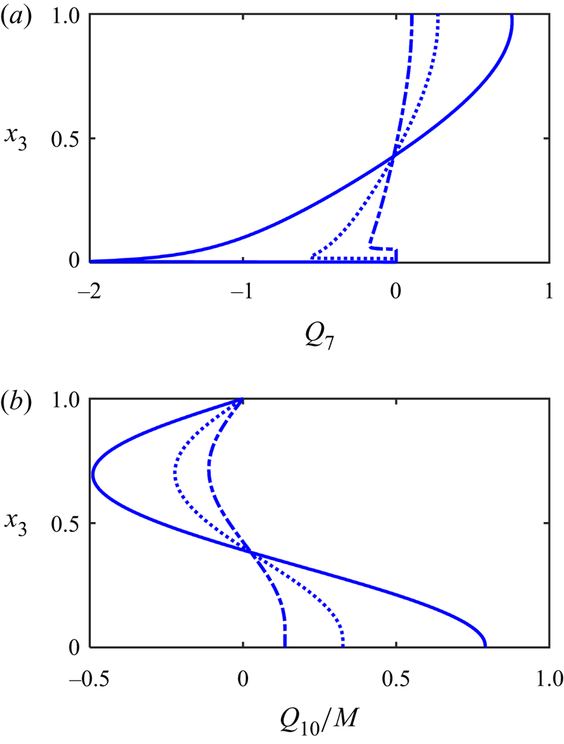
In figure 3 we have shown the functions  $Q_7$ and
 $Q_{10}/M$ corresponding to the volume fraction and velocity distributions at
 $O\left (\chi \epsilon \right )$ for
 $\bar {\phi }=0.2, 0.3$ and 0.45. When
 $\boldsymbol {\nabla }_{2_j}\bar {\phi }\ \overline {u_j}>0$, the volume fraction perturbation is negative near the centre (see figure 3a). As explained in Ramachandran (Reference Ramachandran2013), this is due to two reasons: the displacement of a low volume fraction suspension into a region of high volume fraction, and the positive
 $u_3^{(0)}$ velocity which drives particles away from the centre and towards the walls when
 $\left (\boldsymbol {\nabla }_{2_j}\bar {\phi }\ \overline {u_j}>0\right )$. The greater the volume fraction, the smaller the perturbation due to the smaller contrast in the volume fraction between the centre and wall, and the weaker the magnitude of
 $u_3^{(0)}$. The negative value of
 $\phi ^{(1)}$ near the centre leads to a decrease in suspension viscosity there and, hence, a positive perturbation in the first-order velocity field (see figure 3b), the effect being stronger for higher volume fractions. Similar arguments can be used to deduce trends when
 $\boldsymbol {\nabla }_{2_j}\bar {\phi }\ \overline {u_j}<0$.
Predictions of the first-order profiles of (a) volume fraction ( $Q_7$, (3.33)) and (b) the function quantifying the in-plane velocity, (
 $Q_{10}/M$, (3.35)), as functions of the co-ordinate in the thin direction,
 $x_3$. The solid, dotted and dash–dotted curves are the results for depth-averaged volume fractions of 20 %, 30 % and 45 %.

We end this subsection by commenting that it is possible to determine the pressure  $P^{(1)}$ and the velocity component
 $u_3^{(1)}$ by employing the continuity equation, but these variables are not required to derive the macrotransport equation to be presented at the end of this section. Hence, the calculations of
 $P^{(1)}$ and
 $u_3^{(1)}$ will not be pursued.
3.3. The $O[(\chi \epsilon )^2]$ problem and the averaged equations

The particle balance equation (3.4) at  $O[(\chi \epsilon )^2]$ is
 $$\begin{align}
&\frac{\partial \phi^{(1)}}{\partial
t_f}+\boldsymbol{\nabla}_{2_i}\left(u_i^{(0)}\phi^{(1)}+u_i^{(1)}\phi^{(0)}\right)+\frac{\partial}{\partial
x_3} \left(u_3\phi\right)^{(1)}+\frac{\partial
\phi^{(0)}}{\partial t_s}\nonumber\\
&\quad =\frac{\epsilon^2}{(\chi\epsilon)^2}\frac{2}{9}\,\boldsymbol{\nabla}_{2_i}\left[f\boldsymbol{\nabla}_{2_j}\left(\alpha\tau
{\mathsf{H}}_{ij}\right)\right]^{(0)}
+\frac{2}{9}\,\frac{\partial}{\partial
x_3}\left[f\frac{\partial }{\partial x_3}\left(\alpha\tau
\right) \right]^{(2)}.
\end{align}$$
Note that we have preserved the leading order shear-induced migration term,  $({2}/{9})\epsilon ^2\boldsymbol {\nabla }_{2_i}[f\boldsymbol {\nabla }_{2_j}(\alpha \tau {\mathsf{H}}_{ij})]^{(0)}$, even though it is of order
 $\chi ^{-2}$ relative to other terms at this order. As will become clear later, the key particle flux that emerges from the left-hand side of the equation, the Taylor dispersion flux, does not have a component in the direction normal to the streamlines defined by the velocity field
 $\overline {u_i}$ (see (3.33) and (3.35)). The leading order source of particle flux perpendicular to the flow streamline is the shear-induced migration flux and, hence, it has to be retained.
We can use (3.14), (3.15) and (3.19) to write
 \begin{equation} (\alpha\tau {\mathsf{H}}_{ij})^{(0)}=\frac{\alpha_w(\bar{\phi})}{M(\bar{\phi})}\left|\overline{\boldsymbol{u}}\right| {\mathsf{H}}_{ij}^{(0)}, \end{equation}
where
 \begin{equation} {\mathsf{H}}_{ij}^{(0)}=\delta_{ij}-b\frac{\overline{u_i}\ \overline{u_j}}{\overline{u_k}\ \overline{u_k}}+d\frac{\epsilon_{ik3}\overline{u_k}\ \epsilon_{jl3}\overline{u_l}}{\overline{u_p}\ \overline{u_p}}. \end{equation}
This modifies (3.36) to
 \begin{equation} \frac{\partial \bar{\phi}}{\partial t_s}+\boldsymbol{\nabla}_{2_i}\left(\overline{u_i^{(0)}\phi^{(1)}}+\overline{u_i^{(1)}\phi^{(0)}}\right)=\boldsymbol{\nabla}_{2_i}\left[\frac{2}{9}\,\overline{f^{(0)}}\boldsymbol{\nabla}_{2_j}\left(\frac{\alpha_w(\bar{\phi})}{M(\bar{\phi})}\left|\overline{\boldsymbol{u}}\right| {\mathsf{H}}_{ij}^{(0)}\right)\right]. \end{equation}
Let us now consider the two convective terms on the left-hand side of the above equation. The first one, which arises due to the volume fraction perturbation  $\phi ^{(1)}$, can be written as
 \begin{equation} \overline{u_j^{(0)}\phi^{(1)}}={-}M(\bar{\phi})Q_{11}(\bar{\phi}) \left(\frac{\boldsymbol{\nabla}_{2_j}\bar{\phi}\ \overline{u_j}}{\left|\overline{\boldsymbol{u}}\right|}\right)\overline{u_i}, \end{equation}
where
 \begin{equation} Q_{11}(\bar{\phi})={-}\frac{1}{M(\bar{\phi})}\int_0^1F(\bar{\phi},\xi)Q_7(\bar{\phi},\xi)\,\textrm{d}\xi, \end{equation}
while the second one, which arises due to the perturbation,  $u_i^{(1)}$, in the velocity field, simplifies to
 \begin{equation} \overline{u_j^{(1)}\phi^{(0)}}=M(\bar{\phi})Q_{12}(\bar{\phi})\left(\frac{\boldsymbol{\nabla}_{2_j}\bar{\phi}\hspace{0.1in}\overline{u_j}}{\left|\overline{\boldsymbol{u}}\right|}\right), \end{equation}
with
 \begin{equation} Q_{12}(\bar{\phi})=\frac{1}{M(\bar{\phi})}\int_0^1Q_{10}(\bar{\phi},\xi)\phi^{(0)}(\bar{\phi},\xi)\,\textrm{d}\xi. \end{equation}
A negative sign has been added to the definition of  $Q_{11}$ in (3.41) to ensure that
 $Q_{11}$ is a positive function. Equation (3.39) thus becomes
 \begin{align}
\frac{\partial \bar{\phi}}{\partial
t_s}=\boldsymbol{\nabla}_{2_i}\left[M(\bar{\phi})h(\bar{\phi})\left(\frac{\boldsymbol{\nabla}_{2_j}\bar{\phi}\hspace{0.1in}\overline{u_j}}{\left|\overline{\boldsymbol{u}}\right|}\right)\overline{u_i}\right]+\frac{\epsilon^2}{(\chi\epsilon)^2}\boldsymbol{\nabla}_{2_i}\left[\frac{2}{9}\,\overline{f^{(0)}}\boldsymbol{\nabla}_{2_j}\left(\frac{\alpha_w(\bar{\phi})}{M(\bar{\phi})}\left|\overline{\boldsymbol{u}}\right|
{\mathsf{H}}_{ij}^{(0)}\right)\right],
\end{align}
where
 \begin{equation} h(\bar{\phi})=Q_{11}(\bar{\phi})-Q_{12}(\bar{\phi}). \end{equation}
After expanding out the shear-induced migration term in the above equation, we get
 $$\begin{align}
\frac{\partial \bar{\phi}}{\partial
t_s}&=\boldsymbol{\nabla}_{2_i}\left[h(\bar{\phi})\left(\frac{\boldsymbol{\nabla}_{2_j}\bar{\phi}\hspace{0.1in}\overline{u_j^{(0)}}}{\left|\overline{\boldsymbol{u}}\right|}\right)\overline{u_i}\right]+\frac{\epsilon^2}{(\chi\epsilon)^2}\boldsymbol{\nabla}_{2_i}
(q_A(\bar{\phi})\left|\overline{\boldsymbol{u}}\right|
{\mathsf{H}}_{ij}^{(0)}\boldsymbol{\nabla}_{2_j}\bar{\phi})\nonumber\\
&\quad +\frac{\epsilon^2}{(\chi\epsilon)^2}\boldsymbol{\nabla}_{2_i}\left[q_B(\bar{\phi})\boldsymbol{\nabla}_{2_j}\left(\left|\overline{\boldsymbol{u}}\right|
{\mathsf{H}}_{ij}^{(0)}\right)\right],
\end{align}$$
where
 \begin{equation} \left. \begin{gathered} q_A(\bar{\phi})=\frac{2}{9}\,\overline{f^{(0)}}\frac{\textrm{d}}{\textrm{d}\bar{\phi}}\left[\frac{\alpha_w(\bar{\phi})}{M(\bar{\phi})}\right],\\ q_B(\bar{\phi})=\frac{2}{9}\,\overline{f^{(0)}}\frac{\alpha_w(\bar{\phi})}{M(\bar{\phi})}. \end{gathered} \right\} \end{equation}
We now rewrite (3.29) with the pressure gradient  $\boldsymbol {\nabla }_{2_j}P^{(0)}$ replaced by the depth-averaged velocity field
 $\overline {u_i}$ using (3.19),
 \begin{equation} \frac{\partial \bar{\phi}}{\partial t_f}+\boldsymbol{\nabla}_{2_i}\left[g(\bar{\phi})\overline{u_i}\right]=0, \end{equation}
where the function  $g$ is the local flow-averaged volume fraction (Ramachandran & Leighton Reference Ramachandran and Leighton2007b; Ramachandran Reference Ramachandran2013), defined as
 \begin{equation} g(\bar{\phi})=\frac{G(\bar{\phi})}{M(\bar{\phi})}. \end{equation}
Multiplying (3.48) by  $\chi \epsilon$ and (3.46) by
 $\left (\chi \epsilon \right )^2$, and then summing the resulting equations, yields
 $$\begin{align}
\left(\chi\epsilon\right)\left[\frac{\partial
\bar{\phi}}{\partial
t}+\boldsymbol{\nabla}_{2_i}\left(g(\bar{\phi})\overline{u_i}\right)\right]
&=\left(\chi\epsilon\right)^2\boldsymbol{\nabla}_{2_i}\left[h(\bar{\phi})\left(\frac{\boldsymbol{\nabla}_{2_j}\bar{\phi}
u_j}{|\overline{\boldsymbol{u}}|}\right)\overline{u_i}\right]\nonumber\\
&\quad +\epsilon^2\boldsymbol{\nabla}_{2_i}(q_A(\bar{\phi})\left|\overline{\boldsymbol{u}}\right|
{\mathsf{H}}_{ij}^{(0)}\boldsymbol{\nabla}_{2_j}\bar{\phi})\notag\\
&\quad +\epsilon^2\boldsymbol{\nabla}_{2_i}
[q_B(\bar{\phi})\boldsymbol{\nabla}_{2_j}
(|\overline{\boldsymbol{u}}|
{\mathsf{H}}_{ij}^{(0)})].
\end{align}$$
Reverting to dimensional variables, we obtain
 $$\begin{align}
\frac{\partial \bar{\phi}}{\partial
t'}+\boldsymbol{\nabla}_{2_i}^{\prime
}[g(\bar{\phi})\overline{u'_i}] &=\frac{B^{\prime
3}}{a^{\prime 2}}\boldsymbol{\nabla}_{2_i}^{\prime
}\left[h(\bar{\phi})\left(\frac{\boldsymbol{\nabla}_{2_j}\bar{\phi}
\ \overline{u_j^{\prime
}}}{\left|\overline{\boldsymbol{u}}^{\prime
}\right|}\right)\overline{u_i^{\prime }}\right]\nonumber\\
&\quad +\frac{a^{\prime 2}}{B^{\prime
}}\boldsymbol{\nabla}_{2_i}^{\prime
}(q_A(\bar{\phi})|\overline{\boldsymbol{u^{\prime
}}}|
{\mathsf{H}}_{ij}^{(0)}\nabla^{\prime
}_{2_j}\bar{\phi})+\frac{a^{\prime 2}}{B^{\prime
}}\boldsymbol{\nabla}_{2_i}^{\prime
}[q_B(\bar{\phi})\boldsymbol{\nabla}_{2_j}^{\prime
}(|\overline{\boldsymbol{u}^{\prime }}|
{\mathsf{H}}_{ij}^{(0)})].
\end{align}$$
The above equation is the macrotransport equation for the depth-averaged volume fraction.
4. Discussion
The macrotransport equation governing the depth-averaged particle volume fraction,  $\bar {\phi }$, as derived in § 3, can be written as
 $$\begin{gather} \frac{\partial \bar{\phi}}{\partial t^{\prime }}+\underbrace{\boldsymbol{\nabla}_{2_i}^{\prime }[g(\bar{\phi})\overline{u_i^{\prime }}]}_{\text{Convection term}}=\underbrace{\boldsymbol{\nabla}_{2_i}^{\prime }\left[\mathcal{D}_{eff}^{\prime } \left(\frac{\overline{u_j^{\prime }}\boldsymbol{\nabla}_{2_j}^{\prime }\bar{\phi}}{\left|\overline{\boldsymbol{u}^{\prime }}\right|}\right)\frac{\overline{u_i^{\prime }}}{\left|\overline{\boldsymbol{u}^{\prime }}\right|}\right]}_{\text{Taylor dispersion term (TD)}}+\underbrace{\boldsymbol{\nabla}_{2_i}^{\prime }\left[q_{A}(\bar{\phi})\left(\frac{\left|\overline{\boldsymbol{u}^{\prime }}\right|a^{\prime 2}}{B^{\prime }}\right){\mathsf{H}}_{ij}\boldsymbol{\nabla}_{2_j}^{\prime }\bar{\phi}\right]}_{\text{First shear-induced migration term }(\text{SIM}_1)}\nonumber\\ +\underbrace{\boldsymbol{\nabla}_{2_i}^{\prime }\left\{q_B(\bar{\phi})\boldsymbol{\nabla}_{2_j}^{\prime }\left[\left(\frac{\left|\overline{\boldsymbol{u}^{\prime }}\right|a^{\prime 2}}{B^{\prime }}\right){\mathsf{H}}_{ij}\right]\right\}}_{\text{Second shear-induced migration term }(\text{SIM}_2)}. \end{gather}$$
Here,  $\overline {u_i^{\prime }}$ is the depth-averaged velocity field, given by
 \begin{equation} \overline{u_i^{\prime }}={-}\frac{B^{\prime 2}}{\mu_0^{\prime }}M(\bar{\phi}) \boldsymbol{\nabla}_{2_i}^{\prime }P^{\prime }, \end{equation}
 $\mathcal {D}_{eff}^{\prime }$ is the Taylor dispersivity,
 \begin{equation}
\mathcal{D}_{eff}^{\prime }=\frac{B^{\prime 3}}{a^{\prime
2}}|\overline{\boldsymbol{u}^{\prime
}}|h(\bar{\phi}),
\end{equation}
and depends on the magnitude of the depth-averaged velocity. The geometry tensor,  ${\mathsf{H}}_{ij}$, that appears in (4.1) has the definition,
 \begin{equation} {\mathsf{H}}_{ij}=\delta_{ij}-b\frac{\overline{u_i} \ \overline{u_j}}{\overline{u_k} \ \overline{u_k}}+ d\frac{\epsilon_{ik3}\overline{u_k} \ \epsilon_{jl3}\overline{u_l}}{\overline{u_p} \ \overline{u_p}}, \end{equation}
where  $b=-0.15$ and
 $d=-0.54$ are the reduced first and second normal stress difference coefficients (Zarraga et al. Reference Zarraga, Hill and Leighton2000). To determine the pressure distribution
 $P^{\prime }$ that is required to calculate the depth-averaged velocity field, we solve the continuity equation.
 \begin{equation} \boldsymbol{\nabla}_{2_i}^{\prime }[M(\bar{\phi})\boldsymbol{\nabla}_{2_i}^{\prime }P^{\prime }]=0. \end{equation}
The left-hand side of (4.1) involves the temporal term for  $\bar {\phi }$ and a convection term involving the two-dimensional, depth-averaged velocity field. On the right side, the first term is due to Taylor dispersion, and scales as
 $U_c^{\prime }B^{\prime 3}/a^{\prime 2}$, where
 $U_c^{\prime }$ is the characteristic velocity. As expected, the Taylor dispersion flux arises due to gradients in volume fraction only in the flow direction, indicated by the directional derivative of
 $\bar {\phi }$ along the local, depth-averaged velocity vector. We also have two shear-induced migration terms on the right-hand side of (4.1), SIM
 $_1$ and SIM
 $_2$ that each scale as
 $U_c^{\prime }a^{\prime 2}/B^{\prime }$. The SIM
 $_1$ flux arises due to gradients in the volume fraction while the SIM
 $_2$ flux arises due to gradients in the local shear rate
 $|\overline {\boldsymbol {u}^{\prime }}|/B^{\prime }$ and the local flow geometry
 $\boldsymbol{\mathsf{H}}$, the latter representing a measure of the curvature of streamlines corresponding to the depth-averaged velocity field.
The system of equations above relies on five functions that vary with the depth-averaged volume fraction, namely  $M(\bar {\phi })$,
 $g(\bar {\phi })$,
 $h(\bar {\phi })$,
 $q_A(\bar {\phi })$ and
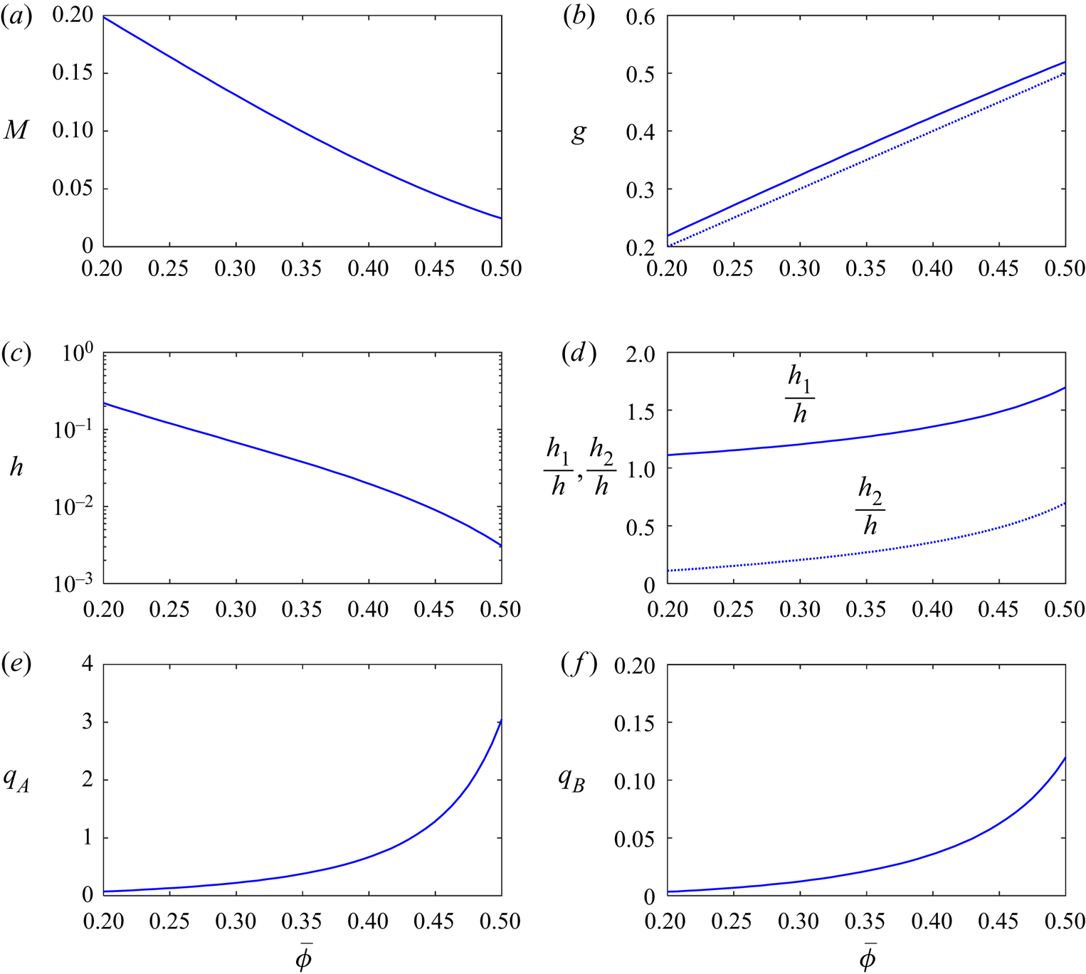
 $q_B(\bar {\phi })$. Figure 4 shows these functions for volume fractions in the range of
 $0.2\leq \bar {\phi }\leq 0.5$, over which the constitutive equations (Zarraga et al. Reference Zarraga, Hill and Leighton2000) used in the suspension balance equations are valid. The suspension mobility
 $M (\bar {\phi })$ connects the velocity with the pressure gradient (see (4.2)). Owing to the nonlinear relationship of viscosity and volume fraction (figure 4a),
 $M$ decreases monotonically with the volume fraction. Here
 $g (\bar {\phi })$ is the flow-averaged particle concentration at any given axial location. It is evident from figure 4(b) that for the volume fraction range of interest (20–50 %),
 $g(\bar {\phi })$ exceeds
 $\bar {\phi }$; this is due to the shear-induced migration of particles from the high shear stress, low velocity regions near the surfaces of the two Hele-Shaw plates to the low shear stress, high velocity regions near the Hele-Shaw centreplane (Phillips et al. Reference Phillips, Armstrong, Brown, Graham and Abbott1992; Hampton et al. Reference Hampton, Mammoli, Graham and Tetlow1997; Miller & Morris Reference Miller and Morris2006; Gao & Gilchrist Reference Gao and Gilchrist2008; Ramachandran & Leighton Reference Ramachandran and Leighton2008; Ramachandran Reference Ramachandran2013; Lecampion & Garagash Reference Lecampion and Garagash2014; Yadav et al. Reference Yadav, Reddy and Singh2016). The reduced Taylor dispersivity,
 $h (\bar {\phi })$, decreases monotonically with
 $\bar {\phi }$ (figure 4c). As shown in § 3 and also described in Ramachandran (Reference Ramachandran2013), it incorporates two contributions – one due to volume fraction perturbations about the zeroth-order volume fraction,
 $h_1=Q_{11}(\overline{\phi})$, and the other due to velocity perturbations about the zeroth-order velocity profile
 $h_2=Q_{12}(\overline{\phi})$ the latter arising due to changes in suspension viscosity. Note that
 $h_1$ is always larger than
 $h_2$, but
 $h_2$ contributes increasingly significantly to
 $h$ as
 $\bar {\phi }$ increases (see figure 4d). The functions
 $q_A (\bar {\phi })$ (figure 4e) and
 $q_B (\bar {\phi })$ (figure 4f) which are associated with the fluxes corresponding to SIM
 $_1$ and SIM
 $_2$, respectively, increase with
 $\bar {\phi }$, as expected, as shear-induced migration effects become stronger with particle volume fraction (Leighton & Acrivos Reference Leighton and Acrivos1987; Nott & Brady Reference Nott and Brady1994; Morris & Boulay Reference Morris and Boulay1999; Ramachandran & Leighton Reference Ramachandran and Leighton2008). The function,
 $q_B$, however, is typically an order of magnitude weaker than
 $q_A$; hence, variations in streamline curvature and shear rate are expected to have a weaker impact on the particle distribution than gradients in the volume fraction. The ratio of the SIM
 $_1$ flux to the Taylor dispersion flux is
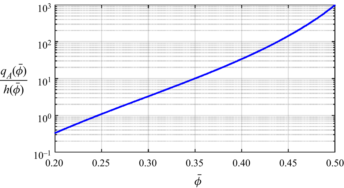
 $(a^{\prime 4}/B^{\prime 4})q_A(\bar {\phi })/h(\bar {\phi })$. As can be seen in figure 5, the largest value of this ratio in the range of volume fractions explored by us is approximately 1000 at
 $\bar {\phi }=0.5$. For aspect ratios
 $B^{\prime }/a^{\prime }>10$, which is true for most experiments avoiding finite particle size and wall slip effects for concentrated suspensions (Jana, Kapoor & Acrivos Reference Jana, Kapoor and Acrivos1995; Mills & Snabre Reference Mills and Snabre1995), the shear-induced migration flux is less than 10 % of the Taylor dispersion flux even for
 $\bar {\phi }=0.5$. But this is true only along the local velocity vector, as the particle flux due to the Taylor dispersion normal to the local flow direction is identically zero. Perpendicular to the local depth-averaged velocity field, only shear-induced migration (SIM1 and SIM2) can lead to a particle flux due to gradients in particle volume fraction, shear rate and streamline curvature.
The functions appearing in the macrotransport equation: (a) the suspension mobility,  $M (\bar {\phi })$ (3.20); (b) the flow-averaged volume fraction,
 $g (\bar {\phi })$ (3.49) (the dotted line is the parity line, equal to
 $\bar {\phi }$); (c) the reduced Taylor dispersivity,
 $h (\bar {\phi })$ (3.45); (d) the relative contributions of the volume fraction and velocity perturbations,
 $h_1 (\bar {\phi })$ (3.35) and
 $h_2 (\bar {\phi })$ (3.33), respectively, to the reduced Taylor dispersivity (note that
 $h=Q_{11}-Q_{12}$ (3.45)); (e) the prefactor of SIM
 $_1$,
 $q_A (\bar {\phi })$ (3.47); and (f) the prefactor of SIM
 $_2$,
 $q_B (\bar {\phi })$ (3.47).

The volume fraction dependence of the ratio of the shear-induced migration flux to the Taylor dispersion flux along the flow direction.

A few additional comments pertaining to the macrotransport equation (4.1) are in order here. First, due to the direct proportionality of the convection, Taylor dispersion and shear-induced migration terms to the velocity scale, the velocity dependence of these terms can be factored out and absorbed into the time derivative term, suggesting that the evolution of the particle volume fraction distribution is dependent only on an appropriately defined strain experienced by the suspension. Second, the macrotransport equation set (4.1)–(4.5) represents a coupled PDE system in  $\bar {\phi }$ and
 $P^{\prime }$, which can be conveniently fed to commercially available solvers such as COMSOL® to determine these variables as functions of
 $t^{\prime }$ and
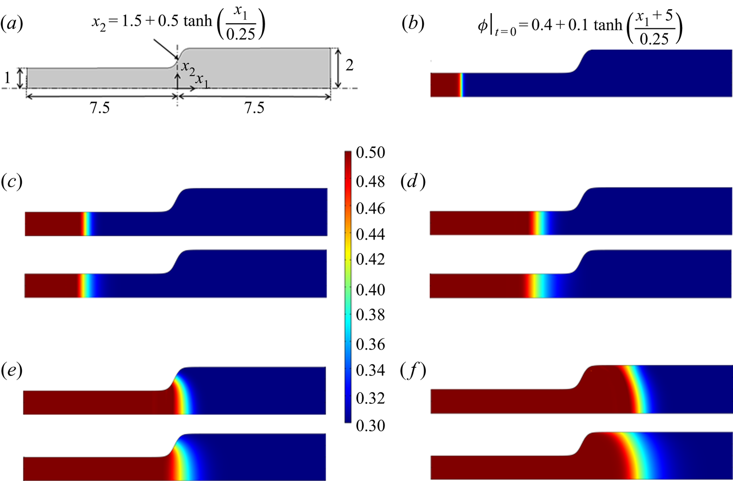
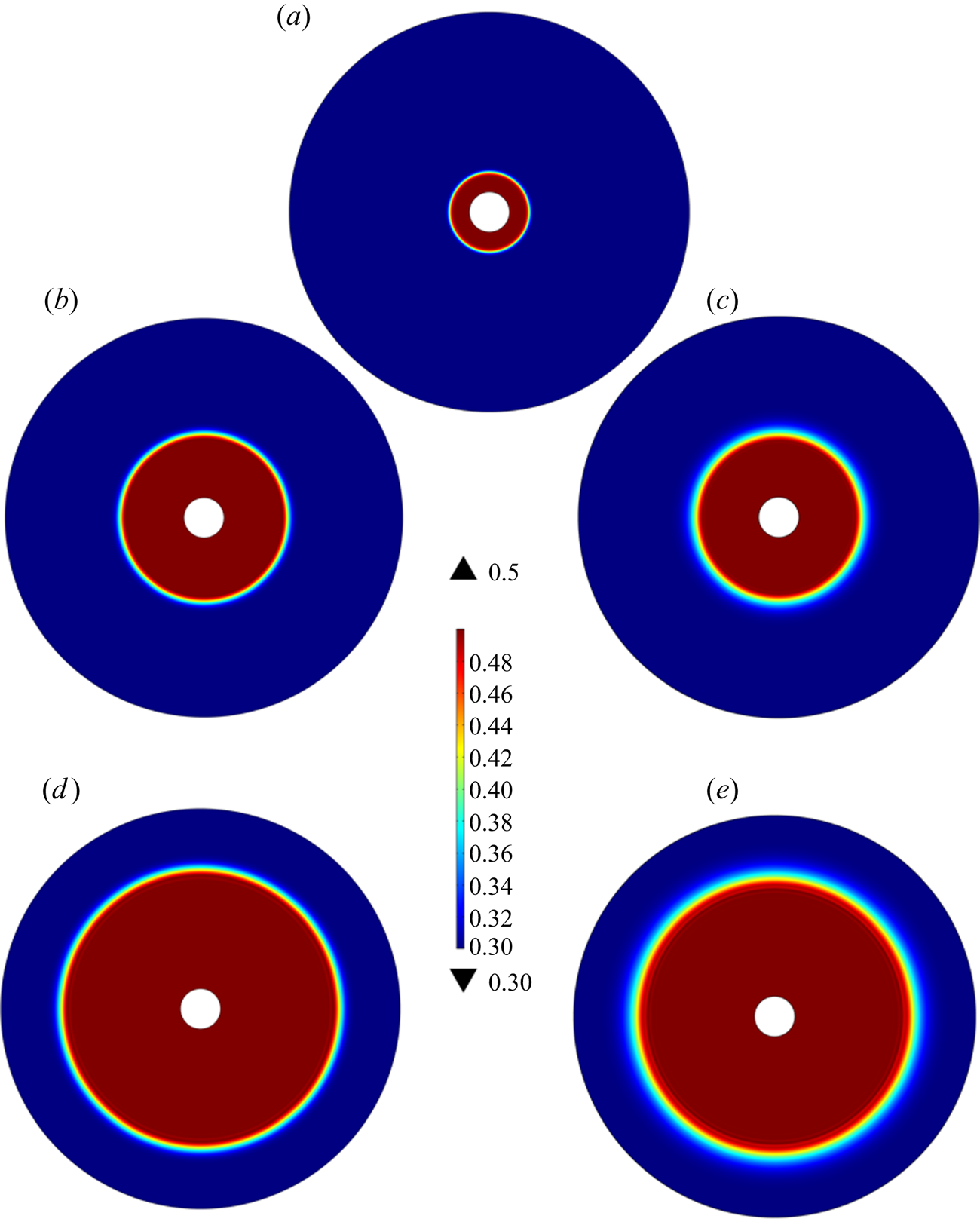
 $(x_1^{\prime },x_2^{\prime })$. To demonstrate this facility, we have shown the results of COMSOL® simulations of a 50 % suspension displacing a 30 % suspension in an expansion geometry and a radial Hele-Shaw geometry in figures 6 and 7, respectively. In the two figures we have also compared the results against the case where
 $\mathcal {D}_{eff}^{\prime }$ is manually set to zero. It may be seen that the inclusion of Taylor dispersion leads to a stronger relaxation of the shock in the flow direction. Third, we note that while the averaging procedure leads to the collapse of one physical dimension, local values of
 $\phi$ and
 $u_i^{\prime }$ may be obtained as a function of
 $x_3^{\prime }$ up to first order in
 $\chi \epsilon$ by substituting
 $\bar {\phi }$,
 $\boldsymbol {\nabla }_{2_i}^{\prime } P^{\prime }$ and
 $\boldsymbol {\nabla }_{2_j}^{\prime }\bar {\phi }\boldsymbol {\nabla }_{2_j}^{\prime } P^{\prime }$ in (3.16), (3.17), (3.33) and (3.35).
Simulation of the displacement of a 30 % suspension by a 50 % suspension in a Hele-Shaw expansion geometry using the macrotransport equations, (4.1) to (4.5), solved on COMSOL®. Subfigure (a) shows the details of the expansion geometry. A pressure difference of  $\Delta P^{\prime }$ is applied between the left and right edges of the geometry. The length, time and velocity scales used to render the equations dimensionless are
 $B^{\prime 3}/a^{\prime 2}$,
 $B^{\prime 4}\mu _0^{\prime }/a^{\prime 4}\Delta P^{\prime }$ and
 $a^{\prime 2}\Delta P^{\prime }/(B^{\prime }\mu _0^{\prime })$. Subfigure (b) shows the initial volume fraction distribution, which contains a shock in the flow direction at
 $x_1=-5$. Subfigures (c–f) show the evolution of the volume fraction distribution predicted by the macrotransport equation, (4.1), at times
 $t=250,750,1500$ and 3000, respectively, for two cases: with Taylor dispersion in (4.1) turned off (top), and with Taylor dispersion turned on (bottom). It can be seen that with the inclusion of Taylor dispersion, the shock relaxes significantly more in the axial direction. The aspect ratio
 $B^{\prime }/a^{\prime }$ for the simulations was 20.

Simulation of the displacement of a 30 % suspension by a 50 % suspension in a radial Hele-Shaw geometry with inner and outer radii of  $1$ and
 $10$ units, respectively. The macrotransport equations, (4.1) to (4.5), were solved in the simulations on COMSOL®. A radial pressure difference of
 $\Delta P^{\prime }$ is applied to drive the suspension flow outwards from the centre. The length, time and velocity scales used to render the equations dimensionless are
 $B^{\prime 3}/a^{\prime 2}$,
 $B^{\prime 4}\mu _0^{\prime }/a^{\prime 4}\Delta P^{\prime }$ and
 $a^{\prime 2}\Delta P^{\prime }/(B^{\prime }\mu _0^{\prime })$. The initial volume fraction distribution,
 $\phi |_{t=0}=0.4+0.1\tanh \left [10(r-2)\right ]$, shows a shock at a radial position,
 $r$, of
 $2$ units (see subfigure a). Subfigures (b,d) show the evolution of volume fraction distribution for
 $t=400$ and
 $t=1600$, respectively, when Taylor dispersion is turned off, while subfigures (c,e) show the results for the case when Taylor dispersion is included for the time stamps
 $t = 400$ and
 $t=1600$, respectively. As in figure 6, the relaxation of the shock in the radial direction is stronger when Taylor dispersion is included in the simulations. The aspect ratio
 $B^{\prime }/a^{\prime }$ for the simulations was 20.

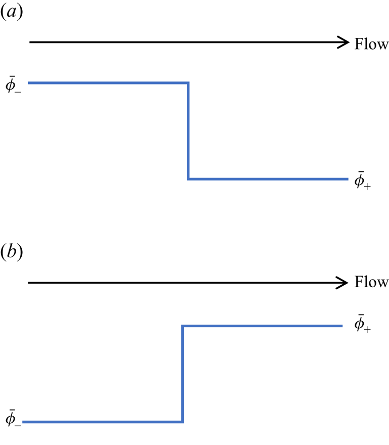
We now investigate the profile evolution with time/strain for two canonical volume fraction distributions in Hele-Shaw geometries: (a) a shock with a negative volume fraction step in the flow direction (see figure 8a), which represents a high volume fraction suspension pushing a low volume fraction suspension ( $\bar {\phi }_->\bar {\phi }_+$), and (b) a shock with a step up in the volume fraction (see figure 8b), which corresponds to a low volume fraction suspension pushing a high volume fraction suspension (
 $\bar {\phi }_-<\bar {\phi }_+$). As discussed in Ramachandran (Reference Ramachandran2013), for the first case, both the convective and the dispersive components of the macrotransport equation act to relax volume fraction gradients and blunt the shock continuously. Let us now consider the more interesting case of a shock with a positive volume fraction gradient along the flow direction. Again, as discussed in the previous work (Ramachandran Reference Ramachandran2013) for flow through a tube, it may be shown that in the frame of reference of the shock velocity,
 $U_{s}$,given by
 \begin{equation} U_s^{\prime }=\left(\frac{g(\phi_{+})-g(\phi_{-})}{\phi_{+}-\phi_{-}}\right)U^{\prime }, \end{equation}
the shock does not decay continuously with increasing strain; instead, the particle distribution reaches a steady state asymptote. The establishment of this solution is the consequence of a balance between the excess of the flow-averaged volume fraction over the area-averaged volume fraction, which causes sharpening of the positive volume fraction gradient, and Taylor dispersion, which acts to relax the gradient. While this mathematical solution exists for the Hele-Shaw geometry, it is physically infeasible. A positive volume fraction shock in the flow direction represents an unfavourable mobility contrast, which is known to render Hele-Shaw flow susceptible to the viscous miscible fingering instability.
Two canonical volume fraction profiles: (a) a step decrease and (b) a step increase in the depth-averaged volume fraction in the flow direction. Here  $\bar {\phi }_-$ and
 $\bar {\phi }_+$ are the volume fractions upstream and downstream of the shock.

Viscous miscible fingering is a classical problem in fluid mechanics (Hill Reference Hill1952; Wooding Reference Wooding1962; Homsy Reference Homsy1987) that was comprehensively analysed for the planar Hele-Shaw geometry in the theoretical works reported by Wooding (Reference Wooding1962), Tan & Homsy (Reference Tan and Homsy1986) and Ben, Demekhin & Chang (Reference Ben, Demekhin and Chang2002). In this paper we closely follow the analysis of Tan & Homsy (Reference Tan and Homsy1986), who considered a step change in the concentration distribution of a solute that impresses an exponential dependence of the solution viscosity on its concentration, for both isotropic and anisotropic instances of the dispersion coefficient. The key result that arises out of their work is the relationship of the rate of growth,  $\sigma ^{\prime }$, of a sinusoidal perturbation to its wavenumber,
 $k^{\prime }$. For long waves,
 $\sigma ^{\prime }\propto k^{\prime }$ and is controlled by the viscosity contrast and the velocity of the flow. For very short waves,
 $\sigma ^{\prime }$ is negative and is proportional to
 $-k^{\prime 2}$, as solute diffusion perpendicular to the flow erases concentration perturbations. Thus, there exists a wavenumber
 $k_{m}^{\prime }$ corresponding to which the growth rate of perturbations reaches a maximum,
 $\sigma _m^{\prime }$.
 $k_{m}^{\prime }$ and
 $\sigma _{m}^{\prime }$ depend on the flow velocity
 $U^{\prime }$, dispersivity along the flow direction
 $(D_\parallel ^{\prime })$ and the diffusivity perpendicular to the flow direction
 $(D_\perp ^{\prime })$. In the limit where the diffusivity normal to the flow becomes weak relative to the dispersion coefficient in the flow direction, i.e. when
 $D_\perp ^{\prime }/D_\parallel ^{\prime }\ll 1$, the growth rate is seen to be controlled to leading order by longitudinal or Taylor dispersion. In this limit,
 $\sigma _m^{\prime }$,
 $k_m^{\prime }$ and the cut-off wavenumber
 $k_c^{\prime }$ (the wavenumber beyond which the growth rates are negative), as predicted by Tan & Homsy (Reference Tan and Homsy1986) are reported in table 1.
The scaling relationships for the maximum growth rate  $(\sigma _{m}^{\prime })$ and the wavenumbers corresponding to the maximum growth rate
 $(k_{m}^{\prime })$ and cut-off
 $(k_{c}^{\prime })$ for the miscible viscous fingering problem, in the limit,
 $D_\perp ^{\prime }/D_\parallel ^{\prime }\ll 1$.

This paper extends this treatment for suspension flow in a Hele-Shaw geometry in § 5.
5. Viscous miscible fingering instability in Hele-Shaw suspension flows
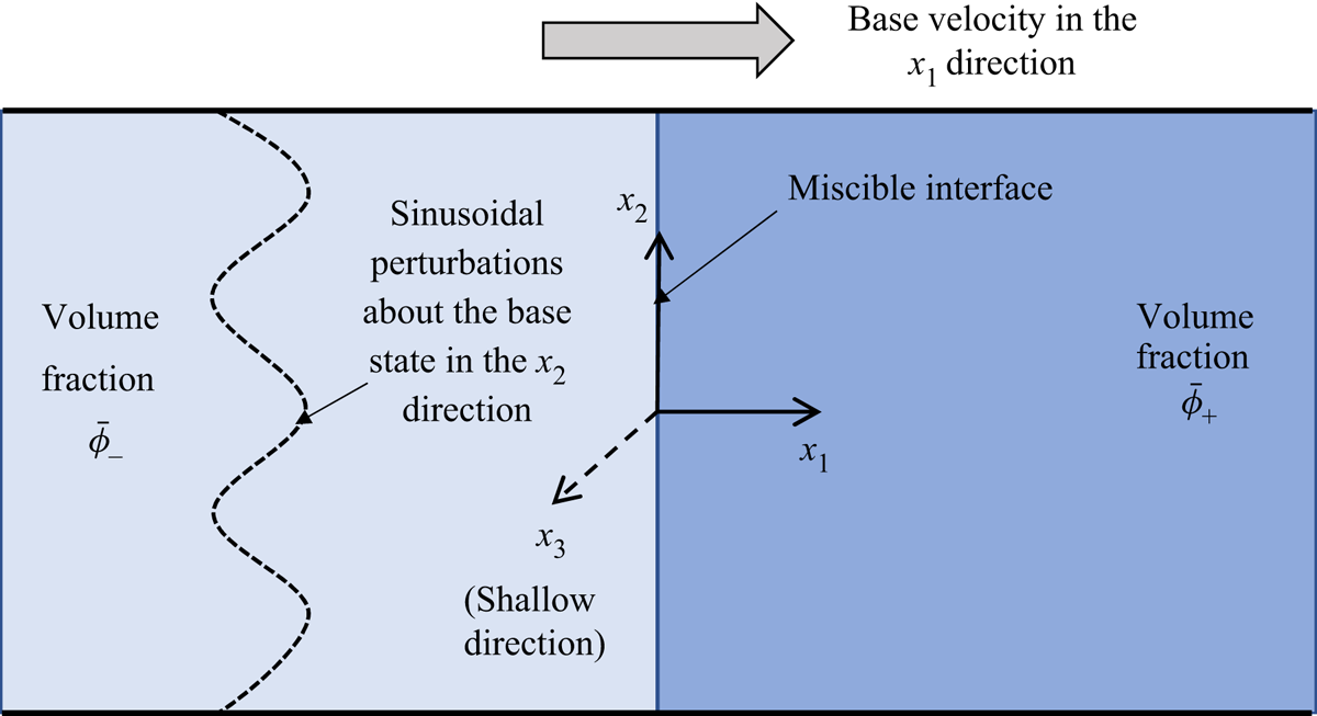
As follows from § 4, we anticipate the case of a low viscosity suspension displacing a high viscosity suspension in a Hele-Shaw geometry to lead to a viscous miscible fingering instability. Here, we analyse the stability of a base state comprising a step increase in the volume fraction across  $x_1=0$ along the flow direction (see schematic in figure 9). Although more sophisticated spectral approaches are possible (Ben et al. Reference Ben, Demekhin and Chang2002), we follow Tan & Homsy (Reference Tan and Homsy1986) by invoking the quasi-steady state approximation (QSSA) to deduce the relationship between the growth rate and wavenumber of a perturbation perpendicular to the flow in the
 $x_2$ direction. The QSSA assumes that the rate of change of the base state is small compared with the rate of growth of the perturbations. Thus, the base state is assumed to be ‘frozen’ in time, and the stability of perturbations about this state is examined. The advantage of this approach is that it permits a semi-analytical solution to the linear stability problem at
 $t=0$. Tan & Homsy (Reference Tan and Homsy1986) provide a comparison of growth rates from QSSA computations against rates from numerical solutions of the governing equations with a random noise as the initial condition. They show that except for a short initial period, there are negligible differences in the results of the growth rates from the two calculations, and that the QSSA treatment captures the essential features of the instability.
Definition sketch for the linear stability analysis of the viscous miscible fingering problem for the Hele-Shaw flow of suspensions. The initial configuration comprises a suspension at a low volume fraction  $\bar {\phi }_-$
 $(x_1<0)$ interfacing a suspension at a high volume fraction
 $\bar {\phi }_+$,
 $x_1>0$, in the form of a flat plane at
 $x_1=0$. The combination is displaced from left to right. Sinusoidal perturbations of the volume fraction, pressure and velocity fields are imposed at about the base configuration in the
 $x_2$ direction.

For the initial volume fraction distribution shown in figure 9, at time  $t=0$, the base state solution profiles for the pressure, volume fraction and velocity obtained from (4.1) to (4.5) and written in the frame of reference of the shock velocity,
 $U_s^{\prime }$ (4.6) are
 $$\begin{gather} \bar{\phi}^{(b)}=\bar{\phi}_-{+}\left(\bar{\phi}_+{-}\bar{\phi}_-\right)\mathcal{H}(x_1^{\prime }), \quad u_1^{\prime (b)}=U^{\prime }-U_s^{\prime }, \quad u_2^{\prime (b)}=0,\nonumber\\ \frac{\partial P^{\prime ^{(b)}}}{\partial x_1^{\prime }}={-}\frac{\mu_0^{\prime }U^{\prime }}{B^{\prime 2}M(\bar{\phi}^{(b)})}. \end{gather}$$
Here, the superscript  $(b)$ denotes the base state, and
 $\mathcal {H}$ is the Heaviside step function. We then introduce normal mode perturbations to the base state volume fraction and pressure distributions,
 \begin{align} \bar{\phi}=\bar{\phi}^{(b)}+\hat{\phi}({\hat{x}_1})\exp\left({({\sigma \hat{t}+\textrm{i}k{\hat{x}_2}})}\right), \quad P^{\prime }=P^{\prime (b)}+\frac{U^{\prime } \mu_{0} \chi}{B}\hat{P}({\hat{x}_1})\exp\left({({\sigma \hat{t}+\textrm{i}k{\hat{x}_2}})}\right). \end{align}
The perturbed equations obtained from (4.1)–(4.5) are rendered dimensionless, using the following scalings:
 \begin{gather}
\sigma =\dfrac{\sigma^{\prime }}{\left(\dfrac{U^{\prime
}}{\chi B}\right)},\quad \hat{t}=\dfrac{t^{\prime
}}{\left(\dfrac{\chi B^{\prime }}{U^{\prime }}\right)},
\quad k=k^{\prime }\chi B^{\prime }, \quad
{\hat{x}_1}=\dfrac{x_1^{\prime }}{\chi B^{\prime }},\notag\\
\hat{P}=\dfrac{P^{\prime
}}{\left(\dfrac{U^{\prime } \mu_{0} \chi}{B^{\prime
}}\right)} \quad \text{with}\ \chi=\dfrac{B^{\prime
2}}{a^{\prime 2}}. \end{gather}
A linearization of the system of equations in (4.1)–(4.5) about the base state followed by the application of QSSA results in the following perturbed forms of the continuity and macro-transport equations:
 \begin{align} &\dfrac{\textrm{d}^{2}\hat{P}}{\textrm{d}{\hat{x}_1}^{2}}-k^{2}\hat{P}=\dfrac{\dfrac{\textrm{d}M}{\textrm{d}\bar{\phi}}(\bar{\phi}^{(b)})}{M^{2}(\bar{\phi}^{(b)})}\dfrac{\textrm{d}\hat{\phi}}{\textrm{d}{\hat{x}_1}}, \end{align}
 \begin{align}
&\left[h(\bar{\phi}^{(b)})+\dfrac{\left(1-b\right)}{\chi^2}q_A(\bar{\phi}^{(b)})\right]
\dfrac{\textrm{d}^2\hat{\phi}}{\textrm{d}\hat{x}_1^2}={-}\dfrac{\left(b+d\right)}{\chi^2}q_B(\bar{\phi}^{(b)})k^2\hat{u}_1\nonumber\\
&\quad +\left\{\dfrac{k^2}{\chi^2}\left[\left(1+d\right)q_A(\bar{\phi}^{(b)})+\left(1+d+\dfrac{(b+d)}{\chi}\right)
q_B(\bar{\phi}^{(b)})\dfrac{\dfrac{\textrm{d}M}{\textrm{d}\bar{\phi}}(\bar{\phi}^{(b)})}{M(\bar{\phi}^{(b)})}\right]+\sigma\right\}\hat{\phi}\nonumber\\
&\quad +\left[\dfrac{\textrm{d}g}{\textrm{d}\bar{\phi}}(\bar{\phi}^{(b)})-\dfrac{U_s^{\prime }}{U^{\prime
}}\right]\dfrac{\textrm{d}\hat{\phi}}{\textrm{d}\hat{x}_1}.
\end{align}
The perturbed velocity  $\hat {u}_1$ appearing in the above equation is given by
 \begin{equation}
\hat{u}_1={-}M(\bar{\phi}^{(b)})\dfrac{\textrm{d}\hat{P}}{\textrm{d}\hat{x}_1}
+\hat{\phi}\dfrac{\dfrac{\textrm{d}M}{\textrm{d}\bar{\phi}}(\bar{\phi}^{(b)})}
{M(\bar{\phi}^{(b)})}.
\end{equation}
The dimensionless ordinary differential equations (ODEs) in (5.4a), (5.4b) and (5.5) represent a system of four first-order ODEs in the variables  $\hat {P}$,
 $\hat {u}_1$,
 $\hat {\phi }$ and
 $\textrm {d}\hat {\phi }/\textrm {d}\hat {x}_1$, and are applicable in each of the two domains,
 $\hat {x}_1<0$ and
 $\hat {x}_1>0$. The ODE system was solved using the eigenvector expansion technique on MATLAB®. The boundary conditions employed were that the perturbed variables vanish as
 $\hat {x}_1\to -\infty$ and
 $\hat {x}_1\to +\infty$, and that
 $\hat {P}$,
 $\hat {u}_1$,
 $\hat {\phi }$ and the total particle flux in the
 $\hat {x}_1$ direction
 $(\hat {J}_1)$, derived separately for
 $\hat {x}_1<0$ and
 $\hat {x}_1>0$, match at
 $\hat {x}_1=0$. The expression for
 $\hat {J}_1$ is
 $$\begin{align}
\hat{J}_1&=\dfrac{\left(1+d\right)}{\chi^2}q_B(\bar{\phi}^{(b)})
M(\bar{\phi}^{(b)})k^2\hat{P}+g(\bar{\phi}^{(b)})\hat{u}_1
+\left[\dfrac{\textrm{d}g}{\textrm{d}\bar{\phi}}(\bar{\phi}^{(b)})-\dfrac{U_s^{\prime
}}{U^{\prime }}\right]\hat{\phi}\nonumber\\
&\quad -\left[h(\bar{\phi}^{(b)})+\dfrac{\left(1-b\right)}{\chi^2}q_A(\bar{\phi}^{(b)})\right]
\dfrac{\textrm{d}\hat{\phi}}{\textrm{d}\hat{x}_1}.
\end{align}$$
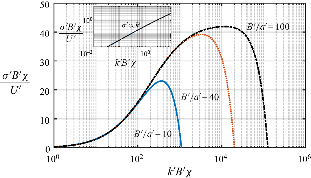
Figure 10 shows the relationship between  $\sigma$ and
 $k$ for
 $B^{\prime }/a^{\prime }=20, 40$ and 100 for the case of
 $\hat {\phi }_-=0.4$ and
 $\hat {\phi }_{+}=0.5$. The behaviour is analogous to the observations of Tan & Homsy (Reference Tan and Homsy1986). For each aspect ratio
 $B/a$,
 $\sigma$ is positive in the long wave limit and increases as
 $k$ (see inset of figure 10). For short waves, however, the perturbations are stabilized by shear-induced migration normal to the flow direction. The dimensionless growth rate corresponding to the fastest growing mode,
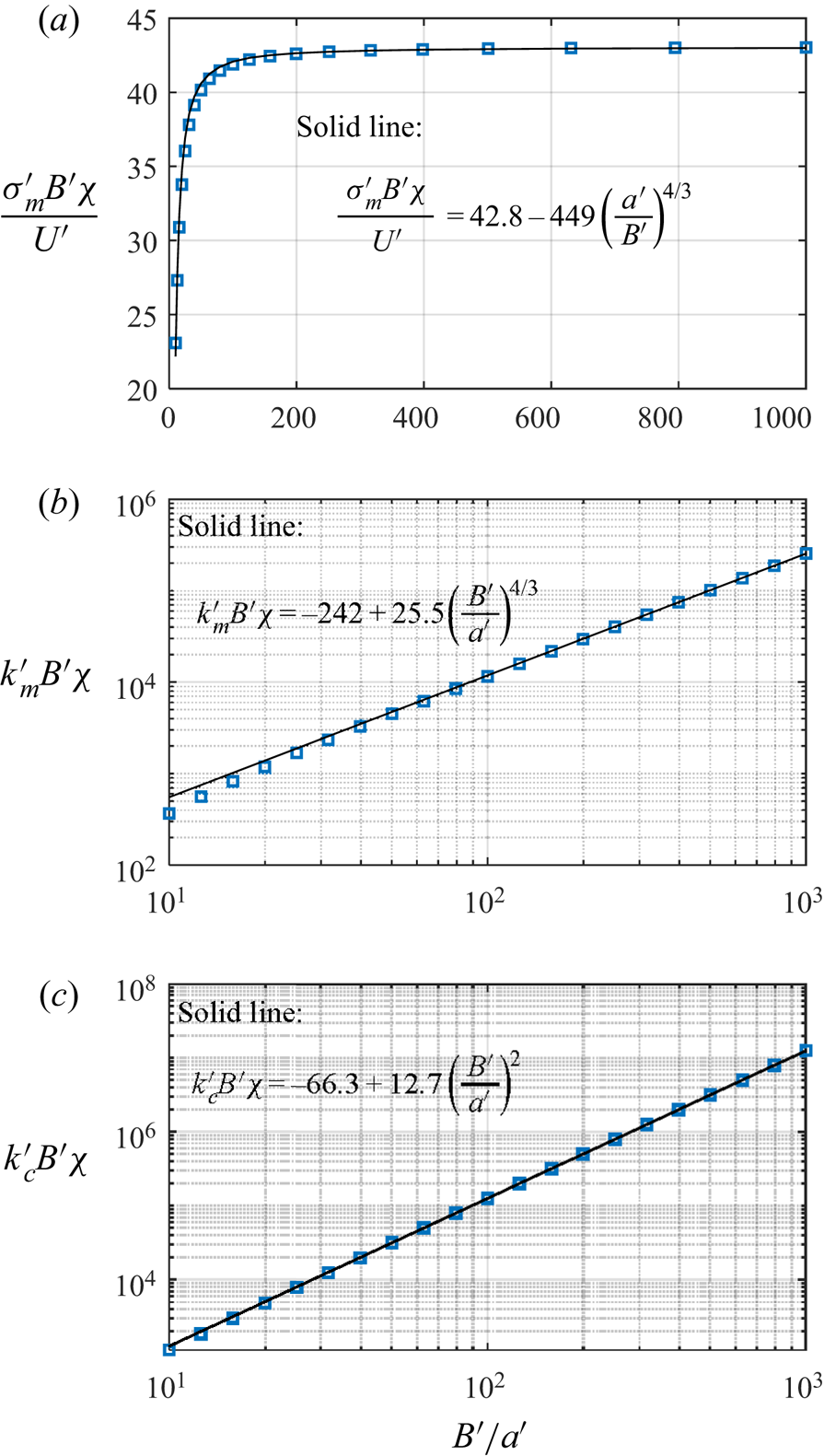
 $\sigma _{m}$, is relatively unaffected by the aspect ratio (see figure 11a). However, the dimensionless wavenumbers
 $k_{m}$ and
 $k_{c}$ corresponding to
 $\sigma _{m}$ and the cut-off (see figure 11b,c), respectively, increase as the aspect ratio increases, i.e. a larger range of high frequency waves falls in the unstable region with an increase in
 $B^{\prime }/a^{\prime }$. This is due to a decrease in the shear-induced migration rate and an increase in the Taylor dispersivity with the increase in the aspect ratio. Figure 11 shows three key variables:
 $\sigma _{m}$,
 $k_{c}$ and
 $k_{m}$, over a range of
 $B^{\prime }/a^{\prime }$ values. We observe that when equivalent parameters are considered for the Hele-Shaw suspension flow problem and the solute problem (Tan & Homsy Reference Tan and Homsy1986), i.e. when the following substitutions are made,
 \begin{equation} D_{{\parallel}}^{\prime
}\sim\frac{U^{\prime }B^{\prime 3}}{a^{\prime 2}},\quad
D_\perp^{\prime}{\sim}\frac{U^{\prime }a^{\prime 2}}{B^{\prime }}
\quad \text{and}\quad \frac{D_\perp^{\prime
}}{D_\parallel^{\prime }} \sim \frac{a^{\prime
4}}{B^{\prime 4}},\end{equation}
the results in figure 11 are in agreement with the theory of Tan & Homsy (Reference Tan and Homsy1986) in the limit  $D_{\perp }^{\prime }/D_{\parallel }^{\prime }\ll 1$ (see table 1), which is valid for the suspension problem as
 $a^{\prime }\ll B^{\prime }$ in most suspension experiments. It follows that
 $k_{m}^{\prime }\propto a^{\prime 2/3}/B^{\prime 5/3}$,
 $k_c^{\prime }\propto {B^{\prime -1}}$ and
 $\sigma _{m}\propto U^{\prime }a^{\prime 2}/B{\prime ^3}$.
The dispersion relationship arising from a linear stability analysis of the macrotransport equation for a step increase in volume fraction in the flow direction from  $\bar {\phi }_-=0.4$ to
 $\bar {\phi }_+=0.5$ (see figure 8b). The solid, dotted and dash–dotted curves are results for
 $B/a =$ 10, 40 and 100, respectively. The inset shows the same dispersion curves in the limit of small wavenumbers.

The maximum growth rate  $\sigma _m^{\prime }$ (subfigure a), the wavenumber,
 $k_m^{\prime }$, corresponding to the maximum growth rate (subfigure b) and the cut-off wavenumber (subfigure c) as functions of the aspect ratio
 $B^{\prime }/a^{\prime }$ for
 $\bar {\phi }_-=0.4$ and
 $\bar {\phi }_+=0.5$.

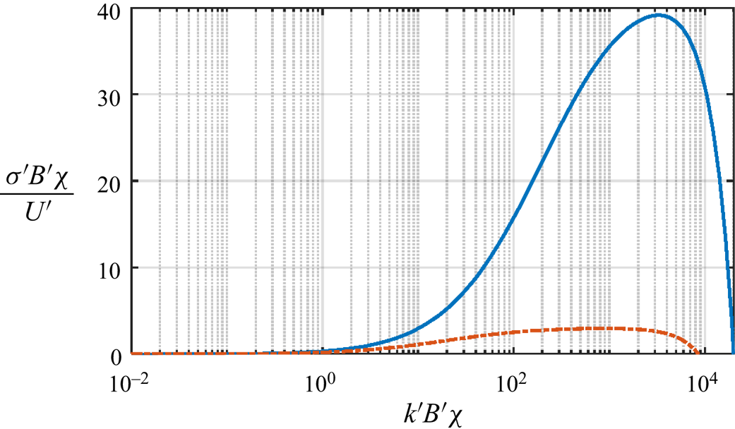
Figure 12 examines the effect of volume fraction on the stability characteristics. It can be seen that for the same step change in volume fraction of 10 %, the growth rates and the range of wavenumbers for which  $\sigma '$ is positive is greatly diminished for
 $\bar {\phi }_-=0.3$ and
 $\bar {\phi }_+=0.4$ as compared with
 $\bar {\phi }_-=0.4$ and
 $\bar {\phi }_+=0.5$. This is primarily due to the highly nonlinear influence of
 $\bar {\phi }$ on the Taylor dispersivity (see figure 4c), and to a lesser extent, on the suspension mobility (see figure 4a) and shear-induced migration rates (see figure 4e,f). It is also instructive to examine the role of the excess of the flow-averaged concentration over the depth-averaged concentration, i.e.
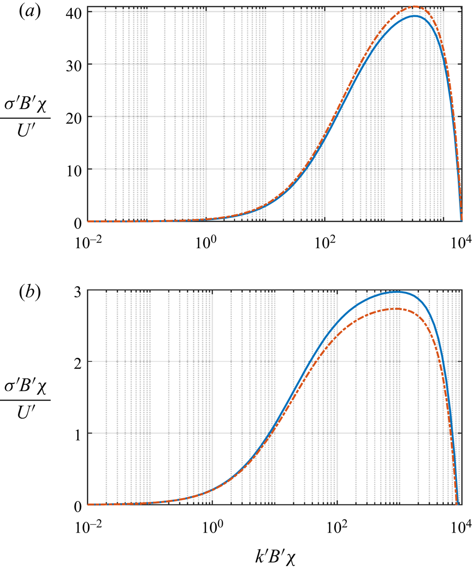
 $g (\bar {\phi })>\bar {\phi }$ on the stability curves, since this is a feature that is different from the work of Wooding (Reference Wooding1962) and Tan & Homsy (Reference Tan and Homsy1986) In figure 13(a) we have shown
 $\sigma '$ vs
 $k'$ for
 $B^{\prime }/a^{\prime }=40$,
 $\bar {\phi }_-=0.4$ and
 $\bar {\phi }_+=0.5$ with
 $g (\bar {\phi })$ set manually to
 $\bar {\phi }$ (dash–dotted curve). As can be seen, in the absence of a difference between
 $g (\bar {\phi })$ and
 $\bar {\phi }$, the growth rates are enhanced at all the shown wavenumbers, with the largest increase occurring near
 $k_m^{\prime }$. On the other hand, for
 $B^{\prime }/a^{\prime }=40$,
 $\bar {\phi }_-=0.3$ and
 $\bar {\phi }_+=0.4$, the opposite effect is observed (see figure 13b); the excess of
 $g (\bar {\phi })$ over
 $\bar {\phi }$ diminishes the growth rates of perturbations. This can be explained as follows. At the higher volume fractions, the shock velocity
 $U_s^{\prime }$ is
 $0.95U'$, i.e. less than
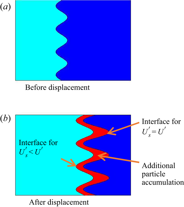
 $U^{\prime }$. This situation is similar to the meniscus accumulation phenomenon (Karnis & Mason Reference Karnis and Mason1967; Chapman Reference Chapman1990; Tang et al. Reference Tang, Grivas, Homentcovschi, Geer and Singler2000; Ramachandran & Leighton Reference Ramachandran and Leighton2007a; Ramachandran Reference Ramachandran2013; Luo, Chen & Lee Reference Luo, Chen and Lee2018), whereby particles accumulate at an advancing interface due to the difference in the particle average velocities behind the meniscus and at the meniscus. The greater the displacement, the thicker the accumulated layer at the shock front. As shown in figure 14, when a perturbed miscible interface is displaced in the flow direction, turning on the physical effect of
 $U_s^{\prime }< U^{\prime }$ would lead to an accumulation of particles at the displaced interface compared with the case when
 $U_s^{\prime }$ is equal to
 $U^{\prime }$. The accumulation manifests as a reduced growth rate of the perturbation. The situation would be exactly the opposite for the case when
 $U_s^{\prime }>U^{\prime }$, which occurs for
 $\bar {\phi }_-=0.3$ and
 $\bar {\phi }_+=0.4$. Consequently, there would be a depletion of particles at the perturbed interface compared with the case of
 $U_s^{\prime }=U^{\prime }$, leading to higher growth rates when
 $g (\bar {\phi })>\bar {\phi }$.
The effect of volume fraction on the stability curve,  $\sigma '$ vs
 $k'$. For the solid curve,
 $\bar {\phi }_-=0.4$ and
 $\bar {\phi }_+=0.5$, while for the dash–dotted curve,
 $\bar {\phi }_-=0.3$ and
 $\bar {\phi }_+=0.4$. For both curves,
 $B^{\prime }/a^{\prime }=40$. Larger volume fractions lead to higher growth rates and a larger range of wavenumbers for which perturbations are unstable.

The effect of the excess of the flow-averaged concentration  $g$ over the area-averaged concentration
 $\bar {\phi }$ on the relationship between
 $\sigma '$ and
 $k'$; (a)
 $\bar {\phi }_-=0.4$ and
 $\bar {\phi }_+=0.5$, (b)
 $\bar {\phi }_-=0.3$ and
 $\bar {\phi }_+=0.4$. For both subfigures,
 $B^{\prime }/a^{\prime }=40$. In each subfigure, the dash–dotted line is the result of a simulation where
 $g$ was manually set to be equal to
 $\bar {\phi }$.

A picture explaining why the case of  $U_s^{\prime }< U^{\prime }$ would lead to lower growth rates compared with the case of
 $U_s^{\prime }=U^{\prime }$. A low volume fraction suspension displaces a high volume fraction suspension from left to right.

We conclude this section with two comments. First, the results above are obtained by invoking the QSSA for a step change in the volume fraction at  $t=0$. At longer times, the base state volume fraction distribution will eventually relax to produce gradients over a length scale of
 $B^{\prime 3}/a^{\prime 2}$. As a consequence, the maximum growth rate and wavenumber will diminish, as observed by Tan & Homsy (Reference Tan and Homsy1986). An investigation of the stability characteristics of the base state solution for
 $t>0$ will be pursued in the future. Second, the critical viscosity predicted from our theory is unity, i.e. the suspension being displaced needs only to be more viscous than the upstream suspension to initiate the instability. However, it has been reported in several recent studies that a critical viscosity contrast less than unity has to be crossed to observe the viscous miscible fingering instability, and this has been attributed to the three-dimensional distribution of the two fluids at the mixing front (Lajeunesse et al. Reference Lajeunesse, Martin, Rakotomalala, Salin and Yortsos1999; Bischofberger, Ramachandran & Nagel Reference Bischofberger, Ramachandran and Nagel2014; Videbaek & Nagel Reference Videbaek and Nagel2019; Luo, Chen & Lee Reference Luo, Chen and Lee2020). Our stability analysis is implemented on a macrotransport equation obtained from an asymptotic expansion, and the inclusion of the Taylor dispersion term does account for the penetration of two fluids in the mixing zone (see the discussion around figure 3). But the observation of a critical viscosity contrast to trigger the instability would imply that we would need to extend the expansion to higher orders to capture the physics. This extension is also left to future work.
6. Conclusions and future work
A depth-averaged macrotransport equation as applicable to concentrated flowing suspensions was derived for the planar Hele-Shaw geometry. The novel contribution of this work is a formal derivation of the expression for Taylor dispersion for Hele-Shaw suspension flows. The Taylor dispersivity scales as  $U_c^{\prime }B^{\prime 3}/a^{\prime 2}$, and is a scaling factor of
 $B^{\prime ^4}/a^{\prime 4}$ larger than the shear-induced migration terms in the macrotransport equation. However, Taylor dispersion produces a particle flux only along the flow direction and, hence, shear-induced migration due to gradients in particle volume fraction, shear rates and streamline curvature is still the dominant mechanism of flux normal to the streamlines. The Taylor dispersion term is expected to enhance the relaxation of negative particle volume fraction gradients along the streamlines. Positive volume fraction gradients along the flow are, however, unstable to viscous miscible fingering. A linear stability analysis with a QSSA was implemented for a step increase in the depth-averaged volume fraction of the suspension in the flow direction. The dispersion relationship for this system qualitatively follows the trends observed by Tan & Homsy (Reference Tan and Homsy1986). In the limit of large aspect ratios
 $(B^{\prime }/a^{\prime }\gg 1)$, the maximum growth rate is controlled by Taylor dispersion, while the ‘most dangerous’ and cut-off wavenumbers are controlled by a combination of Taylor dispersion and shear-induced migration effects (see table 1 for a summary). Future work will focus on the extension of the stability calculations to times where the initial volume fraction profile relaxes and approaches a steady state, and the modelling of the instability in the radial Hele-Shaw flow of suspensions (Luo et al. Reference Luo, Chen and Lee2018) in order to capture the critical viscosity ratio for the instability observed in previous work (Videbaek & Nagel Reference Videbaek and Nagel2019; Luo et al. Reference Luo, Chen and Lee2020)
Direct engineering applications of the macrotransport equation may be considered in rheological techniques (e.g. loading of a Couette rheometer Leighton & Acrivos Reference Leighton and Acrivos1987), radial source flow (Shamu et al. Reference Shamu, Zou, Kotzé, Wiklund and Håkansson2020) or in devices involving the flow of a suspension through a confined geometry such as powder injection molding (Lam et al. Reference Lam, Chen, Tam and Yu2003). Three-dimensional simulations of the particle distribution based on the suspension balance model can be computationally challenging for such geometries as singularities are observed in the regions of weak shear stresses as experienced in previous work (Fang et al. Reference Fang, Mammoli, Brady, Ingber, Mondy and Graham2002; Miller & Morris Reference Miller and Morris2006; Dontsov & Peirce Reference Dontsov and Peirce2014; Dontsov et al. Reference Dontsov, Boronin, Osiptsov and Derbyshev2019). The macrotransport equation derived in this paper reduces the dimensionality of the problem and circumvents the problem of encountering singularities at the centreplane of a Hele-Shaw flow, allowing a relatively quick simulation of the particle, velocity and pressure distributions. Thus, if the lateral length scales in the geometry of interest are much larger than the induction length, we may employ a solution to the macrotransport equation via the use of commercially available solvers to obtain velocity and volume fraction profiles. Hele-Shaw flow of suspensions also occurs during proppant transport (Hormozi & Frigaard Reference Hormozi and Frigaard2017; Dontsov & Peirce Reference Dontsov and Peirce2014; Dontsov et al. Reference Dontsov, Boronin, Osiptsov and Derbyshev2019). Since our model is developed for moderate volume fractions (20–50 %), it is likely unsuitable for simulating the high packing fractions that can occur in proppant flows through fractures. However, past models have included the effects of only convection and shear-induced migration in the macrotransport equation, ignoring Taylor dispersion. We have already demonstrated the importance of Taylor dispersion in the viscous miscible fingering problem for suspension flows and in relaxing shocks along the flow direction. This will motivate improvement of the models in all the above applications to include a Taylor dispersivity, particularly when sharp volume fraction gradients are encountered in the flow direction. In ongoing work, we are investigating the impact of the Taylor dispersion term on the velocity and volume fraction distributions in Hele-Shaw geometries containing turns, bifurcations, expansions, contractions and stagnation points. We are also working on the experimental verification of the predictions of the macrotransport equation for these geometries in microfabricated channels.
Acknowledgements
Dr Ramachandran acknowledges Professor D.T. Leighton Jr. at the University of Notre Dame for discussions during his doctoral work that have inspired this research.
Funding
Dr Ramachandran is grateful to the Canada Research Chair Tier 2 program (File # 950-231-567), the NSERC Discovery Grant #402005 and the Discovery Accelerator Supplement (File #522652522652) that have funded this work.
Declaration of interests
The authors report no conflict of interest.
Author contributions
A.R. derived the macrotransport equation in the paper. S.C. implemented the linear stability analysis of the viscous miscible fingering problem for suspensions and performed the dispersion relationship calculations. S.C. and A.R. wrote the manuscript together.
Appendix A. Glossary of variables used in this paper
Symbols/variables used and their description.

Appendix B. Functions produced in the multiple time scale expansion procedure
 \begin{gather} \phi^{(0)}=\alpha^{{-}1}\left[\frac{\alpha_w}{x_3}\right], \end{gather}
 \begin{gather} F(\bar{\phi},x_3)=\int_{x_3}^1\frac{\xi \,\textrm{d}\xi}{\mu_r\left[\phi^{(0)}(\bar{\phi},\xi)\right]}, \end{gather}
 \begin{gather} M(\bar{\phi})=\int_0^1\frac{\xi^2 \,\textrm{d}\xi}{\mu_r\left[\phi^{(0)}(\bar{\phi},\xi)\right]}, \end{gather}
 \begin{gather} G(\bar{\phi})=\int_0^1F(\bar{\phi},\xi)\phi^{(0)}(\bar{\phi},\xi)\,\textrm{d}\xi, \end{gather}
 \begin{gather} Q_1(\bar{\phi},x_3)=\int_0^{x_3}F(\bar{\phi},\xi)\,\textrm{d}\xi, \end{gather}
 \begin{gather} \hat{Q}_1(\bar{\phi},x_3)=\frac{M^{\prime }(\bar{\phi})}{M^2(\bar{\phi})}Q_1(\bar{\phi},x_3)-\frac{1}{M(\bar{\phi})}\frac{\partial Q_1}{\partial \bar{\phi}}(\bar{\phi},x_3), \end{gather}
 \begin{gather} Q_2(\bar{\phi},x_3)=\int_{x_3}^1\frac{\partial \phi^{(0)}(\bar{\phi},\xi)}{\partial \bar{\phi}}\,\textrm{d}\xi, \end{gather}
 \begin{gather} Q_3(\bar{\phi},x_3)=\int_{x_3}^1F(\bar{\phi},\xi)\phi^{(0)} (\bar{\phi},\xi)\,\textrm{d}\xi, \end{gather}
 \begin{gather} Q_4(\bar{\phi},x_3)=\int_0^{x_3}\frac{9}{2f(\phi^{(0)})}\left[Q_1(\bar{\phi},\xi)\phi^{(0)}(\bar{\phi},\xi)-Q_2(\bar{\phi},\xi)G(\bar{\phi})+Q_3(\bar{\phi},\xi)\right]\,\textrm{d}\xi, \end{gather}
 \begin{gather} Q_5(\bar{\phi},x_3)=\int_0^{x_3}\frac{9}{2f(\phi^{(0)})}\left[\frac{\partial Q_1}{\partial \bar{\phi}}(\bar{\phi},\xi)\phi^{(0)}(\bar{\phi},\xi)-Q_2(\bar{\phi},\xi)G'(\bar{\phi})+\frac{\partial Q_3}{\partial \bar{\phi}}(\bar{\phi},\xi)\right]\,\textrm{d}\xi, \end{gather}
 \begin{gather} Q_6(\bar{\phi},x_3)=Q_5-\frac{M'(\bar{\phi})}{M(\bar{\phi})}Q_4, \end{gather}
 \begin{gather} Q_7(\bar{\phi},x_3)=\dfrac{\alpha(\phi^{(0)})}{\alpha'(\phi^{(0)})\alpha_w}\left[\dfrac{\overline{\left[\dfrac{\alpha(\phi^{(0)})}{\alpha'(\phi^{(0)})}Q_6\right]}}{\overline{\left[\dfrac{\alpha(\phi^{(0)})}{\alpha'(\phi^{(0)})}\right]}}-Q_6\right], \end{gather}
 \begin{gather} Q_8(\bar{\phi},x_3)=\int_{x_3}^1\xi\dfrac{\mu_r'(\phi^{(0)})}{\mu_r^2(\phi^{(0)})}Q_7(\bar{\phi},\xi)\,\textrm{d}\xi, \end{gather}
 \begin{gather} Q_9(\bar{\phi})=\int_0^1Q_8(\bar{\phi},\xi)\,\textrm{d}\xi, \end{gather}
 \begin{gather} Q_{10}(\bar{\phi},x_3)=\dfrac{Q_9(\bar{\phi})}{M(\bar{\phi})}F(\bar{\phi},x_3)-Q_8(\bar{\phi},x_3),\end{gather}
 \begin{gather} Q_{11}(\bar{\phi})={-}\dfrac{1}{M(\bar{\phi})}\int_0^1F(\bar{\phi},\xi)Q_7(\bar{\phi},\xi)\,\textrm{d}\xi, \end{gather}
 \begin{gather} Q_{12}(\bar{\phi})=\dfrac{1}{M(\bar{\phi})}\int_0^1Q_{10}(\bar{\phi},\xi)\phi^{(0)}(\bar{\phi},\xi)\,\textrm{d}\xi, \end{gather}
 \begin{gather} g(\bar{\phi})=\dfrac{G(\bar{\phi})}{M(\bar{\phi})}, \end{gather}
 \begin{gather} h(\bar{\phi})=Q_{11}(\bar{\phi})-Q_{12}(\bar{\phi}). \end{gather}
Appendix C. Determination of the volume fraction perturbation $\phi ^{(1)}$

We begin with (3.21) in the main text of the paper,
 $$\begin{align}
&\frac{\partial \phi^{(0)}}{\partial
\bar{\phi}}\boldsymbol{\nabla}_{2_j}[G(\bar{\phi})\boldsymbol{\nabla}_{2_j}
P^{(0)}]-\boldsymbol{\nabla}_{2_j}(F(\bar{\phi},x_3)\boldsymbol{\nabla}_{2_j}
P^{(0)}\phi^{(0)})\nonumber\\
&\quad +\frac{\partial}{\partial x_3}
(u_3^{(0)}\phi^{(0)})=\frac{2}{9}\,\frac{\partial}{\partial
x_3} \left[f(\phi^{(0)})\frac{\partial
}{\partial x_3} (\alpha\tau )^{(1)}
\right].
\end{align}$$
Integrating (C1) from  $x_3$ to
 $1$, and applying the no-flux boundary condition at the wall (2.12), we get
 $$\begin{align}
&-Q_2(\bar{\phi},x_3)\boldsymbol{\nabla}_{2_j}[G(\bar{\phi})\boldsymbol{\nabla}_{2_j}
P^{(0)}]+\boldsymbol{\nabla}_{2_j}(Q_3(\bar{\phi},\xi)\boldsymbol{\nabla}_{2_j}
P^{(0)})\nonumber\\
&\quad +\boldsymbol{\nabla}_{2_j}[Q_1(\bar{\phi},x_3)\boldsymbol{\nabla}_{2_j}
P^{(0)}]\phi^{(0)}(\bar{\phi},\xi)
=\frac{2}{9}\,f(\phi^{(0)})\frac{\partial
}{\partial x_3}(\alpha\tau )^{(1)},
\end{align}$$
where
 \begin{equation} \left. \begin{gathered} Q_2(\bar{\phi},x_3)=\int_{x_3}^1\frac{\partial \phi^{(0)}(\bar{\phi},\xi)}{\partial \bar{\phi}}\,\textrm{d}\xi,\\ Q_3(\bar{\phi},x_3)=\int_{x_3}^1F(\bar{\phi},\xi)\phi^{(0)}(\bar{\phi},\xi)\,\textrm{d}\xi. \end{gathered} \right\} \end{equation}
Expanding the divergence operations yields
 $$\begin{align}
&(Q_1\phi^{(0)}-Q_2G+Q_3)\boldsymbol{\nabla}_{2}^2P^{(0)}
+\left[\frac{\partial Q_1}{\partial
\bar{\phi}}\phi^{(0)}-Q_2G'(\bar{\phi})+\frac{\partial
Q_3}{\partial
\bar{\phi}}\right]\boldsymbol{\nabla}_{2}\bar{\phi}\boldsymbol{\cdot}\boldsymbol{\nabla}_{2}
P^{(0)}\nonumber\\
&\quad =\frac{2}{9}\,f(\phi^{(0)})\frac{\partial }{\partial
x_3}\left(\alpha\tau \right)^{(1)}.
\end{align}$$
Dividing by  $2f/9$ and integrating from
 $0$ to
 $x_3$,
 \begin{equation} \left(\alpha\tau \right)^{(1)}=Q_4\boldsymbol{\nabla}_{2}^2P^{(0)}+Q_5\boldsymbol{\nabla}_{2}\bar{\phi}\boldsymbol{\cdot}\boldsymbol{\nabla}_{2} P^{(0)}+C_1, \end{equation}
where  $C_1$ is the constant of integration and depends on
 $x_1$ and
 $x_2$ only, and the functions
 $Q_5$ and
 $Q_6$ are defined as
 \begin{equation}
\left. \begin{gathered}
Q_4(\bar{\phi},x_3)=\int_0^{x_3}\frac{9}{2f(\phi^{(0)})}[Q_1(\bar{\phi},\xi)\phi^{(0)}(\bar{\phi},\xi)-Q_2(\bar{\phi},\xi)G(\bar{\phi})+Q_3(\bar{\phi},\xi)]\textrm{d}\xi,
\\
Q_5(\bar{\phi},x_3)=\int_0^{x_3}\frac{9}{2f(\phi^{(0)})}\left[\frac{\partial
Q_1}{\partial
\bar{\phi}}(\bar{\phi},\xi)\phi^{(0)}(\bar{\phi},\xi)-Q_2(\bar{\phi},\xi)G'(\bar{\phi})+\frac{\partial
Q_3}{\partial
\bar{\phi}}(\bar{\phi},\xi)\right]\textrm{d}\xi.
\end{gathered} \right\}
\end{equation}
Using the continuity equation at the zeroth order, we can write
 \begin{equation} M(\bar{\phi})\boldsymbol{\nabla}_{2}^2P^{(0)}+M'(\bar{\phi})\boldsymbol{\nabla}_{2}\bar{\phi}\boldsymbol{\cdot}\boldsymbol{\nabla}_{2} P^{(0)}=0, \end{equation}
and simplify (C5) to
 \begin{equation} \left(\alpha\tau \right)^{(1)}=Q_6\boldsymbol{\nabla}_{2}\bar{\phi}\boldsymbol{\cdot}\boldsymbol{\nabla}_{2} P^{(0)}+C_1, \end{equation}
where
 \begin{equation} Q_6=Q_5-\frac{M'(\bar{\phi})}{M(\bar{\phi})}Q_4. \end{equation}
Now, the particle pressure  $\left (\alpha \tau \right )^{(1)}$ can be expanded as
 \begin{equation} \left(\alpha\tau \right)^{(1)}=\alpha^{(0)}\tau^{(1)}+\alpha^{(1)}\tau^{(0)}. \end{equation}
To obtain  $\tau ^{(1)}$, we perform a perturbation expansion of
 $\tau$ to get
 \begin{equation} \tau^{(1)}=\frac{\boldsymbol{\nabla}_{2_i}P^{(0)}}{\left|\boldsymbol{\nabla}_{2}P^{(0)}\right|}\left(\mu_r\frac{\partial u_i}{\partial x_3}\right)^{(1)}. \end{equation}
The momentum equation at  $O(\epsilon )$ is
 \begin{equation} \frac{\partial}{\partial x_3}\left[\left(\mu_r\frac{\partial u_i}{\partial x_3}\right)^{(1)}\right]=\boldsymbol{\nabla}_{2_j} P^{(1)}. \end{equation}
Integrating (C12) and applying the symmetry condition at the centre, we get
 \begin{equation} \left(\mu_r\frac{\partial u_i}{\partial x_3}\right)^{(1)}=\boldsymbol{\nabla}_{2_i} P^{(1)}x_3. \end{equation}
Therefore,  $\tau ^{(1)}$ becomes
 \begin{equation} \tau^{(1)}=\frac{\boldsymbol{\nabla}_{2}P^{(0)}\boldsymbol{\cdot}\boldsymbol{\nabla}_{2} P^{(1)}}{\left|\boldsymbol{\nabla}_{2}P^{(0)}\right|}x_3. \end{equation}
We can write  $\alpha ^{(1)}$ as
 \begin{equation} \alpha^{(1)}=\alpha'(\phi^{(0)})\phi^{(1)}. \end{equation}
Therefore,
 \begin{equation}
\left(\alpha\tau
\right)^{(1)}=\alpha_w\frac{\boldsymbol{\nabla}_{2}P^{(0)}\boldsymbol{\cdot}\boldsymbol{\nabla}_{2}
P^{(1)}}{|\boldsymbol{\nabla}_{2}P^{(0)}|}+\frac{\alpha'(\phi^{(0)})}{\alpha(\phi^{(0)})}\phi^{(1)}|{
\boldsymbol{\nabla}}_{2}
P^{(0)}|\alpha_w=Q_6\boldsymbol{\nabla}_{2}\bar{\phi}\boldsymbol{\cdot}\boldsymbol{\nabla}_{2}
P^{(0)}+C_1.
\end{equation}
Thus,
 \begin{equation}
\phi^{(1)}
=\frac{\alpha(\phi^{(0)})}{\alpha'(\phi^{(0)})\left|{\boldsymbol{\nabla}}_2
P^{(0)}\right|\alpha_w}
[{-}C(\bar{\phi})+Q_6\boldsymbol{\nabla}_{2}\bar{\phi}\boldsymbol{\cdot}\boldsymbol{\nabla}_{2}
P^{(0)}].
\end{equation}
Since  $\phi ^{(1)}$ is a concentration perturbation, we must have that
 \begin{equation} \overline{\phi^{(1)}}=0, \end{equation}
and, hence,
 \begin{equation} C=\frac{\overline{\left[\dfrac{\alpha(\phi^{(0)})}{\alpha'(\phi^{(0)})}Q_6\right]}} {\overline{\left[\dfrac{\alpha(\phi^{(0)})}{\alpha'(\phi^{(0)})}\right]}}\boldsymbol{\nabla}_{2}\bar{\phi}\boldsymbol{\cdot}\boldsymbol{\nabla}_{2} P^{(0)}. \end{equation}
Thus, the concentration perturbation takes the form
 \begin{equation}
\phi^{(1)}={-}Q_7(\bar{\phi},x_3)\dfrac{\boldsymbol{\nabla}_{2}\bar{\phi}\boldsymbol{\cdot}\boldsymbol{\nabla}_{2}
P^{(0)}}{|{\boldsymbol{\boldsymbol{\nabla}}}_{2}P^{(0)}|},
\end{equation}
where
 \begin{equation} Q_7=\dfrac{\alpha(\phi^{(0)})}{\alpha'(\phi^{(0)})\alpha_w}\left[\dfrac{\overline{\left[\dfrac{\alpha(\phi^{(0)})}{\alpha'(\phi^{(0)})}Q_6\right]}} {\overline{\left[\dfrac{\alpha(\phi^{(0)})}{\alpha'(\phi^{(0)})}\right]}}-Q_6\right]. \end{equation}
This is (3.33) in the main text of the paper.
Appendix D. Determination of the velocity perturbation $u_i^{(1)}$

We first integrate (3.34) in the main text once with respect to  $x_3$, and apply the symmetry condition at the centreline. This yields
 \begin{equation} \left(\mu_r\dfrac{\partial u_i}{\partial x_3}\right)^{(1)}=\boldsymbol{\nabla}_{2_i} P^{(1)}x_3. \end{equation}
Expanding the left-hand side and rearranging we get
 \begin{equation} \mu_r(\phi^{(0)})\frac{\partial u_i^{(1)}}{\partial x_3}=\boldsymbol{\nabla}_{2_i} P^{(1)}x_3-\mu_r'(\phi^{(0)})\phi^{(1)}\frac{\partial u_i^{(0)}}{\partial x_3}. \end{equation}
Using (3.13) that defines the stress at the zeroth order, and (3.33) that defines  $\phi ^{(1)}$, we get
 \begin{equation} \frac{\partial u_i^{(1)}}{\partial x_3}=\frac{x_3}{\mu_r(\phi^{(0)})}\boldsymbol{\nabla}_{2_i} P^{(1)}+\frac{\mu_r'(\phi^{(0)})Q_7x_3}{\mu_r^2(\phi^{(0)})}\frac{\boldsymbol{\nabla}_{2}\bar{\phi}\boldsymbol{\cdot}\boldsymbol{\nabla}_{2}P^{(0)}}{|\boldsymbol{\boldsymbol{\nabla}}_2 P^{(0)}|}\boldsymbol{\nabla}_{2_i} P^{(0)}. \end{equation}
Integrating (D3) with respect to  $x_3$, we obtain
 \begin{equation} u_i^{(1)}={-}F(\bar{\phi},x_3)\boldsymbol{\nabla}_{2_j} P^{(1)}-Q_8(\bar{\phi},x_3)\frac{\boldsymbol{\nabla}_{2}\bar{\phi}\boldsymbol{\cdot}\boldsymbol{\nabla}_{2} P^{(0)}}{{|{\boldsymbol{\nabla}_{2}} P^{(0)}|}}\boldsymbol{\nabla}_{2_i} P^{(0)}, \end{equation}
where
 \begin{equation} Q_8(\bar{\phi},x_3)=\int_{x_3}^1\xi\frac{\mu_r'(\phi^{(0)})}{\mu_r^2(\phi^{(0)})}Q_7(\bar{\phi},\xi)\,\textrm{d}\xi. \end{equation}
Since the depth average of  $u_i^{(1)}$ is zero (see (3.8a,b)),
 \begin{equation} \boldsymbol{\nabla}_{2_i} P^{(1)}={-}\frac{Q_{9}(\bar{\phi})}{M(\bar{\phi})}\frac{\boldsymbol{\nabla}_{2}\bar{\phi}\boldsymbol{\cdot}\boldsymbol{\nabla}_{2} P^{(0)}}{{|{\boldsymbol{\nabla}_{2}} P^{(0)}|}}\boldsymbol{\nabla}_{2_i}P^{(0)}, \end{equation}
where
 \begin{equation} Q_{9}(\bar{\phi})=\int_0^1Q_8(\bar{\phi},\xi)\,\textrm{d}\xi. \end{equation}
Hence,  $u_i^{(1)}$ becomes
 \begin{equation} u_i^{(1)}=Q_{10}(\bar{\phi},x_3)\frac{\boldsymbol{\nabla}_{2}\bar{\phi}\boldsymbol{\cdot}\boldsymbol{\nabla}_{2} P^{(0)}}{{|{\boldsymbol{\nabla}_{2}} P^{(0)}|}}\boldsymbol{\nabla}_{2_i} P^{(0)}, \end{equation}
with
 \begin{equation} Q_{10}(\bar{\phi},x_3)=\frac{Q_9(\bar{\phi})}{M(\bar{\phi})}F(\bar{\phi},x_3)-Q_8(\bar{\phi},x_3). \end{equation}
This is (3.35) in the main text of the paper.